Channel-based algebraic limits to conductive heat transfer

Prashanth S. Venkataram    Sean Molesky Department of Electrical Engineering, Princeton University, Princeton, New Jersey 08544, USA    Juan Carlos Cuevas Departamento de Física Teórica de la Materia Condensada and Condensed Matter Physics Center (IFIMAC), Universidad Autónoma de Madrid, E-28049 Madrid, Spain    Alejandro W. Rodriguez Department of Electrical Engineering, Princeton University, Princeton, New Jersey 08544, USA
(March 18, 2024)
Abstract

Recent experimental advances probing coherent phonon and electron transport in nanoscale devices at contact have motivated theoretical channel-based analyses of conduction based on the nonequilibrium Green’s function formalism. The transmission through each channel has been known to be bounded above by unity, yet actual transmissions in typical systems often fall far below these limits. Building upon recently derived radiative heat transfer limits and a unified formalism characterizing heat transport for arbitrary bosonic systems in the linear regime, we propose new bounds on conductive heat transfer. In particular, we demonstrate that our limits are typically far tighter than the Landauer limits per channel and are close to actual transmission eigenvalues by examining a model of phonon conduction in a 1-dimensional chain. Our limits have ramifications for designing molecular junctions to optimize conduction.

Tailoring nanoscale devices for conductive heat transfer (CHT) is relevant to the design of thermoelectric devices, heat sinks and refrigerators, optoelectronic and optomechanical devices, and for control over chemical reactions at the nanoscale Segal and Agarwalla (2016); Tian et al. (2012, 2014); Bürkle et al. (2015); Klöckner et al. (2017a, b, c); Luo and Chen (2013); Cahill et al. (2014); Pop (2010). Recent experiments have accurately measured thermal conductance through single-atom or molecular junctions Cui et al. (2017); Mosso et al. (2017); Cui et al. (2019); Mosso et al. (2019). Concurrently, phonon and electron conduction have been theoretically described in the linear response regime via the nonequilibrium Green’s function method Cuevas et al. (1998); Segal and Agarwalla (2016); Mingo and Yang (2003); Tian et al. (2012, 2014); Dhar and Roy (2006); Bürkle et al. (2015); Klöckner et al. (2016, 2017a, 2017b, 2017c, 2018); Zhang et al. (2018); Sadasivam et al. (2017); Dubi and Di Ventra (2011). Many of these theoretical works have studied conduction from the perspective of channel-based transmission contributions at each frequency. The transmission from each channel is theoretically bounded above by unity, but in typical systems, the actual transmission falls far short of these limits, and it has been difficult to produce general predictive or explanatory insights regarding which systems may or may not exhibit transmission contributions close to these bounds Klöckner et al. (2017b).

In this paper, building upon an accompanying manuscript Venkataram et al. (2020a), we provide channel-based upper bounds for heat transfer, including CHT, in arbitrary linear bosonic systems that are at least as tight as Landauer limits at each frequency Bürkle et al. (2015); Klöckner et al. (2016, 2017a, 2017b, 2017c, 2018), and in practice are much tighter. First, in Section I, we prove that for the typical system corresponding to a junction connecting two leads, the number of nonzero transmission eigenvalues at each frequency is bounded above by the rank of the response of the junction dressed by the two leads, and this in turn is bounded above by the narrowest bottleneck in the junction. This derivation serves as an algebraic proof or a prior statement based on physical albeit heuristic arguments Cuevas et al. (1998); Bürkle et al. (2015); Klöckner et al. (2016, 2017a, 2017b, 2017c, 2018). Second, in Section II, we show that a recently derived unified framework for heat transfer based on the non-equilibrium Green’s function formalism Venkataram et al. (2020a) can be used to generalize recently proposed bounds on radiative heat transfer (RHT) Molesky et al. (2020); Venkataram et al. (2020b) to include phonon transport; the derivation of these bounds is extremely technical and complex, but we include it in the main text for completeness, and point readers to (16) for the main result. Third, in Section III, we demonstrate the much greater tightness of these bounds for phonon CHT (i.e. coherent thermal phonon transport), relative to the Landauer limits of unity, in a model 1-dimensional chain. Although we do not explicitly consider electron CHT, which is fermionic, the analogous forms of the heat transfer spectrum and analogous properties of the relevant linear response quantities allow for derivation of analogous rank-based and channel-based bounds. Our findings have ramifications for the design of new nanoscale junctions for efficient CHT.

I Rank-based bounds

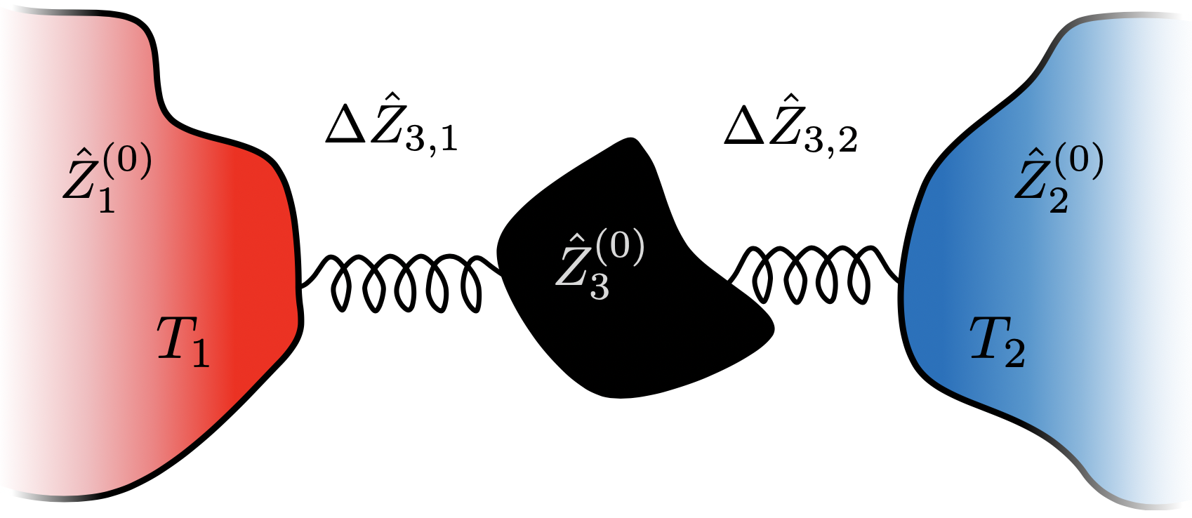
We consider the system depicted schematically in Fig. 1, consisting of two arbitrary components, labeled 1 and 2, exchanging energy only via couplings to a third body 3. Physical embodiments include RHT between any two bodies, as well as CHT for two bodies connected only through a junction Venkataram et al. (2020a). If each component exhibits linear bosonic response with linear couplings, the net heat transfer power may be written as

$$P_{1\to 2}=\int_{0}^{\infty}[\Pi(\omega,T_{2})-\Pi(\omega,T_{1})]\Phi(\omega)\leavevmode\nobreak\ \frac{\mathrm{d}\omega}{2\pi}$$ (1)

where $\Pi(\omega,T)=\hbar\omega/(e^{\hbar\omega/(k_{\mathrm{B}}T)}-1)$ is the Planck function, while $\Phi(\omega)$ is the dimensionless spectrum of energy transfer. The frequency domain equations of motion defining the response of each component $n\in\{1,2,3\}$ in isolation are given through the linear operators $\hat{Z}^{(0)}_{n}$ and their inverses $\hat{Y}^{(0)}_{n}=\hat{Z}^{(0)-1}_{n}$, and the linear coupling of each component $n\in\{1,2\}$ to component 3 is $\Delta\hat{Z}_{3,n}$. Reciprocity means that at any frequency $\omega$, $\hat{Z}^{(0)}_{n}=(\hat{Z}^{(0)}_{n})^{\top}$ must hold, though that may be complex-valued, but we assume $\Delta\hat{Z}_{3,n}=(\Delta\hat{Z}_{n,3})^{\top}$ to be real-valued. Furthermore, passivity means that $\operatorname{asym}(\hat{Y}^{(0)}_{n})=\operatorname{Im}(\hat{Y}^{(0)}_{n})$ for $n\in\{1,2,3\}$ are all positive-semidefinite operators. Throughout this paper, we assume that if the coupling induces an effective nonzero $\Delta\hat{Z}_{nn}$ for each $n\in\{1,2,3\}$, that is included in the definition of $\hat{Z}^{(0)}_{n}$. As examples, the relevant material response functions $\hat{Z}^{(0)}_{n}$ for RHT will generally include the effects of short-range Coulomb interactions, and the electromagnetic couplings (charges) $\Delta\hat{Z}_{n,3}$ will only be for explicitly long-range interactions; for phonon CHT, the specific example of two 1D harmonic oscillators $n\in\{1,2\}$ of masses $m_{n}$ coupled to each other with strength $k_{1,2}$ and each to a separate fixed wall with strength $k_{nn}$ has equations of motion $(k_{1,1}+k_{1,2}-\omega^{2}m_{1})x_{1}-k_{1,2}x_{2}=F_{1}$ and $-k_{1,2}x_{1}+(k_{2,2}+k_{1,2}-\omega^{2}m_{2})x_{2}=F_{2}$, so $\hat{Z}^{(0)}_{n}=k_{nn}+k_{1,2}-\omega^{2}m_{n}$. Finally, throughout this paper, we assume that no degrees of freedom (DOFs) in component 3 are simultaneously coupled to components 1 and 2, which is true of RHT when the material bodies do not overlap, and can be assumed of CHT by expanding the definition of the central junction to prohibit such overlaps; we do this for conceptual and computational simplicity, though the formula for heat transfer and our bounds can be generalized to incorporate other scenarios. Given this, we may write the energy transfer spectrum at each $\omega$ as Venkataram et al. (2020a)

$$\Phi=4\leavevmode\nobreak\ {\rm Tr}\left[\operatorname{asym}(\Delta\hat{Z}_{3,1}\hat{Y}^{(0)}_{1}\Delta\hat{Z}_{1,3})\hat{Y}_{3}^{\dagger}\right.\times\\ \left.\operatorname{asym}(\Delta\hat{Z}_{3,2}\hat{Y}^{(0)}_{2}\Delta\hat{Z}_{2,3})\hat{Y}_{3}\right],$$ (2)

where we define $\hat{Y}_{3}=(\hat{Z}^{(0)}_{3}-\Delta\hat{Z}_{3,1}\hat{Y}^{(0)}_{1}\Delta\hat{Z}_{1,3}-\Delta\hat{Z}_{3,2}\hat{Y}^{(0)}_{2}\Delta\hat{Z}_{2,3})^{-1}$ as the response of component 3 dressed by its couplings to components 1 and 2. For clarity, Appendix B gives correspondences between these abstract operators and concrete linear response quantities in the context of phonon CHT; as examples, in the context of phonon CHT between two leads across a junction, $\hat{Y}_{3}$ is the Green’s function of the junction dressed by the leads, and the operators $\Delta\hat{Z}_{3,n}\operatorname{asym}(\hat{Y}^{(0)}_{n})\Delta\hat{Z}_{n,3}$ for $n\in\{1,2\}$ are the imaginary parts of the self-energies of the leads.

Refer to caption
Figure 1: Schematic system. Two components, labeled 1 & 2, with linear response functions $\hat{Z}^{(0)}_{1}$ and $\hat{Z}^{(0)}_{2}$ and maintained at temperatures $T_{1}$ and $T_{2}$, exchange energy by virtue of coupling to a third component, labeled 3 with linear response function $\hat{Z}^{(0)}_{3}$, through couplings $\Delta\hat{Z}_{3,1}$ and $\Delta\hat{Z}_{3,2}$. All relevant response quantities are assumed to be linear, reciprocal, causal, and passive.

In the context of CHT, components 1 and 2 frequently correspond to large leads, while component 3 corresponds to a much smaller intermediate junction Bürkle et al. (2015); Klöckner et al. (2016, 2017a, 2017b, 2017c, 2018). As the operators in the trace in (2) can be cyclically rearranged, $\Phi$ can be written as the trace of a Hermitian positive-semidefinite operator, and it has already been shown Venkataram et al. (2020a) that its eigenvalues, representing transmission values associated with individual conduction channels, all lie in the range $[0,1]$. Going further, we note that the transmission eigenvalues are the squares of the singular values of the operator $\operatorname{asym}(\Delta\hat{Z}_{3,2}\hat{Y}^{(0)}_{2}\Delta\hat{Z}_{2,3})^{1/2}\hat{Y}_{3}\operatorname{asym}(\Delta\hat{Z}_{3,1}\hat{Y}^{(0)}_{1}\Delta\hat{Z}_{1,3})^{1/2}$, lying in the same range. The number of nonzero singular values is the rank of this operator, which is bounded above by the rank of the various operators being multiplied together, namely $\operatorname{asym}(\Delta\hat{Z}_{3,n}\hat{Y}^{(0)}_{n}\Delta\hat{Z}_{n,3})^{1/2}$ for $n\in\{1,2\}$, along with $\hat{P}_{3(2)}\hat{Y}_{3}\hat{P}_{3(1)}$, where $\hat{P}_{3(n)}=(\hat{P}_{3(n)})^{\top}$ is the orthogonal projection into the subspace of component 3 coupled to component $n\in\{1,2\}$. Therefore, the number of nonzero transmission eigenvalues is bounded above by the minimum of the number of DOFs of component 3 coupled to component 1 versus 2, or the number of DOFs of components 1 or 2 coupled to component 3 (in case the couplings are not one-to-one per DOF in each component). However, even tighter bounds on the number of nonzero transmission eigenvalues can be derived with the following observation. Frequently, component 3 has a narrow bottleneck that has even fewer DOFs than those coupling to components 1 or 2, and if that bottleneck is not directly coupled to components 1 or 2, then component 3 can be divided into subparts A, B, and C, such that subparts A and B couple directly respectively to components 1 and 2 and also to subpart C, while subpart C only couples directly to subparts A and B. This means that $\hat{P}_{3(1)}=\hat{P}_{3\mathrm{A}(1)}$ and $\hat{P}_{3(2)}=\hat{P}_{3\mathrm{B}(2)}$, while we define the nonzero blocks of $\Delta\hat{Z}_{1,3}$ and $\Delta\hat{Z}_{2,3}$ as $\Delta\hat{Z}_{1,3\mathrm{A}}$ and $\Delta\hat{Z}_{2,3\mathrm{B}}$ respectively. Writing the operators in the space of component 3 in block form in terms of the subparts, so that $\hat{Y}_{3}^{-1}$ is given by

$$\hat{Z}^{(0)}_{3}-\Delta\hat{Z}_{3,1}\hat{Y}^{(0)}_{1}\Delta\hat{Z}_{1,3}-\Delta\hat{Z}_{3,2}\hat{Y}^{(0)}_{2}\Delta\hat{Z}_{2,3}=\begin{bmatrix}\hat{Z}^{(0)}_{3\mathrm{A}}-\Delta\hat{Z}_{3\mathrm{A},1}\hat{Y}^{(0)}_{1}\Delta\hat{Z}_{1,3\mathrm{A}}&0&\Delta\hat{Z}_{3\mathrm{AC}}\\ 0&\hat{Z}^{(0)}_{3\mathrm{B}}-\Delta\hat{Z}_{3\mathrm{B},2}\hat{Y}^{(0)}_{2}\Delta\hat{Z}_{2,3\mathrm{B}}&\Delta\hat{Z}_{3\mathrm{BC}}\\ \Delta\hat{Z}_{3\mathrm{CA}}&\Delta\hat{Z}_{3\mathrm{CB}}&\hat{Z}^{(0)}_{3\mathrm{C}}\end{bmatrix}$$

then we may perform the inversion blockwise to yield the B-A off-diagonal subpart block, which is the only relevant nonzero block for energy exchange in this scenario, as $\hat{P}_{3(2)}\hat{Y}_{3}\hat{P}_{3(1)}=\hat{P}_{3\mathrm{B}(2)}(\hat{Z}^{(0)}_{3\mathrm{B}}-\Delta\hat{Z}_{3\mathrm{B},2}\hat{Y}^{(0)}_{2}\Delta\hat{Z}_{2,3\mathrm{B}})^{-1}\Delta\hat{Z}_{3\mathrm{BC}}(\hat{Z}^{(0)}_{3\mathrm{C}}-\Delta\hat{Z}_{3\mathrm{CA}}(\hat{Z}^{(0)}_{3\mathrm{A}}-\Delta\hat{Z}_{3\mathrm{A},1}\hat{Y}^{(0)}_{1}\Delta\hat{Z}_{1,3\mathrm{A}})^{-1}\Delta\hat{Z}_{3\mathrm{AC}}-\Delta\hat{Z}_{3\mathrm{CB}}(\hat{Z}^{(0)}_{3\mathrm{B}}-\Delta\hat{Z}_{3\mathrm{B},2}\hat{Y}^{(0)}_{2}\Delta\hat{Z}_{2,3\mathrm{B}})^{-1}\Delta\hat{Z}_{3\mathrm{BC}})^{-1}\Delta\hat{Z}_{3\mathrm{CA}}(\hat{Z}^{(0)}_{3\mathrm{A}}-\Delta\hat{Z}_{3\mathrm{A},1}\hat{Y}^{(0)}_{1}\Delta\hat{Z}_{1,3\mathrm{A}})^{-1}\hat{P}_{3\mathrm{A}(1)}$. In this expression, the middle operator is nonzero only in the space of subpart C, so if subpart C has the fewest DOFs, then it is the rank-limiting part. It follows that the number of nonzero transmission eigenvalues for two leads exchanging energy via a junction is bounded above by the number of DOFs in the smallest bottleneck in the junction, validating prior observations Cuevas et al. (1998); Bürkle et al. (2015); Klöckner et al. (2016, 2017a, 2017b, 2017c, 2018).

II Channel-based bounds

In order to derive upper bounds on $\Phi$ (no longer assuming any particular division of component 3 into subparts) from (2), we rewrite $\Phi$ as follows. First, we recognize that reciprocity of the relevant operators allows replacement of the Hermitian adjoint by the complex conjugate , and in turn of $\operatorname{asym}$ by $\operatorname{Im}$. Second, we assume that for each of the end components ($n\in\{1,2\}$) connected to the middle component ($3$), the operator $\Delta\hat{Z}_{3,n}\hat{Y}^{(0)}_{n}\Delta\hat{Z}_{n,3}$ for a given $n$ is invertible within the space of DOFs of component 3 which are coupled to that component $n$. This allows for rewriting

$$\operatorname{Im}(\Delta\hat{Z}_{3,n}\hat{Y}^{(0)}_{n}\Delta\hat{Z}_{n,3})=\Delta\hat{Z}_{3,n}\hat{Y}^{(0)\star}_{n}\Delta\hat{Z}_{n,3}\times\\ \operatorname{Im}((\Delta\hat{Z}_{3,n}\hat{Y}^{(0)\star}_{n}\Delta\hat{Z}_{n,3})^{-1})\Delta\hat{Z}_{3,n}\hat{Y}^{(0)}_{n}\Delta\hat{Z}_{n,3}.$$

For notational convenience, in analogy with electromagnetic notation, we denote $\hat{V}_{n}\equiv\Delta\hat{Z}_{3,n}\hat{Y}^{(0)}_{n}\Delta\hat{Z}_{n,3}$; this denotes the response of component $n\in\{1,2\}$ evaluated in the space of DOFs of component 3 coupled to component $n$ (multiplied by those coupling quantities), and in the context of CHT, these are the self-energies of the leads $n$ coupled to the junction (component 3). This therefore allows for writing

$$\Phi=4\leavevmode\nobreak\ {\rm Tr}\left[\hat{V}_{1}\operatorname{Im}(\hat{V}_{1}^{-1\star})\hat{V}_{1}^{\star}\hat{Y}_{3}^{\star}\hat{V}_{2}^{\star}\operatorname{Im}(\hat{V}_{2}^{-1\star})\hat{V}_{2}\hat{Y}_{3}\right]$$

after rearranging the trace. It is also helpful at this point to use the definition $\hat{Y}_{3}=(\hat{Z}^{(0)}_{3}-\hat{V}_{1}-\hat{V}_{2})^{-1}$ to show that $\hat{V}_{2}\hat{Y}_{3}\hat{V}_{1}=\hat{V}_{2}(\hat{1}-(\hat{1}-\hat{Y}^{(0)}_{3}\hat{V}_{1})^{-1}\hat{Y}^{(0)}_{3}\hat{V}_{2})^{-1}\hat{Y}^{(0)}_{3}\hat{V}_{1}(\hat{1}-\hat{Y}^{(0)}_{3}\hat{V}_{1})^{-1}$, as this will become useful for the derivations of these bounds.

Having established these operator definitions and relations, our derivation proceeds following the derivation of the RHT bounds in Molesky et al. (2020). First, we establish and explain generalizations of constraints on quantities like “far-field scattering” relevant to RHT. Second, we apply a lemma by von Neumann Mirsky (1975) (whose derivation is reproduced in context in Molesky et al. (2020)), showing that the largest real positive value of the trace of a product of operators arises when those operators share singular vectors and when the sets of fixed singular values are arranged in consistent orders, to the maximization of $\Phi$, explaining along the way how variation of the singular values themselves is consistent with the conditions of the lemma. We conclude the section by restating the bound for $\Phi$, which we term $\Phi_{\mathrm{opt}}$, and by discussing its implications.

II.1 Constraints on nonnegative far-field scattering

In Venkataram et al. (2020a), we established that in the context of RHT, component 3 corresponds to the vacuum electromagnetic field, so $\hat{Y}^{(0)}_{3}$ would be the vacuum Maxwell Green’s function. We extend this analogy in the other direction to derive constraints on the linear response quantities relevant to this system of two components coupled only via a third.

First, we define the relevant general equations of motion for these operators in order to properly define what is meant by absorbed, scattered, and extinguished power. In Venkataram et al. (2020a), we generally showed that they can be written as $|x\rangle=|x^{(0)}\rangle+\hat{Y}^{(0)}|F\rangle$ along with $|F\rangle=-\Delta\hat{Z}|x\rangle$ where there are nonzero generalized free displacements but no generalized external forces. Here, we do the opposite in order to describe powers in response to generalized forces, so the relevant equations of motion are $|x\rangle=\hat{Y}^{(0)}|F\rangle$ and $|F\rangle=|F^{(0)}\rangle-\Delta\hat{Z}|x\rangle$; for this particular derivation, these are effectively related by the replacement $|F^{(0)}\rangle\leftrightarrow\hat{Z}^{(0)}|x\rangle$. For this system of two components labeled 1 & 2 connected via a third labeled 3, these quantities may be defined in block form as

$$|x\rangle=\begin{bmatrix}|x_{1}\rangle\\ |x_{2}\rangle\\ |x_{3}\rangle\end{bmatrix},\leavevmode\nobreak\ |F\rangle=\begin{bmatrix}|F_{1}\rangle\\ |F_{2}\rangle\\ |F_{3}\rangle\end{bmatrix},\leavevmode\nobreak\ |F^{(0)}\rangle=\begin{bmatrix}|F^{(0)}_{1}\rangle\\ |F^{(0)}_{2}\rangle\\ |F^{(0)}_{3}\rangle\end{bmatrix}\\ \hat{Z}^{(0)}=\begin{bmatrix}\hat{Z}^{(0)}_{1}&0&0\\ 0&\hat{Z}^{(0)}_{2}&0\\ 0&0&\hat{Z}^{(0)}_{3}\end{bmatrix},\leavevmode\nobreak\ \Delta\hat{Z}=\begin{bmatrix}0&0&\Delta\hat{Z}_{1,3}\\ 0&0&\Delta\hat{Z}_{2,3}\\ \Delta\hat{Z}_{3,1}&\Delta\hat{Z}_{3,2}&0\end{bmatrix}$$ (3)

and for further convenience, we define the sub-groups,

$$|x_{\mathrm{A}}\rangle=\begin{bmatrix}|x_{1}\rangle\\ |x_{2}\rangle\end{bmatrix},\leavevmode\nobreak\ |F_{\mathrm{A}}\rangle=\begin{bmatrix}|F_{1}\rangle\\ |F_{2}\rangle\end{bmatrix},\leavevmode\nobreak\ |F^{(0)}_{\mathrm{A}}\rangle=\begin{bmatrix}|F^{(0)}_{1}\rangle\\ |F^{(0)}_{2}\rangle\end{bmatrix}\\ \hat{Z}^{(0)}_{\mathrm{A}}=\begin{bmatrix}\hat{Z}^{(0)}_{1}&0\\ 0&\hat{Z}^{(0)}_{2}\end{bmatrix},\leavevmode\nobreak\ \Delta\hat{Z}_{\mathrm{A},3}=\begin{bmatrix}\Delta\hat{Z}_{1,3}\\ \Delta\hat{Z}_{2,3}\end{bmatrix}$$ (4)

where the subscript “A” refers to the “aggregate” of the components 1 & 2 that are not directly coupled to each other (and $\Delta\hat{Z}_{3,\mathrm{A}}=(\Delta\hat{Z}_{\mathrm{A},3})^{\top}$).

Next, we define the notions of absorbed, scattered, and extinguished power in this system. For RHT, it is simple to see that far-field scattering involves the transfer of energy to component 3, namely the vacuum electromagnetic field, while absorption involves the transfer of energy to components 1 or 2 Miller et al. (2016). We generalize this as follows. We assume that all external forces are only in components 1 or 2, so $|F^{(0)}_{3}\rangle=0$, but $|F^{(0)}_{\mathrm{A}}\rangle\neq 0$. We also define the orthogonal projection operators $\hat{P}_{n}$ which project onto the subspaces of DOFs of component $n\in\{1,2,3\}$; these are orthogonal to each other, so we also define the “aggregate” projection $\hat{P}_{\mathrm{A}}=\hat{P}_{1}+\hat{P}_{2}$. Similarly, we define the “aggregate” response operator $\hat{V}_{\mathrm{A}}=\hat{V}_{1}+\hat{V}_{2}=\Delta\hat{Z}_{3,\mathrm{A}}\hat{Y}^{(0)}_{\mathrm{A}}\Delta\hat{Z}_{\mathrm{A},3}$, but we do not yet assume that the DOFs of component 3 that couple to each of the other components exist in orthogonal subspaces. From these definitions, one finds that absorbed power $\Phi_{\mathrm{abs}}=\frac{\omega}{2}\operatorname{Im}(\langle F,\hat{P}_{\mathrm{A}}x\rangle)$ refers to the energy dumped by the external forces into components 1 & 2, extinguished power $\Phi_{\mathrm{ext}}=\frac{\omega}{2}\operatorname{Im}(\langle F^{(0)},\hat{P}_{\mathrm{A}}x\rangle)$ is the energy dumped by the external forces into the entire system, and scattered power $\Phi_{\mathrm{sca}}=\Phi_{\mathrm{ext}}-\Phi_{\mathrm{abs}}$ is simply the difference of the two.

At this point, we may now generally compute these power quantities for a general external force $|F^{(0)}_{\mathrm{A}}\rangle$. The equations of motion may be written as

$$\begin{split}\hat{Z}^{(0)}_{\mathrm{A}}|x_{\mathrm{A}}\rangle+\Delta\hat{Z}_{\mathrm{A},3}|x_{3}\rangle&=|F^{(0)}_{\mathrm{A}}\rangle\\ \Delta\hat{Z}_{3,\mathrm{A}}|x_{\mathrm{A}}\rangle+\hat{Z}^{(0)}_{3}|x_{3}\rangle&=0\end{split}$$ (5)

whose formal solution may be written as

$$\begin{split}|x_{\mathrm{A}}\rangle&=\hat{Y}^{(0)}_{\mathrm{A}}(\hat{1}+\Delta\hat{Z}_{\mathrm{A},3}\hat{Y}^{(0)}_{3}(\hat{1}-\hat{V}_{\mathrm{A}}\hat{Y}^{(0)}_{3})^{-1}\Delta\hat{Z}_{3,\mathrm{A}}\hat{Y}^{(0)}_{\mathrm{A}})|F^{(0)}_{\mathrm{A}}\rangle\\ |x_{3}\rangle&=-\hat{Y}^{(0)}_{3}(\hat{1}-\hat{V}_{\mathrm{A}}\hat{Y}^{(0)}_{3})^{-1}\Delta\hat{Z}_{3,\mathrm{A}}\hat{Y}^{(0)}_{\mathrm{A}}|F^{(0)}_{\mathrm{A}}\rangle\end{split}$$ (6)

in terms of $|F^{(0)}_{\mathrm{A}}\rangle$. From this, we write the absorbed power $\Phi_{\mathrm{abs}}=\frac{\omega}{2}\operatorname{Im}(\langle F,\hat{P}_{\mathrm{A}}x\rangle)$ (after relevant operator manipulations) as

$$\frac{2}{\omega}\Phi_{\mathrm{abs}}=\langle F^{(0)}_{\mathrm{A}},\hat{Y}^{(0)\star}_{\mathrm{A}}\Delta\hat{Z}_{\mathrm{A},3}(\hat{1}-\hat{Y}^{(0)\star}_{3}\hat{V}_{\mathrm{A}}^{\star})^{-1}\hat{Y}^{(0)\star}_{3}\times\\ \operatorname{Im}(\hat{V}_{\mathrm{A}})\hat{Y}^{(0)}_{3}(\hat{1}-\hat{V}_{\mathrm{A}}\hat{Y}^{(0)}_{3})^{-1}\Delta\hat{Z}_{3,\mathrm{A}}\hat{Y}^{(0)}_{\mathrm{A}}F^{(0)}_{\mathrm{A}}\rangle$$ (7)

upon using the real-valued nature of $\Delta\hat{Z}_{\mathrm{A},3}$ and its transpose, and the fact that for operators $\hat{A}$ and $\hat{B}$, $\operatorname{asym}(\hat{A}^{\dagger}\hat{B}\hat{A})=\hat{A}^{\dagger}\operatorname{asym}(\hat{B})\hat{A}$ (with a similar statement holding for reciprocal operators with the complex conjugate and the imaginary part); passivity means that $\operatorname{Im}(\hat{V}_{n})$ is positive-semidefinite for $n\in\{1,2\}$, and so is $\operatorname{Im}(\hat{V}_{\mathrm{A}})$ in turn, guaranteeing that $\Phi_{\mathrm{abs}}\geq 0$ for any $|F^{(0)}_{\mathrm{A}}\rangle$. Likewise, we write the extinguished power $\Phi_{\mathrm{ext}}=\frac{\omega}{2}\operatorname{Im}(\langle F^{(0)},\hat{P}_{\mathrm{A}}x\rangle)$ (after relevant operator manipulations) as

$$\frac{2}{\omega}\Phi_{\mathrm{ext}}=\langle F^{(0)}_{\mathrm{A}},\hat{Y}^{(0)\star}_{\mathrm{A}}\Delta\hat{Z}_{\mathrm{A},3}\times\\ \operatorname{Im}((\hat{1}-\hat{Y}^{(0)}_{3}\hat{V}_{\mathrm{A}})^{-1}\hat{Y}^{(0)}_{3})\Delta\hat{Z}_{3,\mathrm{A}}\hat{Y}^{(0)}_{\mathrm{A}}F^{(0)}_{\mathrm{A}}\rangle$$ (8)

for which it can be shown that $\Phi_{\mathrm{ext}}\geq 0$ for all $|F^{(0)}_{\mathrm{A}}\rangle$ as follows: performing all inverses in the space corresponding to DOFs of component 3, $\operatorname{Im}((\hat{1}-\hat{Y}^{(0)}_{3}\hat{V}_{\mathrm{A}})^{-1}\hat{Y}^{(0)}_{3})=\operatorname{Im}((\hat{Z}^{(0)}_{3}-\hat{V}_{\mathrm{A}})^{-1})=(\hat{Z}^{(0)}_{3}-\hat{V}_{\mathrm{A}})^{-1\star}\operatorname{Im}(\hat{Z}^{(0)\star}_{3}-\hat{V}_{\mathrm{A}}^{\star})(\hat{Z}^{(0)}_{3}-\hat{V}_{\mathrm{A}})^{-1}$, so this is positive-semidefinite if $\operatorname{Im}(\hat{Z}^{(0)\star}_{3}-\hat{V}_{\mathrm{A}}^{\star})$ is positive-semidefinite, which is true as passivity means each term, namely $\operatorname{Im}(\hat{Z}^{((0)\star)}_{3})$ and $-\operatorname{Im}(\hat{V}_{\mathrm{A}}^{\star})$, is positive-semidefinite.

In order to show that the difference between the extinguished and absorbed powers is properly a scattered power and is nonnegative, we must show that it is equal to the energy dumped into component 3. To do this, we may rewrite the solution to (5) in a fully equivalent way as

$$\begin{split}|x_{\mathrm{A}}\rangle&=(\hat{1}-\hat{Y}^{(0)}_{\mathrm{A}}\Delta\hat{Z}_{\mathrm{A},3}\hat{Y}^{(0)}_{3}\Delta\hat{Z}_{3,\mathrm{A}})^{-1}\hat{Y}^{(0)}_{\mathrm{A}}|F^{(0)}_{\mathrm{A}}\rangle\\ |x_{3}\rangle&=-\hat{Y}^{(0)}_{3}\Delta\hat{Z}_{3,\mathrm{A}}(\hat{1}-\hat{Y}^{(0)}_{\mathrm{A}}\Delta\hat{Z}_{\mathrm{A},3}\hat{Y}^{(0)}_{3}\Delta\hat{Z}_{3,\mathrm{A}})^{-1}\hat{Y}^{(0)}_{\mathrm{A}}|F^{(0)}_{\mathrm{A}}\rangle\end{split}$$ (9)

and then write the absorbed power in component 3 (ignoring the prefactor $\omega/2$) as $\operatorname{Im}(\langle F,\hat{P}_{3}x\rangle)=-\operatorname{Im}(\langle\Delta\hat{Z}_{3,\mathrm{A}}x_{\mathrm{A}},x_{3}\rangle)$. This in turn is written (after relevant operator manipulations) as

$$-\operatorname{Im}(\langle\Delta\hat{Z}_{3,\mathrm{A}}x_{\mathrm{A}},x_{3}\rangle)=\\ \langle F^{(0)}_{\mathrm{A}},\hat{Y}^{(0)\star}_{\mathrm{A}}\Delta\hat{Z}_{\mathrm{A},3}(\hat{1}-\hat{Y}^{(0)\star}_{3}\hat{V}^{\star}_{\mathrm{A}})^{-1}\operatorname{Im}(\hat{Y}^{(0)}_{3})\times\\ (\hat{1}-\hat{V}_{\mathrm{A}}\hat{Y}^{(0)}_{3})^{-1}\Delta\hat{Z}_{3,\mathrm{A}}\hat{Y}^{(0)}_{\mathrm{A}}F^{(0)}_{\mathrm{A}}\rangle$$ (10)

and this is indeed equal to $\Phi_{\mathrm{ext}}-\Phi_{\mathrm{abs}}$, as the equality $(\hat{1}-\hat{Y}^{(0)\star}_{3}\hat{V}^{\star}_{\mathrm{A}})^{-1}\operatorname{Im}(\hat{Y}^{(0)}_{3})(\hat{1}-\hat{V}_{\mathrm{A}}\hat{Y}^{(0)}_{3})^{-1}=\operatorname{Im}((\hat{1}-\hat{Y}^{(0)}_{3}\hat{V}_{\mathrm{A}})^{-1}\hat{Y}^{(0)}_{3})-(\hat{1}-\hat{Y}^{(0)\star}_{3}\hat{V}_{\mathrm{A}}^{\star})^{-1}\hat{Y}^{(0)\star}_{3}\operatorname{Im}(\hat{V}_{\mathrm{A}})\hat{Y}^{(0)}_{3}(\hat{1}-\hat{V}_{\mathrm{A}}\hat{Y}^{(0)}_{3})^{-1}$ follows from the aforementioned operator identity $\operatorname{Im}((\hat{1}-\hat{Y}^{(0)}_{3}\hat{V}_{\mathrm{A}})^{-1}\hat{Y}^{(0)}_{3})=\operatorname{Im}((\hat{Z}^{(0)}_{3}-\hat{V}_{\mathrm{A}})^{-1})=(\hat{Z}^{(0)}_{3}-\hat{V}_{\mathrm{A}})^{-1\star}\operatorname{Im}(\hat{Z}^{(0)\star}_{3}-\hat{V}_{\mathrm{A}}^{\star})(\hat{Z}^{(0)}_{3}-\hat{V}_{\mathrm{A}})^{-1}$. Thus, the energy dumped in component 3 is indeed a scattered power, and passivity, namely the operator $\operatorname{Im}(\hat{Y}^{(0)}_{3})$ being positive-semidefinite, makes it nonnegative. This in turn requires that the equivalent operator $\operatorname{Im}((\hat{1}-\hat{Y}^{(0)}_{3}\hat{V}_{\mathrm{A}})^{-1}\hat{Y}^{(0)}_{3})-(\hat{1}-\hat{Y}^{(0)\star}_{3}\hat{V}_{\mathrm{A}}^{\star})^{-1}\hat{Y}^{(0)\star}_{3}\operatorname{Im}(\hat{V}_{\mathrm{A}})\hat{Y}^{(0)}_{3}(\hat{1}-\hat{V}_{\mathrm{A}}\hat{Y}^{(0)}_{3})^{-1}$ be positive-semidefinite. Furthermore, the existence of nontrivial scattered power requires that $\operatorname{Im}(\hat{Y}^{(0)}_{3})\neq 0$, which requires some form of dissipation in component 3; in RHT, this is automatically satisfied by far-field radiation encoded in the vacuum Maxwell Green’s function, but for other forms of heat transfer, e.g., CHT through an intermediate small junction (functioning as component 3), dissipation must be explicitly introduced. This is required for self-consistency, but as will become clear, $\operatorname{Im}(\hat{Y}^{(0)}_{3})$ does not appear in other forms of the constraint requiring nonnegative scattered power, and ultimately does not affect bounds on (2).

We now explore the consequences of this constraint for each component $n\in\{1,2\}$ coupled to component 3, and particularly wish to cast these constraints in terms of the DOFs of component 3 that are coupled to each of the other components, thereby involving the operators $\hat{V}_{n}$. With this in mind, we first consider the implications of nonnegative far-field scattering in the absence of component 2, so component 3 is only coupled to component 1, and compute the absorbed power in component 3 (i.e. the scattered power) due to the external force $|F^{(0)}_{1}\rangle$. The exact same steps as above can be followed under the notational replacement $\mathrm{A}\to 1$. Starting from the condition that $\hat{Y}^{(0)\star}_{1}\Delta\hat{Z}_{1,3}(\hat{1}-\hat{Y}^{(0)\star}_{3}\hat{V}^{\star}_{1})^{-1}\operatorname{Im}(\hat{Y}^{(0)}_{3})(\hat{1}-\hat{V}_{1}\hat{Y}^{(0)}_{3})^{-1}\Delta\hat{Z}_{3,1}\hat{Y}^{(0)}_{1}$ be positive-semidefinite, we multiply on the left by $\Delta\hat{Z}_{3,1}$ and on the right by $\Delta\hat{Z}_{1,3}$, which does not affect this condition. We then define the operator $\hat{T}_{1}=(\hat{1}-\hat{V}_{1}\hat{Y}^{(0)}_{3})^{-1}\hat{V}_{1}$ (not to be confused with the temperature $T_{1}$), which is reciprocal, and assume that it and $\hat{V}_{1}$ are invertible within the space of the subset of DOFs of component 3 coupled to component 1; this operator, known as the T-operator in the context of electromagnetic scattering theory (or the T-matrix in the context of electron or phonon scattering theories), describes the response of the DOFs of component 3 coupled to component 1 dressed by the propagation of forces through the whole of component 3 in isolation. Using this, we define the orthogonal projection operator onto that space as $\hat{P}(\hat{V}_{1})$ in order to say that $\hat{P}(\hat{V}_{1})\operatorname{Im}(\hat{Y}^{(0)}_{3})\hat{P}(\hat{V}_{1})=\operatorname{Im}(\hat{T}_{1}^{-1\star}-\hat{V}_{1}^{-1\star})$. Plugging this projector yields the condition that scattering is nonnegative when the operator $\operatorname{Im}(\hat{T}_{1})-\hat{T}_{1}^{\star}\operatorname{Im}(\hat{V}_{1}^{-1\star})\hat{T}_{1}$ is positive-semidefinite. As this yields a nonnegative quadratic form for every $|F^{(0)}_{1}\rangle$, that will also be true for every $|F^{(0)\star}_{1}\rangle$, so that in conjunction with reciprocity, one finds that $\operatorname{Im}(\hat{T}_{1})-\hat{T}_{1}\operatorname{Im}(\hat{V}_{1}^{-1\star})\hat{T}_{1}^{\star}$ must also be positive-semidefinite.

Next, we consider the implications of nonnegative far-field scattering for the full system, in which all three components are present with components 1 & 2 only coupled to component 3. At this point, we must impose the assumption that no DOFs in component 3 are simultaneously coupled to components 1 & 2. (Relaxation of this assumption and associated computational aspects are covered in Appendix A.) This means the two operators $\hat{V}_{n}$ are supported in disjoint (orthogonal) subspaces, so those quantities are in fact separable. Undoing the replacement $\mathrm{A}\to 1$ above means that we can write $\hat{T}_{\mathrm{A}}=(\hat{1}-\hat{V}_{\mathrm{A}}\hat{Y}^{(0)}_{3})^{-1}\hat{V}_{\mathrm{A}}$, and analogously $\hat{P}(\hat{V}_{\mathrm{A}})\operatorname{Im}(\hat{Y}^{(0)}_{3})\hat{P}(\hat{V}_{\mathrm{A}})=\operatorname{Im}(\hat{T}_{\mathrm{A}}^{-1\star}-\hat{V}_{\mathrm{A}}^{-1\star})$, so the condition for nonnegative far-field scattering (i.e. energy dumped into component 3) is that $\operatorname{Im}(\hat{T}_{\mathrm{A}})-\hat{T}_{\mathrm{A}}^{\star}\operatorname{Im}(\hat{V}_{\mathrm{A}}^{-1\star})\hat{T}_{\mathrm{A}}$ is positive-semidefinite. This analysis is made more convenient by writing the relevant operators in block form as

$$\begin{split}\hat{V}_{\mathrm{A}}&=\begin{bmatrix}\hat{V}_{1}&0\\ 0&\hat{V}_{2}\end{bmatrix}\\ \hat{T}_{\mathrm{A}}^{-1}&=\begin{bmatrix}\hat{V}_{1}^{-1}-\hat{P}(\hat{V}_{1})\hat{Y}^{(0)}_{3}\hat{P}(\hat{V}_{1})&-\hat{P}(\hat{V}_{1})\hat{Y}^{(0)}_{3}\hat{P}(\hat{V}_{2})\\ -\hat{P}(\hat{V}_{2})\hat{Y}^{(0)}_{3}\hat{P}(\hat{V}_{1})&\hat{V}_{2}^{-1}-\hat{P}(\hat{V}_{2})\hat{Y}^{(0)}_{3}\hat{P}(\hat{V}_{2})\end{bmatrix}\end{split}$$ (11)

where each block represents a projection onto the space of the subset of DOFs of component 3 coupled to each of the other components, and where $\hat{V}_{1}$ and $\hat{V}_{2}$ are assumed to be invertible in those spaces. The lower-right block of $\operatorname{Im}(\hat{T}_{\mathrm{A}})-\hat{T}_{\mathrm{A}}^{\star}\operatorname{Im}(\hat{V}_{\mathrm{A}}^{-1\star})\hat{T}_{\mathrm{A}}$ may then be evaluated (upon further operator manipulations) as $\operatorname{Im}(\hat{T}_{2,2})-\hat{T}_{2,2}^{\star}(\operatorname{Im}(\hat{V}_{2}^{-1\star})+\hat{Y}^{(0)\star}_{3}\hat{T}_{1}^{\star}\operatorname{Im}(\hat{V}_{1}^{-1\star})\hat{T}_{1}\hat{Y}^{(0)}_{3})\hat{T}_{2,2}$, and this operator must be positive-semidefinite, having defined $\hat{T}_{2,2}=\hat{P}(\hat{V}_{2})\hat{T}_{\mathrm{A}}\hat{P}(\hat{V}_{2})=(\hat{V}_{2}^{-1}-\hat{P}(\hat{V}_{2})(\hat{Y}^{(0)}_{3}+\hat{Y}^{(0)}_{3}\hat{T}_{1}\hat{Y}^{(0)}_{3})\hat{P}(\hat{V}_{2}))^{-1}$ as the effective response of the subset of DOFs of component 2 dressed by the propagation of force through the whole of component 3 in the presence of component 1. Reciprocity again means that the transpose, namely $\operatorname{Im}(\hat{T}_{2,2})-\hat{T}_{2,2}(\operatorname{Im}(\hat{V}_{2}^{-1\star})+\hat{Y}^{(0)}_{3}\hat{T}_{1}\operatorname{Im}(\hat{V}_{1}^{-1\star})\hat{T}_{1}^{\star}\hat{Y}^{(0)\star}_{3})\hat{T}_{2,2}^{\star}$, must also be positive-semidefinite.

To summarize, nonnegative far-field scattering from component 1 when component 3 is coupled only to it means that

$$\langle u_{3},\left[\operatorname{Im}(\hat{T}_{1})-\hat{T}_{1}^{\star}\operatorname{Im}(\hat{V}_{1}^{-1\star})\hat{T}_{1}\right]u_{3}\rangle\geq 0$$ (12)

must hold for any vector $|u_{3}\rangle$ in the space of component 3, and the same must be true of the transpose of the relevant overall operator. Likewise, nonnegative far-field scattering from component 2 when component 3 is coupled to both it and component 1 means that

$$\langle u_{3},\left[\operatorname{Im}(\hat{T}_{2,2})-\hat{T}_{2,2}^{\star}\left(\operatorname{Im}(\hat{V}_{2}^{-1\star})\right.\right.\\ \left.\left.+\hat{Y}^{(0)\star}_{3}\hat{T}_{1}^{\star}\operatorname{Im}(\hat{V}_{1}^{-1\star})\hat{T}_{1}\hat{Y}^{(0)}_{3}\right)\hat{T}_{2,2}\right]u_{3}\rangle\geq 0$$ (13)

must hold for any vector $|u_{3}\rangle$ in the space of component 3, and the same must be true of the transpose of the overall operator.

II.2 Optimization of singular values

In order to optimize $\Phi$, we must rewrite it in a form that explicitly depends on $\hat{T}_{1}$ and $\hat{T}_{2,2}$. To do this, we start by returning to the operator identity $\hat{V}_{2}\hat{Y}_{3}\hat{V}_{1}=\hat{V}_{2}(\hat{1}-(\hat{1}-\hat{Y}^{(0)}_{3}\hat{V}_{1})^{-1}\hat{Y}^{(0)}_{3}\hat{V}_{2})^{-1}\hat{Y}^{(0)}_{3}\hat{V}_{1}(\hat{1}-\hat{Y}^{(0)}_{3}\hat{V}_{1})^{-1}$ presented at the beginning of this section, and use the definitions of $\hat{T}_{1}$ and $\hat{T}_{2,2}$ to show (upon manipulation of relevant operators) that $\hat{V}_{2}\hat{Y}_{3}\hat{V}_{1}=\hat{T}_{2,2}\hat{Y}^{(0)}_{3}\hat{T}_{1}$. This allows for immediately rewriting

$$\Phi=4\leavevmode\nobreak\ {\rm Tr}\left[\operatorname{Im}(\hat{V}_{1}^{-1\star})\hat{T}_{1}^{\star}\hat{Y}^{(0)\star}_{3}\hat{T}_{2,2}^{\star}\operatorname{Im}(\hat{V}_{2}^{-1\star})\hat{T}_{2,2}\hat{Y}^{(0)}_{3}\hat{T}_{1}\right]$$ (14)

and it is this form of $\Phi$ that shall be used to derive an upper bound. In particular, the operators $\hat{V}_{1}$, $\hat{V}_{2}$, and $\hat{Y}^{(0)}_{3}$ effectively describing the response of each component in isolation will be taken to be fixed, while singular value decompositions of $\hat{T}_{1}$ and $\hat{T}_{2,2}$ will be performed in order to optimize the singular values to produce a bound on $\Phi$. To do this, we further rewrite $\Phi=4\leavevmode\nobreak\ {\rm Tr}\left[\hat{A}\hat{B}_{2}^{\star}\hat{B}_{2}\right]$ upon defining $\hat{B}_{2}=\operatorname{Im}(\hat{V}_{2}^{-1\star})^{1/2}\hat{T}_{2,2}\operatorname{Im}(\hat{V}_{2}^{-1\star})^{1/2}$ and the Hermitian operator $\hat{A}=\operatorname{Im}(\hat{V}_{2}^{-1\star})^{-1/2}\hat{Y}^{(0)}_{3}\hat{T}_{1}\operatorname{Im}(\hat{V}_{1}^{-1\star})\hat{T}_{1}^{\star}\hat{Y}^{(0)\star}_{3}\operatorname{Im}(\hat{V}_{2}^{-1\star})^{-1/2}$.

This definition is convenient for the following reason. We wish to vary the singular values of $\hat{T}_{1}$ and $\hat{T}_{2,2}$ to find an upper bound for $\Phi$, yet the lemma by von Neumann Mirsky (1975), which states that the trace of a product of operators has a maximum real nonnegative value when the singular vectors among the operators are shared, requires the singular values to be fixed in a consistent order; in our case, the constraints on the various operators may depend on different mixtures of singular values and singular vectors. However, our derivations are consistent with this lemma thanks to the definitions of the operators $\hat{A}$ and $\hat{B}_{2}$ above: in the definition of $\hat{A}$, only the singular values of $\hat{T}_{1}$ may be varied, but the constraints on those singular values are independent of constraints on the singular values and vectors of other relevant operators. In particular, we may use the reciprocity of $\hat{T}_{1}$ to write the singular value decomposition $\hat{T}_{1}=\sum_{\mu}\tau_{(1)\mu}|a_{\mu}\rangle\langle a_{\mu}^{\star}|$, where $\langle a_{\mu},a_{\nu}\rangle=\delta_{\mu\nu}$. Thus, if the singular values $\tau_{1(\mu)}$ are appropriately set, the derivations are consistent with the lemma Mirsky (1975). We choose to write the singular value decomposition $\hat{A}=\sum_{\nu}\alpha_{\nu}|b_{\nu}\rangle\langle b_{\nu}|$, given that $\hat{A}$ is a Hermitian positive-semidefinite operator, and the constraint in (13) in transposed form is that $\operatorname{Im}(\hat{B}_{2})-\hat{B}_{2}(\hat{1}+\hat{A})\hat{B}_{2}^{\star}$ must be positive-semidefinite, so we bound $\Phi=4\leavevmode\nobreak\ {\rm Tr}\left[\hat{B}_{2}\hat{A}\hat{B}_{2}^{\star}\right]\leq 4\leavevmode\nobreak\ {\rm Tr}\left[\operatorname{Im}(\hat{B}_{2})-\hat{B}_{2}\hat{B}_{2}^{\star}\right]$. From this, we can immediately see that the right-hand side is maximized if $\hat{B}_{2}=\operatorname{i}\operatorname{Im}(\hat{B}_{2})$ is purely anti-Hermitian (and still reciprocal, as $\operatorname{Im}(\hat{V}_{2}^{-1\star})^{1/2}$ is not only Hermitian for a passive system but is real-symmetric due to reciprocity), as any nontrivial Hermitian part increases the magnitude of the negative contribution on the right-hand side relative to the positive contribution. Moreover, while the right-hand side is basis-independent, it can be evaluated in the basis of singular vectors $\{|b_{\nu}\rangle\}$ of $\hat{A}$, so the overall sum (trace) is guaranteed to be maximized when each individual contribution is maximized. The constraint that $\operatorname{Im}(\hat{B}_{2})-\hat{B}_{2}(\hat{1}+\hat{A})\hat{B}_{2}^{\star}$ must be positive-semidefinite can be evaluated for a particular $|b_{\mu}\rangle$ as $\sum_{\nu}\alpha_{\nu}|\langle b_{\nu},\hat{T}_{2,2}b_{\mu}\rangle|^{2}\leq\langle b_{\mu},\operatorname{Im}(\hat{T}_{2,2})b_{\mu}\rangle-\sum_{\nu}|\langle b_{\nu},\hat{T}_{2,2}b_{\mu}\rangle|^{2}$, and so the right-hand side is maximized for each channel $\mu$ if $\hat{T}_{2,2}$ has $\{|b_{\nu}\rangle\}$ as its right singular vectors. Thus, the lemma by von Neumann Mirsky (1975) is indeed applicable, and reciprocity allows us to write the singular value decomposition $\hat{T}_{2,2}=\sum_{\nu}\tau_{(2,2)\nu}|b_{\nu}^{\star}\rangle\langle b_{\nu}|$, where $\langle b_{\mu},b_{\nu}\rangle=\delta_{\mu\nu}$ and $\langle b_{\nu},b_{\nu}^{\star}\rangle=\operatorname{i}$ for each channel $\nu$. In this basis of singular vectors, we may write $\Phi\leq 4\sum_{\nu}\alpha_{\nu}\tau_{(2,2)\nu}^{2}$, and the constraint can be written as $\tau_{(2,2)\nu}-\tau_{(2,2)\nu}^{2}(1+\alpha_{\nu})\geq 0$, so $\tau_{(2,2)\nu}\leq(1+\alpha_{\nu})^{-1}$. For each $\alpha_{\nu}$, the bound is saturated when the inequality on $\tau_{(2,2)\nu}$ is saturated, so we may write $\Phi\leq 4\sum_{\nu}\alpha_{\nu}/(1+\alpha_{\nu})^{2}$ and then optimize each $\alpha_{\nu}$ to maximize that bound.

At this point, we further rewrite $\hat{A}=\operatorname{Im}(\hat{V}_{2}^{-1\star})^{-1/2}\hat{Y}^{(0)}_{3}\operatorname{Im}(\hat{V}_{1}^{-1\star})^{-1/2}\hat{B}_{1}\times\hat{B}_{1}^{\star}\operatorname{Im}(\hat{V}_{1}^{-1\star})^{-1/2}\hat{Y}^{(0)\star}_{3}\operatorname{Im}(\hat{V}_{2}^{-1\star})^{-1/2}$ in terms of $\hat{B}_{1}=\operatorname{Im}(\hat{V}_{1}^{-1\star})^{1/2}\hat{T}_{1}\operatorname{Im}(\hat{V}_{1}^{-1\star})^{1/2}$. Because $\hat{T}_{1}$ has singular values that may be freely chosen subject to constraints on nonnegative scattering that are independent of the singular vectors, the largest range of singular values $\alpha_{\nu}$ of $\hat{A}$ allowing for the largest possible maximal value of the upper bound is thus made available when $\hat{B}_{1}$ shares singular vectors with $\operatorname{Im}(\hat{V}_{2}^{-1\star})^{-1/2}\hat{Y}^{(0)}_{3}\operatorname{Im}(\hat{V}_{1}^{-1\star})^{-1/2}$, and the structure of $\hat{A}$ would then imply that $\operatorname{Im}(\hat{V}_{2}^{-1\star})^{-1/2}\hat{Y}^{(0)}_{3}\operatorname{Im}(\hat{V}_{1}^{-1\star})^{-1/2}$ has $\{\langle b_{\nu}|\}$ as its left singular vectors too, while $\operatorname{Im}(\hat{V}_{2}^{-1\star})^{-1/2}\hat{Y}^{(0)}_{3}\operatorname{Im}(\hat{V}_{1}^{-1\star})^{-1/2}$ would have $\{|a_{\mu}\rangle\}$ as its right singular vectors. Thus, we rewrite $\alpha_{\mu}=(\kappa_{\mu}\eta_{\mu})^{2}$, where $\kappa_{\mu}$ are the (fixed) singular values of $\operatorname{Im}(\hat{V}_{2}^{-1\star})^{-1/2}\hat{Y}^{(0)}_{3}\operatorname{Im}(\hat{V}_{1}^{-1\star})^{-1/2}$ while $\eta_{\mu}$ are the (variable) singular values of $\hat{B}_{1}$. We thus rewrite $\Phi\leq 4\sum_{\mu}(\kappa_{\mu}\eta_{\mu})^{2}/(1+(\kappa_{\mu}\eta_{\mu})^{2})^{2}$. The contribution for each channel $\mu$ is maximized at $\kappa_{\mu}\eta_{\mu}=1$, recovering the Landauer transmission bound of unity per channel for those channels. However, this must be consistent with the constraint in (12) in its transposed form, which can be written as the constraint that $\operatorname{Im}(\hat{B}_{1})-\hat{B}_{1}\hat{B}_{1}^{\star}$ be positive-semidefinite. Using similar arguments as above, the optimal $\hat{B}_{1}$ should be purely anti-Hermitian for the constraints on the singular values $\eta_{\mu}$ to be loosest, so this is equivalent to the constraint that $\eta_{\mu}\leq 1$ for each channel $\mu$. Therefore, if $\kappa_{\mu}\geq 1$ for a given channel $\mu$, then we choose $\eta_{\mu}=1/\kappa_{\mu}$ and recover the Landauer transmission bound of unity for that channel. Otherwise, if $\kappa_{\mu}<1$, we must use the saturation condition $\eta_{\mu}=1$, for which the contribution to channel $\mu$ is $\frac{4\kappa_{\mu}^{2}}{(1+\kappa_{\mu}^{2})^{2}}$.

This bound can be succinctly written as

$$\Phi\leq\sum_{\mu}\left[\Theta(\kappa_{\mu}-1)+\frac{4\kappa_{\mu}^{2}}{(1+\kappa_{\mu}^{2})^{2}}\Theta(1-\kappa_{\mu})\right]$$ (15)

using the Heaviside step function $\Theta$, where there is implicitly no double-counting at exactly $\kappa_{\mu}=1$. This bound depends on the singular values $\kappa_{\mu}$ of $\operatorname{Im}(\hat{V}_{2}^{-1\star})^{-1/2}\hat{Y}^{(0)}_{3}\operatorname{Im}(\hat{V}_{1}^{-1\star})^{-1/2}$, which combines information about dissipation in components 1 & 2 from $\operatorname{Im}(\hat{V}_{n}^{-1\star})^{-1/2}$ for $n\in\{1,2\}$ with information about propagation of forces through component 3 in $\hat{Y}^{(0)}_{3}$. This bound may be more general if these contributions, primarily involving the material response for the former two operators and geometric effects for the latter operator (which is certainly true of RHT Molesky et al. (2020); Venkataram et al. (2020b)), could be separated. Such a separation is made possible Hogben (2013) by the inequality $\sigma_{i}(\hat{M}\hat{N})\leq\left\lVert\hat{M}\right\rVert_{2}\sigma_{i}(\hat{N})$ for any operators $\hat{M}$ and $\hat{N}$, where $\sigma_{i}(\hat{O})$ refers to the $i$th singular value of operator $\hat{O}$ arranged in a consistent (either nonincreasing or nondecreasing) order, and $\left\lVert\hat{O}\right\rVert_{2}$ is the subordinate 2-norm, namely the largest singular value, of the operator $\hat{O}$; the inequality $\sigma_{i}(\hat{M}\hat{N})\leq\sigma_{i}(\hat{M})\left\lVert\hat{N}\right\rVert_{2}$ follows by replacing $\hat{M}\hat{N}$ with its Hermitian adjoint, which does not affect the singular values of that product or its factors. Applying this repeatedly gives the inequality $\kappa_{\mu}^{2}\leq\zeta_{1}\zeta_{2}g_{\mu}^{2}$, where $g_{\mu}$ is the corresponding singular value of the operator $\hat{P}(\hat{V}_{2})\hat{Y}^{(0)}_{3}\hat{P}(\hat{V}_{1})$, while $\zeta_{n}=\left\lVert\operatorname{Im}(\hat{V}_{n}^{-1\star})^{-1}\right\rVert_{2}$ for $n\in\{1,2\}$. The above bound is monotonically nondecreasing for each $\kappa_{\mu}$, so plugging in larger values, namely $\sqrt{\zeta_{1}\zeta_{2}}g_{\mu}$, in place of $\kappa_{\mu}$ can only loosen the bound.

II.3 Generality of singular value bounds

Refer to caption
Figure 2: 1D chain. Above: system schematic. Below: plots of the bound on $\tau_{1}$ (a), as well as the actual values of $\tau_{1}$ (b) and $g_{1}$ (c), as functions of $E$ and $k_{\mathrm{c}}$. In (a, b), the color bars are shared. (d, e, f) Same as (a, b, c) respectively, zoomed in for smaller $k_{\mathrm{c}}$. In all plots, the same vertical axis (for $E$) is used, and the dashed black lines are $E=\sqrt{k_{1}}$ (lower, horizontal) and $E=\sqrt{k_{1}+2k_{\mathrm{c}}}$ (upper, curved), corresponding respectively to the upper and lower frequency eigenvalues of the uncoupled junction where $g_{1}$ diverges and therefore where the bound on $\tau_{1}$ is guaranteed to reach unity. Additionally, the red contours denote where $\tau_{1,\mathrm{bound}}=0.99$, as identified from (a) or (d), and thereby indicate where $\tau_{1,\mathrm{bound}}<1$.

To summarize, while the Landauer bound $\Phi_{\mathrm{L}}=\sum_{\mu}1$ assumes saturation of the transmissivity for each channel, our bound shows that this is generally not possible, with $\Phi\leq\Phi_{\mathrm{opt}}\leq\Phi_{\mathrm{L}}$ at each frequency; our bound shows not only how many channels may contribute, but also what the maximum transmissivity for each channel may be that is even tighter than the prior upper limit of unity. Specifically, we find that

$$\Phi_{\mathrm{opt}}=\sum_{\mu}\Bigg{[}\Theta(\zeta_{1}\zeta_{2}g_{\mu}^{2}-1)+\frac{4\zeta_{1}\zeta_{2}g_{\mu}^{2}}{(1+\zeta_{1}\zeta_{2}g_{\mu}^{2})^{2}}\Theta(1-\zeta_{1}\zeta_{2}g_{\mu}^{2})\Bigg{]}$$ (16)

depends on the “material response factors” $\zeta_{n}=\left\lVert\operatorname{Im}(\hat{V}_{n}^{-1\star})^{-1}\right\rVert_{2}$ for $n\in\{1,2\}$, and the “transmissive efficacies” $g_{\mu}$ defined as the singular values of the operator $\hat{P}(\hat{V}_{2})\hat{Y}^{(0)}_{3}\hat{P}(\hat{V}_{1})$; there is implicitly no double-counting at exactly $\zeta_{1}\zeta_{2}g_{\mu}^{2}=1$, and a “recipe” explaining how to practically compute these bounds for CHT is provided in Appendix B. Thus, our bounds capture, per channel, the interplay between the material response of components 1 and 2 with the transmission properties of component 3 in isolation between its subparts coupled to each of the other components. The contribution to each channel $\mu$ is at least as tight as the per-channel Landauer limit of unity, and only approaches the Landauer limit if the material response factors, representing a combination of the inverse dissipation of components 1 or 2 and the coupling of that component to component 3, are large enough compared to the transmissive efficacies $g_{\mu}$ for each channel $\mu$. For the particular case of RHT Molesky et al. (2020); Venkataram et al. (2020b), as $\hat{Y}^{(0)}_{3}$ represents the known vacuum Maxwell Green’s function in all of space, broader statements can be made with respect to domain monotonicity, generality with respect to geometry, and so on, but for other forms of heat transfer, component 3 may have specific material properties and shapes that preclude broader statements along those lines. In any case, these bounds are guaranteed to be at least as tight as the Landauer bounds, and can in principle be much tighter, as we demonstrate for the case of phonon CHT in a representative system in the following section.

III Phonon Heat Transfer across a 1D chain

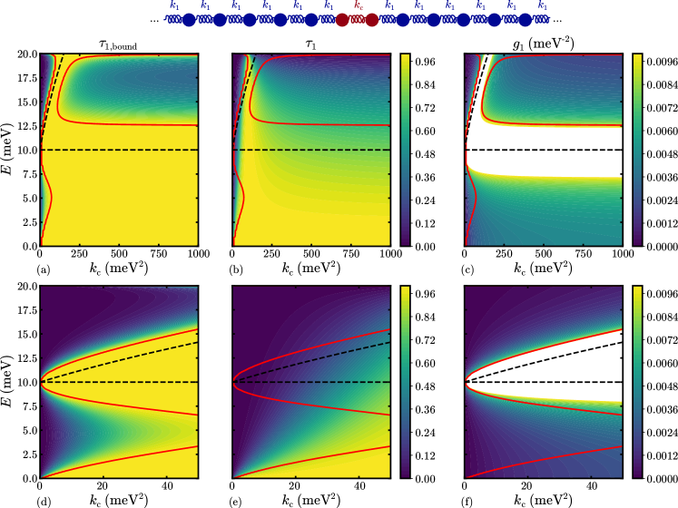
In this section, we apply our limits to the simple but representative system depicted in Fig. 2(a). Specifically, we consider phonon transport in the longitudinal direction in a 1-dimensional (1D) chain, comparing directly to results by Klöckner et al Klöckner et al. (2018), using the same conventions that $\hbar=m=1$, and that the central junction is made of two atoms coupled at strength $k_{\mathrm{c}}$ to each other and at strength $k_{1}$ to the respective leads (which have uniform internal couplings $k_{1}$). Our unit convention means that $\omega$ is in units of $\mathrm{meV}$, while $k_{\mathrm{c}}$ and $k_{1}$ are in units of $\mathrm{meV}^{2}$; in particular, consistent with that work, we set $k_{1}=100\leavevmode\nobreak\ \mathrm{meV}^{2}$ for ease of comparison. The analysis in that prior work shows that dissipation vanishes for $E\geq 2\sqrt{k_{1}}$ and $E=0$, and so we restrict consideration to $E\in(0,2\sqrt{k_{1}})$; additionally, straightforward algebraic manipulations yield the figures of merit, $\zeta_{1}=\zeta_{2}=\frac{2k_{1}^{2}}{E\sqrt{4k_{1}-E^{2}}}$ and $g_{1}=\frac{k_{\mathrm{c}}}{|(E^{2}-(k_{\mathrm{c}}+k_{1}))^{2}-k_{\mathrm{c}}^{2}|}$.

It can be seen in Fig. 2(a–c) that for $k_{\mathrm{c}}=k_{1}$, perfect transmission is possible in actuality, and the bounds reflect this. Such a rate-matching condition corresponds to the “defect” in the central junction no longer behaving distinctly from the leads, so the infinite 1D chain is uniform, and phonons can be perfectly transmitted at any frequency. For $k_{\mathrm{c}}>k_{1}$, although the transmissive efficacy $g_{1}$ need not be particularly large for such combinations of $(E,k_{\mathrm{c}})$, the material response factors $\zeta$ are large enough for the bound to essentially saturate the Landauer limit of unity. With respect to the actual heat transfer, in this regime, the central spring is much stiffer than those of the leads, so low-frequency excitations $E\leq\sqrt{k_{1}}$ perfectly transmit across the rigid central spring, while high-frequency excitations $E>\sqrt{k_{1}}$ largely reflect from the defect, so the actual transmission nearly saturate the bounds too.

Meanwhile, for $k_{\mathrm{c}}<k_{1}$ as seen in Fig. 2(d–f), for which decreasing $k_{\mathrm{c}}$ may be physically interpreted as increasing the distance between the two leads (associating the closer atom to each lead in the junction with that lead), for most combinations of $(E,k_{\mathrm{c}})$, the actual transmission, despite being quite close to zero, nearly saturates our bound. This is because for such small $k_{\mathrm{c}}$, most frequencies will lie far from the resonant modes of the junction in isolation, so the response of the junction is quite small. Only for $E$ close to the values $\{\sqrt{k_{1}},\sqrt{k_{1}+2k_{\mathrm{c}}}\}$ does our bound come close to the Landauer limit of unity while the actual transmission does not: this is because these are the resonant frequencies of the junction in isolation, whereas the actual transmission depends on the response of the junction dressed by the two leads and their dissipations, though the range of frequencies over which this deviation occurs narrows as $k_{\mathrm{c}}$ decreases further.

From this, it can be concluded that the only points where our bounds deviate significantly from the actual transmission are near resonances of the junction in isolation, as that is where the transmissive efficacy diverges whereas the actual transmission depends on the response in the presence of the leads. Otherwise, our bounds come much closer to the actual transmission than the Landauer limits of unity at most combinations of $(E,k_{\mathrm{c}})$.

IV Concluding remarks

We have derived new bounds for heat transfer in arbitrary systems with linear bosonic response, and showed that for particular molecular junction geometries of interest to phonon CHT in the linear regime, these per-channel bounds can not only be much tighter than the per-channel Landauer limits of unity across many frequencies but can actually approach the true transmission eigenvalues. As the only points where our bounds approach the Landauer limits but the actual transmission eigenvalues do not are those corresponding to resonances of the junction in isolation (where dressing by the dissipation of the leads matters more), this suggests that in general, our bounds may be tight when the density of states is relatively low, and that sum rules on the density of states could therefore lead to sum rules for heat transfer integrated over all frequencies, a subject for future work. Additionally, as a particular junction structure defines the transmissive efficacies $g_{\mu}$ while the leads with the couplings to the junction define the material response factors $\zeta$, it should be possible at each frequency to determine for a given junction what $\zeta$ allows for saturation of the bounds, and then explore junction designs to arrive at transmissive efficacies $g_{\mu}$ at each frequency able to come close to saturating the Landauer limits of unity (subject to the aforementioned sum rules), though we leave this to future work too.

Acknowledgments.—The authors thank Riccardo Messina, Philippe Ben-Abdallah, and León Martin for the helpful comments and suggestions. This work was supported by the National Science Foundation under Grants No. DMR-1454836, DMR 1420541, DGE 1148900, the Cornell Center for Materials Research MRSEC (award no. DMR1719875), the Defense Advanced Research Projects Agency (DARPA) under agreement HR00111820046, and the Spanish Ministry of Economy and Competitiveness (MINECO) (Contract No. FIS2017-84057-P). The views, opinions and/or findings expressed herein are those of the authors and should not be interpreted as representing the official views or policies of any institution.

Appendix A Derivation of alternative bounds

In this appendix, we derive alternative bounds to heat transfer that do not rely on any assumptions about the couplings of component 3 to components 1 & 2. As discussed in Venkataram et al. (2020a), the energy transfer spectrum can be written as

$$\Phi=4\leavevmode\nobreak\ \left\lVert\operatorname{Im}(\hat{Z}^{(0)\star}_{2})^{1/2}\hat{Y}_{2,2}\Delta\hat{Z}_{2,1}\hat{Y}_{1}\operatorname{Im}(\hat{Z}^{(0)\star}_{1})^{1/2}\right\rVert_{\mathrm{F}}^{2}$$ (17)

in terms of the Frobenius norm squared $\left\lVert\hat{O}\right\rVert_{\mathrm{F}}^{2}={\rm Tr}\left[\hat{O}^{\dagger}\hat{O}\right]$, having defined the operators $\Delta\hat{Z}_{mn}\equiv-\Delta\hat{Z}_{m,3}\hat{Y}^{(0)}_{3}\Delta\hat{Z}_{3,n}$ for $m,n\in\{1,2\}$, and in terms of these the operators $\hat{Y}_{1}\equiv(\hat{Z}^{(0)}_{1}+\Delta\hat{Z}_{1,1})^{-1}$ and $\hat{Y}_{2,2}\equiv(\hat{Z}^{(0)}_{2}+\Delta\hat{Z}_{2,2}-\Delta\hat{Z}_{2,1}\hat{Y}_{1}\Delta\hat{Z}_{1,2})^{-1}$; we point out that although the operators $\Delta\hat{Z}_{3,n}$ (and its transpose) are real-valued for $n\in\{1,2\}$, the operators $\Delta\hat{Z}_{mn}$ defined above for $m,n\in\{1,2\}$ may in general be complex-valued due to the dependence on $\hat{Y}^{(0)}_{3}$.

Using the definitions in the main text of the relevant quantities $|x_{n}\rangle$, $|F_{n}\rangle$, and $|F^{(0)}_{n}\rangle$ for $n\in\{1,2,3\}$, as well as the definitions of absorption, scattering, and extinction in the main text, it can be seen that for a general external force $|F^{(0)}_{1}\rangle$ on component 1 in the presence of component 3 but not component 2, the scattered power is $\Phi_{\mathrm{sca}}=\frac{\omega}{2}\langle F^{(0)}_{1},(\operatorname{Im}(\hat{Y}_{1})-\hat{Y}_{1}^{\star}\operatorname{Im}(\hat{Z}^{(0)\star}_{1})\hat{Y}_{1})F^{(0)}_{1}\rangle$. Similarly, for a general external force $|F^{(0)}_{\mathrm{A}}\rangle$ on the aggregate of components 1 & 2, the far-field scattering from component 2 (i.e. into component 3) is $\Phi_{\mathrm{sca}}=\frac{\omega}{2}\langle F^{(0)}_{2},(\operatorname{Im}(\hat{Y}_{2,2})-\hat{Y}_{2,2}^{\star}(\operatorname{Im}(\hat{Z}^{(0)\star}_{2})+\Delta\hat{Z}_{2,1}^{\star}\hat{Y}_{1}^{\star}\operatorname{Im}(\hat{Z}^{(0)\star}_{1})\hat{Y}_{1}\Delta\hat{Z}_{1,2})\hat{Y}_{2,2})F^{(0)}_{2}\rangle$. This does not require any further assumptions about the couplings to component 3 because all of these quantities are cast in terms of response functions of components 1 & 2, which are assumed to be disjoint, as opposed to the response functions of the subsets of DOFs of component 3 coupled to each of the other components (which might not be). Thus, the relevant operators which must be positive-semidefinite are $\operatorname{Im}(\hat{Y}_{1})-\hat{Y}_{1}^{\star}\operatorname{Im}(\hat{Z}^{(0)\star}_{1})\hat{Y}_{1}$, $\operatorname{Im}(\hat{Y}_{2,2})-\hat{Y}_{2,2}^{\star}(\operatorname{Im}(\hat{Z}^{(0)\star}_{2})+\Delta\hat{Z}_{2,1}^{\star}\hat{Y}_{1}^{\star}\operatorname{Im}(\hat{Z}^{(0)\star}_{1})\hat{Y}_{1}\Delta\hat{Z}_{1,2})\hat{Y}_{2,2}$, and their respective transposes due to reciprocity.

The remainder of the derivation follows exactly analogously to the main text, with the replacements $\hat{B}_{1}\to\operatorname{Im}(\hat{Z}^{(0)\star}_{1})^{1/2}\hat{Y}_{1}\operatorname{Im}(\hat{Z}^{(0)\star}_{1})^{1/2}$, $\hat{B}_{2}\to\operatorname{Im}(\hat{Z}^{(0)\star}_{2})^{1/2}\hat{Y}_{2,2}\operatorname{Im}(\hat{Z}^{(0)\star}_{2})^{1/2}$, and $\hat{A}\to\operatorname{Im}(\hat{Z}^{(0)\star}_{2})^{1/2}\Delta\hat{Z}_{2,1}\operatorname{Im}(\hat{Z}^{(0)\star}_{1})^{1/2}\hat{B}_{1}\times\hat{B}_{1}^{\star}\operatorname{Im}(\hat{Z}^{(0)\star}_{1})^{1/2}\Delta\hat{Z}_{1,2}^{\star}\operatorname{Im}(\hat{Z}^{(0)\star}_{2})^{1/2}$; these follow all of the same requisite properties as their counterparts in the main text. Therefore, the bound can again be written as $\Phi\leq\Phi_{\mathrm{opt}}\leq\Phi_{\mathrm{L}}$ with $\Phi_{\mathrm{opt}}$ given in (16), redefining notation regarding the singular values for these operators such that $\zeta_{n}=\left\lVert\operatorname{Im}(\hat{Z}^{(0)\star}_{n})^{-1}\right\rVert_{2}$ and $g_{\mu}$ are now the singular values of $\Delta\hat{Z}_{2,1}=-\Delta\hat{Z}_{2,3}\hat{Y}^{(0)}_{3}\Delta\hat{Z}_{3,1}$. Once again, this form of our bound has the benefit of being evaluable even if some DOFs of component 3 are simultaneously coupled to components 1 & 2. Additionally, the material response factors $\zeta_{n}$ depend only on the properties of components 1 & 2 in isolation, without any reference to couplings. However, there are two points that may be practical drawbacks. The first is that the transmissive efficacies $g_{\mu}$ depend on both the coupling strengths and the properties of component 3 in isolation, though these effects can be disentangled by further bounding $g_{\mu}\leq\left\lVert\Delta\hat{Z}_{2,3}\right\rVert_{2}\left\lVert\Delta\hat{Z}_{3,1}\right\rVert_{2}\sigma_{\mu}(\hat{P}(\hat{V}_{2})\hat{Y}^{(0)}_{3}\hat{P}(\hat{V}_{1}))$ as an extension of the steps in the derivation in the main text. The second is that particularly in phonon CHT, a system of broad interest takes components 1 & 2 to be semi-infinite leads, with component 3 being a small junction. This means that the procedure in the main text yields material response factors $\zeta_{n}$ that can be easily computed from small matrices, as the matrices $\Delta\hat{Z}_{3,n}\hat{Y}^{(0)}_{n}\Delta\hat{Z}_{n,3}$ can be computed through decimation or similar procedures; by contrast, the procedure in this appendix requires the full matrices $\operatorname{Im}(\hat{Z}^{(0)\star}_{n})$ for $n\in\{1,2\}$, which are large and might technically vanish unless dissipation is added by hand.

Appendix B Glossary of relevant quantities for bounds on CHT

As the quantities discussed in this manuscript are quite general, it is useful to draw specific correspondences to operators common to nonequilibrium Green’s function analyses of CHT in order to more clearly explain how to compute these bounds to CHT in practice. For reference, the notation we use is generally consistent with notation for phonon CHT in several prior works Bürkle et al. (2015); Klöckner et al. (2016, 2017a, 2017b, 2017c, 2018); analogous bounds can be applied to electron CHT with appropriate replacements of operators. The following is a set of steps that can be used as a “recipe” for computing the bounds on CHT developed in this manuscript.

  1. 1.

    Ensure that all quantities have consistent units. For instance, for consistency with prior works Bürkle et al. (2015); Klöckner et al. (2016, 2017a, 2017b, 2017c, 2018) on phonon CHT, it will be assumed that all spring constants are normalized by the atomic masses and by $\hbar$, such that $K_{ai,bj}=\frac{\hbar^{2}}{m_{a}m_{b}}\frac{\partial^{2}E}{\partial x_{ai}\partial x_{bj}}$, and that the angular frequency $\omega$ will be replaced by the energy $E=\hbar\omega$ as the argument of frequency domain response quantities. Furthermore, the components 1 & 2 will be referred to as leads $n\in\{\mathrm{L},\mathrm{R}\}$, while component 3 will be referred to as the central junction $\mathrm{C}$.

  2. 2.

    At each $E$, compute $\boldsymbol{\Pi}^{\mathrm{r}}_{n}=\boldsymbol{K}_{\mathrm{C}n}\boldsymbol{d}^{\mathrm{r}}_{nn}\boldsymbol{K}_{n\mathrm{C}}$, where $\boldsymbol{d}^{\mathrm{r}}_{nn}=((E+\operatorname{i}\eta)\boldsymbol{1}_{nn}-\boldsymbol{K}_{nn})^{-1}$ is given in terms of an infinitesimal real parameter $\eta$ to yield a finite dissipation in each lead $n$.

  3. 3.

    With this, compute $\zeta_{n}=\left\lVert\operatorname{asym}(\boldsymbol{\Pi}^{\mathrm{r}\dagger-1}_{n})^{-1}\right\rVert_{2}$. That is, compute the standard Hermitian adjoint of the matrix $\boldsymbol{\Pi}^{\mathrm{r}}_{n}$, then take the inverse of that within the subspace of DOFs of the junction $\mathrm{C}$ that are coupled to the given lead $n$, then compute the anti-Hermitian part $\operatorname{asym}(\boldsymbol{\Pi}^{\mathrm{r}\dagger-1}_{n})$ (though note that the anti-Hermitian part is by definition a Hermitian operator), then compute the smallest singular value in that subspace, and set $\zeta_{n}$ equal to the reciprocal of that smallest singular value. This requires nontrivial dissipation, so $\operatorname{asym}(\boldsymbol{\Pi}^{\mathrm{r}}_{n})$ should not vanish.

  4. 4.

    At each $E$, compute $\boldsymbol{d}^{\mathrm{r}}_{\mathrm{CC}}=((E+\operatorname{i}\eta)\boldsymbol{1}_{\mathrm{CC}}-\boldsymbol{K}_{\mathrm{CC}})^{-1}$; note that this is the response of the uncoupled junction, which is not the same as $\boldsymbol{D}^{\mathrm{r}}_{\mathrm{CC}}$.

  5. 5.

    Construct the off-diagonal block $\boldsymbol{P}_{\mathrm{C(R)}}\boldsymbol{d}^{\mathrm{r}}_{\mathrm{CC}}\boldsymbol{P}_{\mathrm{C(L)}}$. That is, extract the off-diagonal block of $\boldsymbol{d}^{\mathrm{r}}_{\mathrm{CC}}$ where the rows correspond to atoms in the central junction $\mathrm{C}$ with nonzero couplings to the right lead $\mathrm{R}$, and the columns correspond to atoms in the central junction $\mathrm{C}$ with nonzero couplings to the left lead $\mathrm{L}$. Note that this assumes that no atoms in the central junction couple simultaneously to both leads, so single-atom junctions cannot be treated as single atoms per se (i.e. the junction needs to be artificially increased in size to include more atoms in the leads until those overlaps disappear).

  6. 6.

    Find the singular values $g_{\mu}$ of this off-diagonal block $\boldsymbol{P}_{\mathrm{C(R)}}\boldsymbol{d}^{\mathrm{r}}_{\mathrm{CC}}\boldsymbol{P}_{\mathrm{C(L)}}$; the label $\mu$ is said to denote the channel. Note that this off-diagonal block is generally not square (i.e. it might not be the case that the numbers of atoms in the junction coupling to each of the leads are the same), but the singular value decomposition (SVD) will always exist and should always yield real nonnegative values (barring unexpected numerical problems).

  7. 7.

    At this $E$, plug the quantities $\zeta_{n}$ and $g_{\mu}$ into (16) for each channel $\mu$ to yield the bound $\Phi_{\mathrm{opt}}$; note the change in labels $n\in\{1,2\}\to\{\mathrm{L},\mathrm{R}\}$.

References

  • Segal and Agarwalla (2016) D. Segal and B. K. Agarwalla, “Vibrational heat transport in molecular junctions,” Annual Review of Physical Chemistry 67, 185–209 (2016), pMID: 27215814, https://doi.org/10.1146/annurev-physchem-040215-112103 .
  • Tian et al. (2012) Z. Tian, K. Esfarjani,  and G. Chen, “Enhancing phonon transmission across a si/ge interface by atomic roughness: First-principles study with the green’s function method,” Phys. Rev. B 86, 235304 (2012).
  • Tian et al. (2014) Z. Tian, K. Esfarjani,  and G. Chen, “Green’s function studies of phonon transport across si/ge superlattices,” Phys. Rev. B 89, 235307 (2014).
  • Bürkle et al. (2015) M. Bürkle, T. J. Hellmuth, F. Pauly,  and Y. Asai, “First-principles calculation of the thermoelectric figure of merit for [2,2]paracyclophane-based single-molecule junctions,” Phys. Rev. B 91, 165419 (2015).
  • Klöckner et al. (2017a) J. C. Klöckner, R. Siebler, J. C. Cuevas,  and F. Pauly, “Thermal conductance and thermoelectric figure of merit of ${\mathrm{c}}_{60}$-based single-molecule junctions: Electrons, phonons, and photons,” Phys. Rev. B 95, 245404 (2017a).
  • Klöckner et al. (2017b) J. C. Klöckner, M. Matt, P. Nielaba, F. Pauly,  and J. C. Cuevas, “Thermal conductance of metallic atomic-size contacts: Phonon transport and wiedemann-franz law,” Phys. Rev. B 96, 205405 (2017b).
  • Klöckner et al. (2017c) J. C. Klöckner, J. C. Cuevas,  and F. Pauly, “Tuning the thermal conductance of molecular junctions with interference effects,” Phys. Rev. B 96, 245419 (2017c).
  • Luo and Chen (2013) T. Luo and G. Chen, “Nanoscale heat transfer - from computation to experiment,” Phys. Chem. Chem. Phys. 15, 3389–3412 (2013).
  • Cahill et al. (2014) D. G. Cahill, P. V. Braun, G. Chen, D. R. Clarke, S. Fan, K. E. Goodson, P. Keblinski, W. P. King, G. D. Mahan, A. Majumdar, H. J. Maris, S. R. Phillpot, E. Pop,  and L. Shi, “Nanoscale thermal transport. ii. 2003-2012,” Applied Physics Reviews 1, 011305 (2014)http://dx.doi.org/10.1063/1.4832615 .
  • Pop (2010) E. Pop, “Energy dissipation and transport in nanoscale devices,” Nano Research 3, 147–169 (2010).
  • Cui et al. (2017) L. Cui, W. Jeong, S. Hur, M. Matt, J. C. Klöckner, F. Pauly, P. Nielaba, J. C. Cuevas, E. Meyhofer,  and P. Reddy, “Quantized thermal transport in single-atom junctions,” Science 355, 1192–1195 (2017)https://science.sciencemag.org/content/355/6330/1192.full.pdf .
  • Mosso et al. (2017) N. Mosso, U. Drechsler, F. Menges, P. Nirmalraj, S. Karg, H. Riel,  and B. Gotsmann, “Heat transport through atomic contacts,” Nature nanotechnology 12, 430 (2017).
  • Cui et al. (2019) L. Cui, S. Hur, Z. A. Akbar, J. C. Klöckner, W. Jeong, F. Pauly, S.-Y. Jang, P. Reddy,  and E. Meyhofer, “Thermal conductance of single-molecule junctions,” Nature , 1–1 (2019).
  • Mosso et al. (2019) N. Mosso, H. Sadeghi, A. Gemma, S. Sangtarash, U. Drechsler, C. Lambert,  and B. Gotsmann, “Thermal transport through single-molecule junctions,” Nano Letters 19, 7614–7622 (2019), pMID: 31560850, https://doi.org/10.1021/acs.nanolett.9b02089 .
  • Cuevas et al. (1998) J. C. Cuevas, A. L. Yeyati,  and A. Martín-Rodero, “Microscopic origin of conducting channels in metallic atomic-size contacts,” Phys. Rev. Lett. 80, 1066–1069 (1998).
  • Mingo and Yang (2003) N. Mingo and L. Yang, “Phonon transport in nanowires coated with an amorphous material: An atomistic green’s function approach,” Phys. Rev. B 68, 245406 (2003).
  • Dhar and Roy (2006) A. Dhar and D. Roy, “Heat transport in harmonic lattices,” Journal of Statistical Physics 125, 801–820 (2006).
  • Klöckner et al. (2016) J. C. Klöckner, M. Bürkle, J. C. Cuevas,  and F. Pauly, “Length dependence of the thermal conductance of alkane-based single-molecule junctions: An ab initio study,” Phys. Rev. B 94, 205425 (2016).
  • Klöckner et al. (2018) J. C. Klöckner, J. C. Cuevas,  and F. Pauly, “Transmission eigenchannels for coherent phonon transport,” Phys. Rev. B 97, 155432 (2018).
  • Zhang et al. (2018) Z.-Q. Zhang, J.-T. Lü,  and J.-S. Wang, “Energy transfer between two vacuum-gapped metal plates: Coulomb fluctuations and electron tunneling,” Phys. Rev. B 97, 195450 (2018).
  • Sadasivam et al. (2017) S. Sadasivam, U. V. Waghmare,  and T. S. Fisher, “Phonon-eigenspectrum-based formulation of the atomistic green’s function method,” Phys. Rev. B 96, 174302 (2017).
  • Dubi and Di Ventra (2011) Y. Dubi and M. Di Ventra, “Colloquium: Heat flow and thermoelectricity in atomic and molecular junctions,” Rev. Mod. Phys. 83, 131–155 (2011).
  • Venkataram et al. (2020a) P. S. Venkataram, R. Messina, J. Cuevas, P. Ben-Abdallah,  and A. W. Rodriguez, “Mechanical relations between conductive and radiative heat transfer,”   (2020a), arXiv:2005.14342 .
  • Molesky et al. (2020) S. Molesky, P. S. Venkataram, W. Jin,  and A. W. Rodriguez, “Fundamental limits to radiative heat transfer: Theory,” Phys. Rev. B 101, 035408 (2020).
  • Venkataram et al. (2020b) P. S. Venkataram, S. Molesky, W. Jin,  and A. W. Rodriguez, “Fundamental limits to radiative heat transfer: The limited role of nanostructuring in the near-field,” Phys. Rev. Lett. 124, 013904 (2020b).
  • Mirsky (1975) L. Mirsky, “A trace inequality of john von neumann,” Monatshefte für Mathematik 79, 303–306 (1975).
  • Miller et al. (2016) O. D. Miller, A. G. Polimeridis, M. T. H. Reid, C. W. Hsu, B. G. DeLacy, J. D. Joannopoulos, M. Soljačić,  and S. G. Johnson, “Fundamental limits to optical response in absorptive systems,” Opt. Express 24, 3329–3364 (2016).
  • Hogben (2013) L. Hogben, Handbook of linear algebra (Chapman and Hall/CRC, 2013).