Continuous-variable assisted thermal quantum simulation

Abstract

Simulation of a quantum many-body system at finite temperatures is crucially important but quite challenging. Here we present an experimentally feasible quantum algorithm assisted with continuous-variable for simulating quantum systems at finite temperatures. Our algorithm has a time complexity scaling polynomially with the inverse temperature and the desired accuracy. We demonstrate the quantum algorithm by simulating finite temperature phase diagram of the Kitaev model. It is found that the important crossover phase diagram of the Kitaev ring can be accurately simulated by a quantum computer with only a few qubits and thus the algorithm may be readily implemented on current quantum processors. We further propose a protocol implementable with superconducting or trapped ion quantum computers.

Introduction.– Simulation of quantum many-body systems has been an incentive for building quantum computers Feynman (1982). Recent advances of scaling-up quantum processors enable us to simulate steady states and dynamics of a quantum system at zero temprature to a larger size Barends et al. (2015); Bernien et al. (2017); Kandala et al. (2017); Zhang et al. (2017), and remarkably, to make a simulation of quantum phase transition to be a reality Islam et al. (2011); Zhang et al. (2017). However, simulation of a quantum many-body system at finite temperatures is even more challenging as the state in a quantum computer is usually a pure quantum state, while simulating a quantum system at finite temperatures requires to simulate a kind of mixed states, namely quantum thermal (Gibbs) states. The relevance of thermal states is ubiquitous, and its simulaiton is not only important for physics itself, such as understanding high-Tc superconductivity Lee et al. (2006) , but also can provide quantum speedup for optimization Van Apeldoorn et al. (2017).

Thermal quantum simulation (TQS) requires a well control of both quantum coherence and temperature, which challenges the current quantum platforms. A quantum algorithm based on quantum phase estimation may involve a large number of auxiliary qubits and complicated quantum circuits, which is not suitable for near-term quantum simulators Terhal and DiVincenzo (2000); Poulin and Wocjan (2009); Temme et al. (2011); Riera et al. (2012). Recent hybrid quantum-classical variational algorithms require less quantum resource and are feasible in implementation  Wu and Hsieh (2019); Verdon et al. (2019); Liu et al. (2019); Chowdhury et al. (2020); Wang et al. (2020), but it should be trained for each Hamiltonian at every temperature and thus is not a general solution. Moreover, it waits for a guarantee of quantum advantages in time complexity.

An alternative way is to use continuous variables  (CV and also called qumode) for encoding and processing high-density information by exploiting its infinite dimensional Hilbert space Weedbrook et al. (2012); Lau et al. (2017). Notably, a hybrid approach of incorporating both qubits and qumodes has been shown to have a potential advantage to make the best-of-both-worlds Furusawa and Van Loock (2011); Andersen et al. (2015); Liu et al. (2016); Gan et al. . Moreover, the mainstream platforms of quantum computers often have naturally existing continuous variables, such as motional modes of trapped ions Leibfried et al. (2003); Monroe and Kim (2013) and cavity modes of superconducting circuits Wallraff et al. (2004); Paik et al. (2011); Devoret and Schoelkopf (2013), making a hybrid variable approach physical realizable. This may enable us to design hybrid-variable quantum algorithms for TQS with both quantum advantage and feasible physical implementation.

In this paper, we present a quantum algorithm for thermal quantum simulation assisted with an auxiliary qumode, which has a time complexity scaling polynomially with the inverse temperature $\beta$ and the desired accuracy $\epsilon$. The algorithm converts thermal information, encoded in the CV resource state parameterized with $\beta$, into temperature of the quantum system. Moreover, by revealing an equivalence relation of the quantum algorithm, we further propose adaptive TQS, allowing TQS at varied $\beta$ with a proper-chosen resource state, which enables flexibility of algorithm design in practice. To show the power of adaptive TQS, we consider thermal states of two textbook models, the quantum Ising model Sachdev and Kitaev ring Kitaev (2001), in the quantum critical regime, and demonstrate our algorithm can accurately determine the crossover temperature. This indicates an interplay between quantum and thermal fluctuations, which underlines the quantum criticality at finite temperatures, can be faithfully captured. An intriguing result here is that the important crossover phase diagram of the Kitaev model in periodic condition (Kitaev ring) can be accurately simulated by a quantum computer with only a few qubits and thus the algorithm may be readily implemented on current quantum processors. We also propose an experimental protocol implementable with a superconducting or trapped ion quantum computer. Our work opens a new avenue for simulating finite temperature quantum systems by exploiting the power of continuous variables.

Thermal quantum simulation. Consider a quantum system described by a Hamiltonian $H$, which can be mapped to a quantum computer with $N$ qubits. The energies and eigenstates of the Hamiltonian governed by the Schrodinger equation $H|u_{n}\rangle=E_{n}|u_{n}\rangle$ ($n=0,1,...,D-1$,where $D=2^{N}$). At a finite temperature $T=1/\beta$, the system in equilibrium is in a quantum thermal state $\rho(\beta)=e^{-\beta H}/Z(\beta)$, where $Z(\beta)=\text{Tr}e^{-\beta H}$ is the partition function. Our goal is to prepare a pure quantum state $|\psi(\beta)\rangle$ in an enlarger Hilbert space which has the property $\rho(\beta)=\text{Tr}_{A}|\psi(\beta)\rangle\langle\psi(\beta)|$, where $\text{Tr}_{A}$ denotes the partial trace of some ancillary degrees of freedom addressed later. One can verify that, partial trace of the second partite of the thermofield double (TFD) state defined as

$$|\psi(\beta)\rangle=\sum_{n}\frac{e^{-\beta E_{n}/2}}{\sqrt{\mathcal{Z}(\beta)}}|u_{n}\rangle\otimes|u^{*}_{n}\rangle$$ (1)

is just $\rho(\beta)$. We propose a quantum process as follows,

$$|\psi(\beta)\rangle=\sqrt{\mathcal{C}}e^{-\beta H/2}\otimes I|\psi(0)\rangle,$$ (2)

where $\mathcal{C}$ is a normalization factor. Here $|\psi(0)\rangle=\frac{1}{\sqrt{D}}\sum_{n}|n\rangle\otimes|n\rangle$ is an infinite temperature TFD which can be written as a product of N copies of Bell state (see Supplementary Material (SM) for a derivation), and thus is easy to prepare. The central task is then to construct $e^{-\beta H/2}$.

We introduce an auxiliary qumode to represent a nonunitary $e^{-\beta H/2}$ as an integral of unitaries Lau et al. (2017); Arrazola et al. (2019); Zhang et al. (2019, 2020), which extends the linear-combination-of-unitaries to the case of CV Gui-Lu (2006); Childs et al. (2017); Van Apeldoorn et al. (2017); Gilyen et al. (2018); Arrazola et al. (2019). Note that

$$e^{-\beta h/2}=\int_{-\infty}^{\infty}dpR(\beta,p)e^{-ihp},~{}~{}R(\beta,p)=\frac{2}{\pi}\frac{\beta}{\beta^{2}+4p^{2}}$$ (3)

holds for $h\geq 0$. It implies that we shall add a constant to $H$ to guarantee a nonnegative ground state energy in the algorithm. Then in the basis $\{|u_{n}\rangle\}$ that $H$ is diagonal, one can verify that

$$e^{-\beta H/2}=\int_{-\infty}^{\infty}dpR(\beta,p)e^{-iHp}\propto\langle 0_{q}|e^{-iH\hat{p}}|R(\beta)\rangle,$$ (4)

where $|R(\beta)\rangle=\sqrt{\beta\pi}\int_{-\infty}^{\infty}dpR(\beta,p)|p\rangle_{p}$. Here we denote $|p\rangle_{p}$ ($|q\rangle_{q}$) as basis of continuous variable quadrature $\hat{p}$ ($\hat{q}$). Eq. (4) shows a scheme that the nonunitary operator $e^{-\beta H/2}$ can be implemented on a quantum computer, assisted with an ancillary qumode. The qumode is prepared at $|R(\beta)\rangle$, evolves jointly with the system by $e^{-iH\hat{p}}$, and is finally projected onto $|0\rangle_{q}$. As the information related to temperature is encoded in $|R(\beta)\rangle$, we may call it as a resouce state.

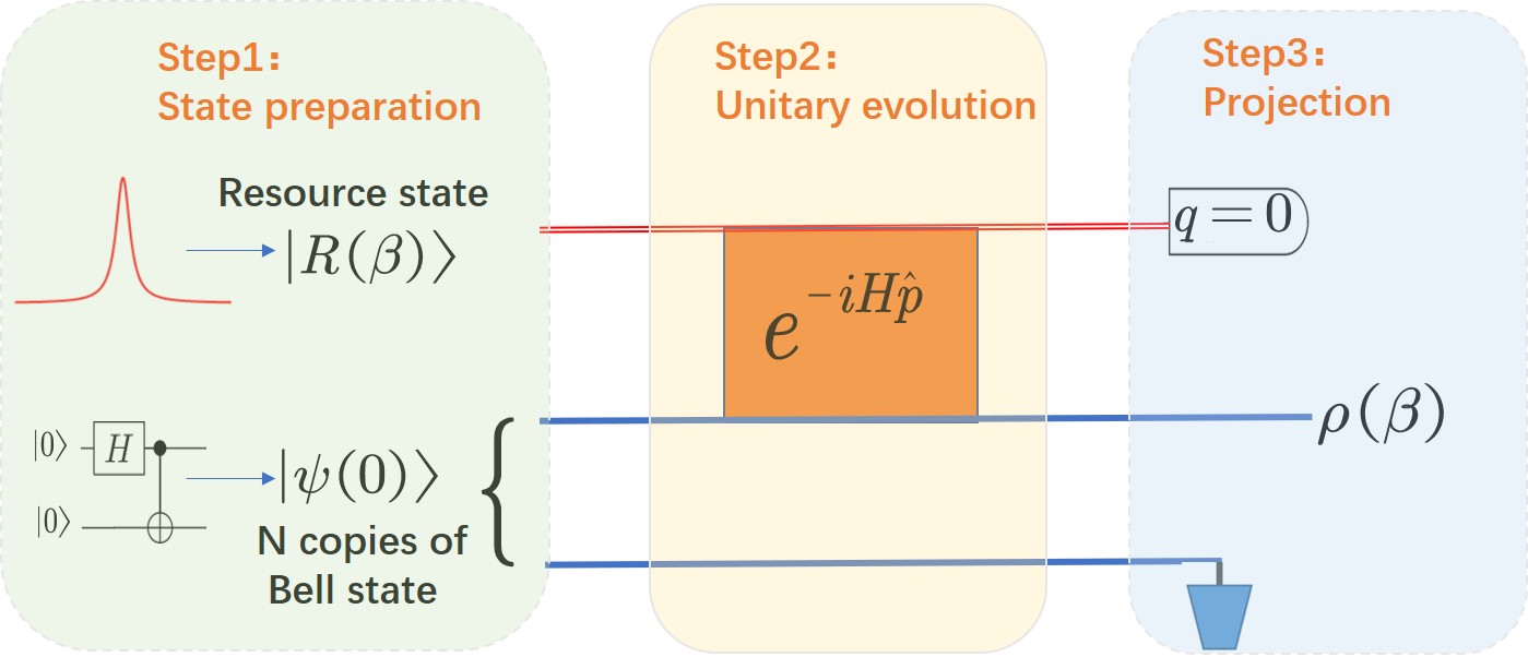
Figure 1: An illustration of preparing quantum thermal state $\rho(\beta)$ from N copies of Bell states, through coupling the system with a qumode by unitary evolution $e^{-iH\hat{p}/2}$. The qumode is initialed at the resource state $|R(\beta)\rangle$ and is finally projected onto $|0\rangle_{q}$. Thermal state $\rho(\beta)$ is obtained by discarding (tracing out) the additional $N$ ancillary qubits.

Quantum algorithm.– We now present the procedure of quantum algorithm for preparing thermal quantum simulation. The quantum algorithm is probabilistic since it postselects the quadrature $\hat{q}$ to zero. In practice, the measurement should have a finite precision, which reduces the accuracy while raises the success rate. We model this effect by projecting to a squeezing state $|0,s\rangle=s^{-\frac{1}{2}}\pi^{-\frac{1}{4}}\int dp|p\rangle_{p}e^{-p^{2}/2s^{2}}$, which squeezes the quadrature $\hat{q}$ by a factor $s$. The quantum algorithm, as illustrated in Fig. 1, has three steps:

1. State preparation. Prepare N copies of Bell states, $|\psi(0)\rangle=\prod_{i=1}^{N}B_{i,i+N}$, where $B_{i,i+N}=\frac{1}{\sqrt{2}}(|0_{i}0_{i+N}\rangle+|1_{i}1_{i+N}\rangle)$ is a Bell state. A qumode is initialized in a resource state $|R(\beta)\rangle$. The total system is in a state $|\Psi_{0}\rangle=|\psi(0)\rangle\otimes|R(\beta)\rangle$. Therefore, to simulate a Hamiltonian $H$ which is encoded in $N$ qubits, our scheme needs $2N$ qubits and one qumode.

2. Unitary evolution. A constant is added to $H$ to make positivity of the spectrum. then the unitary evolution $e^{-iH\hat{p}}\otimes I$ is implemented and it couples the system with the qumode. The unitary can be decomposed with Trotter-Suzuki formula, which will be discussed later. The state turns to be

   $$|\Psi_{1}\rangle=\sum_{n}\int_{-\infty}^{\infty}dp\phi_{n}(\beta,p)|u_{n}\rangle\otimes|u^{*}_{n}\rangle\otimes|p\rangle_{p},$$ (5)

   where $\phi_{n}(\beta,p)=\sqrt{\frac{\beta\pi}{D}}R(\beta,p)e^{-E_{n}p}$.

3. Projection. Project the qumode onto a squeezing state $|0,s\rangle$, the unnormalized final state (discarding the qumode) is

   $$|\tilde{\psi}(\beta)\rangle=\sum_{n}a(E_{i},\beta,s)|u_{n}\rangle\otimes|u^{*}_{n}\rangle,$$ (6)

   where $a(E,\beta,s)=s^{-\frac{1}{2}}\pi^{-\frac{1}{4}}\int_{-\infty}^{\infty}dp\phi_{n}(\beta,p)e^{-\frac{p^{2}}{2s^{2}}}$. The success rate is $O(\frac{\mathcal{Z}(\beta)}{sD})$.

Note at $s\rightarrow\infty$ limit, $a(E,\beta,s)\propto e^{-\beta E/2}$, which exactly equals to the quantum thermal state at an inverse temperature $\beta$.

One issue of the quantum algorithm is that the resource state can not be produced for free, e.g., $R(\beta\rightarrow 0)$ and $R(\beta\rightarrow\infty)$ can not be efficiently prepared since they are infinitely squeezed. To solve this problem, we reveal an equivalent relation of the quantum algorithm, which says that $\rho(\beta)$ can be simulated with different pairs of resource states and unitary evolutions, namely

$$\left(R(\beta_{0}),e^{-iH\hat{p}\frac{\beta}{\beta_{0}}}\right)\mapsto\rho(\beta),$$ (7)

where $\beta_{0}$ is adjustable. The equivalent relation is a direct consequence of an invariance under $\beta\rightarrow a\beta$ and $H\rightarrow H/a$ in Eq. (4).

The equivalent relation allows us to use a fixed resource state to simulate the thermal state at varied $\beta$, which we call as adaptive TQS. From the perspective of quantum resource theory Chitambar and Gour (2019), the equivalent relation may reveal a conversion between static resource (preparing resource state) and dynamical resource (constructing unitary $e^{-iH\hat{p}}$) and their trade-off for thermal quantum simulation. It enriches the flexibility and feasibility of algorithmic implementation , as difficulties of resource state preparation and Hamiltonian evolution vary on different quantum platforms.

Time complexity.– We give a runtime analysis for a relative error $\epsilon$ in the partition function. As it is not practical to ignore the cost of preparing resource state (e.g., at $\beta\rightarrow 0,\infty$ limits), we consider adaptive TQS with a resource state $|R(\beta_{0})\rangle$ that is easy to prepare. The runtime then relies on the circuit complexity of constructing the unitary operator $e^{-iH\hat{p}\beta/\beta_{0}}$ and the success rate.

For a Hamiltonian $H=\sum_{i=1}^{M}c_{i}H_{i}$ with local terms, one can refer to Trotter-Suzuki formula Lloyd (1996) to decompose $e^{-iH\hat{p}\beta/\beta_{0}}$. Typically, it includes terms like evolutions of $\sigma^{\alpha}_{i}\hat{p},\sigma^{\alpha}_{i}\sigma^{\gamma}_{i+1}\hat{p}$ ($\alpha,\gamma=x,y,z$), which can be viewed as parity-dependent displacement operator and can be decomposed as basic gates of qubits and a hybrid gate $e^{i\theta\sigma^{x}\hat{p}}$ (see SM). The circuit complexity is $O(M^{3}\epsilon^{-1}\beta^{2})$, and may be improved with more advanced techniques  Low and Chuang (2017); Campbell (2019); Childs et al. (2019). For a precision $\epsilon$, the squeezing factor should be $s=O(\epsilon^{-\frac{1}{2}})$. Using amplitude amplification G. Brassard and Tapp (2002), the success rate becomes $O(\sqrt{\frac{\mathcal{Z}(\beta)}{sD}})$, and the algorithm should be run repeatedly with $O(\sqrt{\frac{D}{\mathcal{Z}(\beta)}}\epsilon^{-\frac{1}{4}})$ times. In total, the time complexity is $O(\sqrt{\frac{D}{\mathcal{Z}(\beta)}}M^{3}\beta^{2}\epsilon^{-\frac{5}{4}})$, which improves polynomially from methods using quantum phase estimation Poulin and Wocjan (2009). In addition, we found that the quantum algorithm gives a bound from below for the partition function (see SM).

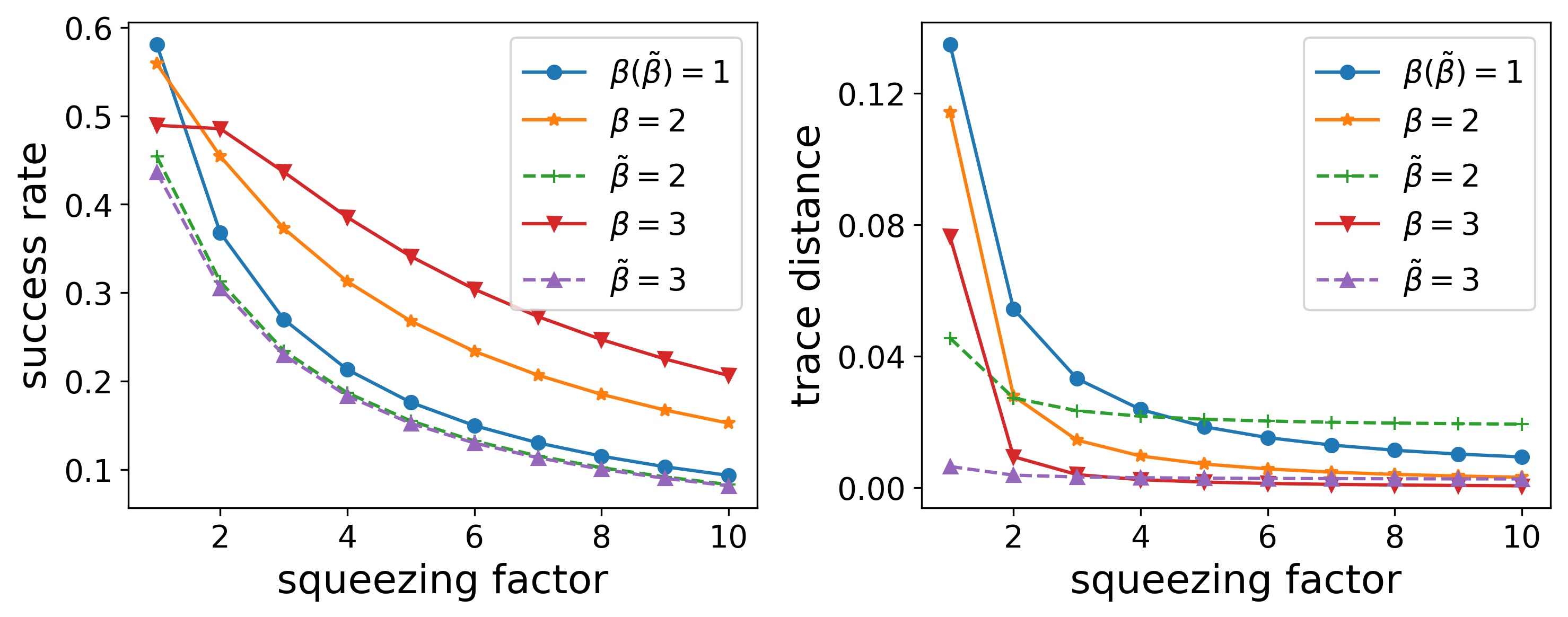
Figure 2: Performance of preparing thermal states of single qubit with two different approaches: $\beta$ ($\tilde{\beta}$) stands for results from TQS (adaptive TQS).

Demonstration with single qubit.– To warm up, we simulate thermal state of a single qubit to highlight some features of the quantum algorithm. For the numeral simulation, we develop a classical simulator for hybrid-variable quantum computing based on the open-source Qutip Johansson et al. (2013). The Hamiltonian is $H=g(\sigma_{x}+c)$ (here $g>0$ and $c=1$ enforces all eigenvalues are nonnegative). After initialing the cavity mode into a resource state and preparing a Bell state, an unitary $e^{-ig(\sigma^{x}+1)\hat{p}t}$ performs on the cavity mode and the system qubit, and finally the cavity mode is squeezed and projected onto zero photon. We use two approaches for preparing thermal states at $\beta=1,2,3$. The first fixes $t=1$ and uses resource states $|R(\beta)\rangle$ with $\beta=1,2,3$, respectively. The second is adaptive TQS, fixing the resource state $|R(\beta=1)\rangle$ and using $t=1,2,3$, respectively. Due to finite squeezing at the projection, those simulated thermal states can only approximate the exact thermal states. We use trace distance to measure the precision, $d_{r}(\beta)=\frac{1}{2}\text{Tr}|\tilde{\rho}(\beta)-\rho(\beta)|$. In Fig. 2, we can see that trace distances decrease rapidly with an increase of squeezing factor, at the cost of decreasing success rate, which are expected. Using adaptive TQS, the increasing of precision can be faster, and the trace distance can be small even at small $s$. Moreover, a moderate truncation of phonon number (e.g., up to $7$ even-number Fock states) can reach a good precision (see SM). The above results indicate that we can use an adaptive approach with approximated resource state for thermal quantum simulation.

Simulation of the finite-temperature phase diagram.– We now consider our TQS with two textbook models, the Kitaev ring (a spinless p-wave superconductor)  Kitaev (2001) and quantum Ising model  Sachdev . The Hamiltonian of the Kitaev ring reads

$$H_{K}=-J\sum_{i=1}^{L}(c_{i}^{\dagger}c_{i+1}+c_{i}^{\dagger}c_{i+1}^{\dagger}+h.c.)-\mu\sum_{i=1}^{L}c_{i}^{\dagger}c_{i},$$ (8)

where fermionic operators $c_{L+1}=c_{1}$ as we consider the periodic condition. The model has a topological phase transition at $\lambda_{K}\equiv\mu/2J=1$. Using Jordan-Wigner transformation, $c_{i}=\prod_{j=1}^{i-1}\sigma_{j}^{z}\sigma_{i}^{-},~{}c_{i}^{\dagger}=\sigma_{i}^{+}\prod_{j=1}^{i-1}\sigma_{j}^{z},~{}c_{i}^{\dagger}c_{i}=\frac{1}{2}(\sigma_{i}^{z}-1)$, the Hamiltonian of the Kitaev ring can be mapped into a spin model

$$H_{S}=-h\sum_{i}^{L}\sigma_{i}^{z}-J\sum_{i}^{L-1}\sigma_{i}^{x}\sigma_{i+1}^{x}-J\sigma_{1}^{y}P_{L}\sigma_{L}^{y}+E_{0},$$ (9)

where $h=-\frac{\mu}{2}$, $P_{L}=\prod_{i=2}^{L-1}\sigma_{i}^{z}$ is a string operator, $E_{0}$ is added for assuring nonnegative spectrum (which is demanded for the quantum algorithm). The spin model $H_{S}$ become the quantum Ising model if $\sigma_{1}^{y}P_{L}\sigma_{L}^{y}$ is replaced by $\sigma_{L}^{x}\sigma_{1}^{x}$, and it has a phase transition at $\lambda_{S}\equiv h/J=1$. This difference of the Ising and Kitaev models has a big effect on the quantum criticality at small sizes, as addressed below. The finite-temperature phase diagrams of these two models in the infinite lattice size are the same, which have an important V-shape crossover structure Sachdev as shown in Fig. 3.

From numeral calculation (see SM for details), it is shown that almost $L\approx 80$ qubits is required for the quantum Ising chain to show well shaped crossover temperatures, as seen in Fig 3, and $L$ should be larger closer to the QPT point. For the Kitaev ring, in contrast, the temperature crossovers are very close in shape for a quite large range even for small $L$. The subtle lies in that Kitaev ring always has an energy gap $\Delta=J|1-\lambda_{K}|$, while the quantum Ising model will have low-lying in-gap states when $\lambda_{S}<1$, leading to small crossover temperatures for $\lambda_{S}<1$, which is obvious for $L=10,20$. Thus, we refer to a small size Kitaev ring for simulating finite-temperature phase diagram with quantum computers.

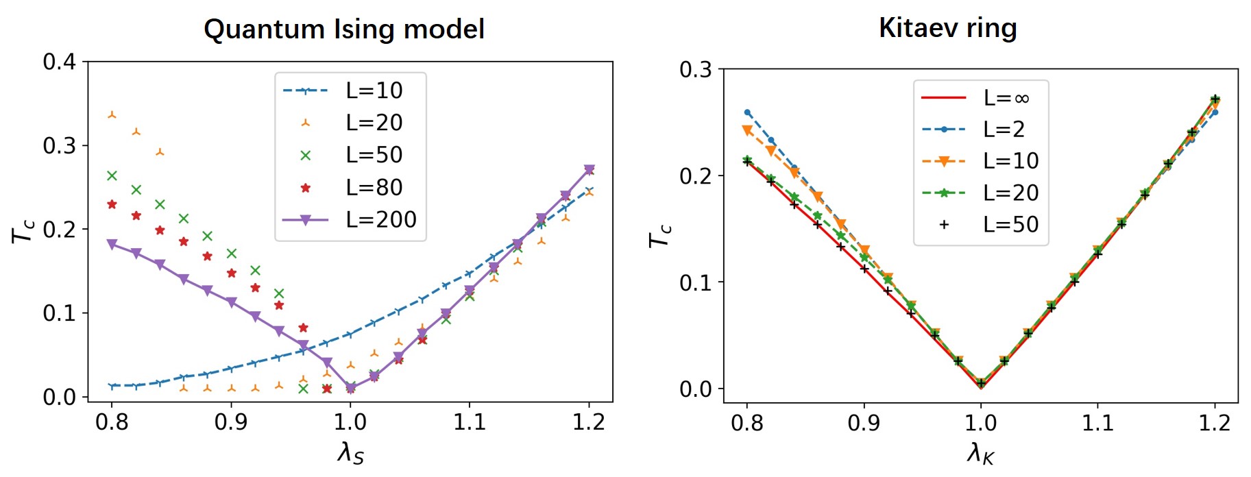
Figure 3: Finite temperature phase diagram of the one-dimensional Kitaev ring and quantum Ising model.

To address the feasibility of the physical implementation, we adopt adaptive TQS for simulating thermal states of the Kitaev ring, using a resource state $|R(\beta=4)\rangle$ and a squeezing factor $s=10$. The crossover temperature for each $\lambda_{K}$ is determined by the temperature that maximizes the magnetic susceptibility $\chi_{m}$ (corresponding to fluctuation of fermion number in the Kitaev ring), which can be obtained by measuring the magnetization $\mathcal{M}=\frac{1}{L}\sum_{i}\text{Tr}\rho(\beta)\sigma_{i}^{z}$ and then calculating the magnetic susceptibility $\chi_{m}=\frac{\partial\mathcal{M}}{\partial h}$ using a finite difference. The result is shown in Fig. 4. For $L=2$, we compare results of different truncation for the resource state ($N_{c}$ is the number of Fock basis of even-number photons), and it can be seen that the $V$-shape crossover temperature approaches the exact one when increasing $N_{c}$. We also simulate $L=2,3,4,5$, which demonstrates very close crossover temperatures. Therefore, a remarkable advantage of our quantum algorithm is that observation of the important crossover temperature phase diagram of the Kitaev ring needs only a few qubits.

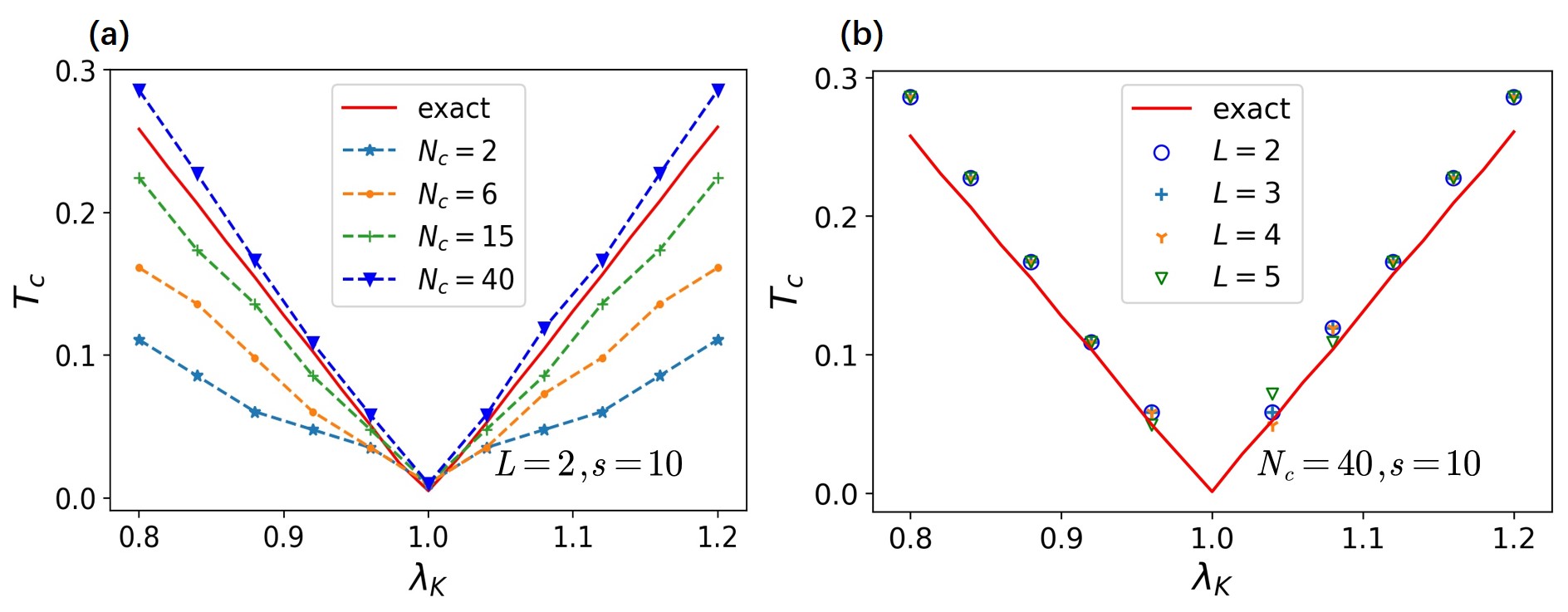
Figure 4: Simulation of crossover temperature for the Kitaev ring in the quantum critical regime with adaptive TQS. (a). Crossover temperatures that use different truncating of photon number $N_{c}$ for the resource state $|R(\beta=4)\rangle$.(b).Crossover temperature for different lattice size, $L=2,3,4,5$.

Experimental realization.– We now discuss physical implementation of the quantum algorithm, which relies on hybrid variable quantum computing. Promising candidates include trapped ions Leibfried et al. (2003); Zhu et al. (2006); Häffner et al. (2008); Monroe and Kim (2013); Zhang et al. (2018) and superconducting circuits Krastanov et al. (2015); Li et al. (2017); Hofheinz et al. (2008); Heeres et al. (2015); Li et al. (2017); Hu et al. (2019); Song et al. (2019), etc. We take superconducting circuit system as an example, for their well controllable CV cavity mode and its coupling to the qubits. The scheme can be straightforwardly used in trapped ion quantum computer.

Firstly, the resource state can be expanded in a Fock space, $|R(\beta)\rangle=\sum_{n=0}^{\infty}r_{n}|2n\rangle$, where $r_{n}=\int_{-\infty}^{\infty}dq\sqrt{\frac{\beta}{2}}e^{-\beta|q|/2}H_{2n}(q)e^{-\frac{q^{2}}{2}}$ and $H_{n}(q)$ is the $n$-th order Hermite function. With a truncation of photon number, the state can be prepared in a cavity by superposing even-number photons. This can be achieved with a sequence of qubit rotation and Jaynes-cumming type qubit-cavity coupling  Law and Eberly (1996); Hofheinz et al. (2009), or using the number-dependent arbitrary phase gate and displacement operator in the dispersive regime Heeres et al. (2015); Wang et al. (2017). Note that resource states around $\beta=2$ can be approximated with a few components of small number photons, and are feasible in both approaches. Thus, we can chose one such resource state and use it for adaptive TQS. Secondly, construction of $e^{-iH\hat{p}t}$ can be compiled into basic qubit gates and only one hybrid variable gate $e^{i\theta\sigma^{x}\hat{p}}$, as discussed before. All are standard quantum operations in superconducting circuit system, and remarkably, the hybrid gate $e^{i\theta\sigma^{x}\hat{p}}$ can be readily realized in the strong coupling limit  Niemczyk et al. (2010); Forn-Díaz et al. (2017, 2019). Thirdly, projection onto a squeezing state $|0,s\rangle$ can be implemented by first performing a squeezing on the CV mode, and then post-selecting the CV mode to the vacuum state (zero photon state). Further, we can measure the system to access the thermal state by quantum state tomography, or studying quantum statistical mechanism by measuring physical quantities, such as heat capacity, magnetic susceptibility, etc. As for the Kitaev ring, we note that evolution of nonlocal term $\sigma_{1}^{y}P_{L}\sigma_{L}^{y}\hat{p}$ can be constructed efficiently (see SM). Thus, all above well-developed quantum operations can render a feasible implementing protocol for thermal quantum simulation of the Kitaev ring, in order to illuminate the novel quantum critical regime on small quantum processors.

Summary.– We have proposed a quantum algorithm for thermal quantum simulation assisted with an auxiliary CV resource state. We have confirmed its power by simulating finite-temperature phase diagram of the Kitaev ring, and found that the important crossover phase diagram of the model can be accurately determined by a quantum computer with only a few qubits. Thus, our work may pave the way for studying finite temperature quantum systems in experiments.

Appendix A Supplementary Material

Appendix B Thermofield double state.

We prove that the purified thermal state at finite temperatures can be written as $N$ pairs of Bell states. Denote $\{E_{n}\}$ and $\{|u_{n}\rangle\}$ ($n=0,1,...,2^{N}-1$) as eigenvalues and eigenstates for a Hamiltonian $H$ which can be encoded with $N$ qubits. The system of $H$ at infinite temperatures is described by a complete mixed state. To purify this complete mixed state, we use a thermofield double (TFD) state at infinite temperatures,

$$|\psi(\beta=0)\rangle\equiv\frac{1}{\sqrt{D}}\sum_{n}|u_{n}\rangle\otimes|u^{*}_{n}\rangle=\frac{1}{\sqrt{D}}\sum_{n}|n\rangle\otimes|n\rangle,$$ (10)

where $D=2^{N}$ is the dimension of Hilbert space. We now prove the equation. Note that both $\{|u_{n}\rangle\}$ and $\{|n\rangle\}$ form a complete set of basis for the Hilbert space of $N$ qubits, we can find an unitary transformation that $|u_{n}\rangle=\sum_{n}U_{nm}|m\rangle$. Then,

$$\sum_{n}|u_{n}\rangle\otimes|u^{*}_{n}\rangle = \sum_{nmm^{\prime}}U_{nm}U^{*}_{nm^{\prime}}|m\rangle\otimes|m^{\prime}\rangle$$ (11)

$$= \sum_{mm^{\prime}}\delta_{mm^{\prime}}|m\rangle\otimes|m^{\prime}\rangle$$

$$= \sum_{n}|n\rangle\otimes|n\rangle$$

We prove that $|\psi(0)\rangle=\prod_{i=1}^{N}B_{i,i+N}$, where $B_{i,i+N}=\frac{1}{\sqrt{2}}(|0_{i}0_{i+N}\rangle+|1_{i}1_{i+N}\rangle)$. With a binary expression $n=n_{1}n_{2}..,n_{N}$ ($n_{i}=0,1$), we can write,

$$|\psi(\beta=0)\rangle = \frac{1}{\sqrt{D}}\sum_{n}|n\rangle\otimes|n\rangle$$ (12)

$$= \frac{1}{\sqrt{D}}\sum_{n_{1}n_{2}...n_{N}}|n_{1}n_{2}...n_{N}\rangle\otimes|n_{1}n_{2}...n_{N}\rangle$$

$$= \frac{1}{\sqrt{D}}\prod_{i=1}^{N}\sum_{n_{i}=0,1}|n_{i}\rangle_{i}\otimes|n_{i}\rangle_{i+N}$$

$$= \prod_{i=1}^{N}\frac{1}{\sqrt{2}}(|0_{i}0_{i+N}\rangle+|1_{i}1_{i+N}\rangle)$$

It should be reminded that other purification protocols are possible, for instance, $|\psi(\beta=0)\rangle\equiv\frac{1}{\sqrt{D}}\sum_{n}|u_{n}\rangle\otimes|n\rangle$.

Appendix C Exact free energy

For the Kitaev ring and the quantum Ising model under periodic boundary condition (PBC), we give methods to exactly calculate their free energy at different parameters and temperatures. Specified attention should be given to the quantum Ising model, since its energy spectrum should be calculated in the even-parity and odd-parity subspaces, respectively. From the free energy the magnetic susceptibility can be obtained.

Kitaev ring. For the Kitaev ring, the Hamiltonian after diagonalization in k-space with Bogoliubov transformation can be written as,

$$H_{K}=\sum_{i=0}^{L-1}\xi(k_{i})(\eta_{k_{i}}^{\dagger}\eta_{k_{i}}-\frac{1}{2}),$$ (13)

where the single-particle spectrum is $\xi(k)=2J\sqrt{1+\lambda_{K}^{2}-2\lambda_{K}\cos{k}}$, and we set $\lambda_{K}=2\mu/J$. For this non-interacting fermionic model that follows Fermi-Dirac statistics, the partition function can be easily calculated as,

$$Z(\beta)=\prod_{i=0}^{L-1}(e^{-\beta\xi(k_{i})/2}+e^{\beta\xi(k_{i})/2}).$$ (14)

Then, the free energy per site is,

$$f(\beta)=-\beta^{-1}\log{Z(\beta)}/L=-\beta^{-1}\left[-\frac{1}{L}\sum_{i=0}^{L-1}\log{\cosh{\frac{\beta\xi(k_{i})}{2}}}-\log{2}\right].$$ (15)

At the thermodynamical limit, it turns to be,

$$f(\beta)=-\beta^{-1}\log{Z(\beta)}/L=-\beta^{-1}\left[\frac{1}{2\pi}\int_{0}^{2\pi}dk\log{\cosh{\frac{\beta\xi(k)}{2}}}-\log{2}\right].$$ (16)

Quantum Ising model. The quantum Ising model under PBC is,

$$H_{I}=-h\sum_{i}^{L}\sigma_{i}^{z}-J\sum_{i}^{L-1}\sigma_{i}^{x}\sigma_{i+1}^{x},$$ (17)

where $\sigma_{L+1}^{\alpha}=\sigma_{1}^{\alpha}$. Using the Jordan-Wigner transformation, it becomes a fermionic Hamiltonian,

$$H_{I}=-J\sum_{i=1}^{L-1}(c_{i}^{\dagger}c_{i+1}+c_{i}^{\dagger}c_{i+1}^{\dagger}+h.c.)-\frac{h}{2}\sum_{i=1}^{L}c_{i}^{\dagger}c_{i}-J(-1)^{\hat{N}}(c_{L}-c_{L}^{\dagger})(c_{1}+c_{1}^{\dagger}),$$ (18)

where $\hat{N}=\sum_{i=1}^{L}c_{i}^{\dagger}c_{i}$. Compared with the Kitaev ring, there is a global phase $(-1)^{\hat{N}}$ that depends on the parity of fermion number. Thus, we should discuss even and odd parity subspace separately.

1. Even-parity subspace. We should have $c_{L+1}=-c_{1}$ in accordance with the third term of Eq. (18). This enforces $k_{i}$ to take values $k_{i}=\frac{2\pi i}{L}+\pi/L$,($i=0,1,...,L-1$). By Bogoliubov transformation, the Hamiltonian can be diagonalized as,

   $$H^{e}_{I}=\sum_{i=0}^{L-1}\xi(k_{i})(\eta_{k_{i}}^{\dagger}\eta_{k_{i}}-\frac{1}{2}),$$ (19)

   where $\xi(k)=2J\sqrt{1+\lambda_{S}^{2}-2\lambda_{S}\cos{k}}$, and we have introduced $\lambda_{S}=h/J$. It should be emphasized that only even number of excitations can allow for this Hamiltonian due to the constraint of even-parity subspace. This makes that a formula as in Eq. (14) can not apply here.

2. Odd-parity subspace. We have $c_{L+1}=c_{1}$, and $k_{i}$ to take values $k_{i}=\frac{2\pi i}{L}$,($i=0,1,...,L-1$). The Hamiltonian in this subspace writes,

   $$H^{o}_{I}=\sum_{i=1}^{L-1}\xi(k_{i})(\eta_{k_{i}}^{\dagger}\eta_{k_{i}}-\frac{1}{2})-2J(1-\lambda_{S})(c_{0}^{\dagger}c_{0}-\frac{1}{2}).$$ (20)

   The last term comes from the fact that a spinless p-wave pairing can not happen at $k=0$. Similarly, only odd-number excitations are allowed for the Hamiltonian $H^{o}_{I}$.

With Hamiltonians in both even-parity and odd-parity subspaces, we can get all eigenstates for the quantum Ising model, and then calculate the partition function. However, this can be intractable when $L$ is large, e.g., $L=50$, because there is an exponential growth number of terms to be added.

We use a recursion relation for the partition function which is scalable for large $L$. Let $J$ and $G$ are contributions to the partition function from the even and odd parity subspace, separately. Then, $Z=J+G$. We discuss how to calculate $J$, and $G$ can be calculated similarly. Denote $J^{e}_{n}$ ($J^{o}_{n}$) as a partition function that comes from even (odd) number single-particle excitations for modes in $\eta_{k_{i}}^{\dagger}$ that $0\leq i\leq n$. Then, we have a recursion relation,

$$J^{e}_{n}=J^{e}_{n-1}+e^{-\beta\xi(k_{n})}J^{o}_{n-1},~{}~{}~{}J^{o}_{n}=e^{-\beta\xi(k_{n})}J^{e}_{n-1}+J^{o}_{n-1},~{}~{}~{}J^{e}_{1}=e^{-\beta E_{0}},~{}~{}~{}J^{o}_{1}=e^{-\beta E_{0}}e^{-\beta\xi(k_{0})},$$ (21)

where $E_{0}=-\frac{1}{2}\sum_{i=0}^{L-1}\xi(k_{i})$ is the ground state energy. By writing the recursion relation in a matrix form, we can calculate $J=J^{e}_{L}$ very efficiently. Note that for the odd-parity subspace we should get $G=G^{o}_{L}$, correspondingly.

With obtained partition function $Z=J+G$, the free energy can be got using $F=-T\log{Z}$. In practice, we can take $e^{-\beta E_{0}}$ outside the expression $Z$ since it can be a very large number.

Appendix D More simulation results.

Effect of truncation of photon number.For practice, we consider a truncation of the Fock space and the resource state thus superposes a finite set of photon numbers. We show that a moderate truncation is enough for thermal quantum simulation with good accuracy, which is shown in Fig. 5, illustrated by thermal state of a single qubit.

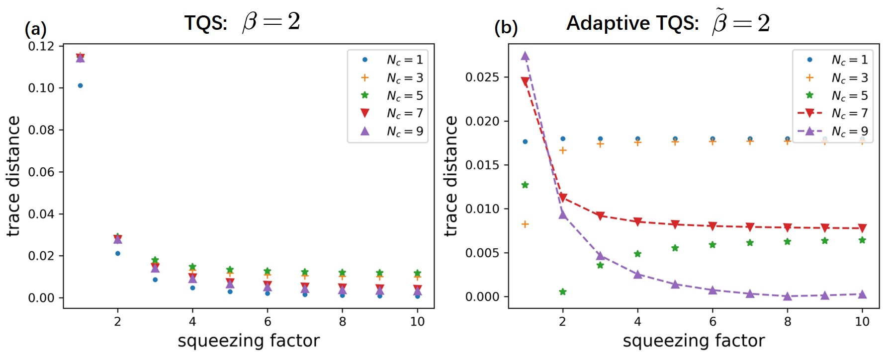
Figure 5: Effects on truncation of resource state in the Fock space for preparing thermal states of single qubit with two different approaches: $\beta$ ($\tilde{\beta}$) stands for results from TQS (adaptive TQS). Here, $N_{c}$ is the number of Fock basis of even-number photons, for instance, for $N_{c}=4$, $|0\rangle,|2\rangle,|4\rangle,|6\rangle$ are used.

Free energy. Accuracy simulation of free energy is key for thermal numeral simulation. Here, we present numeral results for free energies for the Kitaev ring for different $\lambda$ and $T$, as well as how it depends on the squeezing factor. As seen in Fig. 6, free energy can be simulated very accurately. Moreover, free energies at small squeezing factors are larger than exact results, which is consisted to theoretical analysis that says the quantum algorithm gives a bound from above for the free energy.

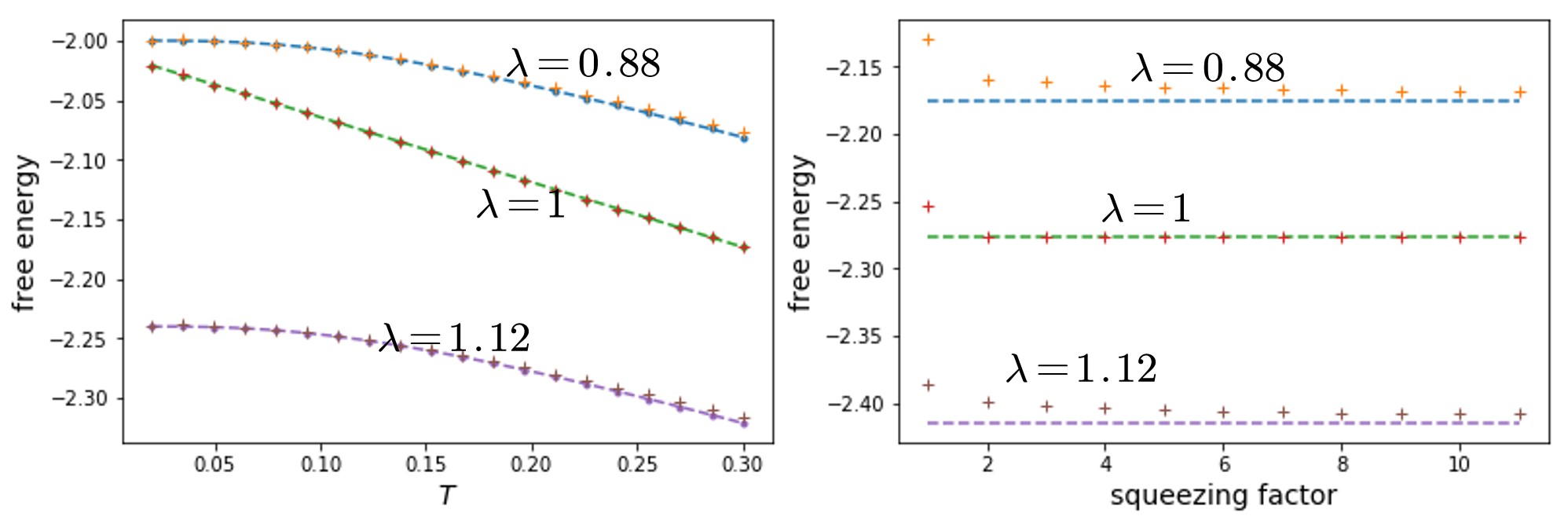
Figure 6: Free energies for the Kitaev ring at $L=2$. Dash lines correspond to exact results and markers are results from adaptive TQS. The left figure is obtained for a squeezing factor $s=10$, and the right figure is obtained at temperature $T=0.4$. All are calculated under a truncation of $N_{c}=35$.

Appendix E Decomposition of hybrid-variable quantum operators.

To simulate $e^{-iH\hat{p}t}$, we use a trotterization to decompose it into short time evolutions, evolving operators $e^{-i\delta\sigma^{i}_{z}\hat{p}}$, $e^{-i\delta\sigma^{i}_{x}\sigma^{i+1}_{x}\hat{p}}$, $e^{-i\delta\sigma^{1}_{y}P_{L}\sigma^{L}_{y}\hat{p}}$, and so on. We show that all those operators can be compiled into basic quantum gates of qubits and only one qubit-qumode hybrid quantum gate $e^{-i\delta\sigma_{x}\hat{p}}$, as illustrated in Fig. 7, which is similar to the technique in the textbook Nielsen and Chuang (2010). For convenience, we also denote $X=\sigma^{x},Y=\sigma^{y},Z=\sigma^{z}$. Here, we can use some basic single-qubit transformations,

$$HZH=X,~{}~{}~{}HXH=Z,~{}~{}~{}HYH=-Y,~{}~{}~{}SXS^{\dagger}=Y.$$ (22)

And those evolve CNOT gates,

$$CZ_{2}C=Z_{1}Z_{2},~{}~{}~{}CZ_{1}C=Z_{1},~{}~{}~{},CX_{1}C=X_{1}X_{2},~{}~{}~{}CX_{2}C=X_{2},$$ (23)

where we denote $C$ as CNOT gate with qubit 1 as control and qubit 2 as target. We remark $e^{-i\delta\sigma^{i}_{x}\sigma^{i+1}_{x}\hat{p}}$ can be seen as parity-dependence displacement operator, where the direction of displacement depends on the parity $\sigma^{i}_{x}\sigma^{i+1}_{x}$.

For the Kitaev ring, specifically evolutions of $\sigma_{1}^{y}P_{L}\sigma_{L}^{y}\hat{p}$ can be decomposed, following the method in Fig. (7), where we have shown the case $L=2,3$. For other $L$, one can use an identity,

$$e^{-i\delta\sigma_{1}^{y}\sigma_{2}^{z}...\sigma_{L}^{y}\hat{p}}=S_{1}H_{1}S_{L}H_{L}He^{-i\delta\sigma_{1}^{z}\sigma_{2}^{z}...\sigma_{L}^{z}\hat{p}}H_{1}H_{L}S_{1}^{\dagger}S_{L}^{\dagger},$$ (24)

where $e^{-i\delta\sigma_{1}^{z}\sigma_{2}^{z}...\sigma_{L}^{z}\hat{p}}$ can be constructed with the same fashion as $e^{-i\delta\sigma_{1}^{z}\sigma_{2}^{z}}$ and $e^{-i\delta\sigma_{1}^{z}\sigma_{2}^{z}\sigma_{3}^{z}}$.

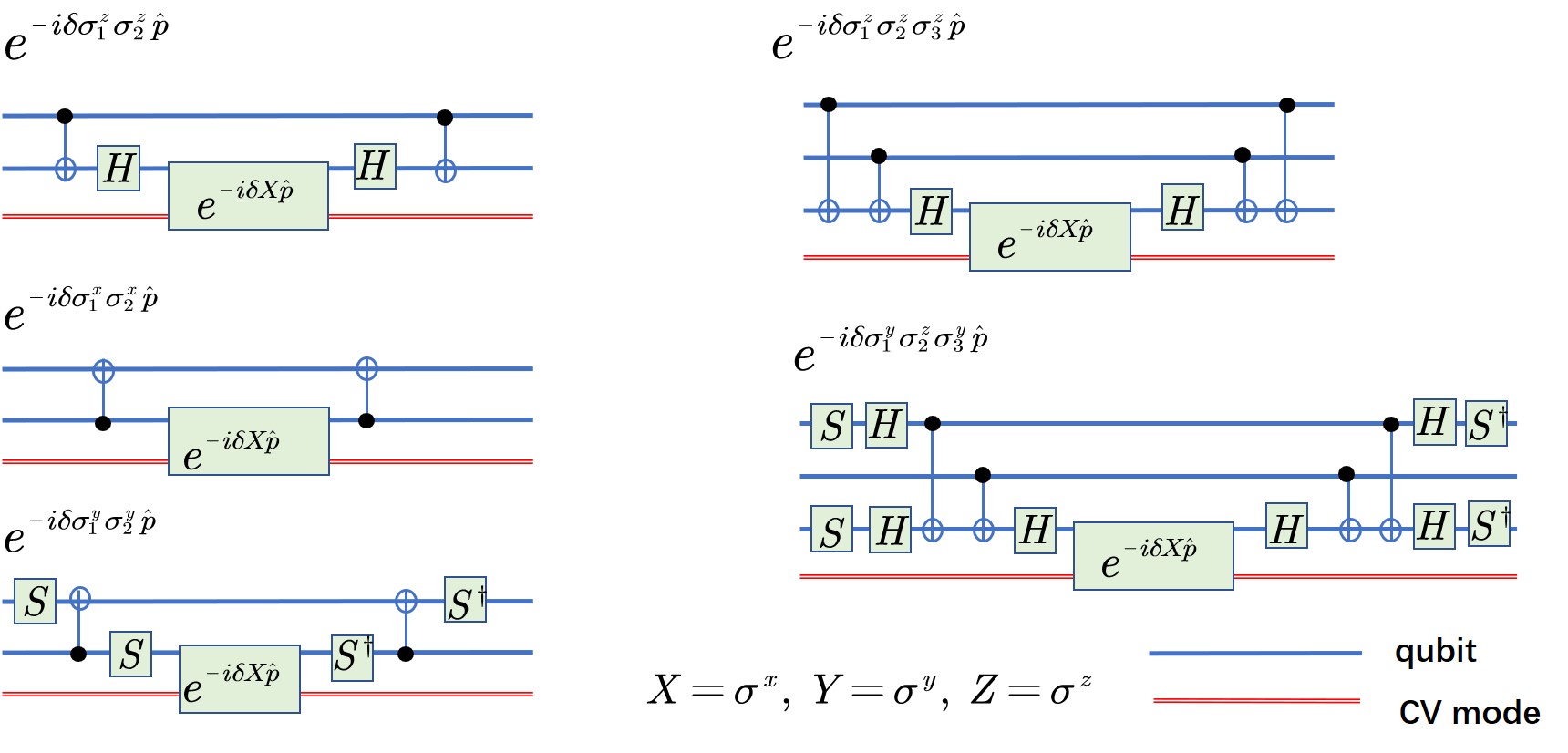
Figure 7: Decomposition of hybrid quantum gates with a series of CNOT and a qubit-qumode gate $e^{-i\delta\sigma_{x}\hat{p}}$.

Appendix F Requirement of squeezing factor

The task is to calculate the requirement of $s$ with the required accuracy $\epsilon$ for simulating quantum thermal state with the inverse temperature $\beta$. For this we use a relative accuracy $\epsilon$ of both the partition function and the quantum Gibbs distribution. It is expected that the former is less demanding for squeezing factor under relative accuracy $\epsilon$. In the following, we find that both may give the same dependence of the squeezing factor $s$ on $\epsilon$. We first consider TQS for $\beta$ using $|R(\beta)\rangle$, assuming that an arbitrary resource state can be prepared. Then, we consider adaptive TQS with an easy-to-prepare resource state.

A relative accuracy $\epsilon$ of the partition function is defined as

$$e(\beta,s):=\frac{|\tilde{\mathcal{Z}}(\beta,s)-\mathcal{Z}(\beta)|}{\mathcal{Z}(\beta)}\leq\epsilon.$$ (25)

Here $\tilde{\mathcal{Z}}(\beta,s)\propto\int_{E_{\text{0}}}^{E_{\text{1}}}a^{2}(E,\beta,s)D(E)dE$, where $D(E)$ is spectral density of the system. Note that $\tilde{\mathcal{Z}}(\beta,s)-\mathcal{Z}(\beta)$ can be approximated as

$$\int_{E_{\text{1}}}^{E_{\text{0}}}D(E)dE\int_{-\infty}^{\infty}dp\frac{2}{\pi}\frac{\beta}{\beta^{2}+4p^{2}}(e^{-\frac{p^{2}}{2s^{2}}}-1)e^{-iEp}$$

$$\times\int_{-\infty}^{\infty}dp\frac{2}{\pi}\frac{\beta}{\beta^{2}+4p^{2}}(e^{-\frac{p^{2}}{2s^{2}}}+1)e^{-iEp}$$

$$=-16\int_{E_{\text{0}}}^{E_{\text{1}}}dED(E)(e^{\frac{\beta^{2}}{8s^{2}}}-1)(e^{\frac{\beta^{2}}{8s^{2}}}+1)e^{-\beta E},$$ (26)

where in the third line we have applied Cauchy’s residue theorem in complex analysis, with an integral of $p$ in the half complex plane enclosing the pole $p=-i\beta/2$ (the other pole is not used since the integral must depend on $E$). We note that Eq. (F) is small than zero, which suggests that the quantum algorithm would give a bound from below for the partition function, and consequently a bound from above for the free energy.

For small $s/\beta$, using $e^{x}\approx 1+x$, then

$$e(\beta,s)\sim\frac{2\beta^{2}}{s^{2}}\frac{\int_{E_{\text{0}}}^{E_{\text{1}}}dED(E)e^{-\beta E}}{\int_{E_{\text{0}}}^{E_{\text{1}}}dED(E)e^{-\beta E}}=\frac{2\beta^{2}}{s^{2}}$$ (27)

It is interesting to note that the final expression is independent of the details of the spectral function. For TQS of $\beta$ using a resource state $|R(\beta)\rangle$, to achieve $e(\beta,s)\leq\epsilon$ at inverse temperature $\beta$, the required squeezing factor is $s\sim\beta\epsilon^{-\frac{1}{2}}$.

We now consider adaptive TQS at inverse temperature $\beta$ with a resource state $|R(\beta_{0})\rangle$. Eq. (F) then is,

$$\int_{E_{\text{1}}}^{E_{\text{0}}}D(E)dE\int_{-\infty}^{\infty}dp\frac{2}{\pi}\frac{\beta_{0}}{\beta_{0}^{2}+4p^{2}}(e^{-\frac{p^{2}}{2s^{2}}}-1)e^{-iEp\frac{\beta}{\beta_{0}}}$$ (28)

$$\times\int_{-\infty}^{\infty}dp\frac{2}{\pi}\frac{\beta_{0}}{\beta_{0}^{2}+4p^{2}}(e^{-\frac{p^{2}}{2s^{2}}}+1)e^{-iEp\frac{\beta}{\beta_{0}}}$$

$$=-16\int_{E_{\text{0}}}^{E_{\text{1}}}dED(E)(e^{\frac{\beta_{0}^{2}}{8s^{2}}}-1)(e^{\frac{\beta_{0}^{2}}{8s^{2}}}+1)e^{-\beta E}.$$

One can get $s\sim\epsilon^{-\frac{1}{2}}$, which is independent of $\beta$. This can explain why adaptive TQS is less demanding for squeezing. The cost, however, is that the complexity to construct the unitary evolution increases with a factor $\beta^{2}$.

For a relative error $\epsilon$ of the Gibbs distribution, it requires that

$$e(\beta,s):=\frac{|a^{2}(E,\beta,s)/\tilde{\mathcal{Z}}(\beta,s)-e^{-\beta E}/\mathcal{Z}(\beta,s)|}{e^{-\beta E}/\mathcal{Z}(\beta,s)}\leq\epsilon.$$

It can be verified that a scaling of $s\sim\beta\epsilon^{-\frac{1}{2}}$ ($s\sim\epsilon^{-\frac{1}{2}}$) can satisfy this relative error for TQS (adaptive TQS). In fact, following the same technique of relative error of partition function, the same scaling of squeezing factor with $\beta$ and $\epsilon$ can be obtained.