Non-Markovian quantum dynamics: Extended correlated projection superoperators

Abstract

The correlated projection superoperator techniques provide a better understanding about how correlations lead to strong non-Markovian effects in open quantum systems. Their superoperators are independent of initial state, which may not be suitable for some cases. To improve this, we develop a new approach, that is extending the composite system before use the correlated projection superoperator techniques. Such approach allows choosing different superoperators for different initial states. We apply these techniques to a simple model to illustrate the general approach. The numerical simulations of the full Schrödinger equation of the model reveal the power and efficiency of the method.

I Introduction

In both experimental and theoretical research, people are often interested in only parts of objects, but there are always interactions between the parts of the whole. Hence, the open system is common and important. A detailed review of open quantum systems can be found in BP02 ; VA17 . The dynamics of system usually satisfy the Markov approximation, which makes such processes history independent. In quantum dynamics, the evolution of such systems is described by the well-known Lindblad equation. As our ability to observe and control quantum system increases, non-Markovian behavior is becoming increasingly important.

The Nakajima-Zwanzig (NZ) equation and time-convolutionless (TCL) equation are powerful tools to analyze the open quantum systems. With the Markov approximation, they can provide a Lindblad master equation. Without this approximation, the equations can be used to describe non-Markovian behavior. Both of them are widely used in the research of open systems. To solve the equations, one often needs perturbation expansion with respect to the system-environment coupling. Approximations of the same order via these two methods can have very different physical meanings and ranges of applicability. In general, the TCL techniques are better R03 .

The NZ and TCL equations often use the projection-operator method to derive the dynamic equation of the system. The original projection-operator method uses a projection superoperator (PS). The superoperator maps the total density matrix to a tensor product state, which is called the relevant part. Total density matrix minus its relevant part represents the irrelevant part. The tensor product state omits any correlations between system and environment. However, the correlations play a key role in non-Markovian behavior of open systems. This makes the PS method not suitable for the research of non-Markovian behavior.

To study open quantum systems with highly non-Markovian behavior, the correlated projection superoperator (CPS) techniques were proposed BGM06 ; B07 . The CPS techniques map the total density matrix to a quantum-classical state. This enables the relevant part to contain classical correlations and some quantum correlations, which may lead highly non-Markovian behavior. However, the quantum discord and entanglement between system and environment is still lacking in the relevant part. A detailed review of correlations can be found in MPSVW10 ; S15 . Comparing with PS techniques, CPS techniques generally provide a better understanding about the influence of the correlations between system and environment. It also yields accurate results already in the lowest order of the perturbation expansion BGM06 ; FB07 . However, the accuracy of this approach relies on the choice of projection superoperators. An inappropriate superoperator can lead to disastrous results.

The CPS techniques are very general. To develop it, we first extend the environment space with an ancillary system. After that, we use CPS techniques in the enlarged space to get the evolution of relevant part. Although the relevant part here is still a quantum-classical state in the enlarged space, it allows the quantum discord between system and environment. Finally, the evolution of the system is obtained by tracing over environment and ancillary system. We call it extended correlated projection superoperator (ECPS) techniques. Compared with CPS, the ECPS provides more relevant variables. Hence, the relevant part permits more correlations. Besides that, the method may yield more accurate results.

The basic idea underlying ECPS method is that one can separate the initial state into several pure states, and use different CPS to each pure state. This allows using the best CPS for each state; hence it probably yields more accurate results. If all the state share the same superoperator, the ECPS techniques will go back to the CPS techniques, which means the CPS techniques are good enough. The interaction of such systems often satisfies some conservation law. Such as conservation of energy BGM06 , or conservation of angular momentum FB07 . The conservation law often leads to classical correlations in those conserved quantities. If such conservation law is absent, as we will present in Sec. III, then only the ECPS techniques can ensure the accuracy of the results. Moreover, this approach allows the treatment of initial states with non-vanished quantum discord by means of a homogeneous NZ or TCL equation.

A homogeneous equation is easier. However, the form of superoperator is mainly determined by interaction and steady state. A homogeneous master equation given by PS method is only applicable for some special initial states. For other states, even if the irrelevant part can be vanished under some special superoperators. Their solution may diverge in the limit $t\to\infty$. In such cases, the homogeneous master equation given by the standard approach fails in any finite order of the coupling strength. With ECPS method, the choice of projection superoperators is more flexible. Therefore, it’s easier to obtain a convergence results under the homogeneous master equation.

We organize the paper as follows. In Sec. II we briefly review the standard projection-operator method and the CPS techniques. We also review how to formulate the NZ equation and the TCL equation. After that, we introduce the ECPS techniques and provide a rough criterion to determine whether it needed. With the ECPS techniques, one can choose different projection superoperators for different initial states, which is totally different from the CPS method. We also briefly discuss how to choose an appropriate projection superoperator. In Sec. III we apply the ECPS techniques to a system-reservoir model. We discuss when the best projection superoperator is dependent on initial state. Then, we show that any single projection superoperator can’t ensure accurate results for all initial states in some cases. This implies that the ECPS techniques are necessary in these cases. After that, we explore the origin of the failure of the homogeneous master equation. We show the ECPS techniques can provide a homogeneous master equation without divergence problems for more initial states. In Sec. IV we conclude the paper and briefly discuss possible future developments of ECPS techniques.

II PROJECTION OPERATOR TECHNIQUES

We consider an open quantum system $A$ is coupled with an environment $B$. Their Hilbert space of states are $\mathcal{H}_{A}$ and $\mathcal{H}_{B}$ respectively. The Hilbert space of states of the composite system is $\mathcal{H}_{A}\otimes\mathcal{H}_{B}$. The dynamics of the total density matrix $\rho_{AB}$ of the composite system is governed by some Hamiltonian of the form $H=H_{0}+\alpha H_{I}$, where $H_{0}=H_{A}+H_{B}$ generates the free time evolution of the system and of the environment. $H_{I}$ describes the system-environment coupling.

II.1 The projection-operator method

The PS techniques project the total density matrix of the composite system onto a tensor product state

$$\mathcal{P}\rho_{AB}\equiv(\text{Tr}_{B}\rho_{AB})\otimes\rho_{B}^{0},$$ (1)

where environment reference state $\rho_{B}^{0}$ is fixed in time. Since $\mathcal{P}^{2}=\mathcal{P}$, the superoperator $\mathcal{P}$ is called projection superoperator. The irrelevant part is given by the complementary map $\mathcal{Q}=I-\mathcal{P}$, where $I$ denotes the identity map. Obviously, the relevant part contains all the local information of the system $\text{Tr}_{B}\mathcal{P}\rho_{AB}=\rho_{A}$. And being a tensor product state, the relevant part can’t contain any system-environment correlation information.

The CPS techniques project the total density matrix onto a quantum-classical state

$$\mathcal{P}\rho_{AB}\equiv\sum_{\alpha}\text{Tr}_{B}(\Pi_{\alpha}^{B}\rho_{AB})\otimes\rho_{\alpha}^{B},$$ (2)

where different $\alpha$ denotes different subspace $\mathcal{H}_{\alpha}$ of environment. They’re orthogonal $\Pi_{\alpha}\Pi_{\beta}=\delta_{\alpha\beta}\Pi_{\beta}$ and complete $\sum_{\alpha}\Pi_{\alpha}=I^{B}$. $\Pi_{\alpha}^{B}$ is the identity matrix of $\mathcal{H}_{\alpha}$. $\rho_{\alpha}^{B}$ is the reference state of $\mathcal{H}_{\alpha}$. If we take all the subspace $\mathcal{H}_{\alpha}$ as one dimension, then all reference state must be a projection operator $\rho_{\alpha}^{B}=\Pi_{\alpha}^{B}$. In such cases, the CPS becomes

$$\mathcal{P}\rho_{AB}\equiv\sum_{i}\text{Tr}_{B}(\Pi_{i}^{B}\rho_{AB})\otimes\Pi_{i}^{B}.$$ (3)

The collection of projection operators $\{\Pi_{j}^{B}|j\}$ determine the projection superoperator, which directly affect the accuracy of the lower order master equation. We shall discuss it in detail in the section II.6. The definition of Eq. 2 and Eq. 3 is equivalent indeed: One can always diagonalize $\rho_{\alpha}^{B}$ and redefine the basis of $\mathcal{H}_{\alpha}$ to get Eq. 3 from Eq. 2.

From the definition, $\text{Tr}_{B}\mathcal{P}\rho_{AB}=\rho_{A}$ is satisfied in CPS. Hence, its relevant part also contains all the local information of the system. Besides that, since its relevant part is quantum-classical state, it can contain some system-environment correlation information.

The relevant part provided by the CPS techniques contains more relevant variables, which make its dynamic equation more complex. Besides that, to determine the initial relevant part in CPS techniques, one may need more information about the environment.

II.2 Nakajima-Zwanzig equation

In the interaction picture with respect to $H_{0}$, the von Neumann equation of the composite system can be written as

$$\frac{d}{dt}\rho_{AB}(t)=-i[\alpha H_{I}(t),\rho_{AB}(t)]\equiv\alpha\mathcal{L}(t)\rho_{AB}(t),$$ (4)

where $H_{I}(t)=e^{iH_{0}t}H_{I}e^{-iH_{0}t}$ is the Hamiltonian in the interaction picture and $\mathcal{L}(t)$ denotes the corresponding Liouville superoperator. It’s usually assumed that the relations

$$\mathcal{P}\mathcal{L}(t_{1})\mathcal{L}(t_{2})\dots\mathcal{L}(t_{2n+1})\mathcal{P}=0$$ (5)

hold for any natural number $n$. Based on the von Neumann equation, one can derive an exact dynamical equation of relevant part BP02

$$\frac{d}{dt}\mathcal{P}\rho_{AB}(t)=\int_{0}^{t}dt_{1}\mathcal{K}(t,t_{1})\mathcal{P}\rho_{AB}(t_{1})$$

$$+\alpha\mathcal{P}\mathcal{L}(t)\mathcal{G}(t,0)\mathcal{Q}\rho_{AB}(0),$$ (6)

where superoperator

$$\mathcal{K}(t,t_{1})=\alpha^{2}\mathcal{P}\mathcal{L}(t)\mathcal{G}(t,t_{1})\mathcal{Q}\mathcal{L}(t_{1})\mathcal{P}$$ (7)

is called the memory kernel or the self-energy. $\mathcal{G}(t,t_{1})=\mathcal{T}\exp[\alpha\int_{0}^{t}dt_{2}\mathcal{Q}\mathcal{L}(t_{2})]$ is the propagator, where $\mathcal{T}$ denotes chronological time ordering. section II.2 is called the NZ equation. The inhomogeneous term $\mathcal{P}\mathcal{L}(t)\mathcal{G}(t,0)\mathcal{Q}\rho_{AB}(0)$ depends on the initial conditions at time $t=0$. It vanishes if the irrelevant part vanishes at initial time. In PS techniques, if the initial state of the composite system is a tensor product state, one can choose the reference state $\rho_{B}^{0}=\rho_{B}(0)$ to make $\mathcal{Q}\rho_{AB}(0)=0$. In CPS techniques, if the initial state is quantum-classical state, one can always let $\mathcal{Q}\rho_{AB}(0)=0$ by choosing an appropriate projection superoperator. From this perspective, a benefit of CPS method is that one can obtain a homogeneous master equation for relevant part, even the initial state contains some correlations between system and environment.

Under the hypothesis (5), when the relevant part at initial time vanishes, the lowest-order contribution is given by the second order

$$\frac{d}{dt}\mathcal{P}\rho_{AB}(t)=\alpha^{2}\int_{0}^{t}dt_{1}\mathcal{P}\mathcal{L}(t)\mathcal{L}(t_{1})\rho_{AB}(t_{1}).$$ (8)

II.3 Time-convolutionless master equation

TCL master equation is an alternative way to deriving an exact master equation. It is a time-local equation of motion and doesn’t depend on the full history of the system. The equation can be written as

$$\frac{d}{dt}\mathcal{P}\rho_{AB}(t)=\mathcal{K}(t)\mathcal{P}\rho_{AB}(t)+\mathcal{I}(t)\mathcal{Q}\rho_{AB}(0).$$ (9)

$\mathcal{K}(t)$ is called the TCL generator, which can be expanded in terms of $H_{I}$. The expansion can be obtained from ordered cumulants BP02 . By hypothesis (5), all odd-order contributions vanish. The second-order contribution reads

$$\mathcal{K}_{2}(t)=\alpha^{2}\int_{0}^{t}dt_{1}\mathcal{P}\mathcal{L}(t)\mathcal{L}(t_{1})\mathcal{P}.$$ (10)

Combining Eqs. 9 and 10, if the inhomogeneous term vanishes, one obtains

$$\frac{d}{dt}\mathcal{P}\rho_{AB}(t)=\alpha^{2}\int_{0}^{t}dt_{1}\mathcal{P}\mathcal{L}(t)\mathcal{L}(t_{1})\mathcal{P}\rho_{AB}(t).$$ (11)

This is a second-order TCL master equation for relevant part. The equations of motion provided by NZ and TCL techniques are different in any finite order. But their exact solution should be the same. Hence, their accuracy is of the same order. In the following section, we will use TCL approach.

II.4 Extended correlated projection superoperators

The CPS techniques use the most general linear projection superoperators that keeps all the local information of the system. However, since it uses a single superoperator for all the initial states. One can not select the projection superoperators according to the initial state. Moreover, its relevant part must lose some correlation, for instance, quantum discord and entanglement. Here we propose a method that allows choosing superoperators for different initial states. One incidental benefit is that the relevant part can contain quantum discord between system and environment now. The basic idea underlying our approach is the following. The initial state of the composite system can always be separated into several states $\rho^{i}_{AB}$. Its evolution comes directly from the evolution of these separated states $\rho_{AB}(t)=\sum_{i}P^{i}\rho^{i}_{AB}(t)$. If we use CPS separately, then choosing superoperators for different initial states is applicable. Moreover, since using different superoperators are permitted, the sum of those relevant part allows quantum discord, even the relevant part for each of them $\mathcal{P}^{i}\rho^{i}_{AB}$ doesn’t contain quantum discord.

The steps of the ECPS methods are as follows:

• Extend the environment with an ancillary system and map the initial state $\rho_{AB}=\sum_{i}P^{i}\rho^{i}_{AB}$ to a quantum-classical state $\rho_{ABC}=\sum_{i}P^{i}\rho^{i}_{AB}\otimes\Pi^{i}_{C}$.

• Use CPS techniques in the extended space as $\mathcal{P}\rho_{ABC}=\sum_{i,j}\text{Tr}_{BC}(\Pi_{i,j}^{B}\otimes\Pi_{i}^{C}\rho_{ABC})\otimes\Pi_{i,j}^{B}\otimes\Pi_{i}^{C}$, where the collection of projection operators $\{\Pi_{i,j}^{B}|j\}$ with different index $i$ provides a complete set $\sum_{j}\Pi_{i,j}^{B}=I^{B}$.

• Solve the master equation to get the evolution of relevant part $\mathcal{P}\rho_{ABC}(t)$.

• The evolution of the system $\rho_{A}(t)$ can be obtained from the relevant part $\mathcal{P}\rho_{ABC}(t)$ by partial tracing in the environment and ancillary system.

In this procedure, the relevant part of each state is $\mathcal{P}^{i}\rho^{i}_{AB}=\text{Tr}_{C}(\Pi_{i}^{C}\mathcal{P}\rho_{ABC})$. The ancillary space denotes that different states can use different CPS, i.e., $\{\Pi_{i,j}^{B}|j\}$ can be different for different $i$. Therefore, though $\mathcal{P}\rho_{ABC}(t)$ is still a quantum-classical sate, $\text{Tr}_{C}\mathcal{P}\rho_{ABC}(t)$ allows quantum discord between system and environment.

One advantage of ECPS method is that its homogeneous master equation has a wider range of applications, such as cases that the initial state contains quantum discord between system and environment. A pure state is quantum correlated if and only if the state is entangled S15 . If the system isn’t entangled with environment initially, i.e., the initial state is separable, one can separate it into several pure states. Since the composite system is isolated, those states remain pure during the evolution. Hence, the pure state $\rho^{i}_{AB}$ won’t contain quantum discord. Correspondingly, the master equation of each pure state $\rho^{i}_{AB}$ can be homogeneous. And the master equation of relevant part $\mathcal{P}\rho_{ABC}$ can still be homogeneous, even the initial state $\rho_{AB}(0)$ does contain quantum discord.

Besides that, for pure state $\rho^{i}_{AB}$, its distance from separable states is the same as its distance from classical correlated states

$$\|\rho^{i}_{AB}-\mathcal{S}^{i}_{A:B}\|\equiv\min_{\sigma\in\mathcal{S}_{A:B}}\|\rho_{AB}^{i}-\sigma\|=\min_{\sigma\in\mathcal{C}_{A:B}}\|\rho_{AB}^{i}-\sigma\|,$$ (12)

where $\mathcal{C}_{A:B}$ is the set of classical correlated states and $\mathcal{S}_{A:B}$ is the set of separable states. According to Eq. 12, the irrelevant part in the ECPS techniques can be directly related to entanglement. This means that even the irrelevant part is non-trivial, the inhomogeneous term can always be upper bounded by the entanglement. An intriguing fact is that a general monogamy correlation measure beyond entanglement doesn’t exist SAPB12 . Hence, it’s impossible to find a similar result in the CPS techniques.

The shortage of ECPS method is that the dynamical equation is more complicated. And the entanglement between the system and the environment is still lacking in its relevant part. But, as we will explain below, include entanglement in relevant part may be unnecessary:

• If the relevant part contains all the local information of the system and all the system-environment correlation information, then it already contains all system-related information in the composite system. Such relevant part is equivalent to the total density matrix of the composite system. It can be treated as a closed system and its evolution is unitary.

• The entanglement is monogamy. In many cases, the system-environment state is almost indistinguishable from the separable state due to quantum de Finetti’s theorem ZCZW15 .

• Though the relevant part of ECPS can’t contain entanglement, one can still take it into account with irrelevant part. The monogamy properties of entanglement may be helpful to simplify the inhomogeneous term.

The PS techniques, CPS techniques and ECPS techniques project the total density matrix onto tensor product states, quantum-classical states, separable states respectively. These approaches together with unitary evolution of closed systems compose a complete picture about the dynamics of the system, from the perspective of correlation. Each of them has its applications. The ECPS techniques can improve the accuracy of the lower-order equation, but also increase the complexity of equation. And It needs more information about the environment.

The dynamics of the open system is uniquely determined by the dynamical variables

$$\rho_{i,j}(t)\equiv\text{Tr}_{BC}(\Pi_{i,j}^{B}\otimes\Pi_{i}^{C}\rho_{ABC}(t)),$$ (13)

from which the density matrix of the system reads

$$\rho_{s}(t)=\sum_{i,j}\rho_{i,j}(t).$$ (14)

The normalization condition is obviously satisfied

$$\text{Tr}_{s}\rho_{s}(t)=\sum_{i,j}\text{Tr}_{ABC}(\Pi_{i,j}^{B}\otimes\Pi_{i}^{C}\rho_{ABC}(t))=1.$$ (15)

Suppose initial relevant part is vanished, from NZ equation section II.2, the evolution equation of the dynamical variables becomes

$$\frac{d}{dt}\rho_{i,j}(t)=\sum_{k}\int_{0}^{t}dt_{1}\mathcal{K}_{jk}^{i}(t,t_{1})\rho_{i,k}(t_{1}),$$ (16)

where the superoperator

$$\mathcal{K}_{jk}^{i}(t,t_{1})\mathcal{O}_{A}\equiv\text{Tr}_{BC}\{\Pi_{i,j}^{B}\otimes\Pi_{i}^{C}\mathcal{K}(t,t_{1})(\mathcal{O}_{A}\otimes\Pi_{i,k}^{B}\otimes\Pi_{i}^{C})\}.$$ (17)

From TCL equation Eq. 11, we have

$$\frac{d}{dt}\rho_{i,j}(t)=\sum_{k}\mathcal{K}_{jk}^{i}(t)\rho_{i,k}(t),$$ (18)

where the TCL generator is defined as

$$\mathcal{K}_{jk}^{i}(t)\mathcal{O}_{A}\equiv\text{Tr}_{BC}\{\Pi_{i,j}^{B}\otimes\Pi_{i}^{C}\mathcal{K}(t)(\mathcal{O}_{A}\otimes\Pi_{i,k}^{B}\otimes\Pi_{i}^{C})\}.$$ (19)

Eq. 16 can be written as

$$\frac{d}{dt}\mathcal{P}^{i}\rho_{i}(t)=\mathcal{K}^{i}(t)\mathcal{P}^{i}\rho_{i}(t),$$ (20)

where $\mathcal{P}^{i}\rho_{AB}=\sum_{j}\text{Tr}_{BC}(\Pi_{i,j}^{B}\rho_{AB})\otimes\Pi_{i,j}^{B}$ and

$$\rho_{i}(t)=\text{Tr}_{C}(\Pi_{i}^{C}\rho_{ABC}(t))=P^{i}\rho^{i}_{AB}.$$ (21)

Comparing Eq. 9 with Eq. 20, it’s easy to find that the ECPS method is just applying different CPS $\mathcal{P}^{i}$ to each pure state $\rho_{i}$. Similar to Eq. 11, the second-order TCL equation in ECPS techniques can be written as

$$\frac{d}{dt}\mathcal{P}^{i}\rho_{i}(t)=\alpha^{2}\int_{0}^{t}dt_{1}\mathcal{P}^{i}\mathcal{L}(t)\mathcal{L}(t_{1})\mathcal{P}^{i}\rho_{i}(t).$$ (22)

II.5 Whether the ECPS techniques are necessary

A collection of projection operators can be parameterized as

$$\Pi_{i,j}^{B}=U(\bm{\theta}^{i})|j\rangle\langle j|U^{\dagger}(\bm{\theta}^{i}).$$ (23)

The TCL equation Eq. 9 is exact and its solution should be independent of the parameters $\bm{\theta}$. However, the second-order TCL generator $\mathcal{K}^{i}_{2}(\bm{\theta}^{i},t)$ is true depends on $\bm{\theta}$, so does its approximate solution. In principle, the difference $\mathcal{K}^{i}(t)-\mathcal{K}^{i}_{2}(\bm{\theta}^{i},t)$ can tell whether a projection superoperator is appropriate. However, it’s hard to obtain $\mathcal{K}^{i}(t)$, which needs infinity order of expansion.

An alternative way to judge a projection superoperator is from the unitary evolution of the composite system

$$\rho(t)=\mathcal{T}\exp[\alpha\int_{0}^{t}ds\mathcal{L}(s)]\rho(0)=(1+\alpha\int_{0}^{t}dt_{1}\mathcal{L}(t_{1})$$

$$+\alpha^{2}\int_{0}^{t}dt_{1}\int_{0}^{t_{1}}dt_{2}\mathcal{L}(t_{1})\mathcal{L}(t_{2})+\dots)\rho(0).$$ (24)

Differentiating this equation with respect to time, we obtain

$$\partial_{t}\rho(t)=(\alpha\mathcal{L}(t)+\alpha^{2}\int_{0}^{t}dt_{2}\mathcal{L}(t)\mathcal{L}(t_{2})+\dots)\rho(0).$$ (25)

The initial state of the composite system can be expressed as $\rho(0)=\mathcal{T}_{\to}\exp[-\alpha\int_{0}^{t}ds\mathcal{L}(s)]\rho(t)$, where $\mathcal{T}_{\to}$ denotes the antichronological time-ordering operator. Substituting it into Eq. 25, we obtain a time-local equation

$$\frac{d}{dt}\rho(t)=\mathcal{K}_{\text{tot}}(t)\rho(t),$$ (26)

where superoperator $\mathcal{K}_{\text{tot}}$ is independent of projection superoperator. The error produced by expansion should be determined by the expansion order $\|\mathcal{K}^{2}_{\text{tot}}(t)-\mathcal{K}_{\text{tot}}(t)\|\sim O(\alpha^{3})$. Results from the second order $\mathcal{K}^{2}_{\text{tot}}(t)$ should be pretty accurate if the perturbation theory is applicable in the composite system. Hence, it may be appropriate to use the difference of superoperators

$$\mathcal{P}_{\theta}\mathcal{K}^{2}_{\text{tot}}(t)-\mathcal{K}_{2}(\bm{\theta},t)$$ (27)

to determine whether a projection superoperator is suitable. The distinguishability of superoperator can be characterized by norm K97

$$\|\Phi_{0}-\Phi_{1}\|_{1}\equiv\max\{\|\Phi_{0}(|\psi\rangle\langle\psi|)-\Phi_{1}(|\psi\rangle\langle\psi|)\|_{1}\},$$ (28)

where $\||\psi\rangle\|=1$. A more precise norm K97 is

$$\|\Phi_{0}-\Phi_{1}\|_{\lozenge}\equiv\|(\Phi_{0}-\Phi_{1})\otimes I\|_{1}.$$ (29)

If the norm $\|\mathcal{P}_{\theta}\mathcal{K}^{2}_{\text{tot}}(t)-\mathcal{K}_{2}(\bm{\theta},t)\mathcal{P}_{\theta}\|_{\lozenge}$ can be zero with parameters $\bm{\theta}$, then the collection of projection operators $\{\Pi^{B}(\bm{\theta})\}$ is sufficiently accurate for all initial state. In such cases, the CPS techniques are good enough. Otherwise, the best projection superoperator may depend on the initial state, and one may need ECPS techniques to improve the accuracy.

The norm in Eq. 29 is based on the maximum distance of all states. It determines whether the ECPS techniques are necessary, but can’t tell which projection superoperator is the best for a specific state. The norm $\|(\mathcal{P}_{\theta}\mathcal{K}^{2}_{\text{tot}}(t)-\mathcal{K}_{2}(\bm{\theta},t)\mathcal{P}_{\theta})\rho\|_{1}$ can reflect the accuracy for a specific state. But, since the state of the composite system can change during the evolution, such norm can’t figure out which projection superoperator is better for the whole process of evolution. The exact relationship between the best projection superoperator and the initial states is beyond the scope of this paper. We leave this as an open question.

Finding an exact relationship is difficult, but seeking candidates for some special cases is easy. We will discuss this in the following section.

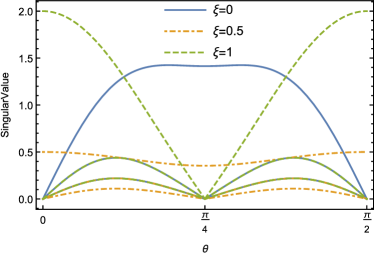
Figure 1: The singular values of Choi matrix of Eq. 48 under different projection superoperators and different interactions. For each $\xi$, there are at most three nontrivial singular values. Parameters: $\lambda=\alpha^{2}\gamma N=1$.

II.6 The appropriate projection superoperator

In CPS techniques, one can construct the projection superoperators with the help of the conserved quantity of interaction $H_{I}$ FB07 . Suppose that $C$ is a such conserved quantity, one can choose a collection of projection operators by the eigenstates of $C$

$$\{\Pi_{i}^{B}:C|i\rangle=\lambda_{i}|i\rangle\}.$$ (30)

Choosing an appropriate projection superoperator for each state $\rho^{i}_{AB}$ is also critical in ECPS techniques. Within the scope of ECPS method, the best projection superoperator should depend on initial state. And there should be no conserved quantity as that used in the CPS techniques. If the interaction $H_{I}$ can be separated into several terms $H_{I}=\sum_{i}\alpha_{i}H_{I}^{i}$, and each term $H_{I}^{i}$ has a conserved quantity $C_{i}$, then one can construct the best projection superoperator with the eigenstates of one of the conserved quantities $C_{k}$

$$\{\Pi_{i,j}^{B}:C_{k}|i,j\rangle=\lambda_{j}^{k}|i,j\rangle\}.$$ (31)

Which $C_{k}$ to use, from the interaction and initial state of the model, is still a problem. In the next section, we will briefly discuss this issue with a system-reservoir model. A systematic analysis is beyond the scope of this paper.

III Application

III.1 The model

To illustrate the general considerations of the previous sections, we apply the ECPS techniques to a two-state system $S$. The model was adapted from BGM06 . The two states of the system are degenerate. The system is coupled to an environment $E$, which consists of $N$ equidistant energy levels in an energy bands of width $\delta\epsilon$, and each energy level is doubly degenerate. The total Hamiltonian of the model in the Schrödinger picture is $H=H_{0}+\alpha(V_{1}+V_{2})$, where

$$H_{0}=\sum_{n=1}^{N}\sum_{i=1,2}\frac{\delta\epsilon}{N}n|n,i\rangle\langle n,i|,$$ (32)

and

$$V_{1}=(1-\xi)\sum_{n_{1},n_{2}}c(n_{1},n_{2})\sigma_{+}|n_{1},1\rangle\langle n_{2},2|+\text{H. c},$$

$$V_{2}=\xi\sum_{n_{1},n_{2}}c^{\prime}(n_{1},n_{2})\sigma_{\to}|n_{1},+\rangle\langle n_{2},-|+\text{H. c}.$$ (33)

Here $\sigma_{+}=(\sigma_{x}-i\sigma_{y})/2$ and $\sigma_{\to}=(\sigma_{y}-i\sigma_{z})/2$. $\{\sigma_{i}|i=x,y,z\}$ is the standard Pauli matrices. The environment state $|n_{1},\pm\rangle\equiv(|n_{1},1\rangle\pm|n_{1},2\rangle)/\sqrt{2}$. The coupling constant $c(n_{1},n_{2})$ and $c^{\prime}(n_{1},n_{2})$ are independent and identically distributed complex Gaussian random variables satisfying

$$\langle c(n_{1},n_{2})\rangle=\langle c^{\prime}(n_{1},n_{2})\rangle=0,$$ (34)

$$\langle c(n_{1},n_{2})c(n_{3},n_{4})\rangle=\langle c^{\prime}(n_{1},n_{2})c^{\prime}(n_{3},n_{4})\rangle=0,$$

$$\langle c(n_{1},n_{2})c^{*}(n_{3},n_{4})\rangle=\langle c^{\prime}(n_{1},n_{2})c^{\prime*}(n_{3},n_{4})\rangle$$

$$=\delta_{n_{1},n_{3}}\delta_{n_{2},n_{4}},$$

$$\langle c(n_{1},n_{2})c^{\prime}(n_{3},n_{4})\rangle=\langle c(n_{1},n_{2})c^{\prime*}(n_{3},n_{4})\rangle=0.$$

It’s easy to check that interaction operator $V_{1}$ and $V_{2}$ don’t commute with each other $[V_{1},V_{2}]\neq 0$. But their commutator is vanished in average of those random variable, i.e., $\langle[V_{1},V_{2}]\rangle=0$.

In the interaction picture, the Hamiltonian of von Neumann equation (4) is $H_{I}(t)=V_{1}(t)+V_{2}(t)$, where

$$V_{1}(t)=(1-\xi)(\sigma_{+}B(t)+\sigma_{-}B^{\dagger}(t));$$

$$V_{2}(t)=\xi(\sigma_{\to}B^{\prime}(t)+\sigma_{\leftarrow}B^{\prime\dagger}(t))$$ (35)

and

$$B(t)=\sum_{n_{1},n_{2}}c(n_{1},n_{2})e^{-i\omega(n_{1},n_{2})t}|n_{1},1\rangle\langle n_{2},2|,$$

$$B^{\prime}(t)=\sum_{n_{1},n_{2}}c^{\prime}(n_{1},n_{2})e^{-i\omega(n_{1},n_{2})t}|n_{1},+\rangle\langle n_{2},-|.$$ (36)

The energy difference $\omega(n_{1},n_{2})=\delta\epsilon(n_{2}-n_{1})/N$.

When $\xi=0$, the CPS techniques is enough, just as its predecessor. Suppose an environment operator $\mathcal{O}$ satisfies

$$\mathcal{O}|n_{1},1\rangle=-|n_{1},1\rangle;\mathcal{O}|n_{1},2\rangle=|n_{1},2\rangle.$$ (37)

Then $\mathcal{O}+\sigma_{z}$ is a conserved quantity of Hamiltonian $H$. Following the principle mentioned in section II.6, the best projection superoperator can be constructed with $\Pi^{1,2}$, where $\Pi^{i}=\sum_{n}|n,i\rangle\langle n,i|$. Such superoperator is the same as that used in BGM06 . Similar, when $\xi=1$, the best projection superoperator should be constructed with $\Pi^{+,-}$. When $0<\xi<1$, there is no such conserved quantity anymore. As explained in section II.6, we need ECPS techniques in such cases. The best projection superoperator should be constructed with $\Pi^{1,2}$ or $\Pi^{+,-}$. It depends on the specific initial state to decide which one is better.

III.2 TCL master equation from ECPS techniques

Suppose the projection superoperator in Eq. 20 is

$$\mathcal{P}_{\theta}\rho_{AB}=\sum_{i=1,2`}\text{Tr}_{B}(\Pi^{i}_{\theta}\rho_{AB})\otimes\Pi^{i}_{\theta}/N,$$ (38)

where $\Pi^{i}_{\theta}=\sum_{n}|n,i,\theta\rangle\langle n,i,\theta|$ and

$$\left(\begin{array}[]{c}|n,1,\theta\rangle\\ |n,2,\theta\rangle\\ \end{array}\right)=\left(\begin{array}[]{cc}\cos\theta&\sin\theta\\ \sin\theta&\cos\theta\\ \end{array}\right)\left(\begin{array}[]{c}|n,1\rangle\\ |n,2\rangle\\ \end{array}\right).$$ (39)

With $\theta=0$, $\Pi^{i}_{\theta}$ reads $\Pi^{1,2}$. With $\theta=\pi/4$, it gives $\Pi^{+,-}$. According to Eq. 22, the second-order TCL generator can be expressed as

$$\mathcal{K}^{i}(t)=\alpha^{2}\int_{0}^{t}dt_{1}\mathcal{P}_{\theta}\langle\mathcal{L}(t)\mathcal{L}(t_{1})\rangle\mathcal{P}_{\theta}.$$ (40)

According to Eq. 34, the random variables are independent of each other, so the total generator can be obtained by just adding two generators of corresponding interaction

$$\mathcal{K}^{i}(t)=\mathcal{K}^{i}_{1}(t)+\mathcal{K}^{i}_{2}(t),$$ (41)

where $\mathcal{K}^{i}_{1,2}(t)$ are the second-order TCL generator of $V_{1,2}$ respectively. Based on calculations in appendix A, all terms in the generator $\mathcal{K}^{i}_{1,2}(t)$ share the same time-dependent part $h(\tau)$, which may be approximated by a $\delta$ function when $\delta\epsilon\tau\gg 1$. In this way, we obtain the following second-order TCL master equation

$$\frac{d}{dt}\mathcal{P}_{\theta}\rho_{i}(t)=\alpha^{2}\gamma\mathcal{P}_{\theta}(\langle\mathcal{L}_{1}\mathcal{L}_{1}\rangle+\langle\mathcal{L}_{2}\mathcal{L}_{2}\rangle)\mathcal{P}_{\theta}\rho_{i}(t),$$ (42)

where $\mathcal{L}_{1,2}$ are Liouville superoperators of $V_{1,2}$ respectively. In the following, we write the elements of $\rho_{i}(t)$ as

$$\rho_{i}^{jl,km}(t)=\text{Tr}(\rho_{i}(t)|km\rangle\langle jl|),\quad l,m=0,1;j,k=1,2,$$ (43)

where $|km\rangle\langle jl|=|m\rangle_{A}\langle l|\otimes(\sum_{n}|n,k\rangle_{B}\langle n,j|)$. By taking the partial trace over the environment, we obtain $\rho_{i}^{lm}(t)=\sum_{j}\rho_{i}^{jl,jm}(t)$. From the definition (21), the elements of the reduced density matrix satisfies $\rho_{S}^{lm}(t)=\sum_{i}\rho_{i}^{lm}(t)$.

If use $\mathcal{P}_{\theta=0}$, then according to Eqs. (69), the coherences $\rho_{i}^{01}(t)$ of the solution should decay exponentially over time. If set $\xi=0$ further, then populations $\rho_{i}^{11}(t)$ of the solution will depend on initial state. This indicates the strongly non-Markovian effect in this model. Moreover, the populations of steady state $\lim_{t\to\infty}\rho_{i}^{11}(t)$ also depend on initial state.

If use $\mathcal{P}_{\theta=\pi/4}$, then according to Eqs. (70), the populations of the solution should decay exponentially to $I/2$ over time. If set $\xi=1$ further, then the coherences of steady state can be nontrivial and depend on initial state.

When $\xi\neq 0$, the populations and coherences of the solution are both dependent on initial state, not matter which superoperator one uses. In such cases, the dynamics of the system does not even represent a semigroup.

III.3 The best projection superoperator may be depend on initial state

As discussed in section II.5, one can use a generator $\mathcal{K}_{\text{tot}}$ to judge whether the ECPS techniques improve or not. In the following text, we will illustrate this with the model in section III.1.

According to Eq. 34, mean value of Liouville superoperator vanishes: $\langle\mathcal{L}(t)\rangle=0$. Hence, Eq. 25 becomes

$$\partial_{t}\rho(t)=(\alpha^{2}\int_{0}^{t}dt_{2}\langle\mathcal{L}(t)\mathcal{L}(t_{2})\rangle+O(\alpha^{3}))\rho(0).$$ (44)

The lowest order of the generator $\mathcal{K}_{\text{tot}}$ is

$$\mathcal{K}^{2}_{\text{tot}}(t)=\alpha^{2}\int_{0}^{t}dt_{1}\langle\mathcal{L}(t)\mathcal{L}(t_{1})\rangle.$$ (45)

Similar to Eq. 41, we have

$$\mathcal{K}^{2}_{\text{tot}}(t)\rho=\alpha^{2}\int_{0}^{t}dt_{2}(\langle\mathcal{L}_{1}(t)\mathcal{L}_{1}(t_{2})\rangle+\langle\mathcal{L}_{2}(t)\mathcal{L}_{2}(t_{2})\rangle)\rho.$$ (46)

When $\delta\epsilon\tau\gg 1$, according to the calculations in appendix A, we have $\mathcal{P}_{\theta}\mathcal{K}^{2}_{\text{tot}}(t)\sim\mathcal{P}_{\theta}\mathcal{K}^{2}_{\text{tot}}$ and

$$\mathcal{K}^{2}_{\text{tot}}\rho=\alpha^{2}\gamma(\langle\mathcal{L}_{1}\mathcal{L}_{1}\rangle+\langle\mathcal{L}_{2}\mathcal{L}_{2}\rangle)\rho.$$ (47)

With Eqs. 42 and 47, the difference (27) is independent of time

$$\Delta=\mathcal{P}_{\theta}\mathcal{K}^{2}_{\text{tot}}-\mathcal{K}_{2}(\theta).$$ (48)

The singular values of the Choi matrix of $\Delta$ are shown in fig. 1. The norm (29) vanishes if all the singular values vanish. When $\xi=0$ or $\xi=1$, there always exists a $\theta$ to make all the singular values zero. This means that the projection superoperator $\mathcal{P}_{\theta}$ is suitable for all states. In such cases, the interaction contains a conserved quantity, and the CPS techniques are good enough. If there is no such quantity, such as cases that $\xi=1/2$. Whatever $\theta$ one chooses, the singular values can not all be zero. Under the circumstances, in any fixed projection superoperators, the master equation is inaccurate for some initial states. The best projection superoperator will depend on the initial state and the ECPS techniques can yield better results. As presented in fig. 1, the projection superoperator with $\theta=0$ or $\theta=\pi/4$ leads to fewer and smaller nontrivial singular values. Hence, the best projection superoperator should be selected from $\mathcal{P}_{\theta=0}$ or $\mathcal{P}_{\theta=\pi/4}$, which accords with the discussion in section III.1.

III.4 Comparing the results

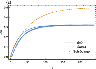
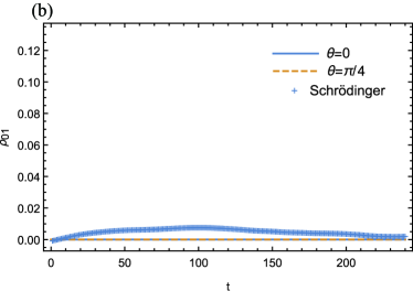
Figure 2: Comparison of the second-order TCL approximation using different projection superoperators and of the numerical solution of the Schrödinger equation. (a) and (b) show the evolution of population $\rho_{00}$ and coherence $\rho_{01}$, respectively. Here $\xi=0$ and the initial state is $|0\rangle_{A}\langle 0|\otimes\Pi^{1}_{\theta}/N$, where $\sin(\theta)=3/5$. Other parameters: $N=60$, $\delta\epsilon=0.5$ and $\alpha=5\times 10^{-3}$.

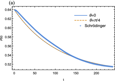
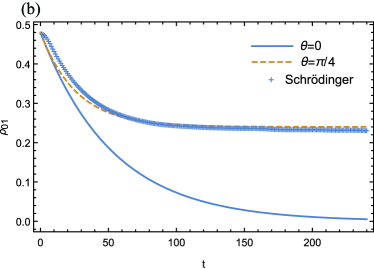
Figure 3: The same as fig. 2 but $\xi=1$ and the initial state is $|\psi\rangle_{A}\langle\psi|\otimes\Pi^{1}$, where $|\psi\rangle=0.6|0\rangle+0.8|1\rangle$.

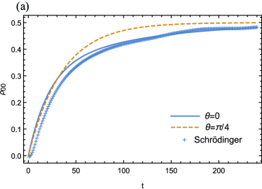
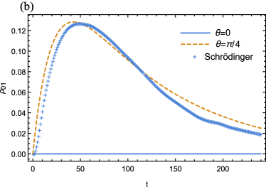
Figure 4: The same as fig. 2 but $\xi=0.5$ and $\alpha=10^{-2}$.

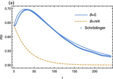
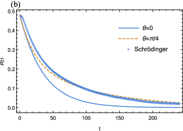
Figure 5: The same as fig. 3 but $\xi=0.5$ and $\alpha=10^{-2}$.

In this section, we compare the results obtained from different projection superoperators [ see appendix B for details] and the numerical solution of the Schrödinger equation.

As shown in fig. 2, when $\xi=0$, two superoperators give the same coherences, which are consistent with the numerical solution. Their populations are totally different. The populations provided by $\Pi^{1,2}$ are pretty accurate through the whole process. In contrast, the projection superoperator $\mathcal{P}_{\theta=\pi/4}$ can’t even provide an accurate steady state. These results are consistent with fig. 1 and the discussions in section III.1: When $\xi=0$, the projection superoperator $\mathcal{P}_{\theta=0}$ is the best for all initial states.

As shown in fig. 3, when $\xi=0$, the populations are the same and consistent with the numerical solution. But the coherences are totally different. The coherences provided by $\mathcal{P}_{\theta=\pi/4}$ are pretty accurate. And the projection superoperator $\mathcal{P}_{\theta=0}$ cannot give an accurate steady state. These results are also consistent with fig. 1 and the discussions in section III.1: When $\xi=1$, the projection superoperator $\mathcal{P}_{\theta=\pi/4}$ is the best for all initial states.

As shown in fig. 4, the populations provided by two projection superoperators are very close. Both give a good approximation. Their coherences are totally different. The coherences given by $\Pi^{+,-}$ are pretty accurate. In contrast, the projection superoperator with $\Pi^{1,2}$ provide a worse approximation. In fig. 5, the populations provided by two projection superoperators are very close. Both give a good approximation. Their coherences are totally different. The populations provided by $\Pi^{1,2}$ are pretty accurate, which can not be achieved by the superoperator $\mathcal{P}_{\theta=\pi/4}$. These results are consistent with fig. 1 and the discussions in section III.1 also: When $\xi=0.5$, the best projection superoperator should depend on initial state and can be selected from $\mathcal{P}_{\theta=0}$ or $\mathcal{P}_{\theta=\pi/4}$.

Comparing fig. 2 with fig. 4 or fig. 3 with fig. 5, one may conclude that a different interaction can completely change the best projection superoperator.

III.5 The failure of homogeneous master equation

The Born-Markov approximation may fail even when the standard Markov condition is fulfilled BGM06 . In their model, the homogeneous master equation obtained by the PS techniques is inaccurate in the low-order expansion. And the populations obtained in the high-order expansion may diverge in the limit $t\to\infty$. In this procedure, a higher order expansion can only improve the approximation for short term, but leads to nonphysical results for longer term. It was proven that the CPS techniques can perfectly solve the problem.

We believe that the root of the problem is that the steady state given by lowest order master equation is totally wrong. If the Markov condition is fulfilled and there is always a steady state, the populations obtained in the lowest order master equation can be generally written as

$$\rho_{i}(t)\equiv\langle i|\rho(t)|i\rangle=A_{i}e^{-\gamma_{1}^{i}t}+\rho^{s}_{i},$$ (49)

where $\rho^{s}_{i}$ is the populations of steady state and all the $\gamma_{1}^{i}$ is positive. In the high-order expansion, the evolution of populations becomes

$$\rho_{i}(t)=A_{i}e^{-\gamma_{1}^{i}t-\gamma_{2}^{i}t^{2}+O(t^{3})}+\rho^{s}_{i}.$$ (50)

Since the master equation of higher order should yield a better approximation for short term, some of $\gamma_{2}^{i}$ must be negative if $\rho^{s}_{i}$ is wrong. However, the negative $\gamma_{2}^{i}$ can lead to divergence for longer term. Hence, a wrong steady state may be the root of the problem. In Ref. BGM06 , the homogeneous master equation obtained by the CPS techniques can yield an accurate steady state, which solves the divergence problem in higher order expansion.

Similar, the homogeneous master equation obtained by the CPS techniques may also fail in some cases. And some of them can be solved by ECPS techniques. For instance, the model of section III.1 with $\xi=0$. Supposing the initial state is

$$\rho_{0}=P_{1}\rho_{A}^{1}\otimes\frac{1}{2N}I+(1-P_{1})\rho_{A}^{2}\otimes\frac{1}{N}\Pi^{+}.$$ (51)

Since $I=\Pi^{1}+\Pi^{2}=\Pi^{+}+\Pi^{-}$, in CPS techniques, one needs projection superoperator $\mathcal{P}_{\theta=\pi/4}$ to obtain a homogeneous master equation. In this approach, the populations of the steady state should be $I/2$ according to Eq. 70. While in ECPS techniques, one can choose $\mathcal{P}_{\theta=0}$ for the term $P_{1}\rho_{A}^{1}\otimes\frac{1}{2N}I$ and $\mathcal{P}_{\theta=\pi/4}$ for the term $(1-P_{1})\rho_{A}^{2}\otimes\frac{1}{N}\Pi^{+}$, to get a homogeneous master equation. Suppose

$$\rho_{A}^{1}=\left(\begin{array}[]{cc}P&0\\ 0&1-P\\ \end{array}\right).$$ (52)

According to Eq. 69, the steady state of the term $P_{1}\rho_{A}^{1}\otimes\frac{1}{2N}I$ should be

$$\rho_{A,s}^{1}=\frac{1}{4}\left(\begin{array}[]{cc}1+2P&0\\ 0&3-2P\\ \end{array}\right).$$ (55)

According to the analysis of section III.3, when $\xi=0$, only the projection superoperator $\mathcal{P}_{\theta=0}$ can always give a good approximation. Hence, the steady state given by CPS techniques would be wrong whenever $P\neq 1/2$. Since the steady state is wrong, the homogeneous master equation provided by the CPS techniques should fail.

The projection superoperator $\mathcal{P}_{\theta=\pi/4}$ can provide a good approximation for some states, such as

$$\rho_{A}^{2}=\frac{1}{2}\left(\begin{array}[]{cc}1&A\\ A^{\dagger}&1\\ \end{array}\right).$$ (56)

In these cases, since the ECPS techniques enable us to choose different projection superoperators for the separated states, it solves the divergence problem in the CPS techniques. But, if $\mathcal{P}_{\theta=\pi/4}$ provides a false steady state to term $(1-P_{1})\rho_{A}^{2}\otimes\frac{1}{N}\Pi^{+}$, then the ECPS techniques can also fail.

In general, the homogeneous master equation from the ECPS techniques is applicable to more general initial state. The results are likely to be convergence. Moreover, it yields more accurate results in lower order equation.

IV Conclusion and outlook

We find that the best projection superoperator can be dependent on initial state. In such circumstances, the ECPS techniques yield a better approximation. Besides that, the relevant part in the ECPS techniques allows for quantum discord between system and environment. Hence, even if an initial state contains quantum discord, one can still obtain a homogeneous master equation in ECPS techniques. Finally, in the framework of homogeneous master equation, we show that the ECPS techniques can yield convergence results for more general initial states.

Since the relevant part in the new approach allows for quantum discord between system and environment, it may be helpful to consider the impact of quantum discord. In fact, the new relevant part can contain all the correlations except for entanglement. Since entanglement is monogamy and the separable state is typical. The ECPS techniques should have wide range of application due to quantum de Finetti’s theorem. Moreover, even for the initial states that contain nontrivial entanglement between system and environment. One may still be able to restrict the inhomogeneous term with monogamy properties of entanglement. The inhomogeneous terms of ECPS techniques deserve further study.

In this paper, we only show that the best projection superoperator can be dependent on the initial state. But the exact relationship is still absent. This issue needs further research. One may solve it by exploring the null space of $\mathcal{P}_{\theta}\mathcal{K}^{2}_{\text{tot}}-\mathcal{K}_{2}(\theta)$.

Appendix A Simplification of the generator

The term $\langle\mathcal{P}_{\theta}\mathcal{L}_{1}(t)\mathcal{L}_{1}(t_{1})\mathcal{P}_{\theta}\rangle$ in $\mathcal{K}^{i}_{1}(t)$ gives

$$\langle\mathcal{P}_{\theta}\mathcal{L}_{1}(t)\mathcal{L}_{1}(t_{1})\mathcal{P}_{\theta}\mathcal{O}\rangle=(1-\xi)^{2}\langle-\mathcal{P}_{\theta}\sigma_{+}[B(t)(\mathcal{P}_{\theta}\mathcal{O})B^{\dagger}(t_{1})]\sigma_{-}+\mathcal{P}_{\theta}\sigma_{+}[B(t)B^{\dagger}(t_{1})(\mathcal{P}_{\theta}\mathcal{O})]\sigma_{-}$$

$$-\mathcal{P}_{\theta}\sigma_{-}[B^{\dagger}(t)(\mathcal{P}_{\theta}\mathcal{O})B(t_{1})]\sigma_{+}+\mathcal{P}_{\theta}\sigma_{-}[B^{\dagger}(t)B(t_{1})(\mathcal{P}_{\theta}\mathcal{O})]\sigma_{+}+\text{H . c}\rangle.$$ (57)

It’s easy to verify that

$$\mathcal{P}_{\theta}B(t)(\mathcal{P}_{\theta}\mathcal{O})B^{\dagger}(t_{1})=\frac{1}{N}\mathcal{P}_{\theta}\text{Tr}(\Pi^{1}B(t)(\mathcal{P}_{\theta}\mathcal{O})B^{\dagger}(t_{1}))\otimes\Pi^{1}$$

$$=\frac{1}{N^{2}}\text{Tr}(\Pi^{1}B(t)\Pi^{2}B^{\dagger}(t_{1}))\mathcal{P}_{\theta}\text{Tr}(\Pi^{2}\mathcal{P}_{\theta}\mathcal{O})\otimes\Pi^{1}=\frac{1}{N^{2}}\text{Tr}(\Pi^{1}B(t)\Pi^{2}B^{\dagger}(t_{1}))\langle\mathcal{P}_{\theta}B(0)(\mathcal{P}_{\theta}\mathcal{O})B^{\dagger}(0)\rangle$$ (58)

and

$$\mathcal{P}_{\theta}B(t)B^{\dagger}(t_{1})(\mathcal{P}_{\theta}\mathcal{O})=\frac{1}{N}\text{Tr}(\Pi^{1}B(t)B^{\dagger}(t_{1}))\mathcal{P}_{\theta}\Pi^{1}(\mathcal{P}_{\theta}\mathcal{O})=\frac{1}{N^{2}}\text{Tr}(\Pi^{1}B(t)B^{\dagger}(t_{1}))\langle\mathcal{P}_{\theta}B(0)B^{\dagger}(0)(\mathcal{P}_{\theta}\mathcal{O})\rangle.$$ (59)

Similar, it’s easy to find that

$$\mathcal{P}_{\theta}B^{\prime}(t)(\mathcal{P}_{\theta}\mathcal{O})B^{\prime\dagger}(t_{1})=\frac{1}{N^{2}}\text{Tr}(\Pi^{+}B^{\prime}(t)\Pi^{-}B^{\prime\dagger}(t_{1}))\langle\mathcal{P}_{\theta}B^{\prime}(0)(\mathcal{P}_{\theta}\mathcal{O})B^{\prime\dagger}(0)\rangle,$$ (60)

$$\mathcal{P}_{\theta}B^{\prime}(t)B^{\prime\dagger}(t_{1})(\mathcal{P}_{\theta}\mathcal{O})=\frac{1}{N^{2}}\text{Tr}(\Pi^{+}B^{\prime}(t)B^{\prime\dagger}(t_{1}))\langle\mathcal{P}_{\theta}B^{\prime}(0)B^{\prime\dagger}(0)(\mathcal{P}_{\theta}\mathcal{O})\rangle.$$

Those two-point environmental correlation function satisfy

$$\langle\text{Tr}(\Pi^{1}B(t)\Pi^{2}B^{\dagger}(t_{1}))\rangle=\langle\text{Tr}(\Pi^{+}B^{\prime}(t)\Pi^{-}B^{\prime\dagger}(t_{1}))\rangle=\langle\text{Tr}(\Pi^{1}B(t)B^{\dagger}(t_{1}))\rangle$$

$$=\langle\text{Tr}(\Pi^{+}B^{\prime}(t)B^{\prime\dagger}(t_{1}))\rangle=\sum_{n_{1},n_{2}}\exp(-i\omega(n_{1},n_{2})\tau)=\gamma N^{2}h(\tau),$$ (61)

where $\tau=t-t_{1}$, $\gamma=2\pi/\delta\epsilon$ and $h(\tau)=\sin^{2}(\delta\epsilon\tau/2)/(\pi\delta\epsilon\tau^{2})$. Combining Eqs. 41, A, A, 59, 60 and A, we obtain

$$\frac{d}{dt}\mathcal{P}_{\theta}\rho_{i}(t)=\mathcal{K}_{2}(\theta)\rho_{i}(t)=\alpha^{2}\gamma\langle\mathcal{P}_{\theta}\mathcal{L}\mathcal{L}\mathcal{P}_{\theta}\rangle\mathcal{P}_{\theta}\rho_{i}(t)=\alpha^{2}\gamma\mathcal{P}_{\theta}(\langle\mathcal{L}_{1}\mathcal{L}_{1}\rangle+\langle\mathcal{L}_{2}\mathcal{L}_{2}\rangle)\mathcal{P}_{\theta}\rho_{i}(t).$$ (62)

The term $\mathcal{P}_{\theta}\langle\mathcal{L}_{1}(t)\mathcal{L}_{1}(t_{1})\rangle$ in $\mathcal{P}_{\theta}\mathcal{K}^{2}_{\text{tot}}$ gives

$$\mathcal{P}_{\theta}\langle\mathcal{L}_{1}(t)\mathcal{L}_{1}(t_{1})\mathcal{\rangle}\mathcal{O}=(1-\xi)^{2}\langle-\mathcal{P}_{\theta}\sigma_{+}[B(t)\mathcal{O}B^{\dagger}(t_{1})]\sigma_{-}+\mathcal{P}_{\theta}\sigma_{+}[B(t)B^{\dagger}(t_{1})\mathcal{O}]\sigma_{-}$$

$$-\mathcal{P}_{\theta}\sigma_{-}[B^{\dagger}(t)\mathcal{O}B(t_{1})]\sigma_{+}+\mathcal{P}_{\theta}\sigma_{-}[B^{\dagger}(t)B(t_{1})\mathcal{O}]\sigma_{+}+\text{H . c}\rangle.$$ (63)

It’s easy to verify that

$$\mathcal{P}_{\theta}\int_{0}^{t}dt_{2}B(t)\rho B^{\dagger}(t_{2})=\frac{1}{N}\mathcal{P}_{\theta}\int_{0}^{t}dt_{2}\text{Tr}(\Pi^{1}B(t)\rho B^{\dagger}(t_{2}))\otimes\Pi^{1},$$ (64)

$$\mathcal{P}_{\theta}\int_{0}^{t}dt_{2}B^{\prime}(t)\rho B^{\prime\dagger}(t_{2})=\frac{1}{N}\mathcal{P}_{\theta}\int_{0}^{t}dt_{2}\text{Tr}(\Pi^{+}B^{\prime}(t)\rho B^{\prime\dagger}(t_{2}))\otimes\Pi^{+}.$$

And

$$\text{Tr}(\Pi^{1}B(t)\rho B^{\dagger}(t_{2}))=\sum_{n_{1},n_{2}}\exp(-i\omega(n_{1},n_{2})\tau)\langle n_{2},2|\rho|n_{2},2\rangle,$$ (65)

$$\text{Tr}(\Pi^{+}B^{\prime}(t)\rho B^{\prime\dagger}(t_{2}))=\sum_{n_{1},n_{2}}\exp(-i\omega(n_{1},n_{2})\tau)\langle n_{2},-|\rho|n_{2},-\rangle.$$

when $\tau\delta\epsilon\gg 1$, the time-dependent part may be approximated as

$$\sum_{n_{1}}\exp(-i\omega(n_{1},n_{2})\tau)\sim N\frac{2\sin(\tau\delta\epsilon/2)e^{-i\tau\delta\epsilon(1/2-n_{2}/N)}}{\tau\delta\epsilon}\sim\gamma N\delta(\tau).$$ (66)

Using this approximation, we have

$$B(t)B^{\dagger}(t_{2})=\sum_{n_{1},n_{2}}\exp(-i\omega(n_{1},n_{2})\tau)|n_{1},1\rangle\langle n_{1},1|\sim\gamma N\delta(\tau)\Pi^{1},$$ (67)

$$B^{\prime}(t)B^{\prime\dagger}(t_{2})=\sum_{n_{1},n_{2}}\exp(-i\omega(n_{1},n_{2})\tau)|n_{1},+\rangle\langle n_{1},+|\sim\gamma N\delta(\tau)\Pi^{+}.$$

Combining Eqs. 46, 67 and A, we obtain

$$\mathcal{P}_{\theta}\mathcal{K}^{2}_{\text{tot}}(t)\rho_{i}(t)=\alpha^{2}\gamma\mathcal{P}_{\theta}\langle\mathcal{L}\mathcal{L}\rangle\rho_{i}(t)=\alpha^{2}\gamma\mathcal{P}_{\theta}(\langle\mathcal{L}_{1}\mathcal{L}_{1}\rangle+\langle\mathcal{L}_{2}\mathcal{L}_{2}\rangle)\rho_{i}(t).$$ (68)

Appendix B The dynamic equation

If set $\theta=0$, Eq. 62 gives

$$\frac{d}{dt}(\rho_{i}^{10,10}+\rho_{i}^{20,20}+\rho_{i}^{11,11}+\rho_{i}^{21,21})=0,$$ (69)

$$\frac{d}{dt}(\rho_{i}^{21,21}+\rho_{i}^{10,10})=0,\quad\frac{d}{dt}(\rho_{i}^{21,21}-\rho_{i}^{10,10})=-\lambda\frac{\xi^{2}}{2}(\rho_{i}^{21,21}-\rho_{i}^{10,10}),$$

$$\frac{d}{dt}(\rho_{i}^{20,20}-\rho_{i}^{11,11})=\lambda(-2+4\xi-\frac{5\xi^{2}}{2})(\rho_{i}^{20,20}-\rho_{i}^{11,11}),$$

$$\frac{d}{dt}(\rho_{i}^{20,21}-\rho_{i}^{10,11})=\lambda(-\frac{1}{2}+\xi-\xi^{2})(\rho_{i}^{20,21}-\rho_{i}^{10,11}),$$

$$\frac{d}{dt}(\rho_{i}^{20,21}+\rho_{i}^{10,11})=\lambda(-\frac{1}{2}+\xi-\frac{3\xi^{2}}{2})(\rho_{i}^{20,21}+\rho_{i}^{10,11}),$$

where $\lambda=\alpha^{2}\gamma N$.

If set $\theta=\pi/4$, Eq. 62 gives

$$\frac{d}{dt}(\rho_{i}^{10,10}+\rho_{i}^{20,20}+\rho_{i}^{11,11}+\rho_{i}^{21,21})=0,\quad\frac{d}{dt}\rho_{i}^{10,21}=0,$$ (70)

$$\quad\frac{d}{dt}(\rho_{i}^{10,20}+\rho_{i}^{10,11}+\rho_{i}^{20,21}+\rho_{i}^{11,21})=-\lambda\frac{1}{2}(\xi-1)^{2}(\rho_{i}^{10,20}+\rho_{i}^{10,11}+\rho_{i}^{20,21}+\rho_{i}^{11,21}),$$

$$\frac{d}{dt}(\rho_{i}^{10,20}-\rho_{i}^{10,11}-\rho_{i}^{20,21}+\rho_{i}^{11,21})=\lambda(-\frac{5\xi^{2}}{2}+\xi-\frac{1}{2})(\rho_{i}^{10,20}-\rho_{i}^{10,11}-\rho_{i}^{20,21}+\rho_{i}^{11,21}),$$

$$\frac{d}{dt}(\rho_{i}^{10,10}+\rho_{i}^{20,20}-\rho_{i}^{11,11}-\rho_{i}^{21,21})=\lambda(-\frac{3\xi^{2}}{2}+2\xi-1)(\rho_{i}^{10,10}+\rho_{i}^{20,20}-\rho_{i}^{11,11}-\rho_{i}^{21,21}),$$

$$\frac{d}{dt}(\rho_{i}^{10,20}-\rho_{i}^{11,21})=\lambda(-\xi^{2}+\xi-\frac{1}{2})(\rho_{i}^{10,20}-\rho_{i}^{11,21}).$$