Equal higher order analysis of an unfitted discontinuous Galerkin method for Stokes flow systems

Abstract.

In this work, we analyze an unfitted discontinuous Galerkin discretization for the numerical solution of the Stokes system based on equal higher-order discontinuous velocities and pressures. This approach combines the best from both worlds, firstly the advantages of a piece-wise discontinuous high–order accurate approximation and secondly the advantages of an unfitted to the true geometry grid around possibly complex objects and/or geometrical deformations. Utilizing a fictitious domain framework, the physical domain of interest is embedded in an unfitted background mesh and the geometrically unfitted discretization is built upon symmetric interior penalty discontinuous Galerkin formulation. To enhance stability we enrich the discrete variational formulation with a pressure stabilization term. Moreover, the present contribution adopts high order ghost penalty strategies to address the ill conditioning of the system matrix caused by small truncated elements with respect to the unfitted boundary. Motivated by continuous unfitted FEM [22, 76, 77] along with other unfitted mesh surveys grounded on discontinuous spaces [11, 45, 46, 75], we use proper velocity and pressure ghost penalties defined on faces of cut cells to establish a robust high-order method, in spite of the cell agglomeration technique usually applied on dG methods. The current presentation should prove valuable in engineering applications where special emphasis is placed on the optimal effective approximation attaining much smaller relative errors in coarser meshes. Inf-sup stability, the optimal order of convergence, and the condition number sensitivity with respect to cut configuration are investigated. Numerical examples verify the theoretical results.

1. Introduction

The overall objective of this paper is to discuss the discontinuous Galerkin method in an unfitted mesh framework. The prominence both of fictitious domain methods, as well as discontinuous Galerkin methods, is easily explained by their relative advantages. Regarding the former, many practical engineering applications involve problems defined in complex domains whose boundary can even be exposed to large topological changes or deformations. Such cases pose severe challenges in the discretization and even result to simulations of diminished quality. For instance, the generation of a suitable conforming mesh is a challenging and computationally intensive task. As a means to bypass such complications, it is instructive to consider the actual computational domain of interest as being embedded in an unfitted background mesh. More precisely, this can be achieved usually via a geometric parametrization of its boundary via level-set geometries, using a fixed Cartesian background and its associated mesh for each new domain configuration. This approach avoids the need to remesh, as well as the need to develop a reference domain formulation in many applications and methodologies, as typically done in fitted grid FEMs.

The discontinuous Galerkin method is a robust finite element method that is very well suited to handling complicated geometries with unfitted to the true geometry and/or unstructured meshes. DG methods generalize the continuous finite element framework by relaxing the continuity constraints at inter-element boundaries, thus providing the tools to manipulate potential jumps via numerical fluxes [35]. Such an approach results in additional flexibility in the design of shape functions and enables the use of different polynomial degrees of approximation on adjacent elements, as well as incorporates interfaces between non matching grids and evolving domains [2, 4, 10, 40, 42]. Hence, the main motivation for using dG methods in fluid flow problems lies in their robustness in convection-dominated regimes, their conservation properties, and their great flexibility in the mesh-design. Since less communication is required between neighbouring mesh cells, the method is more amenable in parallel computing [72, 93] and it is highly attractive in $hp$-adaptive strategies [3, 29, 89, 94] where mesh refinement can be achieved without the continuity restrictions customary in standard finite element methods.

A higher order analysis of an unfitted discontinuous approach for the Stokes system combines the best of the two methodologies and shows better stability properties than continuous Galerkin, allowing high–order accurate approximations within a geometrically unfitted setting. A major challenge in the unfitted mesh case is that stability and approximations properties as well as the conditioning of the system matrix can be severely impacted by the presence of small cut elements. A possible remedy is to introduce a stabilization term, the so-called ghost penalty term, which prevents the ill-conditioning of the discrete problem. So far, there are few examples in the literature of high-order stabilized unfitted FEM where Stokes equation is considered. In [22, 47] unfitted finite element pressure–velocity couplings for the Stokes problem are employed, in [56] the authors utilize high–order piecewise polynomials to develop a cut finite element method on composite meshes, while [66] is based on an isoparametric mapping reconstruction for high accurate geometry approximations. On the other hand, unfitted dG have mostly been relied on cell agglomeration to deal with the small cut element problem. For instance, in [18] a hybrid high-order (HHO) method has been recently designed and analyzed to approximate the Stokes interface problem on unfitted meshes and in [81] the compressible Navier–Stokes equations.

Regardless to the cell merging approach, the present work aims to advocate ghost–penalty–type techniques in a higher order analysis of an unfitted dG setting for the Stokes system. In this respect, we augment the discrete system with additional boundary zone ghost penalty terms for both velocity and pressure fields so as to circumvent small cut configuration problems. These terms act on the jumps of the normal derivatives at faces associated with cut elements and ensure that the condition number is uniformly bounded independently of how the boundary intersects the mesh. Moreover, a fully stabilized scheme is guaranteed by penalizing the pressure jumps across interfaces. To the authors’ best knowledge some original introduction of pressure jump/ghost penalties for the Stokes system has only been provided in [11, 17] and also some recent contributions on cut dG in [45, 46, 75].

Various stabilized finite elements for the Stokes system on fictitious domains have been analyzed in [7, 17, 22, 43, 76, 77] and also extended to the Stokes interface problem in [52, 63]. A number of different face-based ghost-penalty stabilizations on cut meshes combined with the continuous interior penalty method has been elaborated in [19, 78, 96] and in [91] for the transient convection–dominant incompressible Navier–Stokes equations. Analogous work for elliptic boundary value and interface problems has been carried out in [20, 21]. On the other hand, unfitted dG benefits from the favorable conservation and stability properties of classical dG to solve several boundary and interface problems [10, 38, 55, 95] along with two–phase flows [41, 53, 64, 65, 81, 92]. A dG variant utilizing divergence–free vector fields for the velocity and continuous pressure approximations for the Stokes and incompressible Navier–Stokes equations has been studied in [8, 61], respectively. Local Discontinuous Galerkin (LDG) rationales based on mixed formulations of piecewise solenoidal polynomial velocities and hybrid pressures have been studied in [30, 31, 32, 34], and also in [80] under interior penalty formulations. Mixed $hp$-discontinuous Galerkin methods for the Stokes problem with a stabilization term penalizing the pressure jumps have been treated in [89, 94]. In a vast and non–exhaustive list in the literature on various dG methods, see also [6, 27, 28, 33, 51, 70] and the references therein.

Fictitious domain methods have a long history, dating back to the pioneering work of Peskin [85] and are currently enjoying great popularity, having been successfully applied to a variety of problems. Several improved variants can be found in the recent literature, including such methods as the ghost–cell finite difference method [97], cut–cell volume method [84], immersed interface [68], ghost fluid [12], shifted boundary methods [73], $\phi$–FEM [37], and CutFEM [5, 16, 20, 21, 25, 26, 49, 62, 71], among others. For a comprehensive overview of this research area, the interested reader is referred to the review paper [79] and also to the recent book volume [13] based on the proceedings of the UCL Workshop 2016. Considerable impetus for such widespread investigations has been provided by applications in fluids flow or in the context of reduced order modeling for parametrically–dependent domains [57, 58, 59, 60]. In such cases, immersed and embedded methods compare favorably to standard FEM, providing simple and efficient schemes for the numerical approximation of PDEs in both cases of static and evolving geometries.

Many unfitted variants of discontinuous Galerkin methods have been proposed in the literature as a competitive approaches for simulations in complex and evolving domains [88]. One of the first applications involved an elliptic model problem [9], while elliptic interface problems have been discretized via an hp discontinuous Galerkin method [74], an extension of the local dG method [95], and a high–order hybridizable dG method [36, 54]. In fact, an unfitted dG method was shown to compare favorably to standard dG–FEM [82], providing a flexible and accurate alternative to solve the electroencephalography forward problem. Moreover, we refer to Saye’s important work [88] in which a numerical quadrature algorithm has been applied to a high-order embedded boundary dG method on curved domains and also to [86, 87] for a high-order accurate implicit mesh dG to facilitate precise computation of interfacial fluid flows in evolving geometries. An extension to a parabolic test case has been presented in [10]. More recently, motivated from PDEs arising from conservation laws on evolving surfaces, an unfitted dG approach was developed for advection problems [40]. Other applications include the linear transport equation [39], the Laplace–Beltrami operator on surfaces [24] and mixed–dimensional, coupled bulk–surface problems [75]. In the context of Stokes problems with void or material interfaces, previous efforts include an eXtended hybridizable dG (X-HDG) method [44] combining the hybridizable dG method with an eXtended finite element strategy, considering heaviside enrichment on cut faces/elements.

Our paper is organized as follows. We start with the Stokes flow model problem and the necessary preliminaries in Section 2. The various components of the stabilized unfitted discontinuous Galerkin discretization based on equal higher order discontinuous velocities and pressures are discussed in subsection 2.2 in detail. Approximation results needed for the analysis of the method are collected in Section 3. Section 4 is devoted to stability estimates and the derivation of the discrete inf–sup condition, followed by a–priori error estimates in Section 5. Our theoretical analysis of the method is completed in Section 6, showing that the condition number of the stiffness matrix is uniformly bounded, independently of how the background mesh cuts the boundary. The paper concludes with some numerical tests in Section 7 which verify the theoretical convergence rates, the accuracy and the geometrical robustness of the method.

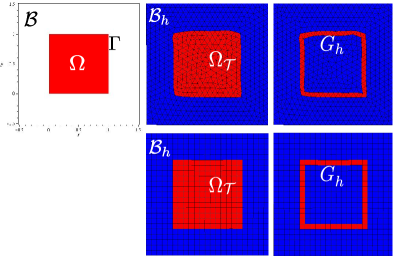
Figure 1. The original square domain $\mathrm{\Omega}$ (left picture) and its boundary $\mathrm{\Gamma}$ are represented implicitly by the level-set function $\phi(x,y)$ in (7.1) and they are designated by the red colored area. The extended computational domain $\mathrm{\Omega}_{\mathcal{T}}$ is visualized in the middle picture, and it is covered by the active part of the background mesh $\mathcal{B}_{h}$ colored in red. The subset $G_{h}$ of elements in $\mathcal{B}_{h}$ that intersect the boundary $\mathrm{\Gamma}$ is shown in red at the right picture.

2. The model problem and preliminaries

2.1. Problem formulation

The steady Stokes equations for an incompressible viscous fluid confined in an open, bounded domain $\mathrm{\Omega}\subset\mathbb{R}^{d}$ ($d=2,3$) with Lipschitz boundary $\mathrm{\Gamma}=\partial\mathrm{\Omega}$ can be expressed in the form

$$-\Delta\mathbf{u}+\nabla p = \mathbf{f}\quad\,\,\,\,\,\textrm{in}\,\,\,\mathrm{\Omega},$$

(2.1) $$\nabla\cdot\mathbf{u} = 0\quad\,\,\,\,\,\textrm{in}\,\,\,\mathrm{\Omega},$$

$$\mathbf{u} = 0\qquad\textrm{on}\,\,\,\mathrm{\Gamma}.$$

Here $\mathbf{u}=(u_{1},\dots,u_{d}):\mathrm{\Omega}\rightarrow\mathbb{R}^{d}$ ($d=2,3$) and $p:\mathrm{\Omega}\rightarrow\mathbb{R}$ denote the velocity and pressure fields, and $\mathbf{f}\in\left[L^{2}(\mathrm{\Omega})\right]^{d}$ is a forcing term. Since the pressure is determined by (2.1) up to an additive constant, we assume $\int_{\mathrm{\Omega}}p\,\mathrm{d}x=0$ to uniquely determine $p$. Hence, in the following we will consider for pressure the standard space

$$L_{0}^{2}(\mathrm{\Omega}):=\Big{\{}q\in L^{2}(\mathrm{\Omega}):\int_{\mathrm{\Omega}}q\,{\color[rgb]{0,0,0}\mathrm{d}x}=0\Big{\}}$$

of square–integrable functions with zero average over $\mathrm{\Omega}$.

Defining for all $\mathbf{u},\mathbf{v}\in V:=[H_{0}^{1}(\mathrm{\Omega})]^{d}$ and $p\in Q:=L_{0}^{2}(\mathrm{\Omega})$ the bilinear forms

(2.2) $$a(\mathbf{u},\mathbf{v})=\int_{\mathrm{\Omega}}\nabla\mathbf{u}:\nabla\mathbf{v}\,{\color[rgb]{0,0,0}\mathrm{d}\mathbf{x}},\quad b(\mathbf{v},p)=-\int_{\mathrm{\Omega}}p\nabla\cdot\mathbf{v}\,{\color[rgb]{0,0,0}\mathrm{d}\mathbf{x}},$$

a weak solution to (2.1) is a pair $(\mathbf{u},p)\in[H_{0}^{1}(\mathrm{\Omega})]^{d}\times L_{0}^{2}(\mathrm{\Omega})=V\times Q$, such that

(2.3) $$A(\mathbf{u},p;\mathbf{v},q)=\int_{\mathrm{\Omega}}\mathbf{f}\cdot\mathbf{v}\,{\color[rgb]{0,0,0}\mathrm{d}\mathbf{x}},\ \ \textrm{for all test functions}\ \ (\mathbf{v},q)\in V\times Q,$$

with

$$A(\mathbf{u},p;\mathbf{v},q)=a(\mathbf{u},\mathbf{v})+b(\mathbf{u},q)+b(\mathbf{v},p).$$

The well–posedness of (2.3) is standard [35].

2.2. Discretization via an unfitted discontinuous Galerkin method

Implementation of an unfitted discontinuous Galerkin method for the discretization of (2.3) requires a fixed background domain $\mathcal{B}$ which contains $\mathrm{\Omega}$. Let $\mathcal{B}_{h}$ be its corresponding shape–regular mesh, the active mesh

$$\mathcal{T}_{h}=\left\{T\in\mathcal{B}_{h}:T\cap\mathrm{\Omega}\neq\emptyset\right\}$$

is the minimal submesh of $\mathcal{B}_{h}$ which covers $\mathrm{\Omega}$ and is, in general, unfitted to its boundary $\mathrm{\Gamma}$. As usual, the subscript $h=\max_{T\in\mathcal{B}_{h}}h_{T}=\max_{T\in\mathcal{B}_{h}}\mathrm{diam}(T)$ indicates the global mesh size. Finite element spaces for $\mathbf{u}$ and $p$ will be built upon the extended domain $\mathrm{\Omega}_{\mathcal{T}}=\bigcup_{T\in\mathcal{T}_{h}}T$ which corresponds to $\mathcal{T}_{h}$. The set of interior faces in the active background mesh is denoted

$$\mathcal{F}_{h}^{int}=\left\{F=T^{+}\cap T^{-}:T^{+},T^{-}\in\mathcal{T}_{h}\right\}.$$

Fictitious domain methods, as well as, discontinuous Galerkin related schemes need Dirichlet boundary conditions at $\mathrm{\Gamma}$ to be weakly satisfied through a variant of Nitsche’s method since the mesh does not align with the boundary of the physical domain. Moreover, when Nitsche’s approach is applied in the discontinuous Galerkin framework, the continuity of the solution across inter-element boundaries can be attained allowing for independent approximations on different elements and thus, resulting to a consistent discrete scheme [11, 44, 45, 46]. On the other hand, coercivity over the whole computational domain $\mathrm{\Omega}_{\mathcal{T}}$ is ensured by means of additional ghost penalty terms which act on the gradient jumps in the boundary zone; see, for instance, [21, 22, 57, 76]. The submesh consisting of all cut elements is denoted

$${G}_{h}:=\{T\in\mathcal{T}_{h}:T\cap\mathrm{\Gamma}\neq\emptyset\}$$

and the relevant set of faces upon which ghost penalty will be applied is given by

$$\mathcal{F}_{G}:=\left\{F:F\textrm{ is a face of }T\in G_{h},F\,{\color[rgb]{0,0,0}\nsubseteq}\,\partial\mathrm{\Omega}_{\mathcal{T}}\right\}.$$

We recall that the boundary $\mathrm{\Gamma}$ is well resolved by the mesh $\mathcal{T}_{h}$ if the following assumptions are satisfied from [17, 76]:

• The intersection between $\mathrm{\Gamma}$ and a facet $F\in\mathcal{F}_{h}^{int}$ is simply connected; that is, $\mathrm{\Gamma}$ does not cross an interior facet multiple times.

• For each element $T$ intersected by $\mathrm{\Gamma}$, there exists a plane $S_{T}$ and a piecewise smooth parametrization $\mathrm{\Phi}:S_{T}\cap T\to\mathrm{\Gamma}\cap T$.

• We assume that there is an integer $N>0$ such that for each element $T\in G_{h}$, there exists an element $T^{\prime}\in\mathcal{T}_{h}\setminus G_{h}$ and at most $N$ elements $\{T\}_{j=1}^{N}$ such that $T_{1}=T$, $T_{N}=T^{\prime}$ and $T_{j}\cap T_{j+1}\in\mathcal{F}_{h}^{int}$, $j=1,\ldots,N-1$. In other words, the number of facets to be crossed in order to “walk” from a cut element $T$ to a non-cut element $T^{\prime}\subset\mathrm{\Omega}$ is bounded.

To define an unfitted discontinuous Galerkin discretization for the Stokes problem (2.3), we consider equal–order, elementwise discontinuous polynomial finite element pressure and velocity spaces of order $k\geq 1$:

$$V_{h} :=\Big{\{}\mathbf{w}_{h}\in\Big{(}L^{2}(\mathrm{\Omega}_{\mathcal{T}})\Big{)}^{d}:\mathbf{w}_{h}|_{T}\in\Big{(}\mathcal{P}^{k}(T)\Big{)}^{d},T\in\mathcal{T}_{h}\Big{\}}\quad(d=2,3)$$

$$Q_{h} :=\Big{\{}w_{h}\in L^{2}(\mathrm{\Omega}_{\mathcal{T}}):{\color[rgb]{0,0,0}\int_{\mathrm{\Omega}}w_{h}\,\mathrm{d}x=0},\,\,w_{h}|_{T}\in\mathcal{P}^{k}(T),T\in\mathcal{T}_{h}\Big{\}}.$$

Moreover, recall the definition

$$\left\{v\right\}:=\frac{1}{2}\left(v^{+}+v^{-}\right),\quad\quad\left\{\mathbf{v}\right\}:=\frac{1}{2}\left(\mathbf{v}^{+}+\mathbf{v}^{-}\right),$$

of the average operator $\left\{\cdot\right\}$ across an interior face $F$ for $v$, $\mathbf{v}$ scalar and vector–valued functions on $\mathcal{T}_{h}$ respectively, where $v^{\pm}$ (resp. $\mathbf{v}^{\pm}$) are the traces of $v$ (resp. $\mathbf{v}$) on $F=T^{+}\cap T^{-}$ from the interior of $T^{\pm}$. More precisely, $v^{\pm}(\mathbf{x})=\lim_{t\rightarrow 0^{+}}v(\mathbf{x}{\color[rgb]{0,0,0}\mp}t{\bf n}_{F})$ for $\mathbf{x}\in F$ and ${\bf n}_{F}$ the outward–pointing unit normal vector to $F$. The jump operator $[\![\cdot]\!]$ across $F$ is defined respectively by

$$[\![v]\!]:=v^{+}-v^{-},\quad\quad[\![\mathbf{v}]\!]:=\mathbf{v}^{+}-\mathbf{v}^{-}.$$

With these definitions in place, we are now ready to formulate a discrete counterpart of (2.3) employing an unfitted discontinuous Galerkin method. The symmetric interior penalty discretizations of the diffusion term and the pressure–velocity coupling in (2.2) lead to the bilinear forms

$$a_{h}(\mathbf{u}_{h},\mathbf{v}_{h})=\int_{\mathrm{\Omega}}\nabla\mathbf{u}_{h}:\nabla\mathbf{v}_{h}\,{\color[rgb]{0,0,0}\mathrm{d}\mathbf{x}}-\sum_{F\in\mathcal{F}_{h}^{int}}\int_{F\cap\mathrm{\Omega}}\left(\left\{\nabla\mathbf{u}_{h}\right\}\cdot{\bf n}_{F}[\![\mathbf{v}_{h}]\!]+\left\{\nabla\mathbf{v}_{h}\right\}\cdot{\bf n}_{F}[\![\mathbf{u}_{h}]\!]\right)\,{\color[rgb]{0,0,0}\mathrm{d}s}$$

$$\quad\quad\quad\quad\quad\quad\quad\quad-\int_{\mathrm{\Gamma}}\mathbf{u}_{h}\nabla\mathbf{v}_{h}\cdot\mathbf{n}_{\mathrm{\Gamma}}\,\,{\color[rgb]{0,0,0}\mathrm{d}s}-\int_{\mathrm{\Gamma}}\mathbf{v}_{h}\nabla\mathbf{u}_{h}\cdot\mathbf{n}_{\mathrm{\Gamma}}\,\,{\color[rgb]{0,0,0}\mathrm{d}s}+\beta h^{-1}\int_{\mathrm{\Gamma}}\mathbf{u}_{h}\mathbf{v}_{h}\,{\color[rgb]{0,0,0}\mathrm{d}s}$$

$$\qquad\qquad\quad\quad\quad\quad\quad\quad\quad\quad\quad\quad\quad\quad\quad\quad\quad\quad+\beta h^{-1}\sum_{F\in\mathcal{F}_{h}^{int}}\int_{F\cap\mathrm{\Omega}}[\![\mathbf{u}_{h}]\!][\![\mathbf{v}_{h}]\!]\,{\color[rgb]{0,0,0}\mathrm{d}s},$$

$$b_{h}(\mathbf{v}_{h},p_{h})=-\int_{\mathrm{\Omega}}p_{h}\nabla\cdot\mathbf{v}_{h}\,{\color[rgb]{0,0,0}\mathrm{d}\mathbf{x}}+\sum_{F\in\mathcal{F}_{h}^{int}}\int_{F\cap\mathrm{\Omega}}[\![\mathbf{v}_{h}]\!]\cdot\mathbf{n}_{F}\left\{p_{h}\right\}{\color[rgb]{0,0,0}\mathrm{d}s}+\int_{\mathrm{\Gamma}}\mathbf{v}_{h}\cdot\mathbf{n_{\mathrm{\Gamma}}}p_{h}\,{\color[rgb]{0,0,0}\mathrm{d}s}$$

respectively. It is important to mention that in an abuse of notation whenever $\nabla w_{h}$ is used for functions that lay in the discontinuous Galerkin space, i.e. $w_{h}\notin H^{1}(\mathrm{\Omega}_{\mathcal{T}})$, it corresponds to the broken gradient such that $(\nabla w_{h})|_{T}=\nabla(w_{h}|_{T})$ for all $T\in\mathcal{T}_{h}$. The same applies for the broken divergence operator $\nabla\cdot w_{h}$ defined element–wise.

The symmetric interior penalty parameter $\beta>0$ in the definition of $a_{h}(\cdot,\cdot)$ is chosen sufficiently large to ensure stability of the method and will be made precise later; see Lemma 4.2 and its proof below. For future reference, note that element–wise integration by parts in the previous forms yields the equivalent formulations

$$a_{h}(\mathbf{u}_{h},\mathbf{v}_{h}) =-\int_{\mathrm{\Omega}}\Delta\mathbf{u}_{h}\cdot\mathbf{v}_{h}\,{\color[rgb]{0,0,0}\mathrm{d}\mathbf{x}}+\sum_{F\in\mathcal{F}_{h}^{int}}\int_{F\cap\mathrm{\Omega}}[\![\nabla\mathbf{u}_{h}]\!]\cdot\mathbf{n}_{F}\left\{\mathbf{v}_{h}\right\}\,{\color[rgb]{0,0,0}\mathrm{d}s}$$

$$\quad-\sum_{F\in\mathcal{F}_{h}^{int}}\int_{F\cap\mathrm{\Omega}}\left\{\nabla\mathbf{v}_{h}\right\}\cdot{\bf n}_{F}[\![\mathbf{u}_{h}]\!]\,{\color[rgb]{0,0,0}\mathrm{d}s}-\int_{\mathrm{\Gamma}}\mathbf{u}_{h}\nabla\mathbf{v}_{h}\cdot\mathbf{n}_{\mathrm{\Gamma}}\,{\color[rgb]{0,0,0}\mathrm{d}s}$$

(2.4) $$\quad\quad+\beta h^{-1}\int_{\mathrm{\Gamma}}\mathbf{u}_{h}\mathbf{v}_{h}\,{\color[rgb]{0,0,0}\mathrm{d}s}+\beta h^{-1}\sum_{F\in\mathcal{F}_{h}^{int}}\int_{F\cap\mathrm{\Omega}}[\![\mathbf{u}_{h}]\!][\![\mathbf{v}_{h}]\!]\,{\color[rgb]{0,0,0}\mathrm{d}s},$$

(2.5) $$b_{h}(\mathbf{v}_{h},p_{h}) =\int_{\mathrm{\Omega}}\mathbf{v}_{h}\cdot\nabla p_{h}\,{\color[rgb]{0,0,0}\mathrm{d}\mathbf{x}}-\sum_{F\in\mathcal{F}_{h}^{int}}\int_{F\cap\mathrm{\Omega}}\left\{\mathbf{v}_{h}\right\}\cdot\mathbf{n}_{F}[\![p_{h}]\!]\,{\color[rgb]{0,0,0}\mathrm{d}s},$$

which will be useful for asserting the consistency of the method.

Owing to the use of equal–order, discontinuous interpolation spaces, the essential inf–sup stability condition is violated. To overcome this difficulty and enhance stability, extra terms need to be added in the dG variational formulation where a standard stabilization involves the pressure face jump penalty

(2.6) $$c_{h}(p_{h},q_{h})=\gamma\sum_{F\in\mathcal{F}_{h}^{int}}\int_{F\cap\mathrm{\Omega}}h_{F}[\![p_{h}]\!][\![q_{h}]\!]\,\mathrm{d}s,$$

where $\gamma$ is a positive parameter and $h_{F}=\min\left\{h_{T},h_{T^{\prime}}\right\}$ for $F=T\cap T^{\prime}\in\mathcal{F}_{h}^{int}$. Some surveys on finite element methods allowing for equal–order velocity and pressure approximations in conjunction with an interior penalty method can be found, e.g., in [14, 15, 32, 33] with an extensive study in the monograph [35] on dG methods by Di Pietro and Ern.

Finally, to extend stabilization on cut elements as well, we also consider the form [22, 76]

(2.7) $$J_{h}(\mathbf{u}_{h},p_{h};\mathbf{v}_{h},q_{h})=j_{u}(\mathbf{u}_{h},\mathbf{v}_{h})-j_{p}(p_{h},q_{h}).$$

Here, the additional velocity and pressure ghost penalty forms are defined by

(2.8) $$j_{u}(\mathbf{u}_{h},\mathbf{v}_{h}) =\gamma_{\mathbf{u}}\sum_{j=1}^{d}\sum_{F\in\mathcal{F}_{G}}{\color[rgb]{0,0,0}\sum_{i=0}^{k}}\int_{F}h_{F}^{2i-1}[\![\partial_{\mathbf{n}_{F}}^{i}u_{h,j}]\!][\![\partial_{\mathbf{n}_{F}}^{i}v_{h,j}]\!]\,{\color[rgb]{0,0,0}\mathrm{d}s},$$

(2.9) $$j_{p}(p_{h},q_{h}) =\gamma_{p}\sum_{F\in\mathcal{F}_{G}}{\color[rgb]{0,0,0}\sum_{i=0}^{k}}\int_{F}h_{F}^{2i+1}[\![\partial_{\mathbf{n}_{F}}^{i}p_{h}]\!][\![\partial_{\mathbf{n}_{F}}^{i}q_{h}]\!]\,{\color[rgb]{0,0,0}\mathrm{d}s},$$

where $\partial_{\mathbf{n}}^{i}v$ is the $i$-th normal derivative given by $\partial_{\mathbf{n}}^{i}v:=\sum_{|\alpha|=i}\frac{1}{\alpha!}D^{\alpha}v(x)\mathbf{n}^{\alpha}$ for multi-index $\alpha=(\alpha_{1},\ldots,\alpha_{d})$, $|\alpha|=\sum_{i=1}^{d}\alpha_{i}$ and $\alpha!=\prod_{i=1}^{d}\alpha_{i}!$. Let also $\mathbf{n}^{\alpha}:=n_{1}^{\alpha_{1}}n_{2}^{\alpha_{2}}\cdots n_{d}^{\alpha_{d}}$ and $D^{\alpha}:=\frac{\partial^{|\alpha|}}{\partial^{\alpha_{1}}\partial^{\alpha_{2}}\cdots\partial^{\alpha_{d}}}$.

The ghost penalty terms defined in (2.8) and (2.9) are designed to provide sufficient control over the discrete velocity and pressure norms in the extended domain $\mathrm{\Omega}_{\mathcal{T}}$. In particular, when deriving geometrically robust condition numbers, it is critical for the velocity ghost penalty to penalize the lowest order contribution of the form $\int_{F}h_{F}^{-1}[\![\mathbf{u}_{h}]\!][\![\mathbf{v}_{h}]\!]\,\mathrm{d}s$ and also the higher-order normal derivatives up to the polynomial degree on the entire face in the vicinity of the boundary. The a priori error estimate would still go through with suitably defined discrete velocity norms. Similarly, the same hold for the pressure ghost penalty in (2.9). For further discussion of a number of issues regarding suitable ghost penalties for dG based discretization, we refer to Gürkan and Massing in [45]. The parameters $\gamma_{\mathbf{u}}$ and $\gamma_{p}$ in (2.8) and (2.9) are positive stabilization constants. More details regarding the CutFEM discretization of the Stokes system can be found in [22].

Using the previous ingredients, an extended mesh discontinuous Galerkin method for (2.3) now reads as follows: Find $(\mathbf{u}_{h},p_{h})\in V_{h}\times Q_{h}$, such that

(2.10) $$A_{h}(\mathbf{u}_{h},p_{h};\mathbf{v}_{h},q_{h})+J_{h}(\mathbf{u}_{h},p_{h};\mathbf{v}_{h},q_{h})={\color[rgb]{0,0,0}L_{h}(\mathbf{v}_{h})},\ \ \textrm{for all}\ \ (\mathbf{v}_{h},q_{h})\in V_{h}\times Q_{h}.$$

The bilinear and linear forms $A_{h}$ and $L_{h}$ are defined by

(2.11) $$A_{h}(\mathbf{u}_{h},p_{h};\mathbf{v}_{h},q_{h}) =a_{h}(\mathbf{u}_{h},\mathbf{v}_{h})+b_{h}(\mathbf{u}_{h},q_{h})+b_{h}(\mathbf{v}_{h},p_{h})-{\color[rgb]{0,0,0}c_{h}(p_{h},q_{h})},$$

(2.12) $${\color[rgb]{0,0,0}L_{h}(\mathbf{v}_{h})} ={\color[rgb]{0,0,0}\int_{\mathrm{\Omega}}\mathbf{f}\cdot\mathbf{v}_{h}\,\mathrm{d}\mathbf{x}.}$$

A similar method without stabilization has been presented in [38].

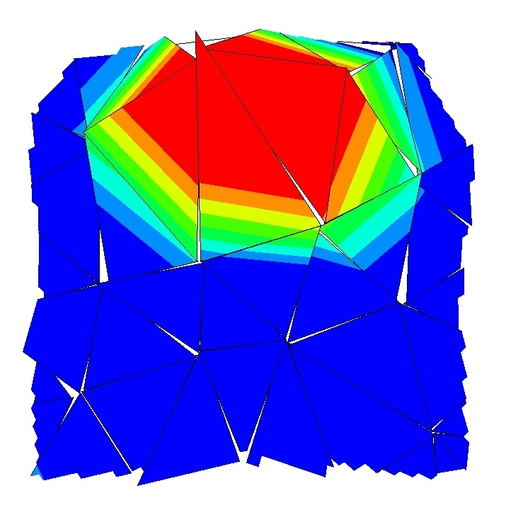
(a) $h_{0}=2^{-2}$

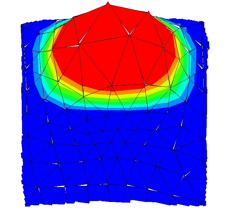
(b) $h_{1}=2^{-3}$

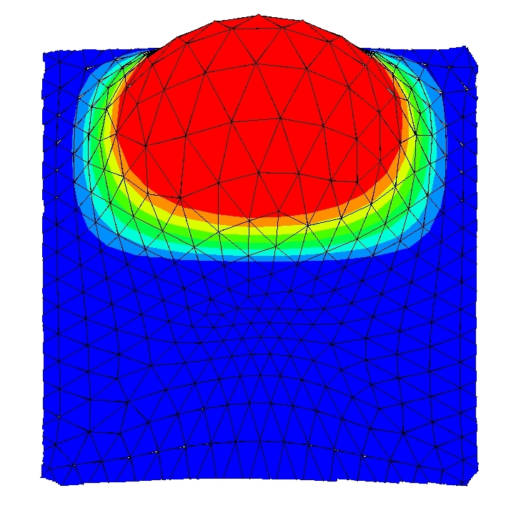
(c) $h_{2}=2^{-4}$

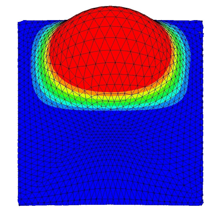
(d) $h_{3}=2^{-5}$

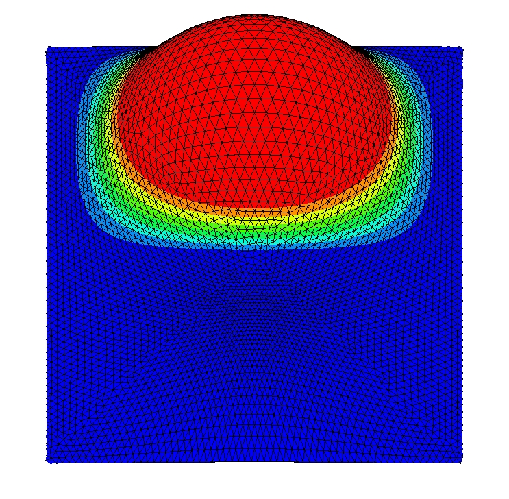
(e) $h_{4}=2^{-6}$

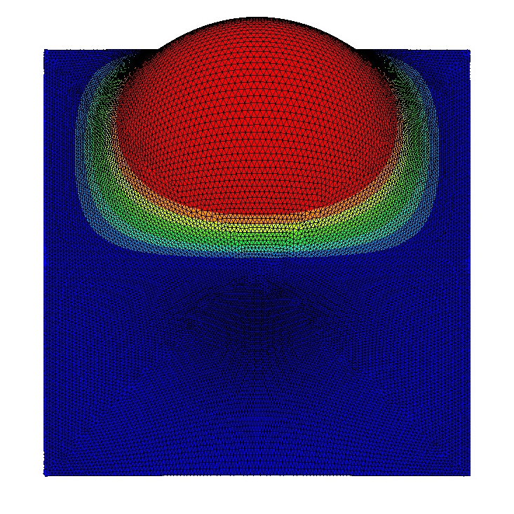
(f) $h_{5}=2^{-7}$

Figure 2. Numerical approximation of the first component of the velocity solution visualized for a sequence of successively refined tessellations of the background domain $\mathcal{B}=\left[-0.5,1.5\right]^{2}$ with mesh parameters $h_{\ell}=2^{-\ell-2}$ ($\ell=0,\dots,5$) and $P_{1}-P_{1}$ finite elements.

3. Approximation properties

Throughout this manuscript, standard Sobolev norms and semi–norms on a domain $\mathcal{X}$ for $s\in\mathbb{N}$ will be denoted by $\left\|\cdot\right\|_{s,\mathcal{X}}$ and $|\cdot|_{s,\mathcal{X}}$ respectively, omitting the index in case $s=0$. A–priori error bounds for the proposed unfitted dG method will be proved with respect to the following mesh–dependent norms:

$${\left|\kern-1.07639pt\left|\kern-1.07639pt\left|\mathbf{v}\right|\kern-1.07639pt\right|\kern-1.07639pt\right|}^{2}=\left\|\nabla\mathbf{v}\right\|^{2}_{\mathrm{\Omega}}+\left\|h^{-1/2}\mathbf{v}\right\|^{2}_{\mathrm{\Gamma}}+\left\|h^{1/2}\nabla\mathbf{v}\cdot\mathbf{n}_{\mathrm{\Gamma}}\right\|^{2}_{\mathrm{\Gamma}}+\sum_{F\in\mathcal{F}_{h}^{int}}\left\|h^{-1/2}[\![\mathbf{v}]\!]\right\|^{2}_{F\cap\mathrm{\Omega}}+$$

$$\quad\quad\quad\quad\quad\quad\quad\quad\quad\quad\quad\quad\quad\quad\quad\quad\quad\quad\quad\quad\quad+\sum_{T\in\mathcal{T}_{h}}\left\|h^{1/2}\nabla\mathbf{v}|_{T}\cdot\mathbf{n}_{\partial T}\right\|_{\partial T\cap\mathrm{\Omega}}^{2},$$

$${\color[rgb]{0,0,0}{\left|\kern-1.07639pt\left|\kern-1.07639pt\left|p\right|\kern-1.07639pt\right|\kern-1.07639pt\right|}^{2}=\left\|p\right\|^{2}_{\mathrm{\Omega}}\,\,\,+\left\|h^{1/2}p\right\|^{2}_{\mathrm{\Gamma}}+\sum_{T\in\mathcal{T}_{h}}\left\|h^{1/2}p\right\|^{2}_{\partial T\cap\mathrm{\Omega}}},$$

$${\left|\kern-1.07639pt\left|\kern-1.07639pt\left|(\mathbf{v},p)\right|\kern-1.07639pt\right|\kern-1.07639pt\right|}^{2}={\left|\kern-1.07639pt\left|\kern-1.07639pt\left|\mathbf{v}\right|\kern-1.07639pt\right|\kern-1.07639pt\right|}^{2}+{\left|\kern-1.07639pt\left|\kern-1.07639pt\left|p\right|\kern-1.07639pt\right|\kern-1.07639pt\right|}^{2}.$$

To investigate stability, we will also make use of the following norms on the extended domain $\mathrm{\Omega}_{\mathcal{T}}$ for the discrete velocity and pressure approximations and their product space:

$${\left|\kern-1.07639pt\left|\kern-1.07639pt\left|\mathbf{v}\right|\kern-1.07639pt\right|\kern-1.07639pt\right|}^{2}_{V}=\left\|\nabla\mathbf{v}\right\|^{2}_{\mathrm{\Omega}_{\mathcal{T}}}+\left\|h^{-1/2}\mathbf{v}\right\|^{2}_{\mathrm{\Gamma}}+\sum_{F\in\mathcal{F}_{h}^{int}}\left\|h^{-1/2}[\![\mathbf{v}]\!]\right\|^{2}_{F\cap\mathrm{\Omega}},$$

$${\left|\kern-1.07639pt\left|\kern-1.07639pt\left|p_{h}\right|\kern-1.07639pt\right|\kern-1.07639pt\right|}^{2}_{Q}=\left\|p\right\|^{2}_{\mathrm{\Omega}_{\mathcal{T}}}\,\,\,$$

$${\left|\kern-1.07639pt\left|\kern-1.07639pt\left|(\mathbf{v},p)\right|\kern-1.07639pt\right|\kern-1.07639pt\right|}^{2}_{V,Q}={\left|\kern-1.07639pt\left|\kern-1.07639pt\left|\mathbf{v}\right|\kern-1.07639pt\right|\kern-1.07639pt\right|}_{V}^{2}+{\left|\kern-1.07639pt\left|\kern-1.07639pt\left|p\right|\kern-1.07639pt\right|\kern-1.07639pt\right|}^{2}_{Q}.$$

We should note that the norms ${\left|\kern-1.07639pt\left|\kern-1.07639pt\left|\cdot\right|\kern-1.07639pt\right|\kern-1.07639pt\right|}$ are defined on $\mathrm{\Omega}$ and they are used for general functions, while ${\left|\kern-1.07639pt\left|\kern-1.07639pt\left|\cdot\right|\kern-1.07639pt\right|\kern-1.07639pt\right|}_{\mathcal{X}}$ $(\mathcal{X}=V,Q)$ represent norms suitable for discrete functions, since they are defined on the extended domain $\mathrm{\Omega}_{\mathcal{T}}$.

In the following, we summarize certain useful trace inequalities and inverse estimates, which have been proved in [23, 49, 83] and will be instrumental in the a–priori error analysis of the method. As in the classical symmetric interior penalty method, the normal flux of a discrete function $v\in\mathcal{P}^{k}(T)$, $T\in\mathcal{T}_{h}$ on a face $F\subset\partial T$ or on the boundary $\mathrm{\Gamma}$ is respectively controlled by the inverse inequalities:

(3.1) $$\|\partial_{\mathbf{n}_{F}}^{j}v\|_{F} \lesssim h_{T}^{i-j-1/2}\|D^{i}v\|_{T}\quad\forall\,\,T\in\mathcal{T}_{h},\,\,\,0\leq i\leq j,$$

(3.2) $$\|\partial_{\mathbf{n}_{\mathrm{\Gamma}}}^{j}v\|_{\mathrm{\Gamma}\cap T} \lesssim h_{T}^{i-j-1/2}\|D^{i}v\|_{T}\quad\forall\,\,T\in\mathcal{T}_{h},\,\,\,0\leq i\leq j,$$

(3.3) $$\|D^{j}v\|_{T} \lesssim h_{T}^{i-j}\|D^{i}v\|_{T}\quad\quad\,\,\,\,\forall\,\,T\in\mathcal{T}_{h},\,\,\,0\leq i\leq j$$

where $D^{j}v$ is the $j$-th total derivative of $v$. The notation $a\lesssim b$ (or $a\gtrsim b$) signifies $a\leq Cb$ (or $a\geq Cb$) for some generic positive constant $C$ that varies with the context, but is always independent of the mesh size and the position of the boundary in relation to the mesh. It is now straightforward to verify that the estimates with respect to the norms ${\left|\kern-1.07639pt\left|\kern-1.07639pt\left|\cdot\right|\kern-1.07639pt\right|\kern-1.07639pt\right|}$ and ${\left|\kern-1.07639pt\left|\kern-1.07639pt\left|\cdot\right|\kern-1.07639pt\right|\kern-1.07639pt\right|}_{\mathcal{X}}$ ($\mathcal{X}=V,Q$) are related via

(3.4) $${\left|\kern-1.07639pt\left|\kern-1.07639pt\left|\mathbf{v}\right|\kern-1.07639pt\right|\kern-1.07639pt\right|}\lesssim{\left|\kern-1.07639pt\left|\kern-1.07639pt\left|\mathbf{v}\right|\kern-1.07639pt\right|\kern-1.07639pt\right|}_{V},\quad{\left|\kern-1.07639pt\left|\kern-1.07639pt\left|p\right|\kern-1.07639pt\right|\kern-1.07639pt\right|}\lesssim{\left|\kern-1.07639pt\left|\kern-1.07639pt\left|p\right|\kern-1.07639pt\right|\kern-1.07639pt\right|}_{Q},$$

which hold only for discrete functions as a consequence of (3.1)–(3.3). Furthermore, setting $i=j=0$ in (3.1), (3.2) the next trace inequalities immediately follow for $v\in H^{1}(\mathrm{\Omega}_{\mathcal{T}})$, [48, 50],

(3.5) $$\left\|v\right\|_{T\cap\mathrm{\Gamma}} \lesssim\left(h_{T}^{-1/2}\left\|v\right\|_{T}+h_{T}^{1/2}\left\|\nabla v\right\|_{T}\right)\quad\textrm{for}\ T\in\mathcal{T}_{h},$$

(3.6) $$\left\|v\right\|_{\partial T} \lesssim\left(h_{T}^{-1/2}\left\|v\right\|_{T}+h_{T}^{1/2}\left\|\nabla v\right\|_{T}\right)\quad\textrm{for}\ T\in\mathcal{T}_{h}.$$

Now, the following statement recalls the corresponding definitions and the necessary approximation results for the analysis. For brevity of presentation, we only state the properties for the scalar–valued pressure space, since they easily extend to the vector–valued velocity space.

Lemma 3.1.

Let ${\color[rgb]{0,0,0}\mathcal{E}^{s}}:H^{s}(\mathrm{\Omega})\rightarrow{\color[rgb]{0,0,0}H^{s}(\mathbb{R}^{d})}$ ($s\geq 0$) be an $H^{s}$–extension operator on $\mathbb{R}^{d}$, such that ${\color[rgb]{0,0,0}\mathcal{E}^{s}}\phi|_{\mathrm{\Omega}}=\phi|_{\mathrm{\Omega}}$, ${\color[rgb]{0,0,0}\mathcal{E}^{s}}\phi|_{\mathrm{\Gamma}}=\phi|_{\mathrm{\Gamma}}$, $\left\|{\color[rgb]{0,0,0}\mathcal{E}^{s}}\phi\right\|_{s,\mathrm{\Omega}_{\mathcal{T}}}\leq C\left\|\phi\right\|_{s,\mathrm{\Omega}}$ for any $\phi\in H^{s}(\mathrm{\Omega})$ and $\Pi_{h}:L^{2}(\mathrm{\Omega})\rightarrow Q_{h}$ the Scott-Zhang-type extended interpolation operator defined by

(3.7) $${\color[rgb]{0,0,0}\Pi_{h}\phi=\Pi^{*}_{h}{\color[rgb]{0,0,0}\mathcal{E}^{s}}\phi,}$$

where $\Pi_{h}^{*}:L^{2}(\mathrm{\Omega}_{\mathcal{T}})\rightarrow Q_{h}$ is the standard Scott-Zhang interpolation. Then, the estimates

(3.8) $$\left\|v-{\color[rgb]{0,0,0}\Pi_{h}}v\right\|_{r,T} \leq Ch^{s-r}_{T}|v|_{s,\Delta_{T}},\,\,\,0\leq r\leq s,\,\,\,\textrm{for every}\,\,\,T\in\mathcal{T}_{h},$$

(3.9) $$\!\!\!\!\!\!\left\|v-{\color[rgb]{0,0,0}\Pi_{h}v}\right\|_{r,F} \leq Ch^{s-r-1/2}_{F}|v|_{s,\Delta_{F}},\,0\leq r\leq s-1/2,\,\textrm{for every}\,F\in\mathcal{F}_{h}^{int},$$

hold for every $v\in H^{s}(\mathrm{\Omega})$, where $\Delta_{\mathcal{X}}$ ($\mathcal{X}=T,F$) denotes the corresponding patch of neighbors; i.e., the set of elements sharing at least one vertex with the element $T$ or the element face $F$, respectively.

Furthermore, the local approximation properties of the extended Scott-Zhang interpolation $\Pi_{h}$ along with the stability of the extension operator ${\color[rgb]{0,0,0}\mathcal{E}^{s}}$, give rise to the global error estimate

(3.10) $$\left\|v-\Pi_{h}v\right\|_{r,\mathrm{\Gamma}}\leq Ch^{s-r-1/2}|v|_{s,\mathrm{\Omega}},\quad 0\leq r\leq s-1/2.$$

The vector–valued version of the Scott-Zhang extended interpolation operator $\mathbf{\Pi}_{h}:[L^{2}(\mathrm{\Omega})]^{d}\to V_{h}$ can be constructed analogously to $\Pi_{h}$ in Lemma 3.1. Apparently, the interpolation operators $\mathbf{\Pi}_{h}$ and $\Pi_{h}$ render the same approximation and stability properties.

In a similar fashion as in [22, 76], we interpolate a pair $(\mathbf{u},p)\in\left[H^{2}(\mathrm{\Omega})\right]^{d}\times H^{1}(\mathrm{\Omega})$ through interpolants of $\left[H^{k+1}\right]^{d}\times H^{k}$–extensions of the functions $(\mathbf{u},p)$ on $\mathbb{R}^{d}$. Keeping the same notation of the extension operator for both the velocity and pressure spaces, we choose $\mathcal{E}^{s}$ as in Lemma 3.1 such that $\mathcal{E}^{k+1}\mathbf{u}|_{\mathrm{\Omega}}=\mathbf{u}$ and $\mathcal{E}^{k}p|_{\mathrm{\Omega}}=p$ and interpolation operators $\mathbf{\Pi}_{h}:\left[H^{k+1}(\mathrm{\Omega})\right]^{d}\to V_{h}$ and $\Pi_{h}:H^{k}(\mathrm{\Omega})\to Q_{h}$. Estimates for an interpolation error of the associated interpolants with respect to the ${\left|\kern-1.07639pt\left|\kern-1.07639pt\left|\cdot\right|\kern-1.07639pt\right|\kern-1.07639pt\right|}$–norm follow in the next result.

Corollary 3.2.

The approximation errors of the extended interpolation operators $\mathbf{\Pi}_{h}$ and $\Pi_{h}$ for $(\mathbf{u},p)\in\left[H^{k+1}(\mathrm{\Omega})\right]^{d}\times H^{k}(\mathrm{\Omega})$ satisfy

(3.11) $${\left|\kern-1.07639pt\left|\kern-1.07639pt\left|\mathbf{u}-\mathbf{\Pi}_{h}\mathbf{u}\right|\kern-1.07639pt\right|\kern-1.07639pt\right|} \leq Ch^{k}\left|\mathbf{u}\right|_{k+1,\mathrm{\Omega}},$$

(3.12) $${\left|\kern-1.07639pt\left|\kern-1.07639pt\left|(\mathbf{u}-\mathbf{\Pi}_{h}\mathbf{u},p-{\color[rgb]{0,0,0}\Pi_{h}p})\right|\kern-1.07639pt\right|\kern-1.07639pt\right|} \leq Ch^{k}\Big{(}\left|\mathbf{u}\right|_{k+1,\mathrm{\Omega}}+\left|p\right|_{k,\mathrm{\Omega}}\Big{)}.$$

Proof.

It is instructive to introduce the auxiliary norm

$${\left|\kern-1.07639pt\left|\kern-1.07639pt\left|\mathbf{v}\right|\kern-1.07639pt\right|\kern-1.07639pt\right|}^{2}_{h}=\left\|\nabla\mathbf{v}\right\|^{2}_{\mathrm{\Omega}_{\mathcal{T}}}+\left\|h^{-1/2}\mathbf{v}\right\|^{2}_{\mathrm{\Gamma}}+\left\|h^{1/2}\mathbf{n}_{\mathrm{\Gamma}}\cdot\nabla\mathbf{v}\right\|^{2}_{\mathrm{\Gamma}}+\sum_{F\in\mathcal{F}_{h}^{int}}\left\|h^{-1/2}[\![\mathbf{v}]\!]\right\|^{2}_{F\cap\mathrm{\Omega}}\\ +\sum_{T\in\mathcal{T}_{h}}\left\|h^{1/2}\nabla\mathbf{v}|_{T}\cdot\mathbf{n}_{\partial T}\right\|_{\partial T}^{2},$$

which clearly dominates ${\left|\kern-1.07639pt\left|\kern-1.07639pt\left|\mathbf{v}\right|\kern-1.07639pt\right|\kern-1.07639pt\right|}$, in the sense that ${\left|\kern-1.07639pt\left|\kern-1.07639pt\left|\mathbf{v}-\mathbf{\Pi}_{h}\mathbf{v}\right|\kern-1.07639pt\right|\kern-1.07639pt\right|}\leq{\left|\kern-1.07639pt\left|\kern-1.07639pt\left|\mathcal{E}^{k+1}\mathbf{v}-\mathbf{\Pi}_{h}\mathbf{v}\right|\kern-1.07639pt\right|\kern-1.07639pt\right|}_{h}$. Hence, it is sufficient to prove the statement for ${\left|\kern-1.07639pt\left|\kern-1.07639pt\left|\cdot\right|\kern-1.07639pt\right|\kern-1.07639pt\right|}_{h}$ instead of ${\left|\kern-1.07639pt\left|\kern-1.07639pt\left|\cdot\right|\kern-1.07639pt\right|\kern-1.07639pt\right|}$. Setting $\mathbf{e}_{\pi}=\mathcal{E}^{k+1}\mathbf{u}-\mathbf{\Pi}_{h}\mathbf{u}$, we have by definition

$${\left|\kern-1.07639pt\left|\kern-1.07639pt\left|\mathbf{e}_{\pi}\right|\kern-1.07639pt\right|\kern-1.07639pt\right|}^{2}_{h} =\left\|\nabla\mathbf{e}_{\pi}\right\|^{2}_{\mathrm{\Omega}_{\mathcal{T}}}+\left\|h^{-1/2}\mathbf{e}_{\pi}\right\|^{2}_{\mathrm{\Gamma}}+\left\|h^{1/2}\nabla\mathbf{e}_{\pi}\cdot\mathbf{n}_{\mathrm{\Gamma}}\right\|^{2}_{\mathrm{\Gamma}}+\sum_{F\in\mathcal{F}_{h}^{int}}\left\|h^{-1/2}[\![\mathbf{e}_{\pi}]\!]\right\|^{2}_{F\cap\mathrm{\Omega}}$$

$$\qquad\qquad\qquad+\sum_{F\in\mathcal{F}_{h}^{int}}\left\|h^{1/2}\left\{\nabla\mathbf{e}_{\pi}\right\}\cdot\mathbf{n}_{F}\right\|^{2}_{F\cap\mathrm{\Omega}}$$

$$=I_{1}+I_{2}+I_{3}+I_{4}+I_{5}.$$

Terms $I_{1}$ and $I_{5}$ may be simply estimated, using the local approximation property (3.8), the inverse estimate (3.3) and the stability of the extension operator $\mathcal{E}^{k+1}$. For instance,

$$\left\|\nabla\mathbf{e}_{\pi}\right\|_{\mathrm{\Omega}_{\mathcal{T}}}=\sum_{T\in\mathcal{T}_{h}}\left\|\nabla\mathbf{e}_{\pi}\right\|_{T} \stackrel{{\scriptstyle(\ref{deriv_estimate3})}}{{\lesssim}}\sum_{T\in\mathcal{T}_{h}}h_{T}^{-1}\left\|\mathbf{e}_{\pi}\right\|_{T}\stackrel{{\scriptstyle(\ref{interpolation_est1_revised})}}{{\lesssim}}\sum_{T\in\mathcal{T}_{h}}h_{T}^{k}|\mathcal{E}^{k+1}\mathbf{u}|_{k+1,\Delta_{T}}$$

$$\lesssim h^{k}|\mathcal{E}^{k+1}\mathbf{u}|_{k+1,\mathrm{\Omega}_{\mathcal{T}}}\lesssim h^{k}|\mathbf{u}|_{k+1,\mathrm{\Omega}}.$$

Proceeding in a similar fashion, $I_{2}$ and $I_{3}$ can be treated by applying the global error estimate $\left\|\mathbf{v}-\mathbf{\Pi}_{h}\mathbf{v}\right\|_{\mathrm{\Gamma}}\lesssim h^{k+1/2}|\mathbf{v}|_{k+1,\mathrm{\Omega}}$ and (3.2), while estimate (3.9) combined with (3.1) gives the desired bounds for $I_{4}$ and the proof of (3.11) is complete.

The proof of the estimate (3.12) for the approximation error in the product space is similar, considering the auxiliary pressure norm

$${\color[rgb]{0,0,0}{\left|\kern-1.07639pt\left|\kern-1.07639pt\left|p\right|\kern-1.07639pt\right|\kern-1.07639pt\right|}^{2}_{h}=\left\|p\right\|^{2}_{\mathrm{\Omega}_{\mathcal{T}}}\,\,\,+\left\|h^{1/2}p\right\|^{2}_{\mathrm{\Gamma}}+\sum_{T\in\mathcal{T}_{h}}\left\|h^{1/2}p\right\|^{2}_{\partial T\cap\mathrm{\Omega}}}$$

and proving the assertion for ${\left|\kern-1.07639pt\left|\kern-1.07639pt\left|\mathcal{E}^{k}p-\Pi_{h}p\right|\kern-1.07639pt\right|\kern-1.07639pt\right|}_{h}$. ∎

To prove the stability of the method, we will also need a continuity property for $\mathbf{\Pi}_{h}$ with respect to different norms.

Lemma 3.3.

The vector-valued extended interpolation operator $\mathbf{\Pi}_{h}$ satisfies

(3.13) $${\left|\kern-1.07639pt\left|\kern-1.07639pt\left|\mathbf{\Pi}_{h}\mathbf{v}\right|\kern-1.07639pt\right|\kern-1.07639pt\right|}_{V}\leq C_{\Pi}\left\|\mathbf{v}\right\|_{1,\mathrm{\Omega}},\,\,\,\textrm{for every}\,\,\,\mathbf{v}\in\Big{[}H_{0}^{1}(\mathrm{\Omega})\Big{]}^{d},$$

for some positive constant $C_{\Pi}$.

Proof.

By definition,

$${\left|\kern-1.07639pt\left|\kern-1.07639pt\left|\mathbf{\Pi}_{h}\mathbf{v}\right|\kern-1.07639pt\right|\kern-1.07639pt\right|}_{V}=\left\|\nabla\mathbf{\Pi}_{h}\mathbf{v}\right\|^{2}_{\mathrm{\Omega}_{\mathcal{T}}}+\left\|h^{-1/2}\mathbf{\Pi}_{h}\mathbf{v}\right\|^{2}_{\mathrm{\Gamma}}+\sum_{F\in\mathcal{F}_{h}^{int}}\left\|h^{-1/2}[\![\mathbf{\Pi}_{h}\mathbf{v}]\!]\right\|^{2}_{F\cap\mathrm{\Omega}}.$$

The bound for the first term follows directly from the definition of $\mathbf{\Pi}_{h}$ and the continuity of the extension operator $\mathcal{E}^{1}$. Making use of the trace inequality (3.5) and the fact that $\mathcal{E}^{1}\mathbf{v}|_{\mathrm{\Gamma}}=0$ for $\mathbf{v}\in\left[H_{0}^{1}(\mathrm{\Omega})\right]^{d}$, the bound for the second term is evident. The bound for the third term

$$\sum_{F\in\mathcal{F}_{h}^{int}}\left\|h^{-1/2}[\![\mathbf{\Pi}_{h}\mathbf{v}]\!]\right\|^{2}_{F\cap\mathrm{\Omega}} \leq\sum_{T\in\mathcal{T}_{h}}\sum_{F\subset\partial T}\left\|h^{-1/2}\left(\mathcal{E}^{1}\mathbf{v}-\mathbf{\Pi}_{h}\mathbf{v}\right)\right\|^{2}_{F\cap\mathrm{\mathrm{\Omega}}}\lesssim\left\|\mathbf{v}\right\|_{1,\mathrm{\Omega}},$$

follows as well, due to (3.9). ∎

4. Stability estimates

The fact that the discrete problem is well-posed follows by the inf–sup stability of the bilinear form $A_{h}+J_{h}$ in the formulation (2.10) with respect to the ${\left|\kern-1.07639pt\left|\kern-1.07639pt\left|\cdot\right|\kern-1.07639pt\right|\kern-1.07639pt\right|}_{V,Q}$–norm. We begin by investigating the properties of the separate forms which contribute to $A_{h}+J_{h}$.

A useful observation is that the form $a_{h}(\cdot,\cdot)$, augmented by $j_{u}(\cdot,\cdot)$, is continuous and coercive with respect to the norm ${\left|\kern-1.07639pt\left|\kern-1.07639pt\left|\cdot\right|\kern-1.07639pt\right|\kern-1.07639pt\right|}_{V}$. For its proof, we will make use of the fact that the ghost penalty term $j_{u}(\cdot,\cdot)$ extends the control from the physical domain $\mathrm{\Omega}$ to the entire active mesh; i.e., on the extended domain $\mathrm{\Omega}_{\mathcal{T}}$:

Lemma 4.1 ([45, 46] ).

There are constants $C_{v},C_{p}>0$, depending only on the shape-regularity and the polynomial order and not on the mesh or the location of the boundary, such that the following estimates hold:

(4.1) $$\left\|\nabla\mathbf{v}_{h}\right\|^{2}_{\mathrm{\Omega}_{\mathcal{T}}}\leq C_{v}\left(\left\|\nabla\mathbf{v}_{h}\right\|^{2}_{\mathrm{\Omega}}+j_{u}(\mathbf{v}_{h},\mathbf{v}_{h})\right)\leq C_{v}\left\|\nabla\mathbf{v}_{h}\right\|^{2}_{\mathrm{\Omega}_{\mathcal{T}}},\,\,\textrm{for all }\mathbf{v}_{h}\in V_{h}$$

and

(4.2) $$\left\|p_{h}\right\|^{2}_{\mathrm{\Omega}_{\mathcal{T}}}\leq C_{p}\left(\left\|p_{h}\right\|^{2}_{\mathrm{\Omega}}+j_{p}(p_{h},p_{h})\right)\leq C_{p}\left\|p_{h}\right\|^{2}_{\mathrm{\Omega}_{\mathcal{T}}},\,\,\textrm{for all }p_{h}\in Q_{h}.$$

With this preliminary result in place, we are now ready to prove:

Lemma 4.2 (Discrete coercivity of $a_{h}+j_{u}$).

For suitably large discontinuity penalization parameter $\beta>0$ in the definition of the bilinear form $a_{h}(\cdot,\cdot)$, there exists a constant $c_{a}>0$, such that

(4.3) $$c_{a}{\left|\kern-1.07639pt\left|\kern-1.07639pt\left|\mathbf{v}_{h}\right|\kern-1.07639pt\right|\kern-1.07639pt\right|}_{V}^{2}\leq a_{h}(\mathbf{v}_{h},\mathbf{v}_{h})+j_{u}(\mathbf{v}_{h},\mathbf{v}_{h}),\,\,\,\textrm{for any}\,\,\,\mathbf{v}_{h}\in V_{h}.$$

Proof.

The proof follows closely the standard arguments for the usual symmetric interior penalty method. More precisely, for any $\epsilon\in\mathbb{R}_{+}$, we have

$$a_{h}(\mathbf{v}_{h},\mathbf{v}_{h})+j_{u}(\mathbf{v}_{h},\mathbf{v}_{h})=\left\|\nabla\mathbf{v}_{h}\right\|^{2}_{\mathrm{\Omega}}+j_{u}(\mathbf{v}_{h},\mathbf{v}_{h})+$$

$$\qquad\qquad\qquad\qquad\qquad+\beta\Big{(}\left\|h^{-1/2}\mathbf{v}_{h}\right\|^{2}_{\mathrm{\Gamma}}+\sum_{F\in\mathcal{F}_{h}^{int}}\left\|h^{-1/2}[\![\mathbf{v}_{h}]\!]\right\|^{2}_{F\cap\mathrm{\Omega}}\Big{)}-$$

$$\qquad\qquad\qquad\qquad\qquad-2\sum_{F\in\mathcal{F}_{h}^{int}}\int_{F\cap\mathrm{\Omega}}\left\{\nabla\mathbf{v}_{h}\right\}\cdot\mathbf{n}_{F}[\![\mathbf{v}_{h}]\!]\,\,\mathrm{d}s-2\int_{\mathrm{\Gamma}}\mathbf{v}_{h}\nabla\mathbf{v}_{h}\cdot\mathbf{n}_{\mathrm{\Gamma}}\,\,\mathrm{d}s$$

$$\geq\left\|\nabla\mathbf{v}_{h}\right\|^{2}_{\mathrm{\Omega}}+j_{u}(\mathbf{v}_{h},\mathbf{v}_{h})+\beta\Big{(}\left\|h^{-1/2}\mathbf{v}_{h}\right\|^{2}_{\mathrm{\Gamma}}+\sum_{F\in\mathcal{F}_{h}^{int}}\left\|h^{-1/2}[\![\mathbf{v}_{h}]\!]\right\|^{2}_{F\cap\mathrm{\Omega}}\Big{)}-$$

$$\qquad\quad\quad\quad\quad-\epsilon\sum_{F\in\mathcal{F}_{h}^{int}}\left\|h^{1/2}\left\{\nabla\mathbf{v}_{h}\right\}\cdot\mathbf{n}_{F}\right\|^{2}_{F\cap\mathrm{\Omega}}-\epsilon^{-1}\sum_{F\in\mathcal{F}_{h}^{int}}\left\|h^{-1/2}[\![\mathbf{v}_{h}]\!]\right\|^{2}_{F\cap\mathrm{\Omega}}-$$

$$\qquad\quad\quad\quad\quad-\epsilon\left\|h^{1/2}\nabla\mathbf{v}_{h}\cdot\mathbf{n}_{\mathrm{\Gamma}}\right\|^{2}_{\mathrm{\Gamma}}-\epsilon^{-1}\left\|h^{-1/2}\mathbf{v}_{h}\right\|^{2}_{\mathrm{\Gamma}}$$

$$\geq\left\|\nabla\mathbf{v}_{h}\right\|^{2}_{\mathrm{\Omega}}+j_{u}(\mathbf{v}_{h},\mathbf{v}_{h})+(\beta-\epsilon^{-1})\Big{(}\left\|h^{-1/2}\mathbf{v}_{h}\right\|^{2}_{\mathrm{\Gamma}}+\sum_{F\in\mathcal{F}_{h}^{int}}\left\|h^{-1/2}[\![\mathbf{v}_{h}]\!]\right\|^{2}_{F\cap\mathrm{\Omega}}\Big{)}-$$

(4.4) $$\qquad\quad\quad\quad\quad-\epsilon\Big{(}\sum_{F\in\mathcal{F}_{h}^{int}}\left\|h^{1/2}\left\{\nabla\mathbf{v}_{h}\right\}\cdot\mathbf{n}_{F}\right\|^{2}_{F\cap\mathrm{\Omega}}+\left\|h^{1/2}\nabla\mathbf{v}_{h}\cdot\mathbf{n}_{\mathrm{\Gamma}}\right\|^{2}_{\mathrm{\Gamma}}\Big{)}.$$

A lower bound for the latter term in (4.4) is readily obtained through the inverse estimates (3.1) and (3.2). In particular, note for $F\in\mathcal{F}_{h}^{int}$ with $F=\partial T\cap\partial T^{{}^{\prime}}$ that

$$\left\|h^{1/2}\left\{\nabla\mathbf{v}_{h}\right\}\cdot\mathbf{n}_{F}\right\|_{F\cap\mathrm{\Omega}} \leq\frac{1}{2}\left(\left\|h^{1/2}\nabla\mathbf{v}_{h}\cdot\mathbf{n}_{F}\right\|_{F\subset\partial T}+\left\|h^{1/2}\nabla\mathbf{v}_{h}\cdot\mathbf{n}_{F}\right\|_{F\subset\partial T^{{}^{\prime}}}\right)$$

$$\lesssim\max_{i=T,T^{{}^{\prime}}}\left\{\left\|\nabla{\mathbf{v}_{h}}\right\|_{i}\right\}$$

and then summing over all interior faces in the active mesh, we estimate

(4.5) $$\sum_{F\in\mathcal{F}_{h}^{int}}\left\|h^{1/2}\left\{\nabla\mathbf{v}_{h}\right\}\cdot\mathbf{n}_{F}\right\|^{2}_{F\cap\mathrm{\Omega}}\lesssim\left\|\nabla\mathbf{v}_{h}\right\|_{\mathrm{\Omega}_{\mathcal{T}}}^{2}.$$

Likewise, using (3.2)

(4.6) $$\left\|h^{1/2}\nabla\mathbf{v}_{h}\cdot\mathbf{n}_{\mathrm{\Gamma}}\right\|^{2}_{\mathrm{\Gamma}}=\sum_{T\cap\mathrm{\Gamma}\neq\emptyset}\left\|h^{1/2}\nabla\mathbf{v}_{h}\cdot\mathbf{n}_{\mathrm{\Gamma}}\right\|^{2}_{T\cap\mathrm{\Gamma}}\lesssim\sum_{T\cap\mathrm{\Gamma}\neq\emptyset}\left\|\nabla\mathbf{v}_{h}\right\|^{2}_{T}\lesssim\left\|\nabla\mathbf{v}_{h}\right\|^{2}_{\mathrm{\Omega}_{\mathcal{T}}}.$$

Then, application of (4.1) verifies, for a suitable choice of $\epsilon$, that the terms in (4.5) and (4.6) can be dominated by the leading two terms in (4.4). Indeed, letting $\widehat{C}_{1}$ and $\widehat{C}_{2}$ the constants in (4.5) and (3.2) respectively and collecting all estimates, we conclude

$$a_{h}(\mathbf{v}_{h},\mathbf{v}_{h})+j_{u}(\mathbf{v}_{h},\mathbf{v}_{h}) \geq \left(C_{v}^{-1}-\epsilon(\widehat{C}_{1}+\widehat{C}_{2})\right)\left\|\nabla\mathbf{v}_{h}\right\|^{2}_{\mathrm{\Omega}_{\mathcal{T}}}$$

$$+(\beta-\epsilon^{-1})\Big{(}\left\|h^{-1/2}\mathbf{v}_{h}\right\|^{2}_{\mathrm{\Gamma}}+\sum_{F\in\mathcal{F}_{h}^{int}}\left\|h^{-1/2}[\![\mathbf{v}_{h}]\!]\right\|^{2}_{F\cap\mathrm{\Omega}}\Big{)}.$$

Coercivity (4.3) is already satisfied for $\beta>\epsilon^{-1}>C_{v}(\widehat{C}_{1}+\widehat{C}_{2})$. The corresponding coercivity constant is $c_{a}=\min\big{\{}C_{v}^{-1}-\epsilon(\widehat{C}_{1}+\widehat{C}_{2}),\beta-\epsilon^{-1}\big{\}}$. ∎

Lemma 4.3 (Continuity).

Let $V_{*}=[H^{k+1}(\mathrm{\Omega})\cap H^{1}_{0}(\mathrm{\Omega})]^{d}$ and $Q_{*}=H^{k}(\mathrm{\Omega})\cap L^{2}_{0}(\mathrm{\Omega})$. Then there exist constants $C_{a},C_{b}>0$, such that

(4.7) $$[a_{h}+j_{u}](\mathbf{u}_{h},\mathbf{v}_{h}) \leq C_{a}{\left|\kern-1.07639pt\left|\kern-1.07639pt\left|\mathbf{u}_{h}\right|\kern-1.07639pt\right|\kern-1.07639pt\right|}_{V}\cdot{\left|\kern-1.07639pt\left|\kern-1.07639pt\left|\mathbf{v}_{h}\right|\kern-1.07639pt\right|\kern-1.07639pt\right|}_{V},\quad\forall\,\,\mathbf{u}_{h},\mathbf{v}_{h}\in V_{h},$$

(4.8) $$a_{h}(\mathbf{u},\mathbf{v}_{h}) \leq C_{a}{\left|\kern-1.07639pt\left|\kern-1.07639pt\left|\mathbf{u}\right|\kern-1.07639pt\right|\kern-1.07639pt\right|}\cdot{\left|\kern-1.07639pt\left|\kern-1.07639pt\left|\mathbf{v}_{h}\right|\kern-1.07639pt\right|\kern-1.07639pt\right|},\,\,\,\forall\,\,(\mathbf{u},\mathbf{v}_{h})\in(V_{*}+V_{h})\times V_{h},$$

(4.9) $$b_{h}(\mathbf{u},p_{h}) \leq C_{b}{\left|\kern-1.07639pt\left|\kern-1.07639pt\left|\mathbf{u}\right|\kern-1.07639pt\right|\kern-1.07639pt\right|}\cdot{\left|\kern-1.07639pt\left|\kern-1.07639pt\left|p_{h}\right|\kern-1.07639pt\right|\kern-1.07639pt\right|},\,\,\,\forall\,\,(\mathbf{u},p_{h})\in(V_{*}+V_{h})\times Q_{h},$$

(4.10) $$b_{h}(\mathbf{u}_{h},p) \leq C_{b}{\left|\kern-1.07639pt\left|\kern-1.07639pt\left|\mathbf{u}_{h}\right|\kern-1.07639pt\right|\kern-1.07639pt\right|}\cdot{\left|\kern-1.07639pt\left|\kern-1.07639pt\left|p\right|\kern-1.07639pt\right|\kern-1.07639pt\right|},\,\,\,\forall\,\,(\mathbf{u}_{h},p)\in V_{h}\times(Q_{*}+Q_{h}).$$

Proof.

The proof is standard and it is omitted for brevity. ∎

Lemma 4.4 (Stability for $b_{h}$).

There exists $C>0$, such that for every $p_{h}\in Q_{h}$ we have

(4.11) $$C\left\|p_{h}\right\|_{\mathrm{\Omega}}\leq\sup_{\mathbf{w}_{h}\in V_{h}\backslash\left\{0\right\}}\frac{b_{h}(\mathbf{w}_{h},p_{h})}{{\left|\kern-1.07639pt\left|\kern-1.07639pt\left|\mathbf{w}_{h}\right|\kern-1.07639pt\right|\kern-1.07639pt\right|}_{V}}+k_{\mathcal{T}}(p_{h}),$$

where $k_{\mathcal{T}}(p_{h}):=\left(\sum_{T\in\mathcal{T}_{h}}\left\|h_{T}\nabla p_{h}\right\|^{2}_{{\color[rgb]{0,0,0}T\cap\mathrm{\Omega}}}\right)^{1/2}+\Big{(}\sum_{F\in\mathcal{F}_{h}^{int}}\left\|h_{F}^{1/2}[\![p_{h}]\!]\right\|^{2}_{F\cap\mathrm{\Omega}}\Big{)}^{1/2}$.

Proof.

Consider a fixed $p_{h}\in Q_{h}$. Owing to the surjectivity of the divergence operator, there exists a corresponding $\mathbf{v}_{p_{h}}\in\left[H_{0}^{1}(\mathrm{\Omega})\right]^{d}$, such that

(4.12) $$\nabla\cdot\mathbf{v}_{p_{h}}=p_{h}\quad\textrm{and}\quad C_{\mathrm{\Omega}}\left\|\mathbf{v}_{p_{h}}\right\|_{1,\mathrm{\Omega}}\leq\left\|p_{h}\right\|_{\mathrm{\Omega}}$$

for some constant $C_{\mathrm{\Omega}}>0$. The field $\mathbf{v}_{p_{h}}$ is typically referred to as the velocity lifting of $p_{h}$. Then, element–wise integration by parts yields

$$\left\|p_{h}\right\|_{\mathrm{\Omega}}^{2} =\int_{\mathrm{\Omega}}p_{h}\left(\nabla\cdot\mathbf{v}_{p_{h}}\right)\,{\color[rgb]{0,0,0}\mathrm{d}\mathbf{x}}=-\int_{\mathrm{\Omega}}\mathbf{v}_{p_{h}}\nabla p_{h}\,\mathrm{d}\mathbf{x}+{\color[rgb]{0,0,0}\sum_{T\in\mathcal{T}_{h}}\int_{\partial T\cap\mathrm{\Omega}}\left(\mathbf{v}_{p_{h}}\cdot\mathbf{n}_{T}\right)p_{h}\,{\mathrm{d}s}+}$$

$$\qquad\qquad\qquad\qquad\qquad\qquad\qquad\qquad\qquad\qquad\qquad\quad{\color[rgb]{0,0,0}+\int_{\mathrm{\Gamma}}\left(\mathbf{v}_{p_{h}}\cdot\mathbf{n}_{\mathrm{\Gamma}}\right)p_{h}\,{\mathrm{d}s}}$$

$$=-\int_{\mathrm{\Omega}}\mathbf{v}_{p_{h}}\nabla p_{h}\,{\mathrm{d}\mathbf{x}}+\sum_{F\in\mathcal{F}_{h}^{int}}\int_{F\cap\mathrm{\Omega}}\left\{\mathbf{v}_{p_{h}}\right\}\cdot\mathbf{n}_{F}[\![p_{h}]\!]\,{\mathrm{d}s}+$$

$$\qquad\qquad\quad+\sum_{F\in\mathcal{F}_{h}^{int}}\int_{F\cap\mathrm{\Omega}}[\![\mathbf{v}_{p_{h}}]\!]\cdot\mathbf{n}_{F}\left\{p_{h}\right\}\,{\mathrm{d}s}+{\color[rgb]{0,0,0}\sum_{T\in\mathcal{T}_{h}}\int_{\mathrm{\Gamma}\cap T}\left(\mathbf{v}_{p_{h}}\cdot\mathbf{n}_{\mathrm{\Gamma}}\right)p_{h}\,{\mathrm{d}s}}$$

$$=-\int_{\mathrm{\Omega}}\mathbf{v}_{p_{h}}\nabla p_{h}\,{\mathrm{d}\mathbf{x}}+\sum_{F\in\mathcal{F}_{h}^{int}}\int_{F\cap\mathrm{\Omega}}\left\{\mathbf{v}_{p_{h}}\right\}\cdot\mathbf{n}_{F}[\![p_{h}]\!]\,{\mathrm{d}s}.$$

Here, we have used the fact that $\mathbf{v}_{p_{h}}$ and $[\![\mathbf{v}_{p_{h}}]\!]$ vanish on $\mathrm{\Gamma}$ and on $F\in\mathcal{F}_{h}^{int}$, respectively, due to $\mathbf{v}_{p_{h}}\in\left[H_{0}^{1}(\mathrm{\Omega})\right]^{d}$ being an element of the continuous space. Using the vector–valued extended interpolation operator $\mathbf{\Pi}_{h}:\big{[}L^{2}(\mathrm{\Omega})\big{]}^{d}\to V_{h}$ and introducing the corresponding approximation error $\mathbf{e}_{h}:=\mathbf{\Pi}_{h}\mathbf{v}_{p_{h}}-\mathbf{v}_{p_{h}}$ for $\mathbf{v}_{p_{h}}\mapsto\mathbf{\Pi}_{h}\mathbf{v}_{p_{h}}\in V_{h}$ in the previous expression, we obtain

$$\left\|p_{h}\right\|_{\mathrm{\Omega}}^{2} =\int_{\mathrm{\Omega}}\mathbf{e}_{h}\nabla p_{h}\,{\color[rgb]{0,0,0}\mathrm{d}\mathbf{x}}-\int_{\mathrm{\Omega}}{\color[rgb]{0,0,0}\mathbf{\Pi}}_{h}\mathbf{v}_{p_{h}}\nabla p_{h}\,{\color[rgb]{0,0,0}\mathrm{d}\mathbf{x}}+\sum_{F\in\mathcal{F}_{h}^{int}}\int_{F\cap\mathrm{\Omega}}\left\{\mathbf{v}_{p_{h}}\right\}\cdot\mathbf{n}_{F}[\![p_{h}]\!]\,{\color[rgb]{0,0,0}\mathrm{d}s}$$

$$\stackrel{{\scriptstyle(\ref{b_alt})}}{{=}}\int_{\mathrm{\Omega}}\mathbf{e}_{h}\nabla p_{h}\,\mathrm{d}\mathbf{x}-b_{h}({\color[rgb]{0,0,0}\mathbf{\Pi}}_{h}\mathbf{v}_{p_{h}},p_{h})-\sum_{F\in\mathcal{F}_{h}^{int}}\int_{F\cap\mathrm{\Omega}}\left\{\mathbf{e}_{h}\right\}\cdot\mathbf{n}_{F}[\![p_{h}]\!]\,{\color[rgb]{0,0,0}\mathrm{d}s}$$

(4.13) $$=\mathbb{I}_{1}+\mathbb{I}_{2}+\mathbb{I}_{3}.$$

For the first term, the Cauchy–Schwarz inequality, the estimates (3.8), (3.10) and (4.12) imply

(4.14) $$\left|\mathbb{I}_{1}\right| \leq \Big{(}\sum_{T\in\mathcal{T}_{h}}\left\|h_{T}^{-1}\mathbf{e}_{h}\right\|^{2}_{{\color[rgb]{0,0,0}T\cap\mathrm{\Omega}}}\Big{)}^{1/2}\Big{(}\sum_{T\in\mathcal{T}_{h}}\left\|h_{T}\nabla p_{h}\right\|^{2}_{{\color[rgb]{0,0,0}T\cap\mathrm{\Omega}}}\Big{)}^{1/2}$$

$$\lesssim \left\|\mathbf{v}_{p_{h}}\right\|_{1,\mathrm{\Omega}}\Big{(}\sum_{T\in\mathcal{T}_{h}}\left\|h_{T}\nabla p_{h}\right\|^{2}_{{\color[rgb]{0,0,0}T\cap\mathrm{\Omega}}}\Big{)}^{1/2}\lesssim C_{\mathrm{\Omega}}^{-1}\left\|p_{h}\right\|_{\mathrm{\Omega}}\Big{(}\sum_{T\in\mathcal{T}_{h}}\left\|h_{T}\nabla p_{h}\right\|^{2}_{{\color[rgb]{0,0,0}T\cap\mathrm{\Omega}}}\Big{)}^{1/2}$$

Owing to the continuity property of the extended interpolation operator (3.13) and (4.12) respectively,

(4.15) $$\left|\mathbb{I}_{2}\right| = \frac{\left|b_{h}({\color[rgb]{0,0,0}\mathbf{\Pi}}_{h}\mathbf{v}_{p_{h}},p_{h})\right|}{{\left|\kern-1.07639pt\left|\kern-1.07639pt\left|{\color[rgb]{0,0,0}\mathbf{\Pi}}_{h}\mathbf{v}_{p_{h}}\right|\kern-1.07639pt\right|\kern-1.07639pt\right|}_{V}}{\left|\kern-1.07639pt\left|\kern-1.07639pt\left|{\color[rgb]{0,0,0}\mathbf{\Pi}}_{h}\mathbf{v}_{p_{h}}\right|\kern-1.07639pt\right|\kern-1.07639pt\right|}_{V}\leq\Big{(}\sup_{\mathbf{w}_{h}\in V_{h}\backslash\left\{0\right\}}\frac{b_{h}(\mathbf{w}_{h},p_{h})}{{\left|\kern-1.07639pt\left|\kern-1.07639pt\left|\mathbf{w}_{h}\right|\kern-1.07639pt\right|\kern-1.07639pt\right|}_{V}}\Big{)}C_{\Pi}\left\|\mathbf{v}_{p_{h}}\right\|_{1,\mathrm{\Omega}}$$

$$\leq \Big{(}\sup_{\mathbf{w}_{h}\in V_{h}\backslash\left\{0\right\}}\frac{b_{h}(\mathbf{w}_{h},p_{h})}{{\left|\kern-1.07639pt\left|\kern-1.07639pt\left|\mathbf{w}_{h}\right|\kern-1.07639pt\right|\kern-1.07639pt\right|}_{V}}\Big{)}C_{\Pi}C_{\mathrm{\Omega}}^{-1}\left\|p_{h}\right\|_{\mathrm{\Omega}}.$$

To treat the third term, we proceed exactly as for $\mathbb{I}_{1}$ using (3.9) and conclude

$$\left|\mathbb{I}_{3}\right|\leq\Big{(}\sum_{F\in\mathcal{F}_{h}^{int}}\left\|h_{F}^{-1/2}\left\{\mathbf{e}_{h}\right\}\right\|^{2}_{F\cap\mathrm{\Omega}}\Big{)}^{1/2}\Big{(}\sum_{F\in\mathcal{F}_{h}^{int}}\left\|h_{F}^{1/2}[\![p_{h}]\!]\right\|^{2}_{F\cap\mathrm{\Omega}}\Big{)}^{1/2}$$

(4.16) $$\lesssim\left\|\mathbf{v}_{p_{h}}\right\|_{1,\mathrm{\Omega}}\Big{(}\sum_{F\in\mathcal{F}_{h}^{int}}\left\|h_{F}^{1/2}[\![p_{h}]\!]\right\|^{2}_{F\cap\mathrm{\Omega}}\Big{)}^{1/2}\lesssim C_{\mathrm{\Omega}}^{-1}\left\|p_{h}\right\|_{\mathrm{\Omega}}\Big{(}\sum_{F\in\mathcal{F}_{h}^{int}}\left\|h_{F}^{1/2}[\![p_{h}]\!]\right\|^{2}_{F\cap\mathrm{\Omega}}\Big{)}^{1/2}.$$

Collecting estimates (4.14)-(4.16), we complete the proof.∎

An immediate consequence is the following:

Corollary 4.5.

For every $p_{h}\in Q_{h}$, there exists $\mathbf{w}_{h}\in V_{h}$, such that

(4.17) $$b_{h}(\mathbf{w}_{h},-p_{h})\geq\left\|p_{h}\right\|_{\mathrm{\Omega}}^{2}-C_{\beta}k_{\mathcal{T}}(p_{h})\left\|p_{h}\right\|_{\mathrm{\Omega}},$$

for suitable $C_{\beta}>0$.

Proof.

Rearranging (4.13), $b_{h}({\color[rgb]{0,0,0}\mathbf{\Pi}}_{h}\mathbf{v}_{p_{h}},-p_{h})\geq\left\|p_{h}\right\|_{\mathrm{\Omega}}^{2}-\left|\mathbb{I}_{1}\right|-\left|\mathbb{I}_{3}\right|$. Hence, denoting $C_{1}$, $C_{2}$ the constants appearing in (4.14), (4.16), the result clearly follows for $\mathbf{w}_{h}={\color[rgb]{0,0,0}\mathbf{\Pi}}_{h}\mathbf{v}_{p_{h}}$ with $C_{\beta}=\max\left\{C_{1},C_{2}\right\}$. ∎

Now we are ready to state the main result of this section.

Theorem 4.6 (Discrete inf–sup stability).

There is a constant $c_{bil}>0$, such that for all $(\mathbf{u}_{h},p_{h})\in V_{h}\times Q_{h}$, we have

(4.18) $$c_{bil}{\left|\kern-1.07639pt\left|\kern-1.07639pt\left|(\mathbf{u}_{h},p_{h})\right|\kern-1.07639pt\right|\kern-1.07639pt\right|}_{V,Q}\leq\sup_{(\mathbf{v}_{h},q_{h})\in V_{h}\times Q_{h}}\frac{A_{h}(\mathbf{u}_{h},p_{h};\mathbf{v}_{h},q_{h})+J_{h}(\mathbf{u}_{h},p_{h};\mathbf{v}_{h},q_{h})}{{\left|\kern-1.07639pt\left|\kern-1.07639pt\left|(\mathbf{v}_{h},q_{h})\right|\kern-1.07639pt\right|\kern-1.07639pt\right|}_{V,Q}}.$$

Proof.

Analogous to the ones in [76, Theorem. 5.1] and [17, Theorem 5.3] for unfitted continuous methods. Let $(\mathbf{u}_{h},p_{h})\in V_{h}\times Q_{h}$ and note by Corollary 4.5 that there exists $\mathbf{w}_{h}\in V_{h}$ satisfying (4.17). In fact, there is no loss of generality in taking ${\left|\kern-1.07639pt\left|\kern-1.07639pt\left|\mathbf{w}_{h}\right|\kern-1.07639pt\right|\kern-1.07639pt\right|}_{V}=\left\|p_{h}\right\|_{\mathrm{\Omega}}$ and then (4.17) combined with an $\epsilon$-Young inequality yields

$$b_{h}(\mathbf{w}_{h}, -p_{h})\geq\left\|p_{h}\right\|^{2}_{\mathrm{\Omega}}-C_{\beta}k_{\mathcal{T}}(p_{h})\left\|p_{h}\right\|_{\mathrm{\Omega}}\geq\Big{(}1-\frac{C_{\beta}\epsilon}{2}\Big{)}\left\|p_{h}\right\|^{2}_{\mathrm{\Omega}}-\frac{C_{\beta}}{2\epsilon}k_{\mathcal{T}}(p_{h})^{2}$$

(4.19) $$\geq\Big{(}1- \frac{C_{\beta}\epsilon}{2}\Big{)}\left\|p_{h}\right\|^{2}_{\mathrm{\Omega}}-\frac{C_{\beta}}{\epsilon}\sum_{T\in\mathcal{T}_{h}}\left\|h_{T}\nabla p_{h}\right\|^{2}_{T\cap\mathrm{\Omega}}-\frac{C_{\beta}}{\epsilon}\sum_{F\in\mathcal{F}_{h}^{int}}\left\|h_{F}^{1/2}[\![p_{h}]\!]\right\|_{F\cap\mathrm{\Omega}}^{2}.$$

Our purpose is to show that for a judicious choice of parameters $\delta_{1}>0$ and $\delta_{2}>0$, there exists a constant $c_{bil}>0$ such that the test pair $(\mathbf{v}_{h},q_{h})=(\mathbf{u}_{h},-p_{h})+\delta_{1}(-\mathbf{w}_{h},0)+\delta_{2}(h^{2}\nabla p_{h},0)$ satisfies

(4.20) $$\left[A_{h}+J_{h}\right](\mathbf{u}_{h},p_{h};\mathbf{v}_{h},q_{h})\geq c_{bil}{\left|\kern-1.07639pt\left|\kern-1.07639pt\left|(\mathbf{u}_{h},p_{h})\right|\kern-1.07639pt\right|\kern-1.07639pt\right|}_{V,Q}{\left|\kern-1.07639pt\left|\kern-1.07639pt\left|(\mathbf{v}_{h},q_{h})\right|\kern-1.07639pt\right|\kern-1.07639pt\right|}_{V,Q},$$

whereby the assertion (4.18) is then immediate.

To this end, if we initially test with $(\mathbf{u}_{h},-p_{h})$ using the coercivity estimate (4.3) of $\left[a_{h}+j_{u}\right]$, we get

$$\big{[}A_{h}+J_{h}\big{]}(\mathbf{u}_{h},p_{h}; \mathbf{u}_{h},-p_{h})=a_{h}(\mathbf{u}_{h},\mathbf{u}_{h})+j_{u}(\mathbf{u}_{h},\mathbf{u}_{h})+c_{h}(p_{h},p_{h})+j_{p}(p_{h},p_{h})$$

(4.21) $$\geq c_{a}{\left|\kern-1.07639pt\left|\kern-1.07639pt\left|\mathbf{u}_{h}\right|\kern-1.07639pt\right|\kern-1.07639pt\right|}_{V}^{2}+\gamma\sum_{F\in\mathcal{F}_{h}^{int}}\left\|h_{F}^{1/2}[\![p_{h}]\!]\right\|_{F\cap\mathrm{\Omega}}^{2}+j_{p}(p_{h},p_{h}).$$

Next, we consider $(-\mathbf{w}_{h},0)$ in (4.19) and apply the continuity estimate (4.7) of $\left[a_{h}+j_{u}\right]$ along with an $\epsilon$–Young inequality,

$$\big{[}A_{h}+J_{h}\big{]}(\mathbf{u}_{h},p_{h};-\mathbf{w}_{h},0)=-a_{h}(\mathbf{u}_{h},\mathbf{w}_{h})-j_{u}(\mathbf{u}_{h},\mathbf{w}_{h})+b_{h}(\mathbf{w}_{h},-p_{h})$$

$$\geq-\frac{C_{a}}{2\epsilon}{\left|\kern-1.07639pt\left|\kern-1.07639pt\left|\mathbf{u}_{h}\right|\kern-1.07639pt\right|\kern-1.07639pt\right|}_{V}^{2}+\Big{(}1-\frac{C_{a}\epsilon}{2}-\frac{C_{\beta}\epsilon}{2}\Big{)}\left\|p_{h}\right\|^{2}_{\mathrm{\Omega}}-\frac{C_{\beta}}{\epsilon}\sum_{T\in\mathcal{T}_{h}}\left\|h_{T}\nabla p_{h}\right\|^{2}_{{T\cap\mathrm{\Omega}}}$$

$$\qquad\qquad\qquad\qquad\qquad\qquad\qquad\qquad\qquad\qquad\qquad-\frac{C_{\beta}}{\epsilon}\sum_{F\in\mathcal{F}_{h}^{int}}\left\|h_{F}^{1/2}[\![p_{h}]\!]\right\|_{F\cap\mathrm{\Omega}}^{2}$$

(4.22) $$\geq-C_{1}{\left|\kern-1.07639pt\left|\kern-1.07639pt\left|\mathbf{u}_{h}\right|\kern-1.07639pt\right|\kern-1.07639pt\right|}_{V}^{2}+C_{2}\left\|p_{h}\right\|^{2}_{\mathrm{\Omega}}-C_{3}\sum_{T\in\mathcal{T}_{h}}\left\|h_{T}\nabla p_{h}\right\|^{2}_{{T\cap\mathrm{\Omega}}}-C_{3}\sum_{F\in\mathcal{F}_{h}^{int}}\left\|h_{F}^{1/2}[\![p_{h}]\!]\right\|_{F\cap\mathrm{\Omega}}^{2},$$

where $C_{1}=\frac{C_{a}}{2\epsilon}$, $C_{2}=1-\frac{C_{a}+C_{\beta}}{2}\epsilon$ and $C_{3}=\frac{C_{\beta}}{\epsilon}$ are positive constants for sufficiently small $0<\epsilon<\frac{2}{C_{a}+C_{\beta}}$.

Now, to gain the desired control and compensate over the negative contribution $\|h_{T}^{2}\nabla p_{h}\|_{T\cap\mathrm{\Omega}}^{2}$ in (4.22), we test with $(h^{2}\nabla p_{h},0)$ using the continuity estimate (4.7) for $\left[a_{h}+j_{u}\right]$, the Cauchy-Schwarz inequality, the inverse estimate (3.1) and $\epsilon$–Young inequality in the following fashion:

$$\big{[}A_{h}+J_{h}\big{]}(\mathbf{u}_{h},p_{h};h^{2}\nabla p_{h},0)=a_{h}(\mathbf{u}_{h},h^{2}\nabla p_{h})+j_{u}(\mathbf{u}_{h},h^{2}\nabla p_{h})+b_{h}(h^{2}\nabla p_{h},p_{h})$$

$$\geq-|a_{h}(\mathbf{u}_{h},h^{2}\nabla p_{h})+j_{u}(\mathbf{u}_{h},h^{2}\nabla p_{h})|+\sum_{T\in\mathcal{T}_{h}}\left\|h_{T}\nabla p_{h}\right\|_{T\cap\mathrm{\Omega}}^{2}$$

$$\qquad\qquad\qquad\qquad\qquad\qquad\qquad\qquad\quad\qquad-\sum_{F\in\mathcal{F}_{h}^{int}}\int_{F\cap\mathrm{\Omega}}\{h_{F}^{2}\nabla p_{h}\}\cdot\mathbf{n}_{F}[\![p_{h}]\!]\,\mathrm{d}s$$

$$\geq-C_{a}{\left|\kern-1.07639pt\left|\kern-1.07639pt\left|\mathbf{u}_{h}\right|\kern-1.07639pt\right|\kern-1.07639pt\right|}_{V}{\left|\kern-1.07639pt\left|\kern-1.07639pt\left|h^{2}\nabla p_{h}\right|\kern-1.07639pt\right|\kern-1.07639pt\right|}_{V}+\sum_{T\in\mathcal{T}_{h}}\left\|h_{T}\nabla p_{h}\right\|_{T\cap\mathrm{\Omega}}^{2}-$$

$$\qquad\qquad\qquad-{\color[rgb]{0,0,0}\Big{(}\sum_{F\in\mathcal{F}_{h}^{int}}\left\|h_{F}^{3/2}\nabla p_{h}\cdot\mathbf{n}_{F}\right\|_{F\cap\mathrm{\Omega}}^{2}\Big{)}^{1/2}\Big{(}\sum_{F\in\mathcal{F}_{h}^{int}}\left\|h_{F}^{1/2}[\![p_{h}]\!]\right\|_{F\cap\mathrm{\Omega}}^{2}\Big{)}^{1/2}}$$

$$\geq-\frac{C_{a}}{2\epsilon_{1}}{\left|\kern-1.07639pt\left|\kern-1.07639pt\left|\mathbf{u}_{h}\right|\kern-1.07639pt\right|\kern-1.07639pt\right|}_{V}^{2}-\frac{C_{a}\epsilon_{1}}{2}{\left|\kern-1.07639pt\left|\kern-1.07639pt\left|h^{2}\nabla p_{h}\right|\kern-1.07639pt\right|\kern-1.07639pt\right|}_{V}^{2}+\sum_{T\in\mathcal{T}_{h}}\left\|h_{T}\nabla p_{h}\right\|_{T\cap\mathrm{\Omega}}^{2}-$$

$$\qquad\qquad\qquad\qquad\quad\quad\quad-{\color[rgb]{0,0,0}C\Big{(}\sum_{T\in\mathcal{T}_{h}}\left\|h_{T}\nabla p_{h}\right\|_{T}^{2}\Big{)}^{1/2}\Big{(}\sum_{F\in\mathcal{F}_{h}^{int}}\left\|h_{F}^{1/2}[\![p_{h}]\!]\right\|_{F\cap\mathrm{\Omega}}^{2}\Big{)}^{1/2}}$$

$$\geq-\frac{C_{a}}{2\epsilon_{1}}{\left|\kern-1.07639pt\left|\kern-1.07639pt\left|\mathbf{u}_{h}\right|\kern-1.07639pt\right|\kern-1.07639pt\right|}_{V}^{2}-{\color[rgb]{0,0,0}\frac{\widetilde{C}C_{a}\epsilon_{1}}{2}\|h\nabla p_{h}\|_{\mathrm{\Omega}_{\mathcal{T}}}^{2}}+\sum_{T\in\mathcal{T}_{h}}\left\|h_{T}\nabla p_{h}\right\|_{T\cap\mathrm{\Omega}}^{2}-$$

$$\qquad\qquad\qquad\qquad\qquad\qquad\qquad{\color[rgb]{0,0,0}-\frac{C\epsilon_{2}}{2}\left\|h\nabla p_{h}\right\|_{\mathrm{\Omega}_{\mathcal{T}}}^{2}-\frac{C}{2\epsilon_{2}}\sum_{F\in\mathcal{F}_{h}^{int}}\left\|h_{F}^{1/2}[\![p_{h}]\!]\right\|_{F\cap\mathrm{\Omega}}^{2}}$$

$$\geq-\frac{C_{a}}{2\epsilon_{1}}{\left|\kern-1.07639pt\left|\kern-1.07639pt\left|\mathbf{u}_{h}\right|\kern-1.07639pt\right|\kern-1.07639pt\right|}_{V}^{2}+\sum_{T\in\mathcal{T}_{h}}\left\|h_{T}\nabla p_{h}\right\|_{T\cap\mathrm{\Omega}}^{2}{\color[rgb]{0,0,0}-\frac{c_{p}}{2}(\widetilde{C}C_{a}\epsilon_{1}+C\epsilon_{2})\Big{(}\left\|h\nabla p_{h}\right\|_{\mathrm{\Omega}}^{2}+j_{p}(p_{h},p_{h})\Big{)}-}$$

$$\qquad\qquad\qquad\qquad\qquad\qquad\qquad\qquad\qquad\qquad\qquad-{\color[rgb]{0,0,0}\frac{C}{2\epsilon_{2}}\sum_{F\in\mathcal{F}_{h}^{int}}\left\|h_{F}^{1/2}[\![p_{h}]\!]\right\|_{F\cap\mathrm{\Omega}}^{2}}$$

(4.23) $$\geq-C_{4}{\left|\kern-1.07639pt\left|\kern-1.07639pt\left|\mathbf{u}_{h}\right|\kern-1.07639pt\right|\kern-1.07639pt\right|}_{V}^{2}{\color[rgb]{0,0,0}+C_{5}\sum_{T\in\mathcal{T}_{h}}\left\|h_{T}\nabla p_{h}\right\|_{T\cap\mathrm{\Omega}}^{2}}{\color[rgb]{0,0,0}-C_{6}j_{p}(p_{h},p_{h})}-{\color[rgb]{0,0,0}C_{7}}\sum_{F\in\mathcal{F}_{h}^{int}}\left\|h_{F}^{1/2}[\![p_{h}]\!]\right\|_{F\cap\mathrm{\Omega}}^{2}$$

where $C_{4}=\frac{C_{a}}{2\epsilon_{1}}$, $C_{5}=1-\frac{c_{p}}{2}(\widetilde{C}C_{a}\epsilon_{1}+C\epsilon_{2})$, $C_{6}=\frac{c_{p}}{2}(\widetilde{C}C_{a}\epsilon_{1}+C\epsilon_{2})$, and $C_{7}=\frac{C}{2\epsilon_{2}}$ are positive constants for sufficiently small $0<\epsilon_{1}<2(c_{p}\widetilde{C}C_{a})^{-1}$ and $0<\epsilon_{2}<2(c_{p}C)^{-1}\Big{(}1-\frac{c_{p}\widetilde{C}C_{a}\epsilon_{1}}{2}\Big{)}$.

We note that in the fourth of the above inequalities and for $\widetilde{C}>0$, we have applied the bound

(4.24) $${\left|\kern-1.07639pt\left|\kern-1.07639pt\left|h^{2}\nabla p_{h}\right|\kern-1.07639pt\right|\kern-1.07639pt\right|}^{2}_{V}=\left\|h^{2}{\color[rgb]{0,0,0}\nabla\nabla p_{h}}\right\|^{2}_{\mathrm{\Omega}_{\mathcal{T}}}+\left\|h^{3/2}\nabla p_{h}\right\|^{2}_{\mathrm{\Gamma}}+\sum_{F\in\mathcal{F}_{h}^{int}}\left\|h^{3/2}[\![\nabla p_{h}]\!]\right\|^{2}_{F\cap\mathrm{\Omega}}\leq\widetilde{C}\|{\color[rgb]{0,0,0}h\nabla p_{h}}\|_{\mathrm{\Omega}_{\mathcal{T}}}^{2},$$

which has been established by the trace inequalities (3.5), (3.6) and the inverse inequality (3.3). In particular, if we regard the norm on a facet $F\subset\partial T\in\mathcal{T}_{h}$,

$$\left\|h^{3/2}\nabla p_{h}\right\|_{F\cap\mathrm{\Omega}}\leq\left\|h^{3/2}\nabla p_{h}\right\|_{\partial T}\lesssim h\left\|\nabla p_{h}\right\|_{T}+h^{2}\left\|{\color[rgb]{0,0,0}\nabla\nabla p_{h}}\right\|_{T}\lesssim{\color[rgb]{0,0,0}h}\left\|{\color[rgb]{0,0,0}\nabla p_{h}}\right\|_{T},$$

by (3.6) and (3.3) respectively. Then, the norm corresponding to the jump on $F=T\cap T^{\prime}$ satisfies $\left\|h^{3/2}[\![\nabla p_{h}]\!]\right\|_{F\cap\mathrm{\Omega}}\lesssim{\color[rgb]{0,0,0}h}\max\left\{\left\|{\color[rgb]{0,0,0}\nabla p_{h}}\right\|_{T},\left\|{\color[rgb]{0,0,0}\nabla p_{h}}\right\|_{T^{\prime}}\right\}$ leading to the estimate $\sum_{F\in\mathcal{F}_{h}^{int}}\left\|h^{3/2}[\![\nabla p_{h}]\!]\right\|^{2}_{F\cap\mathrm{\Omega}}\lesssim{\color[rgb]{0,0,0}h}\left\|{\color[rgb]{0,0,0}\nabla p_{h}}\right\|_{\mathrm{\Omega}_{\mathcal{T}}}^{2}$. Proceeding analogously for the other terms, we obtain (4.24).

Overall, we collect inequalities (4.21)–(4.23) and we take $(\mathbf{v}_{h},q_{h})=(\mathbf{u}_{h},-p_{h})+\delta_{1}(-\mathbf{w}_{h},0)+\delta_{2}(h^{2}\nabla p_{h},0)$. Then it holds that

$$\big{[}A_{h} +J_{h}\big{]}(\mathbf{u}_{h},p_{h};\mathbf{v}_{h},q_{h})\geq(c_{a}-\delta_{1}C_{1}-\delta_{2}C_{4}){\left|\kern-1.07639pt\left|\kern-1.07639pt\left|\mathbf{u}_{h}\right|\kern-1.07639pt\right|\kern-1.07639pt\right|}_{V}^{2}+\delta_{1}C_{2}\left\|p_{h}\right\|_{\mathrm{\Omega}}^{2}+$$

$$\qquad\qquad\qquad\quad+(1-\delta_{2}C_{6})j_{p}(p_{h},p_{h})+(\delta_{2}C_{5}-\delta_{1}C_{3})\sum_{T\in\mathcal{T}_{h}}\left\|h_{T}\nabla p_{h}\right\|^{2}_{{T\cap\mathrm{\Omega}}}+$$

$$\qquad\qquad\qquad\qquad\qquad\qquad\qquad\quad+(\gamma-\delta_{1}C_{3}-\delta_{2}C_{7})\sum_{F\in\mathcal{F}_{h}^{int}}\left\|h_{F}^{1/2}[\![p_{h}]\!]\right\|_{F\cap\mathrm{\Omega}}^{2}$$

$$\geq(c_{a}-\delta_{1}C_{1}-\delta_{2}C_{4}){\left|\kern-1.07639pt\left|\kern-1.07639pt\left|\mathbf{u}_{h}\right|\kern-1.07639pt\right|\kern-1.07639pt\right|}_{V}^{2}+C_{p}^{-1}\min\{\delta_{1}C_{2},1-\delta_{2}C_{6}\}\left\|p_{h}\right\|_{\mathrm{\Omega}_{\mathcal{T}}}^{2}+$$

(4.25) $$\,\,+(\delta_{2}C_{5}-\delta_{1}C_{3})\sum_{T\in\mathcal{T}_{h}}\left\|h_{T}\nabla p_{h}\right\|^{2}_{{T\cap\mathrm{\Omega}}}+(\gamma-\delta_{1}C_{3}-\delta_{2}C_{7})\sum_{F\in\mathcal{F}_{h}^{int}}\left\|h_{F}^{1/2}[\![p_{h}]\!]\right\|_{F\cap\mathrm{\Omega}}^{2}$$

Finally, if we select $\delta_{2}=\frac{2C_{3}}{C_{5}}\delta_{1}>0$ with $\delta_{1}<\min\Big{\{}\frac{c_{a}}{C_{1}+2C_{3}C_{4}C_{5}^{-1}},\frac{C_{5}}{2C_{3}C_{6}},\frac{\gamma}{C_{3}(1+2C_{7}C_{5}^{-1})}\Big{\}}$, then the next inequality follows

$$\big{[}A_{h} +J_{h}\big{]}(\mathbf{u}_{h},p_{h};\mathbf{v}_{h},q_{h})\gtrsim{\left|\kern-1.07639pt\left|\kern-1.07639pt\left|\mathbf{u}_{h}\right|\kern-1.07639pt\right|\kern-1.07639pt\right|}_{V}^{2}+{\left|\kern-1.07639pt\left|\kern-1.07639pt\left|p_{h}\right|\kern-1.07639pt\right|\kern-1.07639pt\right|}_{Q}^{2}={\left|\kern-1.07639pt\left|\kern-1.07639pt\left|(\mathbf{u}_{h},p_{h})\right|\kern-1.07639pt\right|\kern-1.07639pt\right|}_{V,Q}^{2}.$$

We now note that

$${\left|\kern-1.07639pt\left|\kern-1.07639pt\left|(\mathbf{u}_{h}-\delta_{1}\mathbf{w}_{h}+\delta_{2}h^{2}\nabla p_{h},-p_{h})\right|\kern-1.07639pt\right|\kern-1.07639pt\right|}_{V,Q}^{2} ={\left|\kern-1.07639pt\left|\kern-1.07639pt\left|\mathbf{u}_{h}-\delta_{1}\mathbf{w}_{h}+\delta_{2}h^{2}\nabla p_{h}\right|\kern-1.07639pt\right|\kern-1.07639pt\right|}_{V}^{2}+{\left|\kern-1.07639pt\left|\kern-1.07639pt\left|p_{h}\right|\kern-1.07639pt\right|\kern-1.07639pt\right|}_{Q}^{2}$$

$$\leq{\left|\kern-1.07639pt\left|\kern-1.07639pt\left|\mathbf{u}_{h}\right|\kern-1.07639pt\right|\kern-1.07639pt\right|}_{V}^{2}+\delta_{1}{\left|\kern-1.07639pt\left|\kern-1.07639pt\left|\mathbf{w}_{h}\right|\kern-1.07639pt\right|\kern-1.07639pt\right|}_{V}^{2}+\delta_{2}{\left|\kern-1.07639pt\left|\kern-1.07639pt\left|h^{2}\nabla p_{h}\right|\kern-1.07639pt\right|\kern-1.07639pt\right|}_{V}^{2}+{\left|\kern-1.07639pt\left|\kern-1.07639pt\left|p_{h}\right|\kern-1.07639pt\right|\kern-1.07639pt\right|}_{Q}^{2}$$

$$\leq{\left|\kern-1.07639pt\left|\kern-1.07639pt\left|\mathbf{u}_{h}\right|\kern-1.07639pt\right|\kern-1.07639pt\right|}_{V}^{2}+\Big{(}\delta_{1}+{\color[rgb]{0,0,0}\frac{2C_{3}}{C_{5}}\delta_{1}}+1\Big{)}{\left|\kern-1.07639pt\left|\kern-1.07639pt\left|p_{h}\right|\kern-1.07639pt\right|\kern-1.07639pt\right|}_{Q}^{2}$$

$$\leq\Big{(}1+{\color[rgb]{0,0,0}\delta_{1}\Big{(}1+\frac{2C_{3}}{C_{5}}\Big{)}}\Big{)}{\left|\kern-1.07639pt\left|\kern-1.07639pt\left|(\mathbf{u}_{h},p_{h})\right|\kern-1.07639pt\right|\kern-1.07639pt\right|}_{V,Q}^{2},$$

and the result (4.20) follows for $c_{bil}=\frac{\min\{\widehat{C}_{1},\widehat{C}_{2}\}}{1+\delta_{1}(1+2C_{3}C_{5}^{-1})}$, with positive constants $\widehat{C}_{1}=c_{a}-\delta_{1}(C_{1}+2C_{3}C_{4}C_{5}^{-1})$ and $\widehat{C}_{2}=C_{p}^{-1}\min\{\delta_{1}C_{2},1-2C_{3}C_{6}C_{5}^{-1}\delta_{1}\}$. ∎

Remark 4.7.

In particular, in the proof of Lemma 4.4 and Theorem 4.6 we have used the extended Scott–Zhang interpolation operator for non-smooth functions. An alternative approach would be one to consider an approximate $L^{2}$–orthogonal projector as in Burman et al. in [17] and to accommodate the above analysis in a similar setting.

5. Error estimates

We first quantify how the additional stabilization form $J_{h}({\color[rgb]{0,0,0}\mathbf{u}_{h}},p_{h};\mathbf{v}_{h},q_{h})$ affects the Galerkin orthogonality and consistency of the variational formulation (2.10). To plug in the exact solution $(\mathbf{u},p)\in\left[H^{1}_{0}(\mathrm{\Omega})\right]^{d}\times L_{0}^{2}(\mathrm{\Omega})$ into the discrete bilinear form $A_{h}+J_{h}$, we extend the domain of $A_{h}$ and $J_{h}$ in the following results to a larger product space than $V_{h}\times Q_{h}$. Further, to obtain error estimates, in this section we will assume some extra regularity for the solution pair $(\mathbf{u},p)$.

Lemma 5.1 (Galerkin orthogonality).

Let $(\mathbf{u},p)\in\big{[}H^{2}(\mathrm{\Omega})\cap H^{1}_{0}(\mathrm{\Omega})\big{]}^{d}\times\big{[}H^{1}(\mathrm{\Omega})\cap L_{0}^{2}(\mathrm{\Omega})\big{]}$ be the solution to the Stokes problem (2.1) and $(\mathbf{u}_{h},p_{h})\in V_{h}\times Q_{h}$ the finite element approximation in (2.10). Assume that the bilinear form $A_{h}$ is defined on $\big{(}\big{[}H^{2}(\mathrm{\Omega})\cap H^{1}_{0}(\mathrm{\Omega})\big{]}^{d}+V_{h}\big{)}\times\big{(}\big{[}H^{1}(\mathrm{\Omega})\cap L_{0}^{2}(\mathrm{\Omega})\big{]}+Q_{h}\big{)}$. Then,

(5.1) $$A_{h}(\mathbf{u}-\mathbf{u}_{h},p-p_{h};\mathbf{v}_{h},q_{h})=J_{h}(\mathbf{u}_{h},p_{h};\mathbf{v}_{h},q_{h})\,\,\,\textrm{for every}\,\,(\mathbf{v}_{h},q_{h})\in V_{h}\times Q_{h}.$$

Proof.

Recalling the definitions of $A_{h}$ and $L_{h}$ in (2.11) – (2.12) and using the fact that the exact solution $(\mathbf{u},p)$ satisfies $[\![\mathbf{u}]\!]=[\![\nabla\mathbf{u}]\!]\cdot\mathbf{n}_{F}=[\![p]\!]=0$ on all interfaces $F\in\mathcal{F}_{h}^{int}$, we infer using (2.4), (2.5)

$$A_{h}(\mathbf{u},p;\mathbf{v}_{h},0) = a_{h}(\mathbf{u},\mathbf{v}_{h})+b_{h}(\mathbf{v}_{h},p)=-\int_{\mathrm{\Omega}}\Delta\mathbf{u}\cdot\mathbf{v}_{h}\,\,{\color[rgb]{0,0,0}\mathrm{d}\mathbf{x}}+\int_{\mathrm{\Omega}}\mathbf{v}_{h}\cdot\nabla p\,\,{\color[rgb]{0,0,0}\mathrm{d}\mathbf{x}}$$

$$A_{h}(\mathbf{u},p;0,q_{h}) = b_{h}(\mathbf{u},q_{h})-{\color[rgb]{0,0,0}c_{h}(p,q_{h})=0},$$

whereby $A_{h}(\mathbf{u},p;\mathbf{v}_{h},q_{h})={\color[rgb]{0,0,0}\int_{\mathrm{\Omega}}\mathbf{f}\cdot\mathbf{v}_{h}\,\,\mathrm{d}\mathbf{x}=L_{h}(\mathbf{v}_{h})}$ for every $(\mathbf{v}_{h},q_{h})\in V_{h}\times Q_{h}$ and the result follows. ∎

Lemma 5.2 (Weak Consistency).

Let $(\mathbf{u},p)\in\big{[}H^{k+1}(\mathrm{\Omega})\cap H^{1}_{0}(\mathrm{\Omega})\big{]}^{d}\times\big{[}H^{k}(\mathrm{\Omega})\cap L_{0}^{2}(\mathrm{\Omega})\big{]}$. Assume that the bilinear form $J_{h}$ is defined on $\big{(}\big{[}H^{k+1}(\mathrm{\Omega})\cap H^{1}_{0}(\mathrm{\Omega})\big{]}^{d}+V_{h}\big{)}\times\big{(}\big{[}H^{k}(\mathrm{\Omega})\cap L_{0}^{2}(\mathrm{\Omega})\big{]}+Q_{h}\big{)}$. Then, the extended interpolation operator in (3.7) satisfies

(5.2) $$J_{h}({\color[rgb]{0,0,0}\mathbf{\Pi}_{h}\mathbf{u},\Pi_{h}p};\mathbf{v}_{h},q_{h})\leq Ch^{k}(|\mathbf{u}|_{k+1,\mathrm{\Omega}}+|p|_{k,\mathrm{\Omega}}){\left|\kern-1.07639pt\left|\kern-1.07639pt\left|(\mathbf{v}_{h},q_{h})\right|\kern-1.07639pt\right|\kern-1.07639pt\right|}_{V,Q}$$

Proof.

Following the steps in the proof of [76, Lemma 6.2] for the appropriate norm ${\left|\kern-1.07639pt\left|\kern-1.07639pt\left|(\cdot,\cdot)\right|\kern-1.07639pt\right|\kern-1.07639pt\right|}_{V,Q}$, we recall the definition (2.7) of the stabilization term $J_{h}$,

$$J_{h}({\color[rgb]{0,0,0}\mathbf{\Pi}_{h}\mathbf{u},\Pi_{h}p};\mathbf{v}_{h},q_{h})=j_{u}({\color[rgb]{0,0,0}\mathbf{\Pi}_{h}\mathbf{u}},\mathbf{v}_{h})-j_{p}({\color[rgb]{0,0,0}\Pi_{h}p},q_{h}).$$

We first focus on the estimate for the velocity ghost penalty form. Owing to the fact that $\mathbf{u}$ is a continuous function, we have $j_{u}({\color[rgb]{0,0,0}\mathcal{E}^{k+1}}\mathbf{u},\mathbf{v}_{h})=0$. Hence, by (3.7)

$$j_{u}({\color[rgb]{0,0,0}\mathbf{\Pi}}_{h}\mathbf{u},\mathbf{v}_{h}) =j_{u}({\color[rgb]{0,0,0}\mathbf{\Pi}_{h}^{*}\mathcal{E}^{k+1}}\mathbf{u}-{\color[rgb]{0,0,0}\mathcal{E}^{k+1}}\mathbf{u},\mathbf{v}_{h})$$

$$\leq\gamma_{\mathbf{u}}\Big{(}\sum_{F\in\mathcal{F}_{G}}{\color[rgb]{0,0,0}\sum_{i=0}^{k}}h_{F}^{2i-1}\left\|[\![\partial_{\mathbf{n}_{F}}^{i}\left({\color[rgb]{0,0,0}\mathbf{\Pi}_{h}^{*}\mathcal{E}^{k+1}}\mathbf{u}-{\color[rgb]{0,0,0}\mathcal{E}^{k+1}}\mathbf{u}\right)]\!]\right\|^{2}_{F}\Big{)}^{1/2}\times$$

$$\quad\quad\quad\quad\quad\quad\quad\quad\quad\quad\quad\quad\times\Big{(}\sum_{F\in\mathcal{F}_{G}}{\color[rgb]{0,0,0}\sum_{i=0}^{k}}h_{F}^{2i-1}\left\|[\![\partial_{\mathbf{n}_{F}}^{i}\mathbf{v}_{h}]\!]\right\|^{2}_{F}\Big{)}^{1/2}.$$

To estimate the first factor, we use the inverse inequalities (3.1), (3.3) for a facet $F=T\cap T^{{}^{\prime}}$ to obtain

$$\left\|\partial_{\mathbf{n}_{F}}^{i}\left({\color[rgb]{0,0,0}\mathbf{\Pi}_{h}^{*}\mathcal{E}^{k+1}}\mathbf{u}-{\color[rgb]{0,0,0}\mathcal{E}^{k+1}}\mathbf{u}\right)\right\|_{F} \lesssim h_{T}^{-1/2}\left\|D^{i}({\color[rgb]{0,0,0}\mathbf{\Pi}_{h}^{*}\mathcal{E}^{k+1}}\mathbf{u}-{\color[rgb]{0,0,0}\mathcal{E}^{k+1}}\mathbf{u})\right\|_{T}$$

$$\lesssim h_{T}^{-1/2-i}\left\|{\color[rgb]{0,0,0}\mathbf{\Pi}_{h}^{*}\mathcal{E}^{k+1}}\mathbf{u}-{\color[rgb]{0,0,0}\mathcal{E}^{k+1}}\mathbf{u}\right\|_{T}$$

$$\lesssim h_{T}^{k+1-1/2-i}|{\color[rgb]{0,0,0}\mathcal{E}^{k+1}}\mathbf{u}|_{k+1,\Delta_{T}}$$

$$=h_{T}^{k+1/2-i}|{\color[rgb]{0,0,0}\mathcal{E}^{k+1}}\mathbf{u}|_{k+1,\Delta_{T}}$$

and then the related jumps are bounded by

$$\left\|[\![\partial_{\mathbf{n}_{F}}^{i}\left({\color[rgb]{0,0,0}\mathbf{\Pi}_{h}^{*}\mathcal{E}^{k+1}}\mathbf{u}-{\color[rgb]{0,0,0}\mathcal{E}^{k+1}}\mathbf{u}\right)]\!]\right\|_{F} \leq \left\|\partial_{\mathbf{n}_{F}}^{i}\left({\color[rgb]{0,0,0}\mathbf{\Pi}_{h}^{*}\mathcal{E}^{k+1}}\mathbf{u}-{\color[rgb]{0,0,0}\mathcal{E}^{k+1}}\mathbf{u}\right)\right\|_{F\subset T}+$$

$$\quad\quad\quad\quad+\left\|\partial_{\mathbf{n}_{F}}^{i}\left({\color[rgb]{0,0,0}\mathbf{\Pi}_{h}^{*}\mathcal{E}^{k+1}}\mathbf{u}-{\color[rgb]{0,0,0}\mathcal{E}^{k+1}}\mathbf{u}\right)\right\|_{F\subset T^{{}^{\prime}}}$$

$$\lesssim h^{k+1/2-i}\Big{(}|{\color[rgb]{0,0,0}\mathcal{E}^{k+1}}\mathbf{u}|_{k+1,\Delta_{T}}+|{\color[rgb]{0,0,0}\mathcal{E}^{k+1}}\mathbf{u}|_{k+1,\Delta_{T^{{}^{\prime}}}}\Big{)}$$

$$\lesssim h^{k+1/2-i}|{\color[rgb]{0,0,0}\mathcal{E}^{k+1}}\mathbf{u}|_{k+1,\mathrm{\Omega}_{\mathcal{T}}}.$$

Summing over all $F\in\mathcal{F}_{G}$, and observing the continuity of $\mathcal{E}$ and the boundedness of the Scott–Zhang interpolation, we have:

$$\Big{(}\sum_{F\in\mathcal{F}_{G}}{\color[rgb]{0,0,0}\sum_{i=0}^{k}}h_{F}^{2i-1}\left\|[\![\partial_{\mathbf{n}_{F}}^{i}\left({\color[rgb]{0,0,0}\mathbf{\Pi}_{h}^{*}\mathcal{E}^{k+1}}\mathbf{u}-{\color[rgb]{0,0,0}\mathcal{E}^{k+1}}\mathbf{u}\right)]\!]\right\|^{2}_{F}\Big{)}^{1/2} \lesssim\Big{(}\sum_{F\in\mathcal{F}_{G}}{\color[rgb]{0,0,0}\sum_{i=0}^{k}}h^{2k}|{\color[rgb]{0,0,0}\mathcal{E}^{k+1}}\mathbf{u}|_{k+1,\Delta F}^{2}\Big{)}^{1/2}$$

$$\lesssim h^{k}|{\color[rgb]{0,0,0}\mathcal{E}^{k+1}}\mathbf{u}|_{k+1,\mathrm{\Omega}_{\mathcal{T}}}\lesssim h^{k}|\mathbf{u}|_{k+1,\mathrm{\Omega}}.$$

We proceed similarly for the second factor, noting

$$\Big{(}\sum_{F\in\mathcal{F}_{G}}{\color[rgb]{0,0,0}\sum_{i=0}^{k}}h_{F}^{2i-1}\left\|[\![\partial_{\mathbf{n}_{F}}^{i}\mathbf{v}_{h}]\!]\right\|^{2}_{F}\Big{)}^{1/2}\lesssim\left\|\nabla\mathbf{v}_{h}\right\|_{\mathrm{\Omega}_{\mathcal{T}}}\lesssim|||\mathbf{v}_{h}|||_{V}.$$

Hence,

(5.3) $$j_{u}({\color[rgb]{0,0,0}\mathbf{\Pi}_{h}\mathbf{u}},\mathbf{v}_{h})\lesssim h^{k}|\mathbf{u}|_{k+1,\mathrm{\Omega}}|||\mathbf{v}_{h}|||_{V}.$$

For the pressure penalty term, by definition (2.9),

$$j_{p}({\color[rgb]{0,0,0}\Pi_{h}p},q_{h}) \leq\gamma_{p}h\Big{(}\sum_{F\in\mathcal{F}_{G}}{\color[rgb]{0,0,0}\sum_{i=0}^{k}}h_{F}^{2i-1}\left\|[\![\partial_{\mathbf{n}_{F}}^{i}({\color[rgb]{0,0,0}\Pi_{h}p})]\!]\right\|^{2}_{F}\Big{)}^{1/2}\times$$

$$\quad\quad\quad\quad\quad\quad\quad\quad\quad\quad\quad\quad\times\Big{(}\sum_{F\in\mathcal{F}_{G}}{\color[rgb]{0,0,0}\sum_{i=0}^{k}}h_{T}^{2i+1}\left\|[\![\partial_{\mathbf{n}_{F}}^{i}q_{h}]\!]\right\|^{2}_{F}\Big{)}^{1/2}.$$

Following analogue arguments for the first factor, noting the continuity of $p\in H^{k}(\mathrm{\Omega})\cap L^{2}_{0}(\mathrm{\Omega})$, we have $[\![\partial_{\mathbf{n}_{F}}^{i}p]\!]=0$ for $i=0,\ldots,k$ and then

$${\color[rgb]{0,0,0}\sum_{i=0}^{k}}h_{F}^{2i-1}\left\|[\![\partial_{\mathbf{n}_{F}}^{i}({\color[rgb]{0,0,0}\Pi_{h}p})]\!]\right\|^{2}_{F} = {\color[rgb]{0,0,0}\sum_{i=0}^{k}}h_{F}^{2i-1}\left\|[\![\partial_{\mathbf{n}_{F}}^{i}({\color[rgb]{0,0,0}\Pi_{h}p}-p)]\!]\right\|^{2}_{F}$$

$$\lesssim {\color[rgb]{0,0,0}\sum_{i=0}^{k}}h^{-2}\left\|{\color[rgb]{0,0,0}\Pi_{h}^{*}{\color[rgb]{0,0,0}\mathcal{E}^{k}}p}-{\color[rgb]{0,0,0}\mathcal{E}^{k}}p\right\|^{2}_{T}\lesssim h^{2k-2}|{\color[rgb]{0,0,0}\mathcal{E}^{k}}p|^{2}_{k,\Delta_{T}},$$

whereby

$$\Big{(}\sum_{F\in\mathcal{F}_{G}}{\color[rgb]{0,0,0}\sum_{i=0}^{k}}h_{F}^{2i-1}\left\|[\![\partial_{\mathbf{n}_{F}}^{i}({\color[rgb]{0,0,0}\Pi_{h}p})]\!]\right\|^{2}_{F}\Big{)}^{1/2}\lesssim h^{k-1}|{\color[rgb]{0,0,0}\mathcal{E}^{k}}p|_{k,\mathrm{\Omega}_{\mathcal{T}}}\lesssim h^{k-1}|p|_{k,\mathrm{\Omega}}.$$

For the second factor, using (3.1), (3.3) and summing over all $F\in\mathcal{F}_{G}$, we conclude the bound

$$\Big{(}\sum_{F\in\mathcal{F}_{G}}{\color[rgb]{0,0,0}\sum_{i=0}^{k}}h_{T}^{2i+1}\left\|[\![\partial_{\mathbf{n}_{F}}^{i}q_{h}]\!]\right\|^{2}_{F}\Big{)}^{1/2}\lesssim\left\|q_{h}\right\|_{\mathrm{\Omega}_{\mathcal{T}}}.$$

Hence, an estimate for the pressure penalty term emerges as

(5.4) $$j_{p}({\color[rgb]{0,0,0}\Pi_{h}p},q_{h})\lesssim h^{k}|p|_{k,\mathrm{\Omega}}\left\|q_{h}\right\|_{Q}.$$

Combining (5.3) and (5.4), the assertion is immediate. ∎

The next result states the main a–priori estimates for the method (2.10). Its proof follows closely the standard arguments with necessary modifications for cut elements; namely, making use of the extended interpolation operators $\mathbf{\Pi}_{h}$, $\Pi_{h}$ and applying proper cut variants of trace inequalities. It is included here for completeness. As can be seen, the consistency error in Lemma 5.2 leaves the method’s order of convergence unaltered.

Theorem 5.3 (A–priori error estimate).

Let $(\mathbf{u},p)\in\left[H^{k+1}(\mathrm{\Omega})\cap H^{1}_{0}(\mathrm{\Omega})\right]^{d}\times\left[H^{k}(\mathrm{\Omega})\cap L_{0}^{2}(\mathrm{\Omega})\right]$ be the solution to the Stokes problem (2.1) and $(\mathbf{u}_{h},p_{h})\in V_{h}\times Q_{h}$ the finite element approximation according to (2.10). Assume that the bilinear form $A_{h}$ is defined on $\big{(}\big{[}H^{k+1}(\mathrm{\Omega})\cap H^{1}_{0}(\mathrm{\Omega})\big{]}^{d}+V_{h}\big{)}\times\big{(}\big{[}H^{k}(\mathrm{\Omega})\cap L_{0}^{2}(\mathrm{\Omega})\big{]}+Q_{h}\big{)}$. Then, there exists a constant $C>0$, such that

(5.5) $${\left|\kern-1.07639pt\left|\kern-1.07639pt\left|(\mathbf{u}-\mathbf{u}_{h},p-p_{h})\right|\kern-1.07639pt\right|\kern-1.07639pt\right|}\leq Ch^{k}(|\mathbf{u}|_{k+1,\mathrm{\Omega}}+|p|_{k,\mathrm{\Omega}}).$$

Proof.

We first decompose the total error $(\mathbf{u}-\mathbf{u}_{h},p-p_{h})$ into its discrete–error and projection–error components; i.e.,

$${\left|\kern-1.07639pt\left|\kern-1.07639pt\left|(\mathbf{u}-\mathbf{u}_{h},p-p_{h})\right|\kern-1.07639pt\right|\kern-1.07639pt\right|}\leq{\left|\kern-1.07639pt\left|\kern-1.07639pt\left|(\mathbf{u}-{\color[rgb]{0,0,0}\mathbf{\Pi}_{h}\mathbf{u}},p-{\color[rgb]{0,0,0}\Pi_{h}p})\right|\kern-1.07639pt\right|\kern-1.07639pt\right|}+{\left|\kern-1.07639pt\left|\kern-1.07639pt\left|({\color[rgb]{0,0,0}\mathbf{\Pi}_{h}\mathbf{u}}-\mathbf{u}_{h},{\color[rgb]{0,0,0}\Pi_{h}p}-p_{h})\right|\kern-1.07639pt\right|\kern-1.07639pt\right|}.$$

Since the desired estimate for the first term is already provided by Corollary 3.2, it clearly suffices to prove the assertion for the latter term, which is in turn bounded by

$${\left|\kern-1.07639pt\left|\kern-1.07639pt\left|({\color[rgb]{0,0,0}\mathbf{\Pi}_{h}\mathbf{u}}-\mathbf{u}_{h},{\color[rgb]{0,0,0}\Pi_{h}p}-p_{h})\right|\kern-1.07639pt\right|\kern-1.07639pt\right|}\leq C{\left|\kern-1.07639pt\left|\kern-1.07639pt\left|({\color[rgb]{0,0,0}\mathbf{\Pi}_{h}\mathbf{u}}-\mathbf{u}_{h},{\color[rgb]{0,0,0}\Pi_{h}p}-p_{h})\right|\kern-1.07639pt\right|\kern-1.07639pt\right|}_{V,Q},$$

due to (3.4). To this end, Theorem 4.6 ensures the existence of a unit pair $(\mathbf{v}_{h},q_{h})\in V_{h}\times Q_{h}$ with $\left\|(\mathbf{v}_{h},q_{h})\right\|_{V,Q}=1$, such that

$$c_{bil}{\left|\kern-1.07639pt\left|\kern-1.07639pt\left|\left({\color[rgb]{0,0,0}\mathbf{\Pi}_{h}\mathbf{u}}-\mathbf{u}_{h},{\color[rgb]{0,0,0}\Pi_{h}p}-p_{h}\right)\right|\kern-1.07639pt\right|\kern-1.07639pt\right|}_{V,Q} \leq A_{h}({\color[rgb]{0,0,0}\mathbf{\Pi}_{h}\mathbf{u}}-\mathbf{u}_{h},{\color[rgb]{0,0,0}\Pi_{h}p}-p_{h};\mathbf{v}_{h},q_{h})+$$

$$\qquad\qquad\qquad+J_{h}({\color[rgb]{0,0,0}\mathbf{\Pi}_{h}\mathbf{u}}-\mathbf{u}_{h},{\color[rgb]{0,0,0}\Pi_{h}p}-p_{h};\mathbf{v}_{h},q_{h})$$

$$=A_{h}( {\color[rgb]{0,0,0}\mathbf{\Pi}_{h}\mathbf{u}}-\mathbf{u},{\color[rgb]{0,0,0}\Pi_{h}p}-p;\mathbf{v}_{h},q_{h})+J_{h}(\mathbf{\Pi}_{h}\mathbf{u},{\color[rgb]{0,0,0}\Pi_{h}p};\mathbf{v}_{h},q_{h}),$$

where for the last step we invoked the Galerkin orthogonality (5.1) from Lemma 5.1. The asserted estimate for the second term follows by Lemma 5.2, since the pair $(\mathbf{v}_{h},q_{h})\in V_{h}\times Q_{h}$ has unit ${\left|\kern-1.07639pt\left|\kern-1.07639pt\left|(\cdot,\cdot)\right|\kern-1.07639pt\right|\kern-1.07639pt\right|}_{V,Q}$–norm. Hence, we restrict our attention to the remaining term and use the definition of the corresponding form $A_{h}$ to express

(5.6) $$A_{h}({\color[rgb]{0,0,0}\mathbf{\Pi}_{h}\mathbf{u}}-\mathbf{u},{\color[rgb]{0,0,0}\Pi_{h}p}-p;\mathbf{v}_{h},q_{h}) = a_{h}({\color[rgb]{0,0,0}\mathbf{\Pi}_{h}\mathbf{u}}-\mathbf{u},\mathbf{v}_{h})+b_{h}(\mathbf{v}_{h},{\color[rgb]{0,0,0}\Pi_{h}p}-p)+$$

$$+b_{h}({\color[rgb]{0,0,0}\mathbf{\Pi}_{h}\mathbf{u}}-\mathbf{u},q_{h})+{\color[rgb]{0,0,0}c_{h}(p-{\color[rgb]{0,0,0}\Pi_{h}p},q_{h})}.$$

The last term in (5.6) can be estimated by (3.6), (3.9):

$$c_{h}(p-\Pi_{h}p,q_{h}) =\gamma\sum_{F\in\mathcal{F}_{h}^{int}}\int_{F\cap\mathrm{\Omega}}h_{F}[\![p-\Pi_{h}p]\!][\![q_{h}]\!]\,\mathrm{d}s$$

$$\leq\gamma\Big{(}\sum_{F\in\mathcal{F}_{h}^{int}}\left\|h_{F}^{1/2}[\![p-\Pi_{h}p]\!]\right\|^{2}_{F\cap\mathrm{\Omega}}\Big{)}^{1/2}\Big{(}\sum_{F\in\mathcal{F}_{h}^{int}}\left\|h_{F}^{1/2}[\![q_{h}]\!]\right\|^{2}_{F\cap\mathrm{\Omega}}\Big{)}^{1/2}$$

$$\lesssim\gamma h^{k}|p|_{k,\mathrm{\Omega}}{\left|\kern-1.07639pt\left|\kern-1.07639pt\left|q_{h}\right|\kern-1.07639pt\right|\kern-1.07639pt\right|}_{Q}\lesssim\gamma h^{k}(|\mathbf{u}|_{k+1,\mathrm{\Omega}}+|p|_{k,\mathrm{\Omega}}){\left|\kern-1.07639pt\left|\kern-1.07639pt\left|q_{h}\right|\kern-1.07639pt\right|\kern-1.07639pt\right|}_{Q}.$$

Hence, invoking the fact that the pair $\left(\mathbf{v}_{h},q_{h}\right)$ has unit ${\left|\kern-1.07639pt\left|\kern-1.07639pt\left|\cdot\right|\kern-1.07639pt\right|\kern-1.07639pt\right|}_{V,Q}$–norm, we obtain

$$c_{h}(p-{\color[rgb]{0,0,0}\Pi_{h}p},q_{h})\lesssim h^{k}\left(|\mathbf{u}|_{k+1,\mathrm{\Omega}}+|p|_{k,\mathrm{\Omega}}\right){\left|\kern-1.07639pt\left|\kern-1.07639pt\left|\left(\mathbf{v}_{h},q_{h}\right)\right|\kern-1.07639pt\right|\kern-1.07639pt\right|}_{V,Q}=h^{k}\left(|\mathbf{u}|_{k+1,\mathrm{\Omega}}+|p|_{k,\mathrm{\Omega}}\right).$$

In view of the continuity of $a_{h}$ and $b_{h}$ in (4.8)–(4.10) and Corollary 3.2, analogue bounds hold for the remaining terms as well. Hence, an estimate for (5.6) emerges as

$$A_{h}({\color[rgb]{0,0,0}\mathbf{\Pi}_{h}\mathbf{u}}-\mathbf{u},{\color[rgb]{0,0,0}\Pi_{h}p}-p;\mathbf{v}_{h},q_{h})\lesssim h^{k}\left(|\mathbf{u}|_{k+1,\mathrm{\Omega}}+|p|_{k,\mathrm{\Omega}}\right),$$

verifying the validity of (5.5). ∎

6. Conditioning of the system matrix

Since the inf–sup condition is proved with respect to the ${\left|\kern-1.07639pt\left|\kern-1.07639pt\left|(\cdot,\cdot)\right|\kern-1.07639pt\right|\kern-1.07639pt\right|}_{V,Q}$–norm, the velocity and the pressure are controlled all over the extended domain $\mathrm{\Omega}_{\mathcal{T}}$. Moreover, the complete bilinear form $A_{h}+J_{h}$ in (2.10) is continuous on discrete spaces in the same norm; see Lemma 6.1 below. Hence, our objective in this section is to verify that the condition number of the matrix of the stabilized unfitted dG formulation (2.10) is uniformly bounded, independently of how the background mesh $\mathcal{T}_{h}$ cuts the boundary $\mathrm{\Gamma}$.

Lemma 6.1.

There exists a constant $C_{\text{bil}}>0$, such that

(6.1) $$A_{h}(\mathbf{u}_{h},p_{h};\mathbf{v}_{h},q_{h})+J_{h}(\mathbf{u}_{h},p_{h};\mathbf{v}_{h},q_{h})\leq C_{\text{bil}}{\left|\kern-1.07639pt\left|\kern-1.07639pt\left|(\mathbf{u}_{h},p_{h})\right|\kern-1.07639pt\right|\kern-1.07639pt\right|}_{V,Q}{\left|\kern-1.07639pt\left|\kern-1.07639pt\left|(\mathbf{v}_{h},q_{h})\right|\kern-1.07639pt\right|\kern-1.07639pt\right|}_{V,Q},$$

for all $(\mathbf{u}_{h},p_{h})$, $(\mathbf{v}_{h},q_{h})\in V_{h}\times Q_{h}$.

Proof.

By the corresponding definitions, we readily obtain

$$\left[A_{h}+J_{h}\right](\mathbf{u}_{h},p_{h};\mathbf{v}_{h},q_{h})=a_{h}(\mathbf{u}_{h},\mathbf{v}_{h})+b_{h}(\mathbf{u}_{h},q_{h})+b_{h}(\mathbf{v}_{h},p_{h})-{\color[rgb]{0,0,0}c_{h}(p_{h},q_{h})}+$$

$$\qquad\qquad\qquad\qquad\qquad\qquad\qquad\qquad\qquad\qquad\qquad\qquad\quad+j_{u}(\mathbf{u}_{h},\mathbf{v}_{h})-j_{p}(p_{h},q_{h})$$

$$\leq C_{a}{\left|\kern-1.07639pt\left|\kern-1.07639pt\left|\mathbf{u}_{h}\right|\kern-1.07639pt\right|\kern-1.07639pt\right|}_{V}{\left|\kern-1.07639pt\left|\kern-1.07639pt\left|\mathbf{v}_{h}\right|\kern-1.07639pt\right|\kern-1.07639pt\right|}_{V}+C_{b}{\left|\kern-1.07639pt\left|\kern-1.07639pt\left|\mathbf{u}_{h}\right|\kern-1.07639pt\right|\kern-1.07639pt\right|}_{V}{\left|\kern-1.07639pt\left|\kern-1.07639pt\left|q_{h}\right|\kern-1.07639pt\right|\kern-1.07639pt\right|}_{Q}+C_{b}{\left|\kern-1.07639pt\left|\kern-1.07639pt\left|\mathbf{v}_{h}\right|\kern-1.07639pt\right|\kern-1.07639pt\right|}_{V}{\left|\kern-1.07639pt\left|\kern-1.07639pt\left|p_{h}\right|\kern-1.07639pt\right|\kern-1.07639pt\right|}_{Q}-{\color[rgb]{0,0,0}c_{h}(p_{h},q_{h})}-j_{p}(p_{h},q_{h})$$

using the continuity estimates (4.7), (4.9) for $a_{h}+j_{u}$ and $b_{h}$, respectively. For $c_{h}(p_{h},q_{h})$, we proceed as in the proofs of Theorem 4.6 and Theorem 5.3 to conclude

$$|c_{h}(p_{h},q_{h})| \leq \gamma C_{1}{\left|\kern-1.07639pt\left|\kern-1.07639pt\left|p_{h}\right|\kern-1.07639pt\right|\kern-1.07639pt\right|}_{Q}{\left|\kern-1.07639pt\left|\kern-1.07639pt\left|q_{h}\right|\kern-1.07639pt\right|\kern-1.07639pt\right|}_{Q},$$

for some positive constant $C_{1}$.

Similarly, the pressure ghost penalty term

$$j_{p}(p_{h},q_{h}) \leq j_{p}(p_{h},p_{h})^{1/2}j_{p}(q_{h},q_{h})^{1/2}\leq C_{p}\left\|p_{h}\right\|_{\mathrm{\Omega}_{\mathcal{T}}}\left\|q_{h}\right\|_{\mathrm{\Omega}_{\mathcal{T}}}$$

is controlled by (4.2). Combining all contributions, the result already follows for $C_{\text{bil}}=2\max\left\{C_{a},C_{b},\gamma C_{1}+C_{p}\right\}>0$.

∎

For our purposes, we will need two auxiliary results. The first is an inverse estimate for the appropriate norms which will allow us to bound the discrete energy norm by the $L^{2}$–norm, while the second is a discrete Poincaré–type inequality which follows analogously to [45, Proposition 2.12].

Lemma 6.2.

There is a constant $C_{\text{inv}}>0$, such that

(6.2) $${\left|\kern-1.07639pt\left|\kern-1.07639pt\left|(\mathbf{v}_{h},q_{h})\right|\kern-1.07639pt\right|\kern-1.07639pt\right|}_{V,Q}\leq\max\left\{C_{\text{inv}}h^{-1},1\right\}\left\|(\mathbf{v}_{h},q_{h})\right\|_{\mathrm{\Omega}_{\mathcal{T}}},\,\,\,\textrm{for every }(\mathbf{v}_{h},q_{h})\in V_{h}\times Q_{h},$$

where $\left\|(\mathbf{v}_{h},q_{h})\right\|_{\mathrm{\Omega}_{\mathcal{T}}}^{2}=\|\mathbf{v}_{h}\|_{\mathrm{\Omega}_{\mathcal{T}}}^{2}+\|q_{h}\|_{\mathrm{\Omega}_{\mathcal{T}}}^{2}$.

Proof.

We first show the corresponding bound on

(6.3) $${\left|\kern-1.07639pt\left|\kern-1.07639pt\left|\mathbf{v}_{h}\right|\kern-1.07639pt\right|\kern-1.07639pt\right|}^{2}_{V}=\left\|\nabla\mathbf{v}_{h}\right\|^{2}_{\mathrm{\Omega}_{\mathcal{T}}}+\left\|h^{-1/2}\mathbf{v}_{h}\right\|^{2}_{\mathrm{\Gamma}}+\sum_{F\in\mathcal{F}_{h}^{int}}\left\|h^{-1/2}[\![\mathbf{v}_{h}]\!]\right\|^{2}_{F\cap\mathrm{\Omega}}.$$

All terms are bounded, using the trace inequalities (3.5), (3.6) and the inverse inequality (3.3). For instance, regarding the latter term, note for a facet $F\subset T\in\mathcal{T}_{h}$

$$\left\|h^{-1/2}\mathbf{v}_{h}\right\|_{F\cap\mathrm{\Omega}}\leq\left\|h^{-1/2}\mathbf{v}_{h}\right\|_{\partial T}\lesssim h^{-1}\left\|\mathbf{v}_{h}\right\|_{T}+h^{1/2}\left\|\nabla\mathbf{v}_{h}\right\|_{T}\lesssim h^{-1}\left\|\mathbf{v}_{h}\right\|_{T},$$

by (3.6) and (3.3) respectively. Then, the norm of the corresponding jump on $F=T\cap T^{{}^{\prime}}$ satisfies $\left\|{\color[rgb]{0,0,0}h^{-1/2}}[\![\mathbf{v}_{h}]\!]\right\|_{F\cap\mathrm{\Omega}}\lesssim h^{-1}\max\left\{\left\|\mathbf{v}_{h}\right\|_{T},\left\|\mathbf{v}_{h}\right\|_{T^{{}^{\prime}}}\right\}$ and the relevant term in (6.3) is estimated by $\sum_{F\in\mathcal{F}_{h}^{int}}\left\|h^{-1/2}[\![\mathbf{v}_{h}]\!]\right\|^{2}_{F\cap\mathrm{\Omega}}\lesssim h^{-2}\left\|\mathbf{v}_{h}\right\|_{\mathrm{\Omega}_{\mathcal{T}}}^{2}$. Proceeding in a similar fashion for the first two terms, we obtain the bound

(6.4) $${\left|\kern-1.07639pt\left|\kern-1.07639pt\left|\mathbf{v}_{h}\right|\kern-1.07639pt\right|\kern-1.07639pt\right|}_{V}\leq C_{inv}h^{-1}\left\|\mathbf{v}_{h}\right\|_{\mathrm{\Omega}_{\mathcal{T}}}$$

for some constant $C_{inv}>0$. Regarding elements in the product space, we conclude by (6.4)

$${\left|\kern-1.07639pt\left|\kern-1.07639pt\left|(\mathbf{v}_{h},q_{h})\right|\kern-1.07639pt\right|\kern-1.07639pt\right|}_{V,Q}^{2}={\left|\kern-1.07639pt\left|\kern-1.07639pt\left|\mathbf{v}_{h}\right|\kern-1.07639pt\right|\kern-1.07639pt\right|}_{V}^{2}+{\left|\kern-1.07639pt\left|\kern-1.07639pt\left|q_{h}\right|\kern-1.07639pt\right|\kern-1.07639pt\right|}_{Q}^{2}\leq\max\left\{1,C_{inv}^{2}h^{-2}\right\}\left\|(\mathbf{v}_{h},q_{h})\right\|_{\mathrm{\Omega}_{\mathcal{T}}}^{2}.$$

∎

Lemma 6.3.

There exists a constant $C_{P}>0$, such that

(6.5) $$\left\|\mathbf{v}_{h}\right\|_{\mathrm{\Omega}_{\mathcal{T}}}\leq C_{P}{\left|\kern-1.07639pt\left|\kern-1.07639pt\left|\mathbf{v}_{h}\right|\kern-1.07639pt\right|\kern-1.07639pt\right|}_{V},$$

for every $\mathbf{v}_{h}\in V_{h}$.

Proof.

Similar to the proof of [45, Proposition 2.12]. ∎

We are now ready to proceed with the main condition number estimate.

Theorem 6.4.

The condition number $\kappa(\mathcal{A})$ of the matrix $\mathcal{A}$ of the stabilized unfitted dG formulation (2.10) satisfies the upper bound

(6.6) $$\kappa(\mathcal{A})\leq C_{bil}C_{P}^{2}c_{bil}^{-1}\frac{\lambda_{\max}}{\lambda_{\min}}\max\left\{C_{\text{inv}}^{2}h^{-2},1\right\},$$

where $\lambda_{\min}$ and $\lambda_{\max}$ denote the extreme eigenvalues of the mass matrix $\mathcal{M}$ defined by the bilinear form $\left(\int_{\mathrm{\Omega}_{\mathcal{T}}}\mathbf{u}_{h}\mathbf{v}_{h}+\int_{\mathrm{\Omega}_{\mathcal{T}}}p_{h}q_{h}\right)$.

Proof.

By definition, $\kappa(\mathcal{A})=\left\|\mathcal{A}\right\|\left\|\mathcal{A}^{-1}\right\|$ and the proof follows by providing appropriate estimates for the operator norms $\left\|\mathcal{A}\right\|$ and $\left\|\mathcal{A}^{-1}\right\|$, as in [21, Lemma 11]. For our purposes, since $\mathcal{T}_{h}$ is a conforming, quasi–uniform mesh on the extended domain $\mathrm{\Omega}_{\mathcal{T}}$, we may use the estimate

(6.7) $$\lambda_{\min}^{1/2}h^{d/2}\left|U\right|_{N}\leq\left\|\left(\mathbf{u}_{h},p_{h}\right)\right\|_{\mathrm{\Omega}_{\mathcal{T}}}\leq\lambda_{\max}^{1/2}h^{d/2}\left|U\right|_{N},$$

to relate the continuous $L^{2}$–norm of a finite element function pair $\left(\mathbf{u}_{h},p_{h}\right)$ to the discrete $\ell_{2}$–norm $|U|_{N}=(U^{T}U)^{1/2}$ of the corresponding coefficient vector $U\in\mathbb{R}^{N}$, where $N=\dim\left(V_{h}\times Q_{h}\right)$ and $d\in\left\{2,3\right\}$ is the spatial dimension. To estimate $\left\|\mathcal{A}\right\|$, we let $(\mathbf{u}_{h},p_{h}),(\mathbf{v}_{h},q_{h})\in V_{h}\times Q_{h}$ corresponding to $U,V\in\mathbb{R}^{N}$ and note that successive application of (6.1), (6.2) and (6.7) yields

$$\left|\mathcal{A}U\right|_{N} =\sup_{V\in\mathbb{R}^{N}}\frac{V^{T}\mathcal{A}U}{\left|V\right|_{N}}=\sup_{V\in\mathbb{R}^{N}}\frac{\left[A_{h}+J_{h}\right](\mathbf{u}_{h},p_{h};\mathbf{v}_{h},q_{h})}{\left|V\right|_{N}}$$

$$\leq C_{bil}\max\left\{C_{\text{inv}}^{2}h^{-2},1\right\}\lambda_{\max}h^{d}|U|_{N},$$

whereby $\left\|\mathcal{A}\right\|=\sup_{U\in\mathbb{R}^{N}}\frac{\left|\mathcal{A}U\right|_{N}}{\left|U\right|_{N}}\leq C_{bil}\max\left\{C_{\text{inv}}^{2}h^{-2},1\right\}\lambda_{\max}h^{d}$.

An estimate for $\left\|\mathcal{A}^{-1}\right\|$ is obtained following a similar procedure. Indeed, letting $U\in\mathbb{R}^{N}$, Theorem 4.6 ensures the existence of a corresponding $V\in\mathbb{R}^{N}$, such that

$$V^{T}\mathcal{A}U=\left[A_{h}+J_{h}\right](\mathbf{u}_{h},p_{h};\mathbf{v}_{h},q_{h})\geq c_{bil}{\left|\kern-1.07639pt\left|\kern-1.07639pt\left|(\mathbf{u}_{h},p_{h})\right|\kern-1.07639pt\right|\kern-1.07639pt\right|}_{V,Q}{\left|\kern-1.07639pt\left|\kern-1.07639pt\left|(\mathbf{v}_{h},q_{h})\right|\kern-1.07639pt\right|\kern-1.07639pt\right|}_{V,Q}$$

and then successive application of (6.5), (6.7) shows that

(6.8) $$\left|\mathcal{A}U\right|_{N}=\sup_{W\in\mathbb{R}^{N}}\frac{W^{T}\mathcal{A}U}{|W|_{N}}\geq\frac{V^{T}\mathcal{A}U}{|V|_{N}}\geq c_{bil}C_{P}^{-2}\lambda_{\min}h^{d}|U|_{N}.$$

Since $U\in\mathbb{R}^{N}$ is arbitrary, we may set $V=\mathcal{A}U$ to conclude

$$\left\|\mathcal{A}^{-1}\right\| =\sup_{V\in\mathbb{R}^{N}}\frac{|\mathcal{A}^{-1}V|_{N}}{|V|_{N}}=\sup_{V\in\mathbb{R}^{N}}\frac{|U|_{N}}{|V|_{N}}\stackrel{{\scriptstyle(\ref{oo})}}{{\leq}}\sup_{V\in\mathbb{R}^{N}}\frac{\lambda_{\min}^{-1}C_{P}^{2}c_{bil}^{-1}h^{-d}|V|_{N}}{|V|_{N}}$$

$$=\lambda_{\min}^{-1}C_{P}^{2}c_{bil}^{-1}h^{-d}.$$

Combining the estimates for $\left\|\mathcal{A}\right\|$ and $\left\|\mathcal{A}^{-1}\right\|$ the result already follows. ∎

Remark 6.5.

All constants in (6.6) are independent of the relative position of the boundary $\mathrm{\Gamma}$ with respect to the background mesh, hence Theorem 6.4 provides a geometrically robust estimate for $\kappa(\mathcal{A})$. For most practical purposes, mesh size $h$ is extremely small and the simplified form

$$\kappa(\mathcal{A})\leq C_{bil}C_{P}^{2}c_{bil}^{-1}\frac{\lambda_{\max}}{\lambda_{\min}}C_{\text{inv}}^{2}h^{-2}$$

of (6.6) shows that the condition number can be bounded by $\mathcal{O}(h^{-2})$.

7. Numerical Experiments

7.1. Convergence study

We consider a two–dimensional test case of (2.1) in the unit square $\mathrm{\Omega}=\left[0,1\right]^{2}$ with manufactured exact solution

$$\mathbf{u}\left(x,y\right)=\left(u\left(x,y\right),-u\left(y,x\right)\right),\quad p\left(x,y\right)=\sin\left(2\pi x\right)\cos\left(2\pi y\right),$$

where $u(x,y)=\left(\cos\left(2\pi x\right)-1\right)\sin\left(2\pi y\right)$. Note that the mean value of $p\left(x,y\right)$ over $\mathrm{\Omega}$ vanishes by construction, thus ensuring that the problem (2.1) is uniquely solvable. As in subsection 2.2, in the spirit of a fictitious domain approach, we consider the original domain $\mathrm{\Omega}$ as being immersed in the background domain $\mathcal{B}=\left[-0.5,1.5\right]^{2}$ (see Figure 1). A level set description of the geometry is possible via the function

(7.1) $$\phi\left(x,y\right)=\left|x-0.5\right|+\left|y-0.5\right|+\left|\left|x-0.5\right|-\left|y-0.5\right|\right|-1<0.$$

To investigate error convergence behavior of the discretization (2.10), we consider a sequence of successively refined tessellations $\{\mathcal{B}_{h_{\ell}}\}_{\ell>0}$ of $\mathcal{B}$ with mesh parameters $h_{\ell}=2^{-\ell-2}$, for $\ell=0,\ldots,7$. In our implementation, we use equal–order piecewise polynomial spaces of degree $k\in\{1,2,3\}$. The discrete inf–sup stability of the proposed pressure–velocity coupling is guaranteed by the stabilizing term $c_{h}(p_{h},q_{h})$ in (2.6) which penalizes the pressure jumps across the interior facets of the domain. Moreover, the bilinear forms $j_{u}(\mathbf{u}_{h},\mathbf{v}_{h})$ in (2.8) and $j_{p}(p_{h},q_{h})$ in (2.9) are essential so as to provide sufficient control over the discrete norms on the whole computational domain. These terms are also critical in order to derive geometrically robust condition numbers and require evaluation of high order normal derivative jumps in the boundary zone for polynomial degrees up to $k$.

By Theorem 4.2, the symmetric interior penalty parameter $\beta$ in (2.4) should be chosen suitably large for the method to be well-defined, since small values of $\beta$ may affect the quality of the resulting simulation to a great extent increasing both velocity and pressure errors rapidly. Thus, $\beta$ is judiciously selected to be positively correlated to the finite element order $k$ and to scale as $\beta=40k^{2}(k+1)^{2}$. We note that excessively large values of $\beta$ seem to increase errors, the pressure field error being more sensitive. In addition, the pressure stabilization parameter $\gamma$ in (2.6) also scales in accordance with the polynomial degree $k$, that is $\gamma=10k^{2}$, and the ghost penalty parameters in (2.8), (2.9) are chosen as $\gamma_{\mathbf{u}}=\gamma_{p}=\{\gamma_{j}\}_{j=0}^{k}=\{40k^{2},0.1,0.01,0.001\}$. Finally, a sparse direct solver has been used to solve the arising linear systems. A sequence of approximations for the first component of the velocity solution in progressively finer unfitted meshes with $k=1$ is illustrated in Figure 2, showcasing the convergence of the method.

As predicted by the theoretical error estimate stated in Theorem 5.3, optimal $k$-th order convergence rates with respect to the $H^{1}$–norm of the velocity error and the $L^{2}$–norm of the pressure error are indeed verified by the numerical results in Table 1 ($k=1$) and Table 2 ($k=2,3$), the superiority of the highest order approach being evident. Indeed, for larger $k$, much smaller errors are attained in progressively smaller mesh sizes. For $k=2$, although initially the pressure convergence rates appear to be low, eventually the expected rates are attained as the mesh becomes finer with the relative pressure errors to decrease. We also confirm the effect of the pressure stabilization $c_{h}(p_{h},q_{h})$ in (2.6) on discontinuous $P_{1}-P_{1}$ elements considering two individual cases in Table 1: one stabilized with the term $c_{h}(p_{h},q_{h})$ and the other omitting $c_{h}(p_{h},q_{h})$, i.e., setting $\gamma=0$. As expected, the stabilization yields better pressure convergence rates, leading to a significant improvement on the pressure errors.

Cases of cut elements in $G_{h}$ that have an almost zero intersection with the physical domain $\mathrm{\Omega}$ may lead to severe ill conditioning of the system matrix. As mentioned above, this issue is alleviated by penalizing the normal derivative velocity and pressure jumps defined over the fictitious domain across elements that are cut by the unfitted interface. When these terms are suitably regulated by the ghost penalty parameters, then the numerical approach is consistent and geometrically robust. In this context, we devote the following subsection to perform a condition number sensitivity study with respect to cut location.

Table 1. Errors and experimental orders of convergence (EOC) with respect to $H^{1}$-norm for the velocity and $L^{2}$-norm for the pressure, using $P_{1}-P_{1}$ finite elements. Two cases: one stabilized including the term $c_{h}(p_{h},q_{h})$ in (2.6) and the other not stabilized ($\gamma=0$).

	not stabilized		stabilized		not stabilized		stabilized
$h_{\max}$	$\left\|\mathbf{u}-\mathbf{u}_{h}\right\|_{1,\mathrm{\Omega}}$	EOC	$\left\|\mathbf{u}-\mathbf{u}_{h}\right\|_{1,\mathrm{\Omega}}$	EOC	$\left\|p-p_{h}\right\|_{\mathrm{\Omega}}$	EOC	$\left\|p-p_{h}\right\|_{\mathrm{\Omega}}$	EOC
$2^{-2}$	2.38894		2.35599		2.42362		0.79575
$2^{-3}$	1.07253	1.155	1.06937	1.140	2.97449	-0.296	0.48872	0.703
$2^{-4}$	0.55039	0.962	0.56680	0.916	1.59860	0.896	0.27361	0.837
$2^{-5}$	0.26797	1.038	0.28483	0.993	0.88112	0.859	0.14629	0.903
$2^{-6}$	0.13776	0.960	0.14799	0.945	0.45211	0.963	0.07668	0.932
$2^{-7}$	0.06781	1.023	0.07301	1.019	0.22944	0.979	0.03889	0.980
$2^{-8}$	0.03381	1.004	0.03654	0.999	0.11605	0.983	0.01966	0.984
$2^{-9}$	0.01692	0.999	0.01828	0.999	0.05780	1.005	0.00984	0.999
Mean		1.020		1.002		0.770		0.905

Table 2. Errors and experimental orders of convergence (EOC) with respect to $H^{1}$-norm for the velocity and $L^{2}$-norm for the pressure, using equal order $P_{2}-P_{2}$ and $P_{3}-P_{3}$ finite elements.

	$P_{2}-P_{2}$				$P_{3}-P_{3}$
$h_{\max}$	$\left\|\mathbf{u}-\mathbf{u}_{h}\right\|_{1,\mathrm{\Omega}}$	EOC	$\left\|p-p_{h}\right\|_{\mathrm{\Omega}}$	EOC	$\left\|\mathbf{u}-\mathbf{u}_{h}\right\|_{1,\mathrm{\Omega}}$	EOC	$\left\|p-p_{h}\right\|_{\mathrm{\Omega}}$	EOC
$2^{-2}$	0.89510		0.45367		0.40452		0.68433
$2^{-3}$	0.18857	2.247	0.27160	0.740	0.02893	3.806	0.06255	3.452
$2^{-4}$	0.05428	1.797	0.19667	0.466	0.00335	3.109	0.00490	3.674
$2^{-5}$	0.01616	1.748	0.12096	0.701	0.00062	2.438	0.00141	1.795
$2^{-6}$	0.00386	2.065	0.04889	1.307	0.00011	2.509	0.00017	3.081
$2^{-7}$	0.00088	2.141	0.01540	1.666	0.00004	1.294	0.00007	1.242
$2^{-8}$	0.00021	2.029	0.00431	1.838
$2^{-9}$	0.00008	1.623	0.00113	1.932
Mean		1.950		1.236		2.631		2.649

7.2. Condition number tests with respect to the cut location

The purpose of this subsection is to ascertain the effectiveness of the proposed unfitted dG scheme and its geometric robustness irrespective of the position of the boundary mesh. Therefore, we investigate how the magnitude of the condition number $\kappa(\mathcal{A})$ of the corresponding system matrix $\mathcal{A}$ associated with the unfitted dG formulation (2.10) is affected by the position of the boundary with respect to the mesh and the values of the stabilization parameters regulating the ghost–penalty terms.

To this end, we consider a fixed fictitious domain $\mathcal{B}=[-0.5,1.5]^{2}$ and a family of immersed physical domains $\mathrm{\Omega}_{\delta_{\ell}}=[-0.5+\delta_{\ell},0.5+\delta_{\ell}]^{2}$ perturbed with respect to a parameter $\delta_{\ell}=2\ell\cdot 10^{-3}$ for $\ell=1,\ldots,500$. We use discontinuous $P_{k}-P_{k}$ elements of order $k\in\{1,2,3\}$ and we construct a quasi-uniform triangulation $\mathcal{T}_{h}$ with mesh size $h=0.15$. Then we estimate the condition numbers $\kappa(\mathcal{A})$ for each cut configuration corresponding to the polynomial order and plot them against the perturbation parameter. Scaling the symmetric interior penalty constant $\beta=40k^{2}(k+1)^{2}$ and the pressure stabilization coefficient $\gamma=10k^{2}$ with respect to the polynomial degree $k$, we optimize the choice of ghost penalty parameters $\gamma_{\mathbf{u}}=\gamma_{p}=\{\gamma_{j}\}_{j=0}^{k}$ among varying values.

Figures 3, 4 and 5 overview the aforementioned experiments for discontinuous linear, quadratic and cubic finite elements, respectively. As indicated by the graphs at the top left pictures, variance in $\delta$ may indeed causes severe ill-conditioning dependence on the boundary location if ghost penalty stabilization is removed or only partially activated, i.e. $\gamma_{j}=0$, $j=0,1,2,3$. Then the condition numbers increase drastically in proportion to the polynomial degree with high oscillatory behavior in relation to $\delta$. As supported by the graphs in Figures 3 and 4 (top left pictures), this phenomenon is alleviated for $k=1,2$ only by taking the full order normal gradient jumps in the stabilization term with coefficients $\gamma_{\mathbf{u}}=\gamma_{p}=\{40k^{2},0.1,0.01\}$. However, the numerical evidence for $k=3$ in Figure 5 illustrate that the effect of ghost penalties seems to decay with the condition numbers being more sensitive as functions of $\delta$. Nevertheless, if full stabilization $\gamma_{\mathbf{u}}=\gamma_{p}=\{360,0.1,0.01,0.001\}$ is included, then the condition number magnitudes appear to be bounded in a lower values’ interval, as expected by Theorem 6.4. On the other hand, if no stabilization is added, the condition number values are reaching up to $10^{31}$ instead of $10^{23}$ for the stabilized case. Some more tests displayed at the right part of Figure 5 on scaled coefficient $\gamma_{0}$ with orders of magnitude in the set $\{10^{-2},10^{-4},10^{-6}\}$ also convey an unstable behavior with larger spikes than before. A possible remedy for this issue would be to pursue the techniques analyzed in [67, 86, 87, 88] and will be studied in a future work.

Furthermore, the remaining pictures in Figures 3 and 4 capture the variation of the condition number for $k=1,2$ over different scaling of the ghost penalty parameters and reveal a lower threshold to produce a robust method. We conduct a number of numerical tests either by simultaneously scaling the parameters $\gamma_{\mathbf{u}}=\gamma_{p}=\{40k^{2},0.1,0.01\}$ with orders of magnitude in the set $\{10^{\pm 2},10^{\pm 4},10^{\pm 6}\}$ (top right pictures) or by holding one of them fixed at a time (bottom pictures). For $k=2$, we have selected to present the effect of the coefficients $\gamma_{1},\gamma_{2}$ on the condition numbers, since the influence of $\gamma_{0}$ bears close resemblance to the linear case with only difference the condition numbers magnitudes to range between $10^{10}$ and $10^{15}$. It is clear from the plots that small values of the ghost penalty parameters result in condition number instabilities, while excessively large values lead to large condition numbers. Comparing the observations, $\gamma_{\mathbf{u}}=\gamma_{p}=\{40k^{2},0.1,0.01\}$, $k\in\{1,2\}$ indicate a fine tuning between the accuracy of the method and the size and fluctuation of the condition number.

​​​​​​

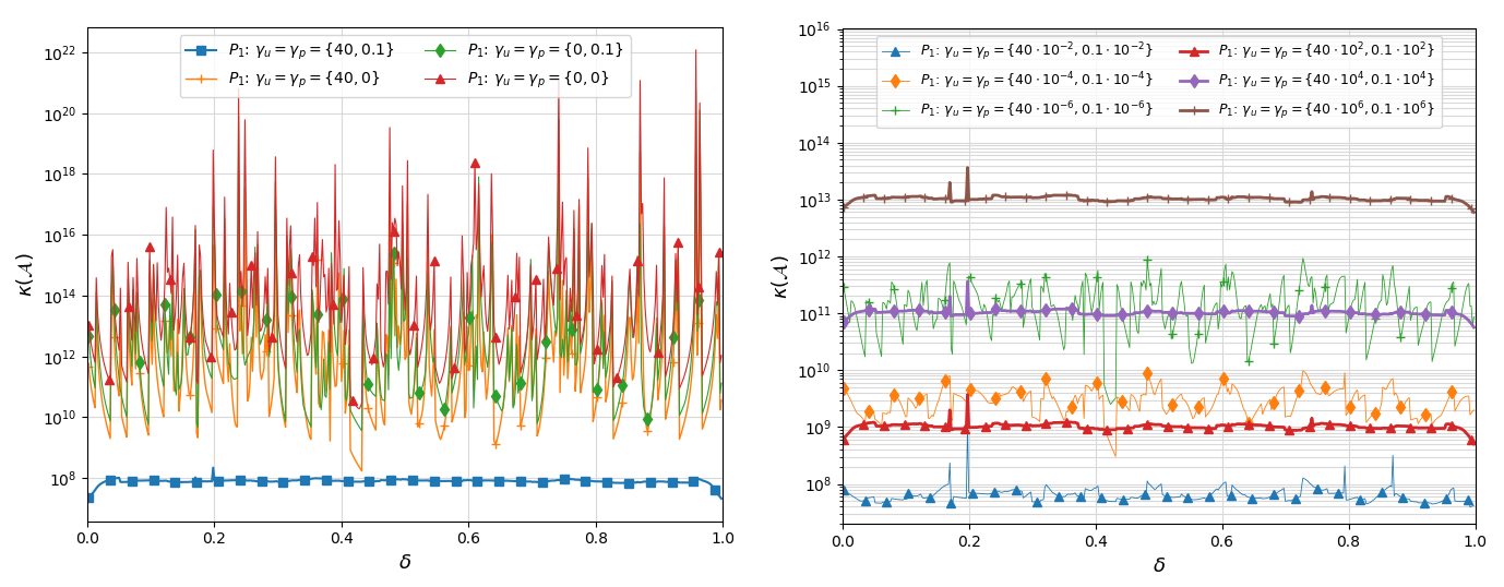
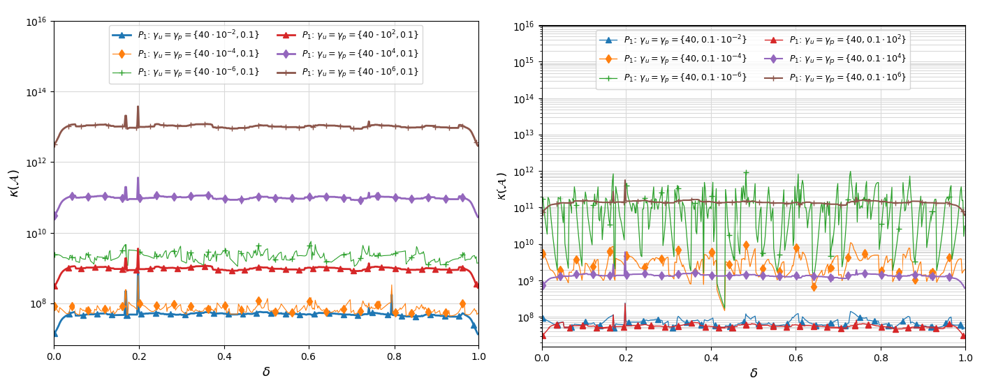
Figure 3. Condition numbers $\kappa(\mathcal{A})$ with respect to parameter $\delta$ for perturbed physical domains $\mathrm{\Omega}_{\delta}=[-0.5+\delta,0.5+\delta]^{2}$ and varying ghost penalty parameters $\gamma_{\mathbf{u}}=\gamma_{p}$. Condition number sensitivity study with and without ghost penalty stabilization (top left) and simultaneously scaled parameters (top right). Condition numbers for a variation of coefficients $\gamma_{0}$ (bottom left) and $\gamma_{1}$ (bottom right). All estimates have been computed using discontinuous $P_{1}-P_{1}$ elements and symmetric interior penalty parameter $\beta=160$.

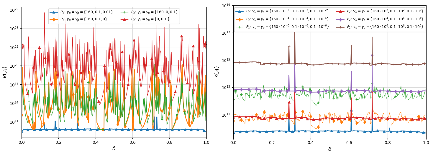
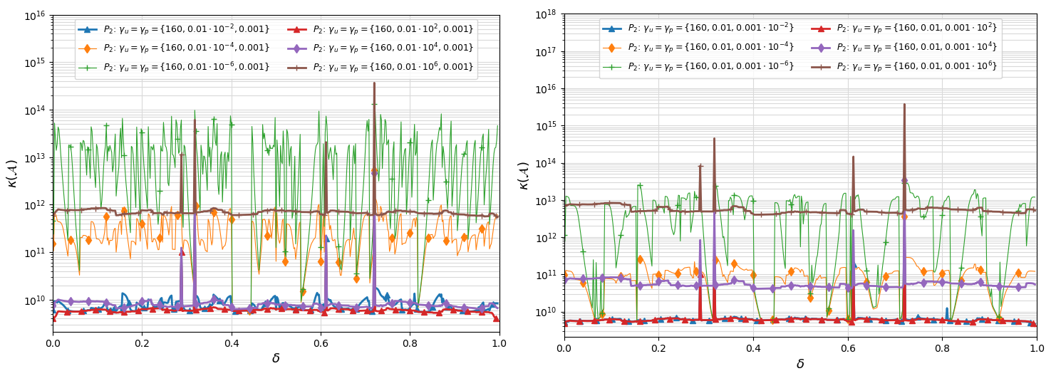
Figure 4. Condition numbers $\kappa(\mathcal{A})$ with respect to parameter $\delta$ for perturbed physical domains $\mathrm{\Omega}_{\delta}=[-0.5+\delta,0.5+\delta]^{2}$ and varying ghost penalty parameters $\gamma_{\mathbf{u}}=\gamma_{p}$. Condition number sensitivity study with and without ghost penalty stabilization (top left) and simultaneously scaled parameters (top right). Condition numbers for a variation of coefficients $\gamma_{1}$ (bottom left), $\gamma_{2}$ (bottom right). All estimates have been computed using discontinuous $P_{2}-P_{2}$ elements and symmetric interior penalty parameter $\beta=1440$.

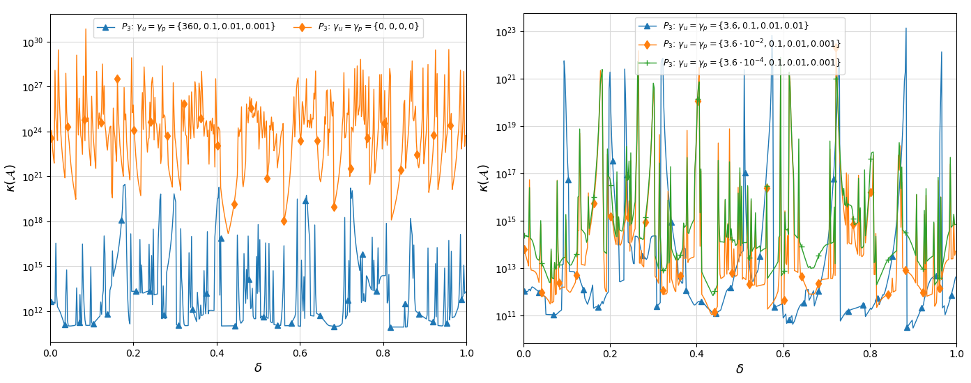
Figure 5. Condition numbers $\kappa(\mathcal{A})$ with respect to parameter $\delta$ for perturbed physical domains $\mathrm{\Omega}_{\delta}=[-0.5+\delta,0.5+\delta]^{2}$ and varying ghost penalty parameters $\gamma_{\mathbf{u}}=\gamma_{p}$. Condition number sensitivity study with and without ghost penalty stabilization (left) and scaled parameter $\gamma_{0}$ (right). All estimates have been computed using discontinuous $P_{3}-P_{3}$ elements and symmetric interior penalty parameter $\beta=1920$.

7.3. Error sensitivity analysis instance for $P_{3}-P_{3}$ finite elements with respect to the cut location

In the current subsection, we focus on the most challenging case of the higher order discontinuous $P_{3}-P_{3}$ finite elements to present the sensitivity of the condition number and the velocity and pressure errors with respect to the cut location. In this experiment, we embed a geometry of smooth boundary representation into a fixed fictitious domain adapting the example of manufactured solution provided in Burman et al [17] to be our exact solution. Let $\mathcal{B}=[-1,1]^{2}$ be the background domain triangulated with mesh size $h=0.05$. We consider the computational domain to be a circular disk centered at the origin. Compatible with the exact solution, velocity field embedded Dirichlet boundary conditions are also weakly imposed.

In order to produce different cut configurations, we uniformly shift the radius of the circle to be $R_{\delta_{\ell}}=R+(\delta_{\ell}+0.04)10^{-2}h$, where $R=0.1$ with respect to a parameter $\delta_{\ell}=2\ell\cdot 10^{-3}$ for $\ell=1,\ldots,250$. Using discontinuous $P_{3}-P_{3}$ finite elements, we estimate the condition number of the associated stiffness matrix and also we measure the $H^{1}$-norm velocity error and the $L^{2}$-norm pressure error for each cut position. We plot the results against the parameter $\delta$ for successively activated ghost penalty parameters at the optimized values from the previous subsection. Representative graphs for the impact of the stabilization term on the condition number and the velocity and pressure errors are shown in Figures 6 and 7, respectively. It is notable that in this test we accomplish robust condition numbers when full ghost penalties are included. It is also clearly visible that absence of the stabilization term results in velocity and pressure errors with large spikes and a strong dependence on the location of the interface, whereas the errors become completely insensitive in case of full ghost penalties. A closer look on the instabilities is also provided and highlighted in the zoomed right plots of Figure 7.

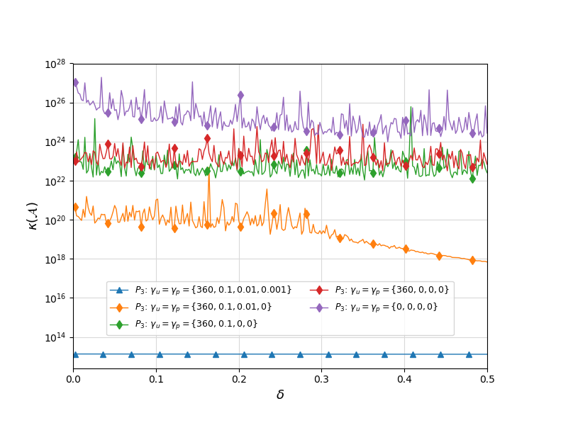
Figure 6. Condition numbers $\kappa(\mathcal{A})$ with respect to parameter $\delta$ for uniformly shifted circular domains of radius $R_{\delta}=0.1+(\delta+0.04)10^{-2}h$ and successively activated ghost penalty parameters $\gamma_{\mathbf{u}}=\gamma_{p}$. The estimates have been computed using discontinuous $P_{3}-P_{3}$ elements.

​​​​​​

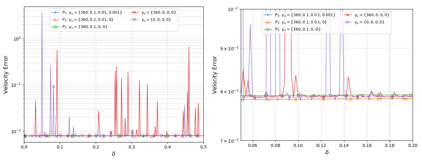
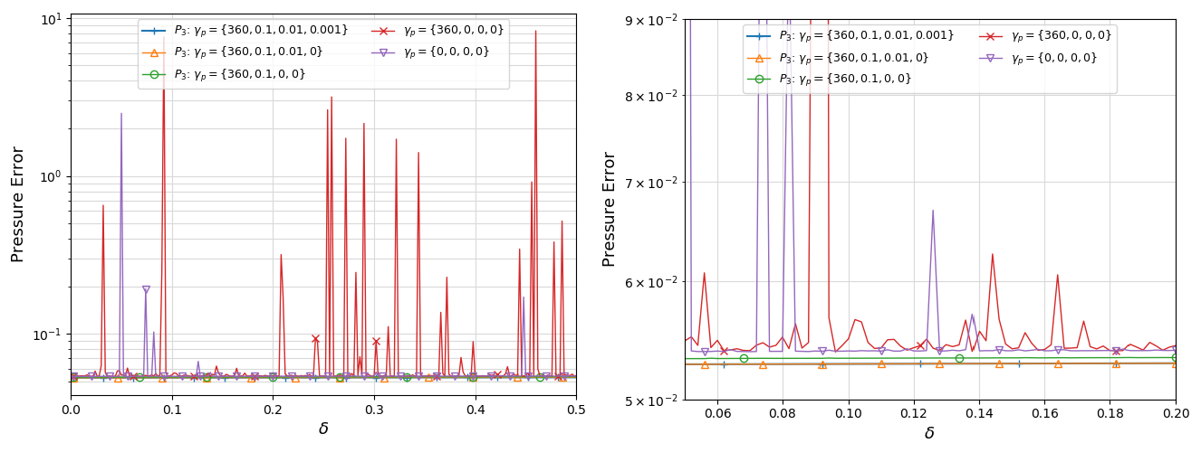
Figure 7. Sensitivities of $H^{1}$-norm velocity errors (top) and $L^{2}$-norm pressure errors (bottom) with respect to parameter $\delta$ for uniformly shifted circular domains of radius $R_{\delta}=0.1+(\delta+0.04)10^{-2}h$ and successively activated ghost penalty parameters $\gamma_{\mathbf{u}}=\gamma_{p}$. A closer look on the error instabilities is highlighted at the right pictures. The estimates have been computed using discontinuous $P_{3}-P_{3}$ elements.

8. Conclusion

In this paper, we proposed and tested a stabilized unfitted discontinuous Galerkin method for the incompressible Stokes flow. Optimal order convergence is proved for higher order finite elements which are discontinuous element-wise polynomials of equal order for both velocity and pressure fields. For this equal order case, pressure face jump penalization is employed to achieve stability in the bulk of the domain. Additionally, to ensure stability and error estimates which are independent of the position of the boundary with respect to the mesh, the formulation is augmented with additional boundary zone ghost penalty terms for both velocity and pressure. These terms act on the jumps of the normal derivatives at faces associated with cut elements. This method may prove valuable in engineering applications where special emphasis is placed on the effective approximation of pressure, attaining much smaller relative errors in coarser meshes. In fact, control over the error of the pressure field is among the most decisive points of difficulty for many methods. Additionally, a uniformly bounded estimate for the condition number $\kappa(\mathcal{A})$ of the stiffness matrix is provided.

Numerical examples demonstrated the stability and accuracy properties of the method. The theoretical convergence rates for the $H^{1}$-norm of the velocity and the $L^{2}$-norm of the pressure have been validated by our tests, even for the $P_{3}-P_{3}$ case. Finally, we employed a condition number sensitivity analysis for a family of perturbed immersed domains with corners in the embedded boundary with respect to several cut configurations and a variation of ghost penalty parameters. In a series of numerical tests for linear and quadratic velocity and pressure approximations, we confirmed the geometrical robustness of the proposed unfitted dG scheme ensuring a well-conditioned system independent of the location of the interface. However, cubic approximations exhibited condition number oscillations with respect to the cut boundary, their magnitudes though lying in a bounded region of values as expected by the respective theory. On the other hand, additional tests on perturbed immersed domains with smooth boundary representation revealed robust condition numbers and velocity and pressure errors for the $P_{3}-P_{3}$ elements.

In the present work, we focused on the static Stokes problem. Future work will also extend our investigations to more general fluid mechanics problems, including time–dependent problems on complex and/or evolving domains.

References

- [1]
- [2] Adjerid S., Chaabane N., Lin T., Yue P.: An immersed discontinuous finite element method for the Stokes problem with a moving interface, J. Comput. Appl. Math. 362, 540–559 (2019).
- [3] Antonietti, P.F., Giani, S., Houston, P.: -Version composite discontinuous Galerkin methods for elliptic problems on complicated domains, SIAM J. Sci. Comput. 35(3), A1417–A1439 (2013).
- [4] Antonietti P.F., Facciola C.,Russo A., Verani M.: Discontinuous Galerkin approximation of flows in fractured porous media on polytopic grids, in: Tech. Rep., MOX, Dipartimento di Matematica, Politecnico di Milano, 2016.
- [5] Aretaki Aik., Karatzas E.N.: Random geometries for optimal control PDE problems based on fictitious domain FEMS and cut elements, accepted for publication, Journal of Computational and Applied Mathematics, 2022, arXiv preprint: https://arxiv.org/pdf/2003.00352.pdf.
- [6] Arnold D.: An interior penalty finite element method with discontinuous elements, SIAM J. Num. Anal. 19(4), 742-760 (1982).
- [7] Barth T., Bochev P., Gunzburger M., Sadid J.: A taxonomy of consistently stabilized methods for the Stokes problem, SIAM J. Numer. Anal. 25(5), 1585-1607 (2004).
- [8] Baker A., Jureidini W.N., Karakashian O.A.: Piecewise solenoidal vector fields and the Stokes problem, SIAM J. Numer. Anal. 27, 1466-1485 (1990).
- [9] Bastian P., Engwer C.: An unfitted finite element method using discontinuous Galerkin, Int. J. Numer. Meth. Engrg. 79, 1557-1576 (2009).
- [10] Bastian P., Engwer C., Fahlke J., Ippisch O.: An unfitted discontinuous Galerkin method for pore–scale simulations of solute transport, Math. Comput. Simulat. 81, 2051-2061 (2011).
- [11] Becker R., Burman E., Hansbo P.: A Nitsche extended finite element method for incompressible elasticity with discontinuous modulus of elasticity. Comput. Methods Appl. Mech. Engrg. 198(41-44), 3352-3360 (2009).
- [12] Bo W., Grove J.W.: A volume of fluid method based ghost fluid method for compressible multi-fluid flows, Computers & Fluids 90, 113-122 (2014).
- [13] Bordas S.P.A., Burman E., Larson M.G., Olshanskii M.A.: Geometrically unfitted finite element methods and applications, Proceedings of the UCL Workshop 2016, Lecture Notes in Computational and Engineering, Springer, 2017.
- [14] Bonito A, Burman E.: A face penalty method for the three fields Stokes equation arising from Oldroyd-B viscoelastic flows, Numer. Math. Adv. Appl. 2, 1–8 (2006).
- [15] Bonito A, Burman E.: A continuous interior penalty method for viscoelastic flows, SIAM J. Sci. Comput. 30, 1156–1177 (2008).
- [16] Burman E., Claus S., Hansbo P., Larson M.G., Massing A.: CutFEM: discretizing geometry and partial differential equations, Int. J. Numer. Meth. Engrg. 104, 472-501 (2014).
- [17] Burman E., Claus S., Massing A.: A stabilized cut finite element method for the three field Stokes problem. SIAM J. Sci. Comput. 37(4), A1705-A1726 (2015).
- [18] Burman E., Delay G., Ern A.: An unfitted hybrid high-order method for the Stokes interface problem. IMA Journal of Numerical Analysis. https://doi.org/10.1093/imanum/draa059 (2020).
- [19] Burman E., Fernández M.A., Hansbo P.: Continuous interior penalty finite element method for Oseen’s equations, SIAM J. Numer. Anal. 44(3), 1248–127 (2006).
- [20] Burman E., Hansbo P.: Fictitious domain finite element methods using cut elements: I. A stabilized Lagrange multiplier method, Comput. Methods Appl. Mech. Engrg. 199(41-44), 2680-2686 (2010).
- [21] Burman E., Hansbo P.: Fictitious domain finite element methods using cut elements II. A stabilized Nitsche method, Appl. Num. Math. 62(4), 328-341 (2012).
- [22] Burman E., Hansbo P.: Fictitious domain methods using cut elements: III. A stabilized Nitsche method for Stokes problem, ESAIM: Math. Model. Numer. Anal. 48(3), 859-874 (2014).
- [23] Burman E., Hansbo P., Larson M.G., Massing A: Cut finite element methods for Partial Differential Equations on embedded manifolds of arbitrary codimensions, ESAIM: M2AN, 52(6), 2247-2282 (2018).
- [24] Burman E., Hansbo P., Larson M.G., Massing A: A cut discontinuous Galerkin method for the Laplace-Beltrami operator, IMA J. Numer. Anal. 37, 138-169 (2017).
- [25] Burman E., Hansbo P., Larson M.G., Massing A., Zahedi S.: A stabilized cut streamline diffusion finite element method for convection-diffusion problems on surfaces, Comput. Methods Appl. Mech. Eng. 358, 11264 (2020).
- [26] Burman E., Hansbo P., Larson M.G., Zahedi S.: Stabilized CutFEM for the convection problem on surfaces, Numer. Math. 141, 103–139 (2019).
- [27] Burman E., Stamm B.: Low order discontinuous Galerkin methods for second-order elliptic problems, SIAM Journal on Numerical Analysis 47, 508–533 (2008).
- [28] Burman E., Stamm B.: Bubble stabilized discontinuous Galerkin method for Stokes problem, Mathematical Models and Methods in Applied Science 20, 297–313 (2010).
- [29] Cangiani A., Dong Z., Georgoulis E.H., Houston P.: Version discontinuous Galerkin methods on polygonal and polyhedral meshes, Springer Briefs in Mathematics (2017).
- [30] Carrero J., Cockburn B., Schotzau D.: Hybridized globally divergence-free LDG methods. part I: The Stokes problem, Math. Comput., 75, 533–563 (2006).
- [31] Cockburn B., Gopalakrishnan J.: Incompressible finite elements via hybridization. Part I the Stokes system in two space dimensions, SIAM J. Numer. Anal. 43(4), 1627–1650 (2005).
- [32] Cockburn B., Kanschat G. , Schötzau D., Schwab C.: Local discontinuous Galerkin methods for the Stokes system, SIAM J. Numer. Anal. 40, 319-343 (2002).
- [33] Cockburn B., Kanschat G., Schötzau D.: An equal-order DG method for the incompressible Navier-Stokes equations, J Sci Comput 40, 188–210 (2009).
- [34] Cockburn B, Kanschat G, Schotzau D.: A note on discontinuous Galerkin divergence-free solutions of the Navier-Stokes equations, J. Sci. Comput. 31(1-2), 61-73 (2007).
- [35] Di Pietro D.A., Ern A.: Mathematical aspects of discontinuous Galerkin methods, volume 69, Springer (2012).
- [36] Dong H., Wang B., Xie Z., Wang L.: An unfitted hybridizable discontinuous Galerkin method for the Poisson interface problem and its error analysis, IMA J. Numer. Anal. 37, 444-476 (2016).
- [37] Duprez M., Lozinski A.: –FEM: a finite element method on domains defined by level–sets, ArXiv: 1901.03966v3, 2019.
- [38] Engwer C., Kuttanikkad S.P.: An unfitted discontinuous Galerkin finite element method for pore scale simulations, PARA 2008, 9th International Workshop on State–of–the–Art in Scientific and Parallel Computing, NTNU, Trondheim, Norway.
- [39] Engwer C., May S., Nüßing A., Streitbürger F.: A stabilized dG cut cell method for the linear transport equation, ArXiv: 1906.05642v1, 2019.
- [40] Engwer C., Ranner T., Westerheide S.: An unfitted discontinuous Galerkin scheme for conservation laws on evolving surfaces, ArXiv: 1602.01080v1, 2016.
- [41] Giani S., Houston P.: Goal-oriented adaptive composite discontinuous Galerkin methods for incompressible flows, J. Comput. Appl. Math. 270, 32–42 (2014).
- [42] Girault V., Rivière B., Wheeler M.: A discontinuous Galerkin method with non–overlapping domain decomposition for the Stokes and Navier–Stokes problems, Math. Comput. 74, 53-84 (2005).
- [43] Groß S., Reusken A.: An extended pressure finite element space for two-phase incompressible flows with surface tension, J. Comput. Phys. 224 no. 1, 40–58 (2007).
- [44] Gürkan C., Krombichler M., Fernández-Méndez S.: Extended hybridizable discontinuous Galerkin method for incompressible flow problems with unfitted meshes and interfaces, Int. J. Numer. Meth. Engrg. 117, 756-777 (2019).
- [45] Gürkan C., Massing A.: A stabilized cut discontinuous Galerkin framework for elliptic boundary value and interface problems, Comput. Methods Appl. Mech. Eng. 348, 466-499 (2019).
- [46] Gürkan C., Sticko S., Massing A.: Stabilized cut discontinuous Galerkin methods for advection-reaction problems, SIAM Journal on Scientific Computing 42(5), A2620-A2654 (2020).
- [47] Guzmán, J., Olshanskii, M.A.: Inf-sup stability of geometrically unfitted Stokes finite elements, Math. Comp. 87, 2091-2112 (2018).
- [48] Hansbo P.: Nitsche’s method for interface problems in computational mechanics, GAMM-Mitteilungen 28(2), 183-206 (2005).
- [49] Hansbo A., Hansbo P.: An unfitted finite element method, based on Nitsche’s method, for elliptic interface problems, Comput. Methods Appl. Mech. Eng. 191, 5537-5552 (2002).
- [50] Hansbo A., Hansbo P., Larson M.G.: A finite element method on composite grids based on Nitsche’s method, ESAIM: Math. Model. Numer. Anal. 37, 495-514 (2003).
- [51] Hansbo P., Larson M.G.: Discontinuous Galerkin methods for incompressible and nearly incompressible elasticity by Nitsche’s method. Computer Methods in Applied Mechanics and Engng, 191, 1895–1908 (2002).
- [52] Hansbo P., Larson M.G., Zahedi S.: A cut finite element method for a Stokes interface problem, Applied Numerical Mathematics 85, 90-114 (2014).
- [53] Heimann F., Engwer C, Ippisch O., Bastian P.: An unfitted interior penalty discontinuous Galerkin method for incompressible Navier–Stokes two–phase flow, Internat. J. Numer. Methods Fluids 71, 269–293 (2013).
- [54] Huynh L.N.T., Nguyen N.C., Peraire J., Khoo B.C.: A high order hybrizidable discontinuous Galerkin method for elliptic interface problems, Int. J. Numer. Meth. Engrg. 93, 183-200 (2013).
- [55] Johansson A., Larson M.G.: A high order discontinuous Galerkin Nitsche method for elliptic problems with fictitious boundary, Numer. Math. 123(4), 607-628 (2013).
- [56] Johansson A., Larson M.G., Logg A.: High order cut finite element methods for the Stokes system, Adv. Model. and Simul. in Eng. Sci. 2(24), 2-24 (2015).
- [57] Karatzas E.N., Ballarin F., Rozza G.: Projection-based reduced order models for a cut finite element method in parametrized domains, Computers & Mathematics with Applications 79, no. 3, 833-851 (2020).
- [58] Karatzas E.N., Stabile G., Atallah N., Scovazzi G., Rozza G.: A reduced order approach for the embedded shifted boundary FEM and a heat exchange system on parametrized geometries, In: Fehr J., Haasdonk B. (eds) IUTAM Symposium on Model Order Reduction of Coupled Systems, Stuttgart, Germany, May 22-25, 2018. IUTAM Bookseries, vol 36. Springer, Cham (2020).
- [59] Karatzas E.N., Stabile G., Nouveau L., Scovazzi G., Rozza G.: A reduced basis approach for PDEs on parametrized geometries based on the shifted boundary finite element method and application to a Stokes flow, Comput. Methods Appl. Mech. Engrg. 347, 568-587 (2019).
- [60] Karatzas E.N., Stabile G., Nouveau L., Scovazzi G., Rozza G.: A reduced-order shifted boundary method for parametrized incompressible Navier-Stokes equations, Comput. Methods Appl. Mech. Engrg. 370, 113-273 (2020).
- [61] Karakashian O. A., Jureidini W. N.: A nonconforming finite element method for the stationary Navier-Stokes equations, SIAM J. Numer. Anal., 35(1), 93–120 (1998).
- [62] Katsouleas G., Karatzas E.N., Travlopanos F.: Cut finite element error estimates for a class of nonlinear elliptic PDEs, Loughborough University, doi: https://doi.org/10.17028/rd.lboro.12154854.v1, extended version at arXiv:2003.06489 (2020).
- [63] Kirchhart M., Groß S., Reusken A.: Analysis of an XFEM discretization for Stokes interface problems, SIAM J.Sci.Comput. 38(2), A1019–A1043 (2016).
- [64] Krause D., Kummer F.: An incompressible immersed boundary solver for moving body flows using a cut cell discontinuous Galerkin method, Comput. Fluids 153, 118-129 (2017).
- [65] Kummer F.: Extended discontinuous galerkin methods for two-phase flows: the spatial discretization, Internat. J. Numer. Meth. Engrg, 109, 259–289 (2017).
- [66] Lederer P., Pfeiler C.M., Wintersteiger C., Lehrenfeld C.: Higher order unfitted FEM for Stokes interface problems, Proc. Applied Math. and Mech 16(1), 7-10 (2016).
- [67] Lehrenfeld C.: High order unfitted finite element methods on level set domains using isoparametric mappings, Comput. Methods Appl. Mech. Engrg. 300, 716-733 (2016).
- [68] Kolahdouz E.M., Bhalla A.P.S., Craven B.A., Griffith B.E.: An immersed interface method for faceted surfaces, Journal of Computational Physics, 400 (2020).
- [69] Lehrenfeld C. , Heimann F., Preuß J. and von Wahl H.: ngsxfem: Add-on to NGSolve for geometrically unfitted finite element discretizations, Journal of Open Source Software, 6(64), 3237, https://doi.org/10.21105/joss.03237.
- [70] Li R., Sun Z., Yang F., Yang Z.: A finite element method with path reconstruction for the Stokes problem using mixed formulations, J. Comput. Appl. Math. 353, 1-20 (2018).
- [71] Lozinski A.: CutFEM without cutting the mesh cells: a new way to impose Dirichlet and Neumann boundary conditions on unfitted meshes, Computer Methods in Applied Mechanics and Engineering, 356, 75-100 (2019).
- [72] Luo H., Luo L., Ali A., Nourgaliev R., Cai C.: A parallel, reconstructed Discontinuous Galerkin method for the compressible flows on arbitrary grids, Commun. Comput. Phys., 9(2), 363-389 (2011).
- [73] Main A., Scovazzi G.: The shifted boundary method for embedded domain computations. Part I: Poisson and Stokes problems, J. Comput. Phys. 372, 972-995 (2018).
- [74] Massjung R.: An unfitted discontinuous Galerkin method applied to elliptic interface problems, SIAM J. Numer. Anal. 50, 3134-3162 (2012).
- [75] Massing A.: A cut discontinuous Galerkin method for coupled bulk-surface problems, Chapter in UCL Workshop volume on “Geometrically Unfitted Finite Element Methods”, Lecture Notes in Computational Science and Engineering, Springer, 259–279, 2017.
- [76] Massing A., Larson M.G., Logg A., Rognes M.E.: A stabilized Nitsche fictitious domain method for the Stokes problem, J. Sci. Comput. 61, 604-628 (2014).
- [77] Massing A., Larson M.G., Logg A., Rognes M.E.: A stabilized Nitsche overlapping mesh method for the Stokes problem, Numer. Math. 128, 73-101 (2014).
- [78] Massing A., Schott B., Wall W.: A stabilized Nitsche cut finite element method for the Oseen problem, Comput. Methods Appl. Mech. Engrg. 328, 262–300 (2018).
- [79] Mittal R., and Iaccarino G.: Immersed boundary methods, Annual Review of Fluid Mechanics 37(1), 239-261 (2005).
- [80] Montlaur, A., Fernandez‐Mendez, S., Huerta, A.: Discontinuous Galerkin methods for the Stokes equations using divergence‐free approximations, Int. J. Numer. Meth. Fluids 57, 1071-1092 (2008).
- [81] Müller B., Krämer-Eis S., Kummer F., Oberlack M.: A high-order Discontinuous Galerkin method for compressible flows with immersed boundaries, Int. J. Numer. Methods Eng. 110, 3-30 (2017).
- [82] Nüßing A., Wolters C.H., Brinck H., Engwer C.: The unfitted discontinuous Galerkin method for solving the EEG forward problem, IEEE Transactions in Biomedical Engineering 63, 2564-2575 (2016).
- [83] Quarteroni A.: Numerical models for differential problems. Modeling, simulation and applications, Springer, Berlin (2009).
- [84] Pasquariello V., Hammerl G., Órley F., Hickel S., Danowski C., Popp A., Wall W.A., Adams N.A.: A cut-cell finite volume–finite element coupling approach for fluid–structure interaction in compressible flow, J. Comput. Phys. 307, 670-695 (2016).
- [85] Peskin C.S.: Flow patterns around heart valves: A numerical method, J. Comput. Phys. 10, 252-271 (1972).
- [86] Saye R.: Implicit mesh discontinuous Galerkin methods and interfacial gauge methods for high-order accurate interface dynamics, with applications to surface tension dynamics, rigid body fluid-structure interaction, and free surface flow: Part I, J. Comput. Phys. 344, 647-682 (2017).
- [87] Saye R.: Implicit mesh discontinuous Galerkin methods and interfacial gauge methods for high-order accurate interface dynamics, with applications to surface tension dynamics, rigid body fluid–structure interaction, and free surface flow: Part II, J. Comput. Phys. 344, 683–723 (2017).
- [88] Saye, R.I.: High-order quadrature methods for implicitly defined surfaces and volumes in hyperrectangles, SIAM J. Sci. Comput. 37(2), A993–A1019 (2015).
- [89] Schötzau D., Schwab C., Toselli A.: Mixed hp-DGFEM for incompressible flows, SIAM J. Numer. Anal. 40, 2171-2194 (2003).
- [90] Schöberl, J. : C++11 Implementation of Finite Elements in NGSolve, ASC Report 30/2014, Institute for Analysis and Scientific Computing, Vienna University of Technology, (2014).
- [91] B. Schott B., Wall W.A.: A new face-oriented stabilized XFEM approach for 2D and 3D incompressible Navier–Stokes equations, Comput. Methods Appl. Mech. Engrg. 276, 233–265 (2014).
- [92] Sollie W.E.H., Bokhove O., Van der Vegt J.J.W.: Space–time discontinuous Galerkin finite element method for two-fluid flows, J. Comput. Phys. 230(3), 789–817 (2011).
- [93] Sonntag M.,Munz, C.D.: Efficient parallelization of a shock capturing for discontinuous Galerkin methods using finite volume sub-cells. Journal of Scientific Computing 70(3), 1262–1289 (2017).
- [94] Toselli A.: HP-discontinuous Galerkin approximations for the Stokes problem, Mathematical Models and Methods in Applied Sciences 12(11), 1565-1597 (2002).
- [95] Wang Q., Chen J.: Unfitted discontinuous Galerkin method for elliptic interface problems, Journal of Applied Mathematics 13(3), 1-10 (2014).
- [96] Winter M., Schott B., Massing A., Wall W.: A Nitsche cut finite element method for the Oseen problem with general Navier boundary conditions, Comput. Methods Appl. Mech. Engrg. 330, 220–252 (2017).
- [97] Wu C.H., Faltinsen O.M., Chen B.F.: Time-independent finite difference and ghost cell method to study sloshing liquid in 2D and 3D tanks with internal structures, Comm. Comput. Phys. 13(3), 780-800 (2013).
- [98] ngsxfem - Add-On to NGSolve for unfitted finite element discretizations, https://github.com/ngsxfem/ngsxfem, 2020.
- [99] NGSolve - high performance multiphysics finite element software, https://github.com/NGSolve/ngsolve, 2020.