Microscopic pairing theory of a binary Bose mixture with interspecies attractions: bosonic BEC-BCS crossover and ultradilute low-dimensional quantum droplets

Abstract

Ultradilute quantum droplets are intriguing new state of matter, in which the attractive mean-field force can be balanced by the repulsive force from quantum fluctuations to avoid collapse. Here, we present a microscopic theory of ultradilute quantum droplets in three-, one- and two-dimensional two-component Bose-Bose mixtures, by generalizing the conventional Bogoliubov theory to include the bosonic pairing arising from the interspecies attraction. Our pairing theory is fully equivalent to a variational approach and hence gives an upper bound for the energy of quantum droplets. In three dimensions, we predict the existence of a strongly interacting Bose droplet at the crossover from Bose-Einstein condensates (BEC) to Bardeen–Cooper–Schrieffer (BCS) superfluids and map out the bosonic BEC-BCS crossover phase diagram. In one dimension, we find that the energy of the one-dimensional Bose droplet calculated by the pairing theory is in an excellent agreement with the latest diffusion Monte Carlo simulation [Phys. Rev. Lett. 122, 105302 (2019)], for nearly all the interaction strengths at which quantum droplets exist. In two dimensions, we show that Bose droplets disappear and may turn into a soliton-like many-body bound state, when the interspecies attraction exceeds a critical value. Below the threshold, the pairing theory predicts more or less the same results as the Bogoliubov theory derived by Petrov and Astrakharchik [Phys. Rev. Lett. 117, 100401 (2016)]. The predicted energies from both theories are higher than the diffusion Monte Carlo results, due to the weak interspecies attraction and the increasingly important role played by the beyond-Bogoliubov-approximation effect in two dimensions. Our pairing theory provides an ideal starting point to understand interesting ground-state properties of quantum droplets in various dimensions, including their shape and collective oscillations.

I Introduction

In the weakly interacting regime, quantum phase of ultracold atomic Bose gases is typically determined by their mean-field interactions (Dalfovo1999, ). Attractive mean-field interactions can induce mechanical instability towards collapse (Donley2001, ). This common viewpoint, however, is radically changed due to the seminal work by Petrov (Petrov2015, ), who proposed that the mean-field collapse could be prevented by the repulsive force provided by quantum fluctuations, i.e., the celebrated Lee-Huang-Yang (LHY) correction to the energy functional (LeeHuangYang1957, ). Although the beyond-mean-field LHY correction is usually small, it can be made comparable to the mean-field energy by experimentally tuning the interatomic interactions with the Feshbach resonance technique. As a result, self-bound liquid-like quantum droplets may form, even in free space without container (Petrov2018, ; FerrierBarbut2019, ; Kartashov2019, ). Petrov’s ground-breaking proposal has now been surprisingly confirmed in single-component Bose gases with anisotropic dipolar forces (FerrierBarbut2016, ; Schmitt2016, ; Chomaz2016, ; Bottcher2019PRA, ; Bottcher2019PRX, ) and in two-component Bose-Bose mixtures with contact inter-particle interactions (Cabrera2018, ; Cheiney2018, ; Semeghini2018, ; Ferioli2019, ; DErrico2019, ). It opens a new rapidly developing research field (Bottcher2020, ), where the beyond-mean-field many-body effect could be systematically explored, both experimentally (FerrierBarbut2016, ; Schmitt2016, ; Chomaz2016, ; Bottcher2019PRA, ; Bottcher2019PRX, ; Cabrera2018, ; Cheiney2018, ; Semeghini2018, ; Ferioli2019, ; DErrico2019, ) and theoretically (Petrov2016, ; Baillie2016, ; Wachtler2016, ; Baillie2017, ; Li2017, ; Cappellaro2017, ; Jorgensen2018, ; Cui2018, ; Staudinger2018, ; Parisi2019, ; Cikojevic2019, ; Tylutki2020, ; Shi2019, ; Cikojevic2020, ; Wang2020, ; Hu2020a, ; Ota2020, ).

Despite the great success of Petrov’s proposal, strictly speaking, it is not a consistent microscopic theory. This is particularly clear for three-dimensional Bose-Bose mixtures, with which the Petrov prototype theory of quantum droplets was constructed, within the Bogoliubov approximation (Petrov2015, ; Larsen1963, ). As the mean-field solution is not stable towards collapse, one of the two gapless Bogoliubov modes becomes softened and acquires a small imaginary component. This results in a complex LHY energy functional (Petrov2015, ; Cikojevic2019, ; Hu2020a, ; Ota2020, ), which is not physical. To circumvent this technical issue, Petrov assumed a weak dependence of the LHY energy functional on the interspecies interaction strength and fixed the LHY energy to the value on the verge of the collapse where the mechanical instability first sets in (Petrov2015, ). Hereafter, we will refer to such an approximation as Petrov’s prescription. Due to the intrinsic inconsistency in the Petrov prototype theory, the resulting energy of quantum droplets shows an appreciable deviation from the numerically accurate diffusion Monte Carlo (DMC) predictions (Cikojevic2019, ). The predicted critical number for the droplet formation also seems to be larger than the one measured experimentally, both in dipolar Bose gases (Bottcher2019PRA, ) and in Bose-Bose mixtures (Cabrera2018, ).

Recently, we developed a consistent microscopic theory to remove the annoying loophole in the Petrov theory of quantum droplets (Hu2020a, ). The crucial ingredient of the theory is the inclusion of a weak bosonic pairing between different components due to the attractive interspecies interactions. The pairing explicitly removes the unstable softened Bogoliubov excitation and turns it into a stable gapped mode, as in the conventional Bardeen-Cooper-Schrieffer (BCS) theory for interacting fermions (BCS1957, ). An apparent advantage of the pairing theory is that, it is variational and therefore predicts an upper bound for the ground-state energy. Remarkably, in three dimensions our pairing theory leads to an improved agreement with the DMC simulation, for the energy and the equilibrium density of quantum droplets (Hu2020a, ).

In this work, we would like to provide more details of the microscopic pairing theory in three dimensions (Hu2020a, ), on the equation derivation and the numerical calculation. In particular, we show that the weakly interacting pairing in our previous study can be naturally generalized to the strongly interacting regime, in which the interspecies scattering length diverges across a Feshbach resonance. Therefore, we predict the existence of a strongly interacting Bose droplet, where a significant fraction of atoms turns into bound pairs. This is precisely analogous to the crossover physics from a Bose-Einstein condensate (BEC) to a BCS superfluid (NSR1985, ; Hu2006, ; Diener2008, ), recently observed with fermionic ⁴⁰K and ⁶Li atoms (Regal2004, ; Zwierlein2004, ). Across the bosonic BEC-BCS crossover, the interspecies scattering length becomes positive and small, and the strongly interacting Bose droplet eventually disappears and turns into a gas of tightly-bound molecules or dimers via a first-order phase transition.

We then focus on the new cases of low-dimensional quantum droplets and examine systematically their bulk properties. Our pairing theory turns out to work extremely well in one dimension. For nearly all the interaction strengths at which quantum droplets exist, we find an excellent agreement between the theory and the DMC simulation for the ground-state energy (Parisi2019, ). In two dimensions, quantum droplets emerges for an arbitrarily weak interspecies interaction strength. Due to the weakness of the interspecies attraction, our pairing theory does not differ too much with the Petrov theory (Petrov2016, ). Both theories fail to have a good agreement with the DMC simulation, presumably due to the beyond-LHY-correction that becomes increasingly important in two dimensions (Mora2009, ; Astrakharchik2009, ). Nevertheless, it is remarkable that with increasing interspecies attraction our pairing theory predict a critical attraction, above which quantum droplets cease to exist. This critical value is consistent with the threshold for zero-crossing in dimer-dimer scatterings from a four-body problem in two dimensions (Guijarro2020, ). Above the threshold, the effective interaction between dimers (i.e., tightly bound bosonic pairs) changes from weakly attractive to weakly repulsive, indicating the instability of quantum droplets in the few-body limit.

The rest of the paper is organized as follows. In the next section (Sec. II), we introduce the model Hamiltonian for two-component Bose-Bose mixtures and present the pairing theory, i.e, the Bogoliubov theory with bosonic pairing. We mention briefly the concept of a bosonic BEC-BCS crossover. In Sec. III, the connection of our pairing theory to the conventional Bogoliubov theory without pairing is discussed. In Sec. IV, Sec. V, and Sec. VI, we consider the three-, one-, and two-dimensional cases, respectively. In three dimensions, we show the existence of a strongly interacting Bose droplet and map out the phase diagram of the bosonic BEC-BCS crossover. In the low-dimensional cases, we discuss in detail the comparison of the pairing theory to the benchmark DMC simulations and the physics near the threshold, at which the Bose droplet starts to disappear. Finally, Sec. VII is devoted to conclusions and outlooks.

II The model Hamiltonian and pairing theory

We consider a two-component Bose-Bose mixture as in the seminal work by Petrov (Petrov2015, ). To be specific, let us focus on homonuclear mixtures such as the ³⁹K-³⁹K mixture, with which the masses of the two components are the same, i.e., $m_{1}=m_{2}=m$. In the presence of the intraspecies interactions $g_{11}$ and $g_{22}$, and the interspecies interactions $g_{12}=g_{21}$, the system in free space can be described the following Hamiltonian density,

$$\mathscr{H}\left(\mathbf{x}\right) = \mathscr{H}_{0}\left(\mathbf{x}\right)+\mathscr{H}_{\textrm{int}}\left(\mathbf{x}\right),$$ (1)

$$\mathscr{H}_{0}\left(\mathbf{x}\right) = \sum_{i=1,2}\phi_{i}^{\dagger}\left(\mathbf{x}\right)\left[-\frac{\hbar^{2}\nabla^{2}}{2m}-\mu_{i}\right]\phi_{i}\left(\mathbf{x}\right),$$ (2)

$$\mathscr{H}_{\textrm{int}}\left(\mathbf{x}\right) = \sum_{i,j=1,2}\frac{g_{ij}}{2}\phi_{i}^{\dagger}\left(\mathbf{x}\right)\phi_{j}^{\dagger}\left(\mathbf{x}\right)\phi_{j}\left(\mathbf{x}\right)\phi_{i}\left(\mathbf{x}\right),$$ (3)

where $\phi_{i}(\mathbf{x})$ ($i=1,2$) is the annihilation field operator of the $i$-species bosons and $\mu_{i}$ is the chemical potential. In three or two dimensions, the use of contact inter-particle interactions leads to the well-known ultraviolet divergence, so the bare interaction strengths $g_{ij}$ need regularization and are to be replaced by the $s$-wave scattering lengths $a_{ij}$ or the binding energies $E_{B}^{ij}$. For example, in three dimensions we may write,

$$\frac{1}{g_{ij}}=\frac{m}{4\pi\hbar^{2}a_{ij}}-\frac{1}{\mathcal{V}}\sum_{k}\frac{m}{\hbar^{2}\mathbf{k}^{2}},$$ (4)

where the volume $\mathcal{V}$ (or area in two dimensions and length in one dimension) will be set to unity hereafter.

We use the conventional path-integral formalism to describe our bosonic pairing theory, following its fermionic counterpart (He2015, ; Hu2020b, ). We are interested in calculating the thermodynamic potential $\varOmega$ from the partition function,

$$\mathcal{Z}=\int\mathcal{D}[\phi_{1},\phi_{2}]e^{-\mathcal{S}},$$ (5)

where the action is given by,

$$\mathcal{S}=\int dx\left[\sum_{i=1,2}\bar{\phi}_{i}\left(x\right)\partial_{\tau}\phi_{i}\left(x\right)+\mathscr{H}\left(x\right)\right].$$ (6)

Here, we have used the standard notations $x\equiv(\mathbf{x},\tau)$ and $\int dx\equiv\int d\mathbf{x}\int_{0}^{\beta}d\tau$, and $\beta\equiv 1/(k_{B}T)$.

Due to the attractive interspecies interaction (i.e, $g_{12}<0$), we anticipate the pairing between different species. To make it evident, we explicitly introduce an auxiliary pairing field $\Delta(x)$ and take the Hubbard–Stratonovich transformation to decouple the Hamiltonian density for interspecies interactions, i.e.,

$$\exp\left[-g_{12}\int dx\bar{\phi}_{1}\bar{\phi}_{2}\phi_{2}\phi_{1}\right]=\int\mathcal{D}\left[\Delta\left(x\right)\right]\exp\left\{\int dx\left[\frac{\left|\Delta\left(x\right)\right|^{2}}{g_{12}}+\left(\bar{\Delta}\phi_{2}\phi_{1}+\bar{\phi}_{1}\bar{\phi}_{2}\Delta\right)\right]\right\}.$$ (7)

The action then becomes,

$$\mathcal{S}=\int dx\left[-\frac{\left|\Delta\left(x\right)\right|^{2}}{g_{12}}-\left(\bar{\Delta}\phi_{2}\phi_{1}+\bar{\phi}_{1}\bar{\phi}_{2}\Delta\right)\right]+\sum_{i=1,2}\int dx\left[\bar{\phi}_{i}\left(\partial_{\tau}-\frac{\hbar^{2}\nabla^{2}}{2m}-\mu_{i}\right)\phi_{i}+\frac{g_{ii}}{2}\bar{\phi}_{i}^{2}\phi_{i}^{2}\right].$$ (8)

For the pairing field $\Delta(x)$, it suffices to take a uniform saddle-point solution $\Delta(x)=\Delta>0$. At the same level of the Bogoliubov approximation, at zero temperature we assume the bosons condensate into the zero-momentum states, i.e.,

$$\phi_{i}\left(x\right) = \phi_{ic}+\delta\phi_{i}\left(x\right),$$ (9)

with a positive wave-function $\phi_{ic}>0$. Following the Bogoliubov approximation, the intraspecies interaction terms may be approximated as,

$$\frac{g_{ii}}{2}\bar{\phi}_{i}^{2}\phi_{i}^{2}\simeq\frac{C_{i}^{2}}{2g_{ii}}+\frac{C_{i}}{2}\left(4\delta\bar{\phi}_{i}\delta\phi_{i}+\delta\bar{\phi}_{i}\delta\bar{\phi}_{i}+\delta\phi_{i}\delta\phi_{i}\right),$$ (10)

where $C_{i}=g_{ii}\phi_{ic}^{2}$. As a consequence, we find the effective action $\mathcal{S}\simeq\beta\mathcal{V}\varOmega_{0}+\mathcal{S}_{B}$, where the condensate thermodynamic potential $\varOmega_{0}$ is given by,

$$\varOmega_{0}=\sum_{i=1,2}\left(-\mu_{i}\phi_{ic}^{2}+\frac{C_{i}^{2}}{2g_{ii}}\right)-\frac{\Delta^{2}}{g_{12}}-2\Delta\phi_{1c}\phi_{2c},$$ (11)

and the quantum fluctuations around the condensates have the contribution,

$$\mathcal{S}_{B} =-\int dx\Delta\left(\delta\bar{\phi}_{1}\delta\bar{\phi}_{2}+\delta\phi_{2}\delta\phi_{1}\right)+\int dx\sum_{i=1,2}$$

$$\left[\delta\bar{\phi}_{i}\left(\partial_{\tau}+\hat{B}_{i}\right)\delta\phi_{i}+\frac{C_{i}}{2}\left(\delta\bar{\phi}_{i}\delta\bar{\phi}_{i}+\delta\phi_{i}\delta\phi_{i}\right)\right],$$ (12)

with $\hat{B}_{i}(x)\equiv-\hbar^{2}\nabla^{2}/(2m)-\mu_{i}+2C_{i}$. By introducing a Nambu spinor $\Phi(x)=[\delta\phi_{1}(x),\delta\bar{\phi}_{1}(x),\delta\phi_{2}(x),\delta\bar{\phi}_{2}(x)]^{T}$, we may recast $\mathcal{S}_{B}$ into a compact form,

$$\mathcal{S}_{B}=\int dxdx^{\prime}\bar{\Phi}\left(x\right)\left[-\mathscr{D}^{-1}\left(x,x^{\prime}\right)\right]\Phi\left(x^{\prime}\right),$$ (13)

where the inverse Green function of bosons is given by,

$$\mathscr{D}^{-1}=\left[\begin{array}[]{cccc}-\partial_{\tau}-\hat{B}_{1}&-C_{1}&0&\Delta\\ -C_{1}&\partial_{\tau}-\hat{B}_{1}&\Delta&0\\ 0&\Delta&-\partial_{\tau}-\hat{B}_{2}&-C_{2}\\ \Delta&0&-C_{2}&\partial_{\tau}-\hat{B}_{2}\end{array}\right].$$ (14)

Due to the delta function $\delta\left(x-x^{\prime}\right)$ in $\mathscr{D}^{-1}(x,x^{\prime})$, which we do not explicitly show in the above equation, it is convenient to work in momentum space by performing a Fourier transform. After replacing $-\partial_{\tau}$ with the bosonic Matasubara frequencies $i\omega_{m}$ (i.e., $\omega_{m}=2\pi mk_{B}T$ with $m\subseteq\mathbb{Z}$) and performing the analytic continuation $i\omega_{m}\rightarrow\omega+i0^{+}$, i.e.,

$$-\partial_{\tau}\rightarrow\omega+i0^{+},$$ (15)

and taking the replacement

$$\hat{B}_{i}\rightarrow B_{i\mathbf{k}}=\varepsilon_{\mathbf{k}}-\mu_{i}+2C_{i}$$ (16)

with $\varepsilon_{\mathbf{k}}=\hbar^{2}\mathbf{k}^{2}/(2m)$, it is straightforward to explicitly write down the expression of $\mathscr{D}^{-1}(\mathbf{k},\omega)$. By solving the poles of the bosonic Green function, i.e., $\det[\mathscr{D}^{-1}(\mathbf{k},\omega\rightarrow E(\mathbf{k}))]=0$, or more explicitly,

$$\omega^{4}-\omega^{2}\left[\left(B_{1\mathbf{k}}^{2}-C_{1}^{2}\right)+\left(B_{2\mathbf{k}}^{2}-C_{2}^{2}\right)-2\Delta^{2}\right]+\left[\left(B_{1\mathbf{k}}^{2}-C_{1}^{2}\right)\left(B_{2\mathbf{k}}^{2}-C_{2}^{2}\right)-2\left(B_{1\mathbf{k}}B_{2\mathbf{k}}+C_{1}C_{2}\right)\Delta^{2}+\Delta^{4}\right]=0,$$ (17)

we obtain the two Bogoliubov spectra,

$$E_{\pm}^{2}\left(\mathbf{k}\right)=\left[\mathcal{A}_{+}\left(\mathbf{k}\right)-\Delta^{2}\right]\pm\sqrt{\mathcal{A}_{-}^{2}\left(\mathbf{k}\right)+\Delta^{2}\left[\left(C_{1}+C_{2}\right)^{2}-\left(B_{1\mathbf{k}}-B_{2\mathbf{k}}\right)^{2}\right]},$$ (18)

where we have defined,

$$\mathcal{A}_{\pm}\left(\mathbf{k}\right)=\frac{\left(B_{1\mathbf{k}}^{2}-C_{1}^{2}\right)\pm\left(B_{2\mathbf{k}}^{2}-C_{2}^{2}\right)}{2}.$$ (19)

II.1 Thermodynamic potential

By taking the derivative of the condensate thermodynamic potential $\varOmega_{0}$ in Eq. (11) with respect to $\phi_{1c}$ and $\phi_{2c}$, we find that,

$$-\mu_{1}\phi_{1c}+g_{11}\phi_{1c}^{3}-\Delta\phi_{2c} = 0,$$ (20)

$$-\mu_{2}\phi_{2c}+g_{22}\phi_{2c}^{3}-\Delta\phi_{1c} = 0.$$ (21)

Therefore, we obtain

$$-\mu_{1}+C_{1}=B_{1\mathbf{k}=0}-C_{1} = \Delta\left(\phi_{2c}/\phi_{1c}\right),$$ (22)

$$-\mu_{2}+C_{2}=B_{2\mathbf{k}=0}-C_{2} = \Delta\left(\phi_{1c}/\phi_{2c}\right),$$ (23)

and hence

$$\left(B_{1\mathbf{k}=0}-C_{1}\right)\left(B_{2\mathbf{k}=0}-C_{2}\right)=\Delta^{2}.$$ (24)

As the last term in Eq. (17) can be rewritten as the product of $(B_{1\mathbf{k}}-C_{1})(B_{2\mathbf{k}}-C_{2})-\Delta^{2}$ and $(B_{1\mathbf{k}}+C_{1})(B_{2\mathbf{k}}+C_{2})-\Delta^{2}$, the term is zero at zero momentum $\mathbf{k}=0$. Thus, we confirm that at least one of the two Bogoliubov spectra is gapless. This is anticipated from the $U(1)$ symmetry breaking of the system. On the other hand, it is straightforward to rewrite the condensate thermodynamic potential in the form,

$$\varOmega_{0}=-\frac{\Delta^{2}}{g_{12}}-\frac{C_{1}^{2}}{2g_{11}}-\frac{C_{2}^{2}}{2g_{22}}.$$ (25)

We now turn to consider the action for quantum fluctuations $\mathcal{S}_{B}$, which gives the LHY contribution to the thermodynamic potential (Salasnich2016, ; Hu2020c, ),

$$\varOmega_{\textrm{LHY}} =\frac{k_{B}T}{2}\sum_{\mathbf{q},i\omega_{m}}\ln\det\left[\mathscr{-D}^{-1}\left(\mathbf{q},i\omega_{m}\right)\right]e^{i\omega_{m}0^{+}},$$ (26)

$$=\frac{1}{2}\sum_{\mathbf{k}}\left[E_{+}\left(\mathbf{k}\right)+E_{-}\left(\mathbf{k}\right)-B_{1\mathbf{k}}-B_{2\mathbf{k}}\right].$$ (27)

In two and three dimensions, it is worth noting that both $\varOmega_{0}$ and $\varOmega_{\textrm{LHY}}$ have ultraviolet divergence. However, these two divergences can cancel with each other exactly, once the regularization of the bare interaction strengths $g_{ij}$ is applied. This will be discussed in more details when we explicitly write down the total thermodynamic potential in different dimensions.

II.2 Equal intraspecies interactions

For simplicity, from now on, let us concentrate on the case with equal intraspecies interactions $g_{11}=g_{22}=g$. With symmetric intraspecies interactions, it is natural to take the same population for bosons in different species, i.e., $\phi_{1c}=\phi_{2c}$. Therefore, we have $C_{1}=C_{2}=C=\mu+\Delta>0$ and $B_{1\mathbf{k}}=B_{2\mathbf{k}}=B_{\mathbf{k}}=\varepsilon_{\mathbf{k}}+C+\Delta$. It is easy to find the two Bogoliubov spectra,

$$E_{-}(\mathbf{k}) = \sqrt{\varepsilon_{\mathbf{k}}\left(\varepsilon_{\mathbf{k}}+2C+2\Delta\right)},$$ (28)

$$E_{+}(\mathbf{k}) = \sqrt{\left(\varepsilon_{\mathbf{k}}+2C\right)\left(\varepsilon_{\mathbf{k}}+2\Delta\right)}.$$ (29)

The upper Bogoliubov branch $E_{+}(\mathbf{k})$ is thereby gapped, provided the pairing gap $\Delta\neq 0$. Finally, the total thermodynamic potential takes the form,

$$\varOmega=-\frac{C^{2}}{g}-\frac{\Delta^{2}}{g_{12}}+\frac{1}{2}\sum_{\mathbf{k}}\left[E_{+}\left(\mathbf{k}\right)+E_{-}\left(\mathbf{k}\right)-2B_{\mathbf{k}}\right].$$ (30)

For a given chemical potential $\mu$, the saddle-point value of the pairing gap $\Delta_{0}$ is to be determined by minimizing the thermodynamic potential, i.e.,

$$\left.\frac{\partial\varOmega}{\partial\Delta}\right|_{\Delta_{0}}=0.$$ (31)

We then calculate the total number of bosons in the droplet using the number equation,

$$n=-\frac{\partial\varOmega\left(\mu,\Delta_{0}\right)}{\partial\mu},$$ (32)

and obtain the total energy of the droplet $E=\varOmega+n\mu$.

II.3 Bosonic BEC-BCS crossover

Our bosonic pairing theory for a binary Bose mixture runs in parallel with the standard BCS theory for a two-component Fermi superfluid. The only difference is that, there are positive intraspecies interactions in the Bose mixture and each Bose component can individually undergo Bose-Einstein condensation. The condensation leads to two immediate consequences. First, the associated $U(1)$ symmetry breaking ensures a gapless Bogoliubov spectrum $E_{-}(\mathbf{k})$, as we already see from Eq. (28). On the other hand, the bosonic pairing is mainly contributed from the zero momentum condensate state. As a result, the pairing order parameter $\Delta$ becomes comparable to the parameter $C$, which characterizes the typical interaction energy scale. In other words, in the weak interacting limit (i.e., $\left|na_{12}^{3}\right|\ll 1$) the pairing parameter is not exponentially small as in the standard BCS theory. Yet, it is still small compared with the “Fermi” energy, i.e., $\hbar^{2}n^{2/3}/(2m)$, associated with the density $n$. Therefore, the gapped Bogoliubov spectrum $E_{+}(\mathbf{k})$ and the pairing gap $\Delta$ might be difficult to experimentally probe by using the radio-frequency spectroscopy (Chin2004, ) and Bragg spectroscopy (Stenger1999, ).

The pairing gap could be enlarged significantly if we increase the interspecies attraction $a_{12}$ by sweeping the magnetic field across the Feshbach resonance (Cabrera2018, ; Semeghini2018, ). In two-component Fermi gases of ⁴⁰K and ⁶Li atoms, this leads to the so-called BEC-BCS crossover (NSR1985, ; Hu2006, ; Diener2008, ), which has been extensively studied over the past two decades (Regal2004, ; Zwierlein2004, ; Chin2004, ). The same BEC-BCS crossover should occur, if the binary Bose mixture is not destroyed by the three-body loss (Cabrera2018, ; Semeghini2018, ). Approaching the Feshbach resonance, where the interspecies scattering length $a_{12}$ diverges, we anticipate that the loosely-bound bosonic Cooper pairs gradually shrink their size and become more tightly bound. We then obtain a strongly interacting Bose droplet, with a significant portion of pairs that behave like true molecules or dimers. At this point, our mean-field theory becomes less accurate but is still qualitatively reliable (Hu2006, ; Diener2008, ). Quantum fluctuations around the mean-field pairing order parameter should be included for a quantitative description. They give rise to another gapless branch in the collective excitation spectrum associated with the $U$(1) symmetry breaking of the pairing field, which has a sizable contribution to the thermodynamic potential of the system (Hu2006, ; Diener2008, ). Across the Feshbach resonance, $a_{12}$ becomes positive and starts to decrease. Eventually, the strongly interacting Bose droplet ceases to exist and we should instead obtain a gas of dimers. Numerical results of the bosonic BEC-BCS crossover will be discussed in detail in Sec. IV.

III Bogoliubov theory and Petrov’s prescription

It is useful to explicitly compare the structure of our pairing theory with that of the widely-used Petrov theory. For this purpose, here we briefly review the Petrov’s prototype theory of quantum droplets. Within the Bogoliubov approximation (Larsen1963, ), we decouple the interspecies interaction Hamiltonian density ($\phi_{1c}=\phi_{2c}=\phi_{c}$),

$$g_{12}\bar{\phi}_{1}\bar{\phi}_{2}\phi_{2}\phi_{1} \simeq \frac{D^{2}}{g_{12}}-D\left(\delta\bar{\phi}_{1}\delta\phi_{1}+\delta\bar{\phi}_{2}\delta\phi_{2}\right)$$ (33)

$$-D\left(\delta\bar{\phi}_{1}\delta\bar{\phi}_{2}+\delta\bar{\phi}_{1}\delta\phi_{2}+\textrm{H.c.}\right),$$

where H.c. stands for taking the Hermitian conjugate and $D\equiv-g_{12}\phi_{c}^{2}>0$ seems to play the role of the pairing field $\Delta$ in our pairing theory. However, there is a slight difference. The Bogoliubov decoupling shown in the above generates two additional terms in the quantum fluctuation action $\mathcal{S}_{B}$, i.e., $-\int dxD(\delta\bar{\phi}_{1}\delta\phi_{1}+\delta\bar{\phi}_{2}\delta\phi_{2})$ and $-\int dxD(\delta\bar{\phi}_{1}\delta\phi_{2}+\delta\bar{\phi}_{2}\delta\phi_{1})$. In momentum space, the inverse Green function of bosons $\mathscr{D}^{-1}(\mathbf{k},\omega)$ then becomes,

$$\mathscr{D}^{-1}=\left[\begin{array}[]{cccc}\omega-B_{\mathbf{k}}&-C&D&D\\ -C&-\omega-B_{\mathbf{k}}&D&D\\ D&D&\omega-B_{\mathbf{k}}&-C\\ D&D&-C&-\omega-B_{\mathbf{k}}\end{array}\right],$$ (34)

where $B_{\mathbf{k}}\equiv\varepsilon_{k}-\mu+2C-D$. The existence of the two additional terms leads to the two Bogoliubov spectra,

$$\tilde{E}_{\pm}\left(\mathbf{k}\right)=\sqrt{\left(B_{\mathbf{k}}-C\right)\left(B_{\mathbf{k}}+C\mp 2D\right)}.$$ (35)

Here, we have used the tilde to distinguish the dispersion relations from those of the pairing theory. In this case, it is easy to see that the condensate thermodynamic potential takes the form,

$$\varOmega_{0}=-2\mu\phi_{c}^{2}+g\phi_{c}^{4}+g_{12}\phi_{c}^{4}.$$ (36)

By minimizing $\varOmega_{0}$ with respect to $\phi_{c}^{2}$, we obtain the restriction,

$$\mu=g\phi_{c}^{2}+g_{12}\phi_{c}^{2}=C-D,$$ (37)

or equivalently $B_{\mathbf{k}=0}=C$, which ensures the gapless Bogoliubov spectra. Therefore, we may rewrite down the condensate thermodynamic potential,

$$\varOmega_{0}=-\frac{C^{2}}{g}-\frac{D^{2}}{g_{12}},$$ (38)

the two dispersion relations,

$$\tilde{E}_{-}(\mathbf{k}) = \sqrt{\varepsilon_{\mathbf{k}}\left(\varepsilon_{\mathbf{k}}+2C+2D\right)},$$ (39)

$$\tilde{E}_{+}(\mathbf{k}) = \sqrt{\varepsilon_{\mathbf{k}}\left(\varepsilon_{\mathbf{k}}+2C-2D\right)},$$ (40)

and also the LHY thermodynamic potential,

$$\varOmega_{\textrm{LHY}}=\frac{1}{2}\sum_{\mathbf{k}}\left[\tilde{E}_{+}\left(\mathbf{k}\right)+\tilde{E}_{-}\left(\mathbf{k}\right)-2\left(\varepsilon_{\mathbf{k}}+C\right)\right].$$ (41)

In three dimensions, using Eq. (4) we replace the bare interaction strengths $g$ and $g_{12}$ with the $s$-wave scattering lengths $a$ and $a_{12}$, respectively. Therefore, we obtain $\varOmega_{\textrm{3D}}=\varOmega_{0}+\varOmega_{\textrm{LHY}}$,

$$\varOmega_{\textrm{3D}} = -\frac{m}{4\pi\hbar^{2}}\left[\frac{C^{2}}{a}+\frac{D^{2}}{a_{12}}\right]+\frac{1}{2}\sum_{\mathbf{k}}\left[\tilde{E}_{+}\left(\mathbf{k}\right)+\tilde{E}_{-}\left(\mathbf{k}\right)\right.$$ (42)

$$\left.-2\left(\varepsilon_{\mathbf{k}}+C\right)+\frac{2\left(C^{2}+D^{2}\right)}{\hbar^{2}\mathbf{k}^{2}/m}\right].$$

The integration over the momentum can be easily calculated, by using the identity

$$\sum_{\mathbf{k}}\left[\sqrt{\varepsilon_{\mathbf{k}}\left(\varepsilon_{\mathbf{k}}+\alpha\right)}-\varepsilon_{\mathbf{k}}-\frac{\alpha}{2}+\frac{\alpha^{2}}{8\varepsilon_{\mathbf{k}}}\right]=\frac{\left(2m\right)^{3/2}\alpha^{5/2}}{15\pi^{2}\hbar^{3}}$$ (43)

in three dimensions. We arrive at,

$$\varOmega_{\textrm{3D}}=-\frac{m}{4\pi\hbar^{2}}\left[\frac{C^{2}}{a}+\frac{D^{2}}{a_{12}}\right]+\frac{8m^{3/2}C^{5/2}}{15\pi^{2}\hbar^{3}}\mathcal{F}_{3}\left(\frac{D}{C}\right),$$ (44)

where $\mathcal{F}_{3}(\alpha)\equiv(1+\alpha)^{5/2}+(1-\alpha)^{5/2}$. To calculate the total energy, we note that unlike the pairing gap $\Delta$ in our pairing theory, the variable $D$ is not a variational parameter. Therefore, there is an ambiguity to determine the variables $D$ and then $C=\mu+D$ for a given chemical potential $\mu$. Nevertheless, we may assume that

$$\frac{D}{C}=-\frac{g_{12}}{g}\simeq-\frac{a_{12}}{a},$$ (45)

so that $C=\mu a/(a+a_{12})$ and $D=-\mu a_{12}/(a+a_{12})$. As quantum droplets emerge when $D/C=-a_{12}/a>1$ in three dimensions (Petrov2015, ), we immediately find that the Bogoliubov spectrum $\tilde{E}_{+}(\mathbf{k})=\sqrt{\varepsilon_{\mathbf{k}}(\varepsilon_{\mathbf{k}}+2C-2D})$ becomes complex and consequently the function $\mathcal{F}_{3}(\alpha)$ in Eq. (44) is ill-defined (Petrov2015, ; Cikojevic2019, ; Hu2020a, ). To cure this problem, we may simply set $\alpha=D/C=1$ in the function $\mathcal{F}_{3}(\alpha)$ (Petrov2015, ) and hence the LHY term become independent on the interspecies interaction strength. This Petrov’s prescription is now widely taken in the theoretical studies of quantum droplets. We note also that, to calculate the total energy, we may further approximate $C=(2\pi\hbar^{2}a/m)n$ and $\mu=[2\pi\hbar^{2}(a+a_{12})/m]n$, which leads to the total energy,

$$\frac{E_{\textrm{3D}}}{N}=\frac{\pi\hbar^{2}\left(a+a_{12}\right)}{m}n+\frac{256\sqrt{\pi}}{15}\frac{\hbar^{2}a^{5/2}}{m}n^{3/2}.$$ (46)

In other words, to determine the density $n$, we take the derivative of the first term in Eq. (44) only with respect to the chemical potential $\mu$. This approximation is well justified for a conventional weakly-interacting Bose gas in three dimensions (Salasnich2016, ). However, it may not be convincing for quantum droplets, where the second term in Eq. (44) may become comparable to the first term.

IV Three-dimensional quantum droplets

Let us now consider the pairing theory in three dimensions, showing some technical details behind our previous work (Hu2020a, ) and describing the strongly interacting Bose droplet at the BEC-BCS crossover. By regularizing the bare interaction strengths $g$ and $g_{12}$ in terms of the $s$-wave scattering lengths $a$ and $a_{12}$, we rewrite the thermodynamic potential Eq. (30) into the form,

$$\varOmega_{\textrm{3D}} = -\frac{m}{4\pi\hbar^{2}}\left[\frac{C^{2}}{a}+\frac{\Delta^{2}}{a_{12}}\right]+\frac{1}{2}\left(\mathcal{I}_{+}+\mathcal{I}_{-}\right),$$ (47)

$$\mathcal{I}_{\pm} = \sum_{\mathbf{k}}\left[E_{\pm}\left(\mathbf{k}\right)-\left(\varepsilon_{\mathbf{k}}+C+\Delta\right)+\frac{\left(C\pm D\right)^{2}}{2\varepsilon_{\mathbf{k}}}\right].$$ (48)

$\mathcal{I}_{-}$ can be directly calculated, with the help of the identity Eq. (43),

$$\mathcal{I}_{-}=\frac{16m^{3/2}}{15\pi^{2}\hbar^{3}}C^{5/2}\left(1+\frac{\Delta}{C}\right)^{5/2}.$$ (49)

To calculate $\mathcal{I}_{+}$, we introduce a new variable $t\equiv[\hbar^{2}k^{2}/(2m)]/(2C)$ and $\alpha\equiv\Delta/C$ and rewrite

$$\mathcal{I}_{+}=\frac{16m^{3/2}}{15\pi^{2}\hbar^{3}}C^{5/2}h_{3}\left(\alpha\right),$$ (50)

where the function

$$h_{3}\left(\alpha\right) \equiv \frac{15}{4}\int_{0}^{\infty}dt\sqrt{t}\left[\sqrt{\left(t+1\right)\left(t+\alpha\right)}-t\right.$$ (51)

$$\left.-\frac{1+\alpha}{2}+\frac{\left(1-\alpha\right)^{2}}{8t}\right].$$

By combining $\mathcal{I}_{+}$ and $\mathcal{I}_{-}$, we obtain the (regularized) LHY thermodynamic potential ($C=\mu+\Delta$),

$$\varOmega_{\textrm{LHY}}=\frac{8m^{3/2}}{15\pi^{2}\hbar^{3}}\left(\mu+\Delta\right)^{5/2}\mathcal{G}_{3}\left(\frac{\Delta}{\mu+\Delta}\right),$$ (52)

where $\mathcal{G}_{3}(\alpha)\equiv(1+\alpha)^{5/2}+h_{3}(\alpha)$. Compared with the function $\mathcal{F}_{3}(\alpha)\equiv(1+\alpha)^{5/2}+(1-\alpha)^{5/2}$ in the last section, we find interestingly that the role of $(1-\alpha)^{5/2}$, which is not well-defined for $\alpha>1$, is now taken by the new function $h_{3}(\alpha)$. Therefore, we obtain the total thermodynamic potential,

$$\varOmega_{\textrm{3D}} = -\frac{m}{4\pi\hbar^{2}}\left[\frac{\left(\mu+\Delta\right)^{2}}{a}+\frac{\Delta^{2}}{a_{12}}\right]$$ (53)

$$+\frac{8m^{3/2}}{15\pi^{2}\hbar^{3}}\left(\mu+\Delta\right)^{5/2}\mathcal{G}_{3}\left(\frac{\Delta}{\mu+\Delta}\right).$$

It takes essentially the same form as the thermodynamic potential Eq. (44) in the standard Bogoliubov theory, except that the ill-defined function $\mathcal{F}_{3}(\alpha)$ is now replaced by $\mathcal{G}_{3}(\alpha)$, and the pairing gap $\Delta$ is variational and should be determined by minimizing $\varOmega_{\textrm{3D}}(\Delta)$. For a given chemical potential $\mu$, we therefore minimize $\varOmega_{\textrm{3D}}$ to find the saddle-point value of the pairing order parameter $\Delta_{0}$. For nonzero $\Delta_{0}\neq 0$, we obtain $\varOmega_{\textrm{3D}}(\mu,\Delta_{0})$ and calculate $n=-\partial\varOmega_{\textrm{3D}}(\mu,\Delta_{0})/\partial\mu$.

In the weakly interacting regime, where $a+a_{12}\simeq 0$, we typically find that the chemical potential is much smaller than either the parameter $C$ or the pairing gap $\Delta_{0}$ (Hu2020a, ). This could be easily understood from the $\Delta$-dependence of $\varOmega_{0}$ and $\varOmega_{\textrm{LHY}}$, as shown in Eq. (53). We note that two terms in $\varOmega_{0}$ are large and have opposite sign. Each of them (i.e., absolute value) is much larger than $\varOmega_{\textrm{LHY}}$. Therefore, when we minimize $\varOmega$ with respect to $\Delta$, we only need to minimize $\Omega_{0}$. This leads to the condition,

$$\frac{\mu+\Delta_{0}}{a}+\frac{\Delta_{0}}{a_{12}}\simeq 0.$$ (54)

Hence, as a result of $a_{12}\sim-a$, we obtain

$$\mu\simeq-\left(1+\frac{a}{a_{12}}\right)\Delta_{0}\ll\Delta_{0},C.$$ (55)

Due to the smallness of $\left|\mu\right|$, it is reasonable to neglect the $\mu$-dependence in $\varOmega_{\textrm{LHY}}$ and also the term $\mu^{2}$ in $\varOmega_{0}$. Therefore, we obtain,

$$\varOmega_{\textrm{3D}}\simeq-\frac{m}{4\pi\hbar^{2}}\left[\frac{2\mu\Delta+\Delta^{2}}{a}+\frac{\Delta^{2}}{a_{12}}\right]+\frac{32\sqrt{2}m^{3/2}}{15\pi^{2}\hbar^{3}}\Delta^{5/2}.$$ (56)

By taking the derivative with respect to $\mu$ and taking the saddle-point value $\Delta=\Delta_{0}$, we find

$$n=-\frac{\partial\varOmega_{\textrm{3D}}}{\partial\mu}\simeq\frac{m}{2\pi\hbar^{2}a}\Delta_{0}.$$ (57)

Replacing $\Delta_{0}$ by the density $n$ everywhere in $\varOmega_{\textrm{3D}}$ and calculate $E_{\textrm{3D}}=\varOmega_{\textrm{3D}}+\mu n$, we finally arrive at an approximate energy for small densities,

$$\frac{E_{\textrm{3D}}}{N}=-\frac{\pi\hbar^{2}}{m}\left(a+\frac{a^{2}}{a_{12}}\right)n+\frac{256\sqrt{\pi}}{15}\frac{\hbar^{2}a^{5/2}}{m}n^{3/2}.$$ (58)

It is useful to compare this analytic expression with the energy functional obtained by Petrov using his prescription (Petrov2015, ), i.e., Eq. (46). It is interesting to see that these two energy functionals have the exactly same LHY term. The reproduce of the Petrov’s approximate LHY term in our pairing theory suggests that Petrov’s prescription is actually very reasonable, at least for the case of equal intraspecies interactions considered here (Hu2020a, ). However, it is worth emphasizing that, quite unexpectedly, the mean-field energy term in our pairing theory (i.e., the first term in Eq. (58)) changes a lot. It is weakened by a factor of $-a/a_{12}<1$, compared with the conventional mean-field expression used by Petrov (Petrov2015, ), i.e.,

$$\left(g+g_{12}\right)\frac{n}{4}\rightarrow\frac{\pi\hbar^{2}(a+a_{12})}{m}n.$$ (59)

This difference partly comes from our regularization of the bare interaction strengths, which is rigorously treated in the pairing theory. As the beyond-mean-field LHY effect becomes dominant in quantum droplets, a consistent treatment of the potential regularization is necessary. Therefore, it is not a surprise why our regularized mean-field energy becomes different from the widely-accepted conventional expression.

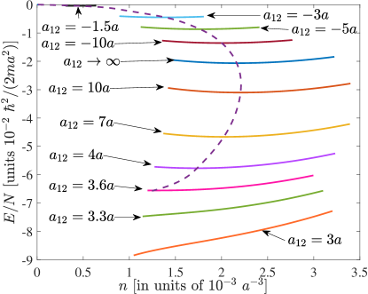
Figure 1: Three-dimensional energy per particle $E/N$ of a strongly interacting Bose droplet predicted by the pairing theory, as a function of the density $n$, with increasing interspecies attraction from $a_{12}=-1.5a$ to $a_{12}=\mp\infty$, and finally to $a_{12}=+3.0a$, as indicated in the figure. The dashed line traces the equilibrium density. It ends at $a_{12}\simeq 3.6a$, where the strongly interacting Bose droplet disappears. The energy per particle $E/N$ is measured in units of $10^{-2}\hbar^{2}/(2ma^{2})$ and the density $n$ is in units of $10^{-3}a^{-3}$.

Let us now consider the strongly interacting regime, where interspecies scattering length $\left|a_{12}\right|$ is significantly larger than the intraspecies scattering length $a$. In Fig. 1, we report the density dependence of the energy per particle $E/N$, when the interspecies attraction increases from $a_{12}=-1.5a$ to $a_{12}=-\infty$, crosses the Feshbach resonance (i.e., $a_{12}$ jumps from $-\infty$ to $+\infty$), and further increases towards the formation of tightly bound molecules ($a_{12}\rightarrow 0^{+}$). Remarkably, with increasing interspecies attraction, the energy per particle decreases steadily from the weakly interacting limit (i.e., $a_{12}<-1.5a$, see the top left of the figure, which has been studied in Ref. (Hu2020a, )) to the strongly interacting regime ($a_{12}\rightarrow\pm\infty$). This is very similar to what happens at the fermionic BEC-BCS crossover (NSR1985, ; Hu2006, ; Diener2008, ), which is realized by tuning the attractive interaction between two unlike fermions across a Feshbach resonance (Regal2004, ; Zwierlein2004, ). Here, we always find a minimum in the energy per particle (see the dashed line), until the interspecies scattering length becomes positive and smaller than a threshold $a_{12,\textrm{crit}}\simeq 3.6a$. The existence of a minimum in the energy per particle, i.e., $\partial(E/N)/\partial n=(\mu-E/N)/n=0$, precisely implies the appearance of a self-bound Bose droplet in a vacuum, which has a zero pressure $P=n\mu-E/\mathcal{V}=0$. Therefore, we observe that a Bose droplet may exist in the strongly interacting regime, where the interspecies scattering length diverges. Importantly, the equilibrium density of the droplet, at which the minimum energy per particle is reached, does not significantly increase as the interspecies scattering length diverges. We find that the equilibrium density attains its largest value near the Feshbach resonance and is about a few times larger than the equilibrium density in the weakly coupling regime (i.e., at $a_{12}=-1.5a$).

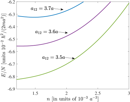
Figure 2: Three-dimensional energy per particle $E/N$ as a function of the density $n$, near the threshold $a_{12}=+3.6a$.

The experimental confirmation of a strongly interacting Bose droplet would be a highly non-trivial task. In a single-component Bose gas, it is well-known that a strongly interacting Bose gas is difficult to reach due to severe three-body loss. Indeed, in the recent experiments the lifetime of a ³⁹K-³⁹K Bose droplet is limited to about ten milliseconds, due to the intraspecies three-body loss in a particular component (i.e., the $\left|F=1,m_{F}=0\right\rangle$ hyperfine state) (Cabrera2018, ; Semeghini2018, ). This is not a serious problem, since we can choose a binary Bose mixture with small intraspecies three-body loss rate, for example, the heteronuclear ⁴¹K-⁸⁷Rb mixture, where the lifetime of the droplet was found to be much longer (DErrico2019, ). As the equilibrium density of a strongly interacting Bose droplet is at the same order as a weakly interacting droplet in magnitude, a large intraspecies three-body loss could be avoided. The fundamental difficulty then may come from the interspecies three-body loss, which remains unknown at the moment. Theoretically, the solution of the three-body problem of two like bosons and one unlike boson and the calculation of the related interspecies three-body loss rate would be an interesting research topic to consider in future works.

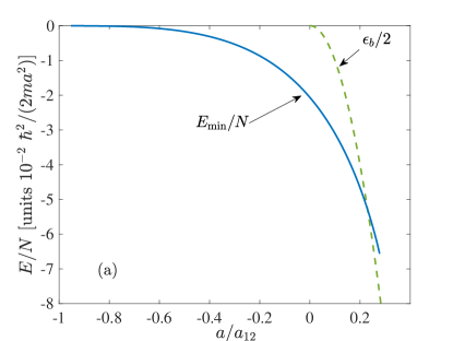
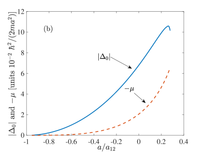
Figure 3: (a) Three-dimensional minimum energy per particle $E_{\min}/N$ as a function of the ratio $a/a_{12}$. The green dashed line shows the half of the bound-state energy $\epsilon_{B}/2$ of a molecule or dimer, formed by two bosons at different species. (b) The pairing order parameter $\Delta_{0}$ (solid line) and the chemical potential $-\mu$ (dashed line), as a function of the ratio $a/a_{12}$. The minimum energy per particle $E_{\min}/N$, the pairing order parameter $\Delta_{0}$, and the chemical potential $-\mu$ are all measured in units of $10^{-2}\hbar^{2}/(2ma^{2})$.

On the BEC side of the Feshbach resonance, the Bose droplet ceases to exist below the threshold $a_{12,\textrm{crit}}\simeq 3.6a$, as highlighted in Fig. 2. This is closely related to the formation of a gas of dimers towards the BEC limit, which also happens at the fermionic BEC-BCS crossover (NSR1985, ; Hu2006, ; Diener2008, ). To show this, in Fig. 3(a) we present the minimum energy per particle $E_{\min}/N$ and the half of the bound-state energy $\epsilon_{B}/2$ of a dimer, as a function of the ratio $a/a_{12}$. It is readily seen that a gas of non-interacting dimers becomes energetically favorable over a Bose droplet once we pass the crossing point of the two energy curves at $a/a_{12}\simeq 0.23$ or $a_{12}\simeq 4.35a$. Interestingly, the pairing order parameter $\Delta_{0}$ appears to have a maximum around the crossing point, as shown in Fig. 3(b).

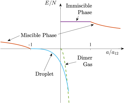
Figure 4: A sketch of the phase diagram of a binary Bose mixture across the bosonic BEC-BCS crossover, illustrated by the energy per particle $E/N$ at a positive and small intraspecies scattering length $0<na^{3}\ll 1$.

The above observation leads us to sketch a general phase diagram for a binary Bose mixture across the Feshbach resonance for the attractive interspecies interactions, as illustrated in Fig. 4. When we increase the interspecies attraction from $a_{12}=0^{-}$ (i.e., the far-left part of the figure), the mixture is initially in the miscible phase. Upon reaching the mean-field collapsing point at $a_{12}=-a$, it turns into a weakly interacting Bose droplet as experimentally observed (Cabrera2018, ; Semeghini2018, ). Across the Feshbach resonance ($a/a_{12}=0$), the Bose droplet becomes strongly interacting with a significant portion of Cooper pairs, whose size is comparable to the mean-distance between bosons. By further increasing the interspecies attraction to the threshold $a_{12,\textrm{crit}}\simeq 3.6a$, the Bose droplet disappears and changes into a gas of dimers via a first-order transition.

It is worth noting that, since the intraspecies scattering length $a$ is small, the interspecies scattering length $a_{12}$ at the threshold would also be small and positive. This means that the gas of dimers would be extremely difficult to reach adiabatically in the time scale of actual experiments, due to its deep energy level. Instead, we would observe a metastable state of the mixture, which is an immiscible phase (i.e., a phase-separation phase where the two components do not overlap in real space) at the threshold $a_{12,\textrm{crit}}\simeq 3.6a$. By further increasing the interspecies attraction towards a vanishing scattering length ($a_{12}\rightarrow 0^{+}$), the mixture will again enter a miscible phase at $a_{12}=a$ and connect smoothly to the miscible phase at $a_{12}=0^{-}$.

V One-dimensional quantum droplets

We now turn to discuss low-dimensional quantum droplets, starting from the one-dimensional case. In one dimension, the contact interaction is well defined and does not need regularization. The interaction strength can be characterized by using the dimensionless interaction parameter, such as $\gamma=mg/(n\hbar^{2})=-2/(na)$ and $\eta=mg_{12}/(n\hbar^{2})=-2/(na_{12})$, where

$$a = -\frac{2\hbar^{2}}{mg}<0$$ (60)

$$a_{12} = -\frac{2\hbar^{2}}{mg_{12}}>0$$ (61)

are the one-dimensional $s$-wave scattering lengths. Following Ref. (Parisi2019, ), we choose the binding energy of a dimer of two bosons in different species, i.e.,

$$\varepsilon_{B}=\frac{\hbar^{2}}{ma_{12}^{2}},$$ (62)

as the units of energy, and the inverse scattering length $\left|a\right|^{-1}$ as the units of density.

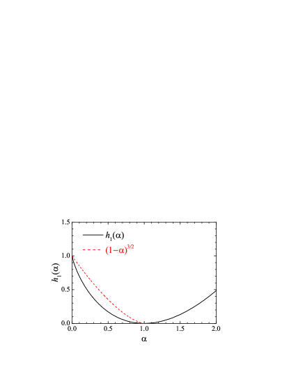
Figure 5: The function $h_{1}(\alpha)$ (solid line) and its comparison to $(1-\alpha)^{3/2}$ (dashed line).

In the Bogoliubov theory, the LHY thermodynamic potential Eq. (41) in one dimension is easy to calculate. By performing the one-dimensional integration,

$$\sum_{\mathbf{k}}\left[\sqrt{\varepsilon_{\mathbf{k}}\left(\varepsilon_{\mathbf{k}}+\alpha\right)}-\varepsilon_{\mathbf{k}}-\frac{\alpha}{2}\right]=-\frac{\left(2m\right)^{1/2}\alpha^{3/2}}{3\pi\hbar},$$ (63)

we obtain

$$\varOmega_{\textrm{LHY}}=-\frac{2m^{1/2}}{3\pi\hbar}\left[\left(C+D\right)^{3/2}+\left(C-D\right)^{3/2}\right].$$ (64)

By taking $C=gn/2$ and $D=g_{12}n/2$ as before in $\varOmega_{\textrm{LHY}}$ and adding the mean-field energy $(g+g_{12})n^{2}/4$, we obtain the energy per particle predicted by the Bogoliubov theory,

$$\frac{E_{\textrm{1D}}}{N}=\left(g+g_{12}\right)\frac{n}{4}-\frac{\left(2m\right)^{1/2}}{6\pi\hbar}g^{3/2}\mathcal{F}_{1}\left(\frac{g_{12}}{g}\right)n^{1/2},$$ (65)

where $\mathcal{F}_{1}(\alpha)\equiv(1+\alpha)^{3/2}+(1-\alpha)^{3/2}$. It is interesting to note that, in one dimension the LHY energy functional is negative so the force provided by quantum fluctuations is attractive. It is to be balanced by the repulsive mean-field force at $g>-g_{12}>0$. Therefore, somehow counterintuitively, the formation of quantum droplets is driven by quantum fluctuations (Petrov2016, ). As the mean-field solution is stable, the energy in Eq. (65) does not suffer from the issue of complex number as we encounter earlier in three dimensions. Nevertheless, following Ref. (Petrov2016, ) we may still use the Petrov’s prescription and take $g_{12}=-g$ in Eq. (65) to define an energy per particle,

$$\frac{E_{\textrm{1D}}}{N}=\left(g+g_{12}\right)\frac{n}{4}-\frac{2m^{1/2}}{3\pi\hbar}g^{3/2}n^{1/2}.$$ (66)

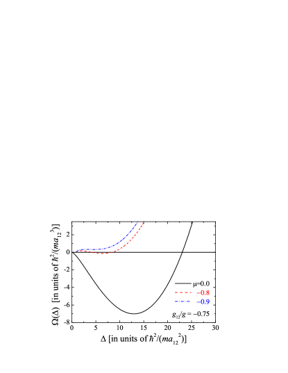
Figure 6: One-dimensional thermodynamic potential $\varOmega_{\textrm{1D}}$, in units of $\hbar^{2}/(ma_{12}^{3})=\varepsilon_{B}a_{12}^{-1}$, as a function of the pairing parameter $\Delta$, at different chemical potentials $\mu=0$ (solid line), $-0.8$ (dashed line), and $-0.9$ (dot-dashed line), and at $g_{12}=-0.75g$. Both $\Delta$ and $\mu$ are measured in units of $\varepsilon_{B}$.

In the pairing theory, we calculate the thermodynamic potential Eq. (30) in one dimension. As in the three-dimensional case, we similarly separate the LHY thermodynamic potential into two parts, $\mathcal{I}_{-}$ and $\mathcal{I}_{+}$. It is straightforward to obtain $\mathcal{I}_{-}$ with the help of the identity Eq. (63) and we obtain,

$$\mathcal{I}_{-}=-\frac{4m^{1/2}}{3\pi\hbar}C^{3/2}\left(1+\frac{\Delta}{C}\right)^{3/2}.$$ (67)

For $\mathcal{I}_{+}$, we instead find

$$\mathcal{I}_{+}=-\frac{4m^{1/2}}{3\pi\hbar}C^{3/2}h_{1}\left(\alpha\right),$$ (68)

where the function $h_{1}(\alpha)$ is given by,

$$h_{1}\equiv 3\int_{0}^{\infty}dt\left[t^{2}+\frac{1+\alpha}{2}-\sqrt{\left(t^{2}+1\right)\left(t^{2}+\alpha\right)}\right],$$ (69)

and is plotted in Fig. 5. Therefore, we obtain the total thermodynamic potential ($C=\mu+\Delta$),

$$\varOmega_{\textrm{1D}}=-\frac{C^{2}}{g}-\frac{\Delta^{2}}{g_{12}}-\frac{2m^{1/2}}{3\pi\hbar}C^{3/2}\mathcal{G}_{1}\left(\frac{\Delta}{C}\right),$$ (70)

where $\mathcal{G}_{1}(\alpha)\equiv(1+\alpha)^{3/2}+h_{1}(\alpha)$.

In Fig. 6, we show the thermodynamic potential $\varOmega_{\textrm{1D}}$ as a function of $\Delta$ at the interspecies interaction strength $g_{12}=-0.75g$. The curves at three different chemical potentials $\mu=0$, $-0.8$, and $-0.9$, measured in units of $\varepsilon_{B}$, are plotted. When the chemical potential is above a critical value, i.e., $\mu_{c}\simeq-0.8\varepsilon_{B}$, we typically find a global minimum in the thermodynamic potential at $\Delta_{0}\neq 0$. For $\mu<\mu_{c}$, the global minimum turns into a local minimum and hence the saddle-point pairing parameter takes the trivial solution $\Delta_{0}=0$. As a result, there is a jump in $\Delta_{0}$ when we tune the chemical potential across $\mu_{c}$. Physically, this indicates a first-order quantum phase transition from a droplet phase to a gas-like expanding phase. In other words, when the density $n$ is very dilute (at $\mu<\mu_{c}$), the attractive force provided by quantum fluctuations (i.e., the LHY energy $\propto n^{3/2}$) is unstable to balance the repulsive mean-field force (i.e., characterized by the mean-field energy $\propto n^{2}$). Thus, the expansion of the gas-like phase can no longer be prevented.

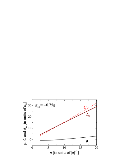
Figure 7: One-dimensional chemical potential $\mu$, the parameter $C$ and the pairing gap $\Delta_{0}$, in units of $\varepsilon_{B}$, as a function of the total density $n$ (in units of $\left|a\right|^{-1}$) at $g_{12}=-0.75g$.

By finding the saddle-point solution $\Delta=\Delta_{0}\neq 0$ through the minimization of $\varOmega(\Delta)$, we consequently calculate the density $n=-\partial\varOmega(\mu,\Delta_{0})/\partial\mu$. The resulting parameter $C=\mu+\Delta_{0}$ and the pairing gap $\Delta_{0}$, together with the chemical potential $\mu$, are shown in Fig. 7 as a function of the density $n$, at a typical interspecies interaction strength $g_{12}=-0.75g$. Here, we are always in the weak-coupling regime, since the dimensionless interaction parameters such as $\gamma=2/(n\left|a\right|)<1$. Unlike the three-dimensional case, the condition $\left|\mu\right|\ll C,\Delta_{0}$ seems to be less satisfied at low densities, where we see a clear difference between $C$ and $\Delta_{0}$. Therefore, although an approximate analytical energy equation can still be derived, i.e.,

$$\frac{E_{\textrm{1D}}}{N}=-\left(g+\frac{g^{2}}{g_{12}}\right)\frac{n}{4}-\frac{2m^{1/2}}{3\pi\hbar}g^{3/2}n^{1/2},$$ (71)

we would prefer to use the full numerical calculation. A comparison between the numerical and analytical results of our pairing theory at the interspecies interaction strength $g_{12}=-0.75g$ is shown in Appendix A.

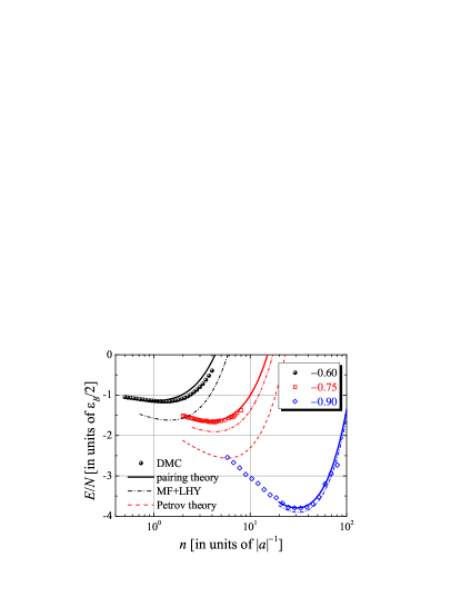
Figure 8: One-dimensional energy per particle as a function of the density at three interspecies interaction strengths $g_{12}/g=-0.60$ (black), $-0.75$ (red) and $-0.90$ (blue). Our pairing results (solid lines) are compared with the recent DMC data (symbols) (Parisi2019, ), the MF+LHY predictions Eq. (65) (dot-dashed lines), and the MF+LHY results with Petrov’s prescription Eq. (66) (dashed line, for $g_{12}/g=-0.75$ only). The energy is in units of $\varepsilon_{B}/2$ and the density is in units of $\left|a\right|^{-1}$.

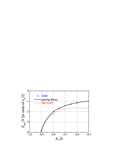
Figure 9: Minimum energy per particle $E_{\min}/N$ or equilibrium chemical potential $\mu_{\textrm{eq}}$ in one dimension as a function of the interspecies interaction strength $g_{12}/g$, obtained from the pairing theory (solid line), the DMC simulation (circles) (Parisi2019, ) and the MF+LHY theory Eq. (65) (dot-dashed line). The energy is in units of $\varepsilon_{B}/2$.

In Fig. 8, we present the energy per particle predicted by the pairing theory at three interspecies interactions $g_{12}/g=-0.60$ (black), $-0.75$ (red) and $-0.90$ (blue) by solid lines, and compare them to the available DMC data taken from Ref. (Parisi2019, ) (symbols), to the Bogoliubov results Eq. (65) (dot-dashed lines), and to the Bogoliubov prediction with Petrov’s prescription Eq. (66) (dashed line) (Petrov2016, ). We find an excellent agreement between our pairing theory and the state-of-the-art DMC simulation at all three interaction strengths. The agreement at $g_{12}=-0.60g$ is particularly impressive, as the dimensionless density $n\left|a\right|$ decreases and becomes close to unity so the dimensionless interaction parameter $\gamma=2/(n\left|a\right|)\sim O(1)$ is large. We would rather anticipate the breakdown of the Bogoliubov approximation, which our pairing theory relies on. Indeed, at this interaction strength the conventional Bogoliubov prediction Eq. (65) already shows significant deviation from the DMC data. We attribute the good agreement between our theory and the DMC simulation to our reasonable description of the bosonic pairing.

To understand this, it is useful show the chemical potential $\mu_{\textrm{eq}}$ at the equilibrium density (or the minimum energy per particle $E_{\min}/N$) as a function of the interspecies interaction strength $g_{12}/g$, as reported in Fig. 9. The excellent agreement between our pairing theory and the DMC simulation for the equilibrium chemical potential $\mu_{\textrm{eq}}$ is fairly evident, up to a critical interspecies interaction strength $(g_{12}/g)_{\textrm{crit}}\sim-0.47(2)$ as predicted by the DMC (Parisi2019, ). Towards the critical interaction strength, the equilibrium chemical potential quickly approaches the half of the binding energy of a dimer, i.e., $-\varepsilon_{B}/2$, indicating that the system could be understood as a collection of weakly-interacting dimers. This interpretation is reasonable, as the DMC threshold $(g_{12}/g)_{\textrm{crit}}\sim-0.47(2)$ is close to the zero-crossing in the effective dimer-dimer interaction $(g_{12}/g)_{0}\sim-0.45$ (Pricoupenko2018, ).

Our pairing theory precisely provides a useful description of those weakly-interacting dimers at the mean-field level, since we take a uniform pairing gap in the saddle point solution. Thus, we anticipate the pairing theory may predict a similar critical interspecies interaction strength as in the DMC simulation. By determining the equilibrium density $n_{\textrm{eq}}$ at different interspecies interactions near the zero-crossing of dimer-dimer scattering, we find the equilibrium density vanishes at $(g_{12}/g)_{\textrm{crit}}\sim-0.35$, which seems to be consistent with the DMC prediction (Parisi2019, ) and the few-body zero-crossing result (Pricoupenko2018, ).

VI Two-dimensional quantum droplets

We finally consider two-dimensional quantum droplets. In two dimensions, the regularization of the bare interaction strength becomes subtle due to the logarithmic infrared divergence at low energy, which we may remove by introducing an arbitrary energy scale $\varepsilon_{c}$, i.e.,

$$\frac{1}{g} = \frac{m}{4\pi\hbar^{2}}\ln\left(\frac{4\hbar^{2}}{e^{2\gamma}ma^{2}\varepsilon_{c}}\right)-\sum_{\mathbf{k}}\frac{1}{2\varepsilon_{\mathbf{k}}+\varepsilon_{c}},$$ (72)

$$\frac{1}{g_{12}} = \frac{m}{4\pi\hbar^{2}}\ln\left(\frac{4\hbar^{2}}{e^{2\gamma}ma_{12}^{2}\varepsilon_{c}}\right)-\sum_{\mathbf{k}}\frac{1}{2\varepsilon_{\mathbf{k}}+\varepsilon_{c}}.$$ (73)

Here, $\gamma\simeq 0.577216$ is Euler–Mascheroni constant, $a$ and $a_{12}$ are two-dimensional $s$-wave scattering lengths. Alternatively, we may consider the use of the binding energies $E_{T}\equiv 4\hbar^{2}/(e^{2\gamma}ma^{2})$ and $E_{S}\equiv 4\hbar^{2}/(e^{2\gamma}ma_{12}^{2})$, where analogous to the fermionic case the subscripts “$T$” and “$S$” emphasize the tendency of the formation of triplet and singlet pairs for bosons in the same-species and unlike-species, respectively. We then rewrite the bare interaction strengths in a simpler form,

$$\frac{1}{g} = -\sum_{\mathbf{k}}\frac{1}{\hbar^{2}\mathbf{k}^{2}/m+E_{T}},$$ (74)

$$\frac{1}{g_{12}} = -\sum_{\mathbf{k}}\frac{1}{\hbar^{2}\mathbf{k}^{2}/m+E_{S}}.$$ (75)

In this section, we use $E_{T}$ and $a^{-2}$ as the units of energy and density, respectively.

In the Bogoliubov theory, the approximate energy of quantum droplets was derived by Petrov and Astrakharchik in Ref. (Petrov2016, ). For $\ln(a_{12}/a)\gg 1$, it takes the form (Petrov2016, ),

$$\frac{E_{\textrm{2D}}}{N}=\frac{2\pi n}{\ln^{2}\left(a_{12}/a\right)}\left[\ln\left(\frac{n}{n_{\textrm{eq}}}\right)-1\right],$$ (76)

where the equilibrium density is

$$n_{\textrm{eq}}a^{2}=\frac{e^{-2\gamma-3/2}}{\pi}\frac{\ln\left(a_{12}/a\right)}{\left(a_{12}/a\right)}.$$ (77)

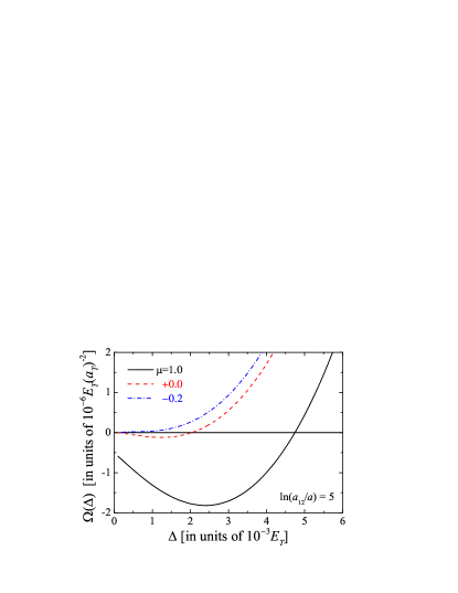
Figure 10: Two-dimensional thermodynamic potential $\varOmega_{\textrm{2D}}$, in units of $10^{-6}E_{T}a_{T}^{-2}$, as a function of the pairing parameter $\Delta$, at different chemical potentials $\mu=1.0$ (solid line), $0$ (dashed line), and $-0.2$ (dot-dashed line), and at the interspecies interaction strength $\ln(a_{12}/a)=5$. Both $\Delta$ and $\mu$ are measured in units of $10^{-3}E_{T}$.

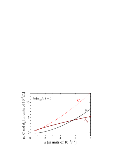
Figure 11: Two-dimensional chemical potential $\mu$, the parameter $C$ and the pairing gap $\Delta_{0}$, in units of $10^{-3}E_{T}$, as a function of the total density $n$ (in units of $10^{-3}a^{-2}$) at $\ln(a_{12}/a)=5$.

In our pairing theory, by replacing the bare interaction strengths with the binding energies, the thermodynamic potential can be written as ($C=\mu+\Delta$),

$$\varOmega_{\textrm{2D}} = \frac{1}{2}\sum_{\mathbf{k}}\left[E_{+}\left(\mathbf{k}\right)+E_{-}\left(\mathbf{k}\right)-2\left(\varepsilon_{\mathbf{k}}+C+\Delta\right)\right.$$ (78)

$$\left.+\frac{2C^{2}}{2\varepsilon_{\mathbf{k}}+E_{T}}+\frac{2\Delta^{2}}{2\varepsilon_{\mathbf{k}}+E_{S}}\right].$$

It is interesting to see that the condensate term now disappears after regularization. This also happens if we choose the regularization through Eq. (72) and Eq. (73), since the cut-off energy $\varepsilon_{c}$ can be arbitrarily selected. The same trick was used in Ref. (Petrov2016, ) to derive the Bogoliubov result Eq. (76). A vanishing condensate term is related to the fact that in two dimensions, the small interaction parameter is given by $1/\ln(na^{2})$ and one has to include the LHY term in the energy, in order to have a meaningful perturbative expansion expression for the energy (Schick1971, ). As the controlling parameter is only logarithmically small, as we shall see, it appears more challenging to obtain an accurate result within perturbation theories.

The integration in Eq. (78) can be performed analytically, as in usual two-dimensional mean-field theories. We find that,

$$\varOmega_{\textrm{2D}} = \frac{m}{4\pi\hbar^{2}}\left[C\Delta-C_{2}\sqrt{C\Delta}+\frac{\mu^{2}}{4}\ln\left(\sqrt{C}+\sqrt{\Delta}\right)\right.$$ (79)

$$\left.+\frac{C_{2}^{2}}{2}\ln\left(eC_{2}\right)-C^{2}\ln E_{T}-\Delta^{2}\ln E_{S}\right],$$

where $C_{2}\equiv C+\Delta=\mu+2\Delta$. In Fig. 10, we examine the $\Delta$-dependence of the thermodynamic potential at the interspecies interaction strength $\ln(a_{12}/a)=5$. It clearly shows a global minimum when the chemical potential is above a threshold, similar to the three-dimensional and one-dimensional cases. Therefore, we determine the saddle-point pairing gap $\Delta_{0}$ and consequently calculate the density and total energy. The resulting parameter $C$ and the pairing gap $\Delta_{0}$ are shown in Fig. 11, as a function of the density $n$. The chemical potential $\mu$ is also shown. We find that with increasing the density, the chemical potential $\mu$ increases rapidly and is larger than the pairing gap $\Delta_{0}$ at sufficiently large densities.

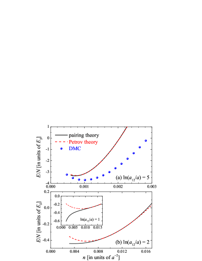
Figure 12: Two-dimensional energy per particle as a function of the density at three interspecies interaction strengths $\ln(a_{12}/a)=5$ (a), $\ln(a_{12}/a)=2$ (b), and $\ln(a_{12}/a)=1$ (inset in (b)). Our pairing results (solid lines) are compared with the MF+LHY predictions with Petrov’s theory Eq. (76) (dashed line). In (a), we show also the DMC data from Ref. (Petrov2016, ). The energy is in units of the interspecies binding energy $E_{S}$ and the density is in units of $a^{-2}$. We note that the scales of energy and density change by a factor of $\sim 10$ in the upper and lower panels.

In Fig. 12, we report the density dependence of the energy per particle of two-dimensional quantum droplets at two interspecies interaction strengths, $\ln(a_{12}/a)=5$ (a) and $\ln(a_{12}/a)=2$ (b). Our pairing results are compared with Petrov’s prediction Eq. (76) and the DMC data (for $\ln(a_{12}/a)=5$ only) (Petrov2016, ). For a weak interspecies interaction, as shown in Fig. 12(a), there is a very close agreement between our pairing result and Petrov’s result. Both of them seems to strongly over-estimate the energy, in comparison to the benchmark DMC data, in spite of the weak interspecies interaction. This is understandable: as we mentioned earlier, it is difficult to have accurate perturbative expansion in two dimensions due to the logarithmically small controlling parameter. To improve the accuracy of theoretical prediction, we need to go beyond the Bogoliubov approximation and to obtain the correction beyond LHY following, for example, the procedure by Mora and Castin in Ref. (Mora2009, ) for a scalar two-dimensional weakly-interacting Bose gas. This will be considered in our future works.

At a larger interspecies interaction, as illustrated in Fig. 12(b), the difference between the pairing result and Petrov’s result becomes noticeable. In particular, at small densities the pairing theory predicts a lower energy. In this regime, we anticipate that the pairing effect start to become significant, so the explicit inclusion of the bosonic pairing, just as we consider in the pairing theory, improve the energy.

Remarkably, by further increasing the interspecies interaction, as can be seen from the inset of Fig. 12(b), we find that the energy per particle predicted by the pairing theory decreases monotonically with decreasing density. There is no minimum in the energy per particle, to support a self-bound liquid-like droplet with zero pressure in vacuum. This is not a surprising result, as we already find the similar situation in one dimension, where the one-dimensional quantum droplet can disappear and turn into a bright soliton, when the interspecies attraction stronger than the threshold $(g_{12})_{\textrm{crit}}=-g$ (Tylutki2020, ). By plotting the energy curve at different interspecies interactions, we determine a threshold in two dimensions, $[\ln(a_{12}/a)]_{\textrm{crit}}\sim 1.9$, below which the droplet changes its fundamental characters and presumably turns into a soliton-like many-particle bound state (Hammer2004, ; Bazak2018, ). Incidentally, this threshold is close to the zero-crossing of the effective dimer-dimer interaction in two dimensions, i.e., $[\ln(a_{12}/a)]_{\textrm{0}}\simeq\ln(10)\simeq 2.3$, obtained from the few-body calculations (Guijarro2020, ).

Dimensions	Formation threshold	Disappearance threshold
One	$\left(a_{12}/a\right)^{-1}\simeq-0.35$	$a_{12}/a=-1$
Two	$\ln^{-1}\left(a_{12}/a\right)=0$	$\ln^{-1}\left(a_{12}/a\right)\simeq 0.52$
Three	$a_{12}=-a$	$a_{12}\simeq 3.6a$

Table 1: Thresholds for quantum droplet formation and disappearance in one, two and three dimensions in terms of the $s$-wave scattering lengths, predicted by the pairing theory.

VII Conclusions

In summary, we have presented a systematic investigation of bulk properties of utradilute quantum droplets in a Bose-Bose mixture, by using the recently developed pairing theory (Hu2020a, ). We have focused on the low-dimensional droplets, and have found that the bosonic pairing plays an increasingly important role in low dimensions, particularly near the threshold at which the self-bound droplets start to emerge or disappear, as listed in Table 1. We have also considered a strongly interacting quantum droplet in three dimensions.

In one dimension, we have shown that the energy per particle predicted by our pairing theory agrees excellent well with the numerically accurate diffusion Monte Carlo data (Parisi2019, ), at all the interaction strengths where the simulation data are available (which also nearly cover the phase window where one-dimensional quantum droplets exist). Our pairing theory also predicts a critical interspecies attraction for the emergence of droplets, i.e., $(g_{12}/g)_{\textrm{crit}}\sim-0.35$, which is consistent with the DMC prediction $(g_{12}/g)_{\textrm{crit}}\sim-0.47(2)$ (Parisi2019, ) and with the zero-crossing point $(g_{12}/g)_{0}\sim-0.45$ where the effective dimer-dimer interaction changes from repulsive to attractive (Pricoupenko2018, ).

In two dimensions, quantum droplets form for an arbitrary small interspecies attraction. We have found our pairing theory becomes less efficient, due to the weak interspecies attraction for pairing and the logarithmically small controlling parameters that disfavors the development of accurate perturbation theories. Yet, our pairing theory still provides an improvement compared with the prototype theory of two-dimensional quantum droplets developed earlier (Petrov2016, ). With increasing interspecies attractions, the pairing theory seems to become more useful. We have predicted a threshold $[\ln(a_{12}/a)]_{\textrm{crit}}\sim 1.9$, below which the droplet may turn into a many-particle bound state predicted earlier by Hammer and Son (Hammer2004, ). Interestingly, such a threshold is close to the zero-crossing $[\ln(a_{12}/a)]_{\textrm{0}}\simeq 2.3$ of the effective dimer-dimer interaction in two dimensions found through few-body calculations (Guijarro2020, ).

In three dimensions, we have shown an exciting possibility of realizing the so-called bosonic BEC-BCS crossover, by tuning the interspecies scattering length $a_{12}$ to be infinitely large near a Feshbach resonance. The superfluid properties of the resulting strongly interacting quantum droplet are to be explored. We anticipate that it may have some universal behaviors in collective dynamics and thermodynamics, analogous to its fermionic counterpart. Across the Feshbach resonance, we have found that the strongly interacting quantum droplet disappears at about $a_{12}\simeq 3.6a$.

In future studies, it would be interesting to use our microscopic pairing theory to directly investigate the profile and the collective excitations of quantum droplets, without the use of the local density approximation or density functional theories. These fundamental properties are important for characterizing ultradilute quantum droplets in ultracold atomic laboratories.

Appendix A Analytic energy expression in one dimension

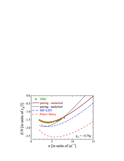
Figure 13: One-dimensional energy per particle as a function of the density at the interspecies interaction strength $g_{12}=-0.75g$. Our pairing results (numerical - brown thick solid line, and analytical - black thin solid line, see Eq. (71)) are compared with the recent DMC data (symbols with error bars) (Parisi2019, ), the MF+LHY prediction Eq. (65) (dot-dashed lines), and the MF+LHY results with Petrov’s prescription Eq. (66) (dashed line). The energy is in units of $\varepsilon_{B}/2$ and the density is in units of $\left|a\right|^{-1}$.

In Fig. 13, we show the numerical and analytical results of our pairing theory for the one-dimensional energy per particle at the interspecies interaction strength $g_{12}=-0.75g$. The analytical expression Eq. (71) does not provide a good approximation to the numerical result, since unlike in the three-dimensional case the assumption $\left|\mu\right|\ll C,\Delta_{0}$ is not satisfied so well.

References

- (1) F. Dalfovo, S. Giorgini, L. P. Pitaevskii, and S. Stringari, Theory of Bose-Einstein condensation in trapped gases, Rev. Mod. Phys. 71, 463 (1999).
- (2) E. A. Donley, N. R. Claussen, S. L. Cornish, J. L. Roberts, E. A. Cornell, and C. E. Wieman, Dynamics of collapsing and exploding Bose–Einstein condensates, Nature (London) 412, 295 (2001).
- (3) D. S. Petrov, Quantum Mechanical Stabilization of a Collapsing Bose-Bose Mixture, Phys. Rev. Lett. 115, 155302 (2015).
- (4) T. D. Lee, K. Huang, and C. N. Yang, Eigenvalues and Eigenfunctions of a Bose System of Hard Spheres and Its Low-Temperature Properties, Phys. Rev. 106, 1135 (1957).
- (5) D. S. Petrov, Liquid beyond the van der Waals paradigm, Nat. Phys. 14, 211 (2018).
- (6) I. Ferrier-Barbut, Ultradilute Quantum Droplets, Phys. Today 72, 46 (2019).
- (7) Y. Kartashov, G. Astrakharchik, B. Malomed, and L. Torner, Frontiers in multidimensional self-trapping of nonlinear fields and matter, Nat. Rev. Phys. 1, 185 (2019).
- (8) I. Ferrier-Barbut, H. Kadau, M. Schmitt, M. Wenzel, and T. Pfau, Observation of Quantum Droplets in a Strongly Dipolar Bose Gas, Phys. Rev. Lett. 116, 215301 (2016).
- (9) M. Schmitt, M. Wenzel, F. Böttcher, I. Ferrier-Barbut, and T. Pfau, Self-bound droplets of a dilute magnetic quantum liquid, Nature (London) 539, 259 (2016).
- (10) L. Chomaz, S. Baier, D. Petter, M. J. Mark, F. Wächtler, L. Santos, and F. Ferlaino, Quantum-Fluctuation-Driven Crossover from a Dilute Bose-Einstein Condensate to a Macrodroplet in a Dipolar Quantum Fluid, Phys. Rev. X 6, 041039 (2016).
- (11) F. Böttcher, M. Wenzel, J.-N. Schmidt, M. Guo, T. Langen, I. Ferrier-Barbut, T. Pfau, R. Bombín, J. Sánchez-Baena, J. Boronat, and F. Mazzanti, Dilute dipolar quantum droplets beyond the extended Gross-Pitaevskii equation, Phys. Rev. Research 1, 033088 (2019).
- (12) F. Böttcher, J.-N. Schmidt, M. Wenzel, J. Hertkorn, M. Guo, T. Langen and T. Pfau, Transient Supersolid Properties in an Array of Dipolar Quantum Droplets, Phys. Rev. X 9, 011051 (2019).
- (13) C. Cabrera, L. Tanzi, J. Sanz, B. Naylor, P. Thomas, P. Cheiney, and L. Tarruell, Quantum liquid droplets in a mixture of Bose-Einstein condensates, Science 359, 301 (2018).
- (14) P. Cheiney, C. R. Cabrera, J. Sanz, B. Naylor, L. Tanzi, and L. Tarruell, Bright Soliton to Quantum Droplet Transition in a Mixture of Bose-Einstein Condensates, Phys. Rev. Lett. 120, 135301 (2018).
- (15) G. Semeghini, G. Ferioli, L. Masi, C. Mazzinghi, L. Wolswijk, F. Minardi, M. Modugno, G. Modugno, M. Inguscio, and M. Fattori, Self-Bound Quantum Droplets of Atomic Mixtures in Free Space, Phys. Rev. Lett. 120, 235301 (2018).
- (16) G. Ferioli, G. Semeghini, L. Masi, G. Giusti, G. Modugno, M. Inguscio, A. Gallemi, A. Recati, and M. Fattori, Collisions of Self-Bound Quantum Droplets, Phys. Rev. Lett. 122, 090401 (2019).
- (17) C. D’Errico, A. Burchianti, M. Prevedelli, L. Salasnich, F. Ancilotto, M. Modugno, F. Minardi, and C. Fort, Observation of quantum droplets in a heteronuclear bosonic mixture, Phys. Rev. Research 1, 033155 (2019).
- (18) For a recent review, see, for example, F. Böttcher, J.-N. Schmidt, J. Hertkorn, K. S. H. Ng, S. D. Graham, M. Guo, T. Langen, and T. Pfau, New states of matter with fine-tuned interactions: quantum droplets and dipolar supersolids, arXiv:2007.06391 (2020).
- (19) D. S. Petrov and G. E. Astrakharchik, Ultradilute Low-Dimensional Liquids, Phys. Rev. Lett. 117, 100401 (2016).
- (20) D. Baillie, R. M. Wilson, R. N. Bisset, and P. B. Blakie, Self-bound dipolar droplet: A localized matter wave in free space, Phys. Rev. A 94, 021602(R) (2016).
- (21) F. Wächtler and L. Santos, Ground-state properties and elementary excitations of quantum droplets in dipolar Bose-Einstein condensates, Phys. Rev. A 94, 043618 (2016).
- (22) D. Baillie, R. M. Wilson, and P. B. Blakie, Collective Excitations of Self-Bound Droplets of a Dipolar Quantum Fluid, Phys. Rev. Lett. 119, 255302 (2017).
- (23) Y. Li, Z. Luo, Y. Liu, Z. Chen, C. Huang, S. Fu, H. Tan, and B. A. Malomed, Two-dimensional solitons and quantum droplets supported by competing self- and cross-interactions in spin-orbit-coupled condensates, New J. Phys. 19, 113043 (2017).
- (24) A. Cappellaro, T. Macrì, G. F. Bertacco, and L. Salasnich, Equation of state and self-bound droplet in Rabi-coupled Bose mixtures, Sci. Rep. 7, 13358 (2017).
- (25) N. B. Jørgensen, G. M. Bruun, and J. J. Arlt, Dilute Fluid Governed by Quantum Fluctuations, Phys. Rev. Lett. 121, 173403 (2018).
- (26) X. Cui, Spin-orbit-coupling-induced quantum droplet in ultracold Bose-Fermi mixtures, Phys. Rev. A 98, 023630 (2018).
- (27) C. Staudinger, F. Mazzanti and R. E. Zillich, Self-bound Bose mixtures, Phys. Rev. A 98, 023633 (2018).
- (28) L. Parisi, G. E. Astrakharchik, and S. Giorgini, Liquid State of One-Dimensional Bose Mixtures: A Quantum Monte Carlo Study, Phys. Rev. Lett. 122, 105302 (2019).
- (29) V. Cikojević, L. Vranješ Markic, G. E. Astrakharchik, and J. Boronat, Universality in ultradilute liquid Bose-Bose mixtures, Phys. Rev. A 99, 023618 (2019).
- (30) M. Tylutki, G. E. Astrakharchik, B. A. Malomed, and D. S. Petrov, Collective excitations of a one-dimensional quantum droplet, Phys. Rev. A 101, 051601(R) (2020).
- (31) T. Shi, J. Pan, and S. Yi, Trapped Bose-Einstein Condensates with Attractive -wave Interaction, arXiv:1909.02432 (2019).
- (32) V. Cikojević, L. Vranješ Markić, and J. Boronat, Finite-range effects in ultradilute quantum drops, arXiv:2001.09086 (2020).
- (33) Y. Wang, L. Guo, S. Yi, and T. Shi, Theory for Self-Bound States of Dipolar Bose-Einstein Condensates, arXiv:2002.11298 (2020).
- (34) H. Hu and X.-J. Liu, Consistent theory of self-bound quantum droplets with bosonic pairing, arXiv:2005.08581 (2020).
- (35) M. Ota and G. E. Astrakharchik, Beyond Lee-Huang-Yang description of self-bound Bose mixtures, arXiv:2005.10047 (2020).
- (36) D. M. Larsen, Binary mixtures of dilute Bose gases with repulsive interactions at low temperature, Ann. Phys. (N.Y.) 24, 89 (1963).
- (37) J. Bardeen, L. N. Cooper, and J. R. Schrieffer, Microscopic Theory of Superconductivity, Phys. Rev. 106, 162 (1957).
- (38) P. Nozières and S. Schmitt-Rink, Bose condensation in an attractive fermion gas: From weak to strong coupling superconductivity, J. Low Temp. Phys. 59, 95 (1985).
- (39) H. Hu, X.-J. Liu, and P. D. Drummond, Equation of state of a superfluid Fermi gas in the BCS-BEC crossover, Europhys. Lett. 74, 574 (2006).
- (40) R. B. Diener, R. Sensarma, and M. Randeria, Quantum fluctuations in the superfluid state of the BCS-BEC crossover, Phys. Rev. A 77, 023626 (2008).
- (41) C. A. Regal, M. Greiner, and D. S. Jin, Observation of Resonance Condensation of Fermionic Atom Pairs, Phys. Rev. Lett. 92, 040403 (2004).
- (42) M. W. Zwierlein, C. A. Stan, C. H. Schunck, S. M. F. Raupach, A. J. Kerman, and W. Ketterle, Condensation of Pairs of Fermionic Atoms near a Feshbach Resonance, Phys. Rev. Lett. 92, 120403 (2004).
- (43) C. Mora and Y. Castin, Ground State Energy of the Two-Dimensional Weakly Interacting Bose Gas: First Correction Beyond Bogoliubov Theory, Phys. Rev. Lett. 102, 180404 (2009).
- (44) G. E. Astrakharchik, J. Boronat, J. Casulleras, I. L. Kurbakov, and Yu. E. Lozovik, Equation of state of a weakly interacting two-dimensional Bose gas studied at zero temperature by means of quantum Monte Carlo methods, Phys. Rev. A 79, 051602(R) (2009).
- (45) G. Guijarro, G. E. Astrakharchik, J. Boronat, B. Bazak, and D. S. Petrov, Few-body bound states of two-dimensional bosons, Phys. Rev. A 101, 041602(R) (2020).
- (46) L. He, H. Lü, G. Cao, H. Hu, and X.-J. Liu, Quantum fluctuations in the BCS-BEC crossover of two-dimensional Fermi gases, Phys. Rev. A 92, 023620 (2015).
- (47) H. Hu and X.-J. Liu, Quantum fluctuations in a strongly interacting Bardeen-Cooper-Schrieffer polariton condensate at thermal equilibrium, Phys. Rev. A 101, 011602(R) (2020).
- (48) L. Salasnich and F. Toigo, Zero-point energy of ultracold atoms, Phys. Rep. 640, 1 (2016).
- (49) H. Hu, H. Deng, and X.-J. Liu, Two-dimensional exciton-polariton interactions beyond the Born approximation, arXiv:2004.05559.
- (50) C. Chin, M. Bartenstein, A. Altmeyer, S. Riedl, S. Jochim, J. Hecker Denschlag, and R. Grimm, Observation of the Pairing Gap in a Strongly Interacting Fermi Gas, Science 305, 1128 (2004).
- (51) J. Stenger, S. Inouye, A. P. Chikkatur, D. M. Stamper-Kurn, D. E. Pritchard, and W. Ketterle, Bragg Spectroscopy of a Bose-Einstein Condensate, Phys. Rev. Lett. 82, 4569 (1999).
- (52) A. Pricoupenko and D. S. Petrov, Dimer-dimer zero crossing and dilute dimerized liquid in a one-dimensional mixture, Phys. Rev. A 97, 063616 (2018).
- (53) M. Schick, Two-Dimensional System of Hard-Core Bosons, Phys. Rev. A 3, 1067 (1971).
- (54) H.-W. Hammer and D. T. Son, Universal Properties of Two-Dimensional Boson Droplets, Phys. Rev. Lett. 93, 250408 (2004).
- (55) B. Bazak and D. S. Petrov, Energy of two-dimensional bosons with zero-range interactions, New J. Phys. 20, 023045 (2018).