A Systematic Study on the Absorption Features of Interstellar Ices in Presence of Impurities

Abstract

Spectroscopic studies play a key role in the identification and analysis of interstellar ices and their structure. Some molecules have been identified within the interstellar ices either as pure, mixed, or even as layered structures. Absorption band features of water ice can significantly change with the presence of different types of impurities (CO, $\rm{CO_{2}}$, $\rm{CH_{3}OH}$, $\rm{H_{2}CO}$, etc.). In this work, we carried out a theoretical investigation to understand the behavior of water band frequency, and strength in the presence of impurities. The computational study has been supported and complemented by some infrared spectroscopy experiments aimed at verifying the effect of HCOOH, $\rm{NH_{3}}$, and $\rm{CH_{3}OH}$ on the band profiles of pure $\rm{H_{2}O}$ ice. Specifically, we explored the effect on the band strength of libration, bending, bulk stretching, and free-OH stretching modes. Computed band strength profiles have been compared with our new and existing experimental results, thus pointing out that vibrational modes of $\rm{H_{2}O}$ and their intensities can change considerably in the presence of impurities at different concentrations. In most cases, the bulk stretching mode is the most affected vibration, while the bending is the least affected mode. HCOOH was found to have a strong influence on the libration, bending, and bulk stretching band profiles. In the case of NH₃, the free-OH stretching band disappears when the impurity concentration becomes 50%. This work will ultimately aid a correct interpretation of future detailed spaceborne observations of interstellar ices by means of the upcoming JWST mission.

Department of Physical Sciences, The Open University, Milton Keynes, UK Department of Chemistry, Graduate School of Science and Engineering, Tokyo Metropolitan University, 1-1 Minami-Osawa, Hachioji, Tokyo 192-0397, Japan Astronomical Institute, Tohoku University, Aramakiazaaoba 6-3, Aoba-ku, Sendai, Miyagi, 980-8578, Japan Department of Physical Sciences, The Open University, Milton Keynes, UK

Keywords: Astrochemistry, spectra, ISM: molecules, methods: numerical, experimental, infrared: Band strength, interstellar ice.

1 Introduction

Interstellar grains mainly consist of nonvolatile silicate or carbonaceous compounds covered by icy mantle layers. Interstellar ices play a crucial role in the chemical enrichment of the interstellar medium (ISM). While the existence of interstellar ice was first proposed by Eddington ¹ in 1937, a turning point was marked, more than 40 years later, when Tielens and Hagen ² introduced a combined gas-grain chemistry for the chemical evolution of the ISM. More recently, it has been demonstrated that even pre-biotic molecules can be produced in UV-irradiated astrophysical relevant ices ³. For instance, Nuevo et al. ⁴ experimentally showed that nucleobases can be formed by UV irradiation of pyrimidine in H₂O-rich ice mixtures containing NH₃, CH₃OH, and CH₄.

The composition of interstellar ices can be determined through their absorption spectra in the infrared (IR) region. Since the composition of ISM grain mantles strongly depends on physical conditions ^{5, 6, 7, 8}, the observed spectra can be very different in different astrophysical regions. $\rm{H_{2}O}$ is the most dominant ice component in dense molecular clouds ⁹, accounting for $60-70\%$ of the icy mantels ¹⁰. Water ice was firstly detected through the comparison of ground-based observations of its O-H stretching band at $3278.69$ cm^-1 ($3.05$ $\mu$m) toward Orion-KL ¹¹ and laboratory work by Irvine and Pollack ¹². Since then, several ground-based observations were carried out to identify the signatures of water ice in different astrophysical environments, with further laboratory studies supporting such observations ^{13, 14, 15}. More recently, water was detected by the space-borne Infrared Space Observatory (ISO) mission through its Short-Wavelength Spectrometer (SWS) and Long-Wavelength Spectrometer (LWS) in the mid- and far-infrared spectral region. In the mid-IR, along with its strong $\rm{O-H}$ stretching mode ($3.05$ $\mu$m), water shows weaker bending and combination bands at $1666.67$ cm^-1 (6.00 $\mu$m) and $2222.22$ cm^-1 (4.50 $\mu$m), respectively, and the libration mode at $769.23$ cm^-1 (13.00 $\mu$m), which is usually blended with the grain silicate spectroscopic features along the line of sight to star forming regions in the ISM ⁹.

After H₂, water is the second most abundant molecular species in the Universe and its gas-phase abundance in the ISM is even comparable to that of CO. Due to the high abundance of water in interstellar ices ¹⁶, the amount of the other species is very often expressed in terms of the relative abundance with respect to $\rm{H_{2}O}$, and thus considered as impurities. Among other solid species, CO, CO₂, CH₃OH, H₂CO, HCOOH, NH₃, CH₄, and OCS have been unambiguously identified ⁹, while theoretical studies suggest that N₂ and O₂ might be trapped in the ice matrix as well ¹⁷. It should be noted that although homonuclear molecules are IR inactive, they can become IR active when embedded in ice matrices. Interstellar ice matrices are usually classified as (i) polar ices, if dominated by polar molecules like H₂O, CH₃OH, NH₃, OCS, H₂CO, HCOOH, and (ii) apolar ices, if they are dominated by molecules like CO, CO₂, CH₄, N₂, and O₂. Interstellar ices are believed to be a combination of both with a first polar (water-rich) layer and an apolar CO-dominated layer deposited on top of it during the catastrophic freeze-out of CO molecules in the cold core of molecular clouds ¹⁸.

Infrared spectroscopy is a suitable technique for identifying interstellar species, particularly, in condensed phases. However, it requires that vibrations are IR active, condition which is fulfilled when the dipole moment changes during vibration. The IR spectrum of a water cluster is one of the primary tools to analyze the features of the aggregation processes in a water matrix ¹⁹, ²⁰, ²¹. Moreover, four vibrational modes of water, namely libration, bending, bulk stretching, and free-OH stretching, are essential to obtain relevant information about the water cluster itself in various astrophysical environments ^{22, 19, 20, 21}.

However, there are some difficulties for the observation of interstellar ices in the mid-IR, such as the need for a background illuminating source being required for absorption, e.g. a protostar or a field star. Furthermore, peak positions, line widths, and intensities of molecular ice features need to be known and compared to laboratory spectra, which further depend on ice temperature, crystal structure of the ice, and mixing or layering with other species ^{23, 24, 25}. As a result, only a very limited number of species have been unambiguously detected in interstellar ices. CO is routinely observed from various ground-based facilities. In the solid phase, its abundance may vary from $3\%$ to $20\%$ of the water-ice. CO absorbance shows both polar and apolar band profiles. Soifer et al. ²⁶ reported the detection of the fundamental vibrational band of CO at 4.61 $\mu$m (2169.20 cm^-1) in absorption toward W33A, based on the laboratory work of Mantz et al. ²⁷. The corresponding band profile consists of a broad (polar) component peaking at $2136.75$ cm^-1 ($4.68$ $\mu$m) and a narrow (non-polar) component peaking at $2141.33$ cm^-1 ($4.67$ $\mu$m) ^{28, 29}. $\rm{CO_{2}}$ was detected in absorption at $657.89$ cm^-1 (15.20 $\mu$m) toward several IRAS sources by D’Hendecourt and Jourdain de Muizon ³⁰, based on their laboratory work. The presence of $\rm{CO_{2}}$ in ice mantles was found on very few astrophysical objects before the launch of ISO ¹⁶, which allowed to firmly establish the ubiquitous nature of CO₂ ^{31, 32, 33}. In the ice phase, CH₃OH abundance varies between 5% and 30% with respect to $\rm{H_{2}O}$. Its abundance can be even lower in some sources, such as Sgr A and Elias 16 ³⁴. From ground-based observations, the stretching band of methanol at $2832.80$ cm^-1 ($3.53$ $\mu$m) was detected in massive protostars ^{35, 36, 37}. The first attempt of H₂CO observation was made by Schutte et al. ³⁸, based on the absorption feature at $2881.84$ cm^-1 ($3.47$ $\mu$m), towards the protostellar source GL 2136 using the United Kingdom Infrared Telescope (UKIRT). They estimated the abundance of $\rm{H_{2}CO}$ to be $\sim 7\%$ with respect to $\rm{H_{2}O}$; however, only a small fraction of $\rm{H_{2}O}$ is mixed with $\rm{H_{2}CO}$. Space-based ISO observations ^{39, 40} estimated the formaldehyde abundance ranging between 1% and 3% in five high mass protostellar envelopes ⁴¹. HCOOH was detected both in the solid and gas phase ^{24, 42, 43}. CH₄ was simultaneously detected in both gas and ice phases toward NGC 7538 IRS 9 ⁴⁴. Infrared spectra from the Spitzer Space Telescope show a feature corresponding to the bending mode of solid $\rm{CH_{4}}$ at $1298.70$ cm^-1 ($7.7$ $\mu$m) ⁴⁵; in that work they derived its abundance to range from 2% to 8%, with the exception of some sources where abundances were found to be as high as $11-13\%$. Knacke et al. ⁴⁶ claimed the first identification of $\rm{NH_{3}}$ in interstellar grains from an IR absorption feature at $3367.00$ cm^-1 (2.97 $\mu$m) (NH stretching mode), a detection later proved to be wrong ⁴⁷. Eventually, the detection of $\rm{NH_{3}}$ was reported by Lacy et al. ⁴⁸, who assigned an absorption feature at $1109.88$ cm^-1 ($9.01$ $\mu$m) toward NGC 7538 IRS 9. Palumbo et al. ⁴⁹ and Palumbo et al. ⁵⁰, based on their laboratory work, identified toward a number of sources an absorption feature at $2040.82$ cm^-1 ($4.90$ $\mu$m) that can be assigned to OCS when mixed with $\rm{CH_{3}OH}$.

Recently, the ROSINA mass spectrometer onboard the ESA’s Rosetta spacecraft has discovered an abundant amount of molecular oxygen, $\rm{O_{2}}$, in the coma of the 67P/Churyumov-Gerasimenko comet, thus deriving the ratio $\rm{O_{2}/H_{2}O}$ = $3.80\pm 0.85\%$ ⁵¹. Neutral mass spectrometer data obtained during the ESA’s Giotto flyby are consistent with abundant amounts of $\rm{O_{2}}$ in the coma of comet 1P/Halley, the $\rm{O_{2}/H_{2}O}$ ratio being evaluated to be $3.70\pm 1.7\%$ ⁵². This makes $\rm{O_{2}}$ the third most abundant species. In the ISM, O₂ and N₂ are nearly absent in the gas phase because they are depleted on grains in the form of solid ¹⁷. Since N₂ and O₂ do not possess dipole moment, they cannot be detected using radio observations. However, $\rm{N_{2}}$ and $\rm{O_{2}}$ might be detected by their weak IR active fundamental transition in solid phase, which lies around $4.3\ \mu$m for N₂ and around $6.4\ \mu$m for O₂ ^{53, 23}.

To date, infrared observations suggest that the ice mantles in molecular clouds are unambiguously composed of the few aforementioned molecules ⁵⁴. However, more complex species, such as complex organic molecules (COMs), are also expected to be frozen on ice grains in dense cores. The low sensitivity or low resolution of available observations combined with spectral confusion in the infrared region can cause the weak features due to solid COMs to be hidden by those due to more abundant ice species. The upcoming NASA’s James Webb Space Telescope (JWST; https://jwst.stsci.edu) space mission set to explore the molecular nature of the Universe and the habitability of planetary systems promises to be a giant leap forward in our quest to understand the origin of molecules in space. The high-resolution of the spectrometers onboard the JWST will enable the search of new COMs in interstellar ices and will shed lights on different ice morphologies, thermal histories, and mixing environments. JWST will be able to map the sky and see right through and deep into massive clouds of gas and dust that are opaque in the visible. However, the large amount of spectral data provided by JWST could be analyzed only if extensive spectral laboratory and modeling datasets are available to interpret such data. The work presented here aims at gaining information on the effect of intermolecular interactions in interstellar relevant ices, thus providing some valuable new laboratory and computed absorption spectra of water-rich ices. These will be useful for the interpretation of future observations in the mid-infrared spectral region.

In this paper, a detailed systematic study of the four fundamental vibrational modes of water in presence of various molecular species with different concentration ratios has been carried out. Since water is the major component of interstellar ice matrix, the latter is considered as composed of water molecules with the other compounds being impurities or pollutants. Since the hydrogen bonding network of pure water clusters in the solid state is strongly affected by increasing concentration of impurities, the spectra of the water pure ice is remarkably different from that of ice containing other species. Indeed, ice bands are very sensitive to intermolecular interactions ⁵⁵, with both strength and band profiles being affected ^{56, 20, 21}. The changes in the spectral behavior and band strengths are primarily due to molecular size, proton affinity, and polarity of the pollutants. To the best of our knowledge, there are not similar studies on liquid water systems as some of the impurity species chosen here are water-soluble. A large number of studies have been devoted to vibrational spectra of diluted aqueous solutions of species corresponding to the polar impurities we considered in the present study. However, the attention is usually focused on the variation of the vibrational properties of the solute and not of the solvent ⁵⁷, ⁵⁸, ⁵⁹. In a broader context, some infrared studies are available for the whole solubility range of some species ⁶⁰, ⁶¹.

This paper is organized as follows. In Section 2, we describe the methodology. In Section 3, we briefly discuss the experimental details. Results and discussions are presented in Section 4, and finally, in Section 5, the concluding remarks are reported.

2 Methodology

There are three established structures of water ice (with a local density of $0.94$ g cm^-3) formed by vapor deposition at low-pressure. Two of them are crystalline (hexagonal and cubic) and one is a low-density amorphous form ⁶². High-density amorphous water ice (with a local density $1.07$ g cm^-3) also exists and can be formed by the vapor deposition at low temperatures ⁶². Pradzynski et al. ⁶³ experimentally analyzed the number of water molecules needed to generate the smallest ice crystal. According to that study, the appearance of crystallization is first observed for $275\pm 25$ and $475\pm 25$ water molecules, these aggregates showing the well-known band of crystalline ice around $3200$ cm^-1 (in the OH-stretching region). Blake and Jenniskens ⁶² found experimentally that the onset of crystallization occurs at $148$ K. Since we aim to validate our calculations for the low-temperature and low-pressure regime, we focus on the amorphous ices showing a peak in the IR spectrum at around $3400$ cm^-1. However, since it is not clear how many water molecules are necessary to mimic the amorphous nature of water ice, we considered pure water clusters of different sizes and studied their absorption spectra. For this purpose, we have optimized water clusters of increasing size at different levels of theory. The water clusters considered are: 2H₂O (dimer), 4H₂O (tetramer), 6H₂O (hexamer), 8H₂O (octamer), and 20H₂O, with their structures being optimized with three different methods (B3LYP, B2PLYP, and QM/MM) as explained in Section 2.1. The specific choice of these cluster models is based on experimental outcomes. Experimentally, it has been demonstrated that the water dimer has a nearly linear hydrogen bonded structure ⁶⁴. The water clusters with 4 H₂O molecules are cyclic in the gas phase ⁶⁵. Moving to a 6 H₂O cluster, different structures are available: a three-dimensional cage in the gas phase ⁶⁶ and cyclic (chair) in the liquid helium droplet ⁶⁷. For 8H₂O, an octamer cube has been found in gaseous states ¹⁹. Finally, the 20H₂O cluster has been considered to check the direct effect of the environment, with more details being provided in the computational detail section.

Using the optimized structures of the series of clusters above, harmonic frequencies have been computed and the band strengths of the four fundamental modes have been calculated by assuming the integration bounds as shown in Table 1. Similar integration bounds (except for free-OH stretching mode) were considered in Bouwman et al. ²⁰ and Öberg et al. ²¹. Similar absorption profiles of four fundamental modes of pure water have been obtained from our calculations, with their intensity, band positions and strengths varying for the different cluster sizes and levels of theory used. It is thus essential to find the best compromise between accuracy and computational cost. This means to understand which is the smallest cluster and the cheapest level of theory able to provide a reliable description of water ice. To this aim, we have compared the band positions and the corresponding band strengths of the four vibrational fundamental modes of water obtained with different cluster sizes and different methodologies, to experimental work.

Table 1: Integration bounds for the four fundamental modes of vibration.

		Integration bounds
Species	Assignment	Lower (cm-1)	Upper (cm-1)
	$\mathrm{\nu_{libration}}$	500	1100
	$\mathrm{\nu_{bending}}$	1100	1900
H2O	$\mathrm{\nu_{bulk-stretching}}$	3000	3600
	$\mathrm{\nu_{free-OH-stretching}}$	3600	4000

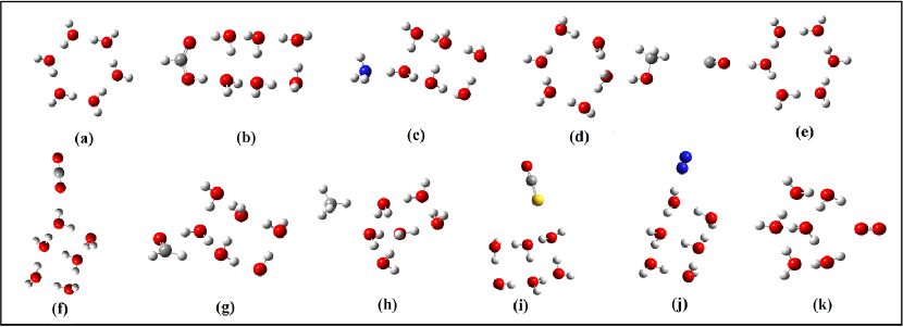
Figure S1: Optimized structures of (a) pure water, (b) $\rm{H_{2}O-HCOOH}$, (c) $\rm{H_{2}O-NH_{3}}$, (d) $\rm{H_{2}O-CH_{3}OH}$, (e) $\rm{H_{2}O-CO}$, (f) $\rm{H_{2}O-CO_{2}}$, (g) $\rm{H_{2}O-H_{2}CO}$, (h) $\rm{H_{2}O-CH_{4}}$, (i) $\rm{H_{2}O-OCS}$, (j) $\rm{H_{2}O-N_{2}}$, and (k) $\rm{H_{2}O-O_{2}}$ clusters with a $6:1$ concentration ratio.

While the outcome of this comparison will be discussed later in the text, here we anticipate that the 4H₂O cluster in the c-tetramer configuration will be chosen as water ice unit. To investigate the effect of impurities, a number of impurity molecules have been added in order to obtain the desired ratio, as shown in Table 2. For example, in order to get 2:1 ratio of water:impurity(x), we considered $4$ water molecules hooked up with $2$ ‘$\rm{x}$’ molecules. However, for some systems, to have more realistic features of the water cluster, we needed to consider more water molecules. Since it is known that the water ice clusters containing six $\rm{H_{2}O}$ molecules are the form of all natural snow and ice on Earth ⁶⁸, we also present a case with six H₂O molecules together as a unit (see Figure S1 in the Supporting Information, SI). The cyclic hexamer (chair) configuration of the water cluster containing six $\rm{H_{2}O}$ has been found the most stable ¹⁹, and considered in our calculations.

Table 2: Ice mixture composition details.

H2O:X	Total no.	No. of	No. of
	of molecules	water molecules	pollutant molecules
1:0.25	5	4 (80.0%)	1 (20.0%)
1:0.50	6	4 (66.7%)	2 (33.3%)
1:0.75	7	4 (57.1%)	3 (42.9%)
1:1.00	8	4 (50.0%)	4 (50.0%)

Notes. Contributions in percentage are provided in the parentheses.

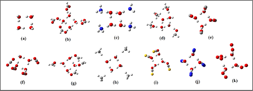
Figure 1: Optimized structures for (a) pure water and for the $4:4$ concentration ratio: (b) $\rm{H_{2}O-HCOOH}$, (c) $\rm{H_{2}O-NH_{3}}$, (d) $\rm{H_{2}O-CH_{3}OH}$, (e) $\rm{H_{2}O-CO}$, (f) $\rm{H_{2}O-CO_{2}}$, (g) $\rm{H_{2}O-H_{2}CO}$, (h) $\rm{H_{2}O-CH_{4}}$, (i) $\rm{H_{2}O-OCS}$, (j) $\rm{H_{2}O-N_{2}}$, (k) $\rm{H_{2}O-O_{2}}$ clusters.

In Figure 1a, we present the optimized water clusters for the c-tetramer configuration. The same structure was considered by Ohno et al. ¹⁹ and others ⁶⁹, ⁷⁰, ⁷¹. Since four H atoms are available for interacting with the impurities by means of hydrogen bond, in our calculations we can reach up to a $1:1$ ratio between the water and the impurity (i.e., we can reach up to 50% concentration of the impurity in the ice mixture).

In order to understand the effect of impurities on the band strengths of the four fundamental bands considered, we have calculated the area under the curve for each band for different mixtures of pure water and pollutants. The band strength has then been derived using the following relation (introduced in Bouwman et al. ²⁰ and Öberg et al. ²¹):

$$A_{H_{2}O:x=1:y}^{band}=\int_{band}I_{H_{2}O:x=1:y}\times\frac{A_{band}^{H_{2}O}}{\int_{band}I_{H_{2}O}},$$ (1)

where $A_{H_{2}O:x}^{band}$ is the calculated band strength of the vibrational water mode in the $1:y$ mixture, $I_{H_{2}O:x=1:y}$ is its integrated area, $A_{band}^{H_{2}O}$ is the band strength of the water modes available from the literature, and $\int_{band}I_{H_{2}O}$ is the integrated area under the vibrational mode for pure water ice. The experimental absorption band strengths of the three modes of pure water ice are taken from Gerakines et al. ²², who carried out measurements with amorphous water at $14$ K. The adopted values are $2\times 10^{-16}$, $1.2\times 10^{-17}$, $3.1\times 10^{-17}$ $\mathrm{cm\ molecule^{-1}}$, for the bulk stretching ($3280$ cm^-1), bending ($1660$ cm^-1), and libration mode ($760$ cm^-1), respectively. Our ab-initio calculations refer to the temperature at $0$ K. For the calculation of the band strengths, we are considering the strongest feature of that band. Since for the free-OH stretching mode no experimental values exist, we consider the result $A_{free-OH}^{H_{2}O}=2.09\times 10^{-17}$ and $2.52\times 10^{-17}$ $\mathrm{cm\ molecule^{-1}}$ for the c-tetramer and hexamer water clusters, respectively.

2.1 Computational details

As already mentioned, quantum-chemical calculations have been performed to evaluate the changes of the absorption features of four different fundamental modes, namely, (i) libration, (ii) bending, (iii) bulk stretching, and (iv) free-OH stretching of water in the presence of impurities (CO, $\rm{CO_{2}}$, $\rm{CH_{3}OH}$, $\rm{H_{2}CO}$, HCOOH, $\rm{CH_{4}}$, NH₃, OCS, $\rm{N_{2}}$, and $\rm{O_{2}}$). High-level quantum chemical calculations (such as CCSD(T) method and hybrid force field method) are proven to be the best suited for reproducing the experimental data ^{72, 73}. However, due to the dimension of our targeted species, these levels of theory are hardly applicable.

As already anticipated, different DFT functionals have been tested. Most computations have been carried out using the B3LYP hybrid functional ^{74, 75} in conjunction with the 6-31G(d) basis set (Gaussian 09 package ⁷⁶). Some test computations have also been performed by using the B2PLYP double-hybrid functional ⁷⁷ in conjunction with the the m-aug-cc-pVTZ basis set ⁷⁸, in which the $d$ functions have been removed on hydrogen atoms (maug-cc-pVTZ-$d$H). In this case, harmonic force fields have been obtained employing analytic first and second derivatives ⁷⁹ available in the Gaussian 16 suite of programs ⁸⁰. The reliability and effectiveness of this computational model in the evaluation of vibrational frequencies and intensities have been documented in several studies (see, for example, ref. 81). We have also performed anharmonic calculations (at the B3LYP/6-31G(d) level) for the H₂O-CO and H₂O-NH₃ systems in order to check the effect of anharmonicity on the band strength profiles of the four water fundamental modes.

The spectral features of the astrophysical ices can be altered in both active (direct) and passive (bulk) ways. Following a consolidated practice ⁸², to include the passive contribution of the bulk ice on the spectral properties of the ice mixtures considered, we embedded our explicit cluster in a continuum solvation field to represent local effects on the ice mixture. To this end, we resorted to the integral equation formalism (IEF) variant of the Polarizable Continuum Model (PCM) ⁸³. The solute cavity has been built by using a set of interlocking spheres centered on the atoms with the following radii (in Å): $1.443$ for hydrogen, $1.925$ for carbon, $1.830$ for nitrogen, and $1.750$ for oxygen, each of them scaled by a factor of $1.1$, which is the default value in Gaussian. For the ice dielectric constant, that of bulk water ($\varepsilon=78.355$) has been used, although any dielectric constant larger than about $30$ would lead to very similar results. In addition, we have also performed QM/MM geometry optimizations of a pure water cluster containing 4 H₂O molecules, in which all but one molecule at the square vertexes were put in the MM layer (see Figure 2, left panel). A pure water cluster system containing 20 H₂O molecules has also been considered. For this, we started from the coordinates of the full QM optimization and selected two alternative sets of four innermost molecules at the center of the cluster with a complete hydrogen bond network (determined with a geometric criterion ⁸⁴) with first neighbor water molecules; the remaining 16 molecules were described at the MM level (see Figure 2, right panel). All QM/MM ⁸⁵ calculations were carried out with the Gaussian 16 ⁸⁰ code (rev. C01) using the hybrid B3LYP functional in conjunction with the 6-31 G(d) basis set. Atom types and force field parameters for water molecules in the MM layer were assigned according to the SPC-Fw flexible water model ⁸⁶; the choice was driven by (i) the necessity for a flexible, 3-body classical water model and (ii) the accuracy with which the selected model reproduced ice I_h properties. Solvent effects were mimicked by using PCM ⁸⁷. The vibrational analysis results from QM/MM calculations are provided in Tables S10, S11, and S12 in the SI.

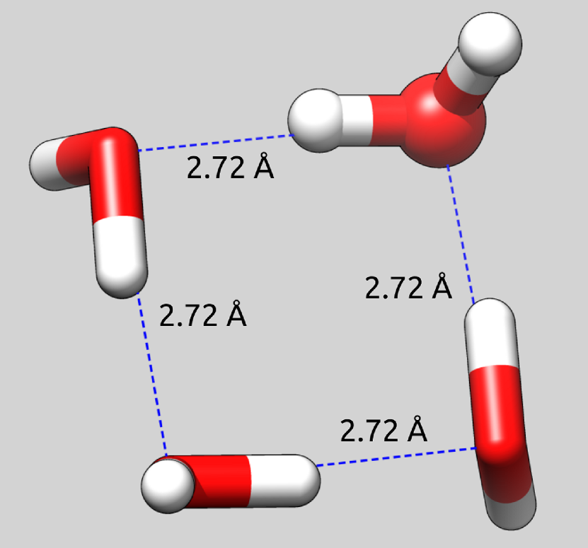
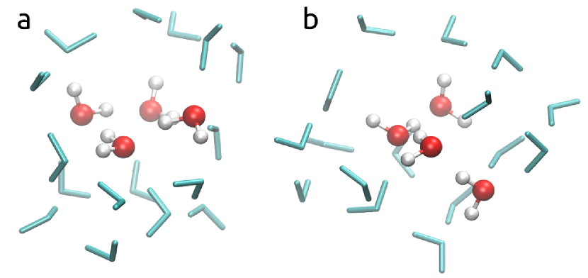
Figure 2: Left: 4 water system; the single QM water molecule is depicted in ball and stick representation and the 3 MM molecules in licorice representation; O-H distances are indicated too. It is to be noted that the four H₂O can be considered equivalent, Right: Innermost water molecules described at QM level (ball and stick) and surrounding molecules described at MM level (lines) for the 20H₂O system. (a) Configuration 1. (b) Configuration 2.

3 Experimental Methods

Literature laboratory data are here used whenever possible to constrain simulations ^{20, 21}. In the cases of formic acid, ammonia, and methanol in water ice, new experiments have been performed using the high vacuum (HV) Portable Astrochemistry Chamber (PAC) at the Open University (OU) in the United Kingdom. A detailed description of the system is reported elsewhere ⁸⁸. Briefly, the main chamber is a commercial conflat flange cube (Kimball Physics Inc.) connected to a turbo molecular pump (300 l/s), a custom made stainless steel dosing line through an all metal leak valve, a cold finger of a closed-cycle He cryostat (Sumitomo Cryogenics) and two ZnSe windows suitable for IR spectroscopy. During operation, the base pressure in the chamber is in the 10^-9 mbar range, and the base temperature of the cold finger is 20 K. In thermal contact with the cryostat, the substrate is a ZnSe window (20 mm x 2 mm). A DT-670 silicon diode temperature sensor (LakeShore Cryotronics) is connected to the substrate to measure its temperature, while a Kapton flexible heater (Omegalux) is used to change its temperature. Diode and heater are both connected to an external temperature controller (Oxford Instruments).

Gaseous samples were prepared and mixed in a pre-chamber (dosing line) before being dosed into the main chamber through an all metal leak valve. A mass-independent pressure transducer was used to control the amount of gas components mixed in the pre-chamber. Chemicals were purchased at Sigma-Aldrich with the highest purity available [HCOOH ($>$95%), NH₃ (99.95%), and CH₃OH (99.8%)]. Ices were grown $insitu$ by direct vapour deposition onto the substrate at normal incidence via a 3 mm nozzle that is 20 mm away from the sample. Infrared spectroscopy was performed in transmission using a Fourier Transform infrared (FTIR; Nicolet Nexus 670) spectrometer with an external Mercury cadmium telluride (MCT) detector. A background spectrum comprising 512 co-added scans was acquired before deposition at 20 K and used as reference spectrum for all the spectra collected after deposition to remove all the infrared signatures along the beam pathway that were not originated by the ice sample. Each IR spectrum is a collection of 256 co-added scans. The IR path was purged with dry compressed air to remove water vapour.

4 Results and Discussions

In this section, first of all, the pure water ice will be addressed in order to establish the best compromise between accuracy and computational cost for the description of the water ice unit cell. To this aim, we will resort on the comparison with experiment. Then, we will move to the ice containing impurities. To further proceed with the validation of our protocol, water ice containing HCOOH, NH₃, CH₃OH, CO, and CO₂ as impurities will be investigated, thus exploiting the comparison between experiment and computations. This will also involve, as mentioned above, new measurements. Finally, in the last part, our protocol will be extend to the study of water ices with H₂CO, CH₄, N₂, and O₂ as impurities.

4.1 Part 1. Validation

4.1.1 Band strength of pure water

In Table 3, the water band positions obtained with different methods and different sizes of the water cluster are compared with experimental data. Since computations provide several frequencies corresponding to a single mode of vibration, for the sake of comparison, we have reported the computed frequencies of the four fundamental modes after convolving them with a Gaussian function with an adequate width ⁸⁹ (all transition frequencies are collected in the Appendix, Table A1). The comparison of Table 3 is graphically summarized in Figure 3. The left panel shows the average deviation of the band position of three fundamental modes of water (libration, bending, and stretching) from the experimental counterpart ²². It is interesting to note that the band positions obtained using the tetramer configuration and the B3LYP/6-31G(d) level of theory provides the best agreement. The right panel shows the average deviation of the band strengths from experiments. QM/MM calculations for the 20 water-molecule cluster (as described in the computational details) show the minimum deviation from experimental data. The results obtained for the tetramer configuration, both at the B3LYP and B2PLYP level, also provide small deviations. Based on the results of the comparison carried out, the B3LYP/6-31G(d) level of theory and the tetramer configuration have been found to be a suitable combination to describe the water cluster with a limited computational cost.

Table 3: Absorption band strengths and band positions (within parentheses; in cm^-1) of pure water ice.

Vibration	Experiment	Computed values in cm molecule-1 and band position in cm-1
mode	Gerakines et al. 22	Dimer	c-Tetramer	c-Hexamar (chair)	Octamer (cube)
		B3LYP-631G(d)	B3LYP-631G(d)	B3LYP-631G(d)	B3LYP-631G(d)
Libration	$3.1\times 10^{-17}$ (760)	$2.70\times 10^{-17}(670)$	$2.40\times 10^{-17}(733)$	$1.17\times 10^{-16}(870)$	$1.27\times 10^{-17}(848)$
Bending	$1.2\times 10^{-17}$ (1660)	$2.23\times 10^{-17}(1710)$	$4.18\times 10^{-17}(1714)$	$4.62\times 10^{-17}(1730)$	$6.85\times 10^{-17}(1717)$
Stretching	$2.0\times 10^{-16}$ (3280)	$8.27\times 10^{-17}(3540)$	$3.11\times 10^{-16}(3298)$	$5.53\times 10^{-16}(3220)$	$3.89\times 10^{-16}(3320)$
Free-OH	$-$	$1.35\times 10^{-17}(3810)$	$2.10\times 10^{-17}(3775)$	$2.52\times 10^{-17}(3780)$	$1.52\times 10^{-17}(3788)$
Vibration	Experiment	Computed values in cm molecule-1 and band position in cm-1
mode	Gerakines et al. 22	c-Tetramer	1H2O(QM)+3H2O(MM)	4H2O(QM)+16H2O(MM)
		B2PLYP/m-aug-cc-pVTZ	B3LYP-631G(d)	B3LYP-631G(d)
Libration	$3.1\times 10^{-17}$ (760)	$3.94\times 10^{-17}(714)$	$7.91\times 10^{-17}(669)$	$4.9\times 10^{-17}(720)$
Bending	$1.2\times 10^{-17}$ (1660)	$2.93\times 10^{-17}(1635)$	$2.37\times 10^{-17}(1431)$	$1.88\times 10^{-17}(1426)$
Stretching	$2.0\times 10^{-16}$ (3280)	$2.97\times 10^{-16}(3477)$	$2.68\times 10^{-17}(3593)$	$1.76\times 10^{-16}(3565)$
Free-OH	$-$	$2.40\times 10^{-17}(3865)$	$6.24\times 10^{-18}(3797)$	$2.52\times 10^{-17}(3636)$

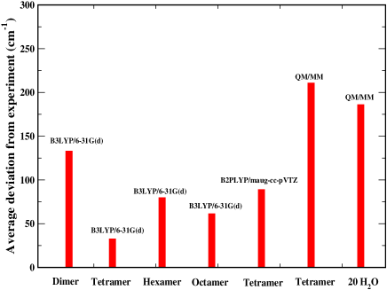
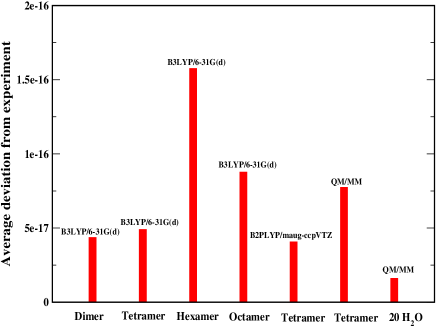
Figure 3: Deviation of computed band positions (left panel) and band strengths (right panel) from experiments.

In the following sections, the results for water ice with HCOOH and NH₃ as impurities are first reported and discussed, thereby exploiting the outcomes of new experiments. Then, we move to the CH₃OH-H₂O ice for which new experimental results have been obtained. For the last two cases addressed, namely CO-H₂O and CO₂-H₂O, the experimental data for the comparison have been taken from the literature. Unless otherwise stated, we use the c-tetramer configuration for the rest of our calculations.

4.1.2 HCOOH ice

Infrared spectra were measured for various mixtures of H₂O and HCOOH ice deposited at $20$ K, as explained in the experimental details section (see Section 3). These, normalized with respect to the O-H stretch, are shown in Figure 4a. A minor contamination due to CO₂ was detected in some experiments. In all experiments, the amount of CO₂ deposited in the ice was found to be between 1000 and more than 100 times less abundant than H₂O and HCOOH, respectively. Therefore, we do not expect that the CO₂ contamination affects the recorded IR spectra profiles.

The mixture ratios were determined from the fit of the the spectrum of a selected mixture, the measurement of the area of the water band at $3333.33$ cm^-1 (3.00 $\mu$m), and the comparison with the pure water counterparts. For HCOOH, the absorption area is measured at 1700 cm^-1. In fact, HCOOH has the strongest mode at $1694.92$ cm^-1 ($5.90$ $\mu$m) which corresponds to its C=O stretching mode. But the feature overlaps with the position of the OH bending mode of solid water at $1666.67$ cm^-1 ($6.00$ $\mu$m). The contribution from the water bending mode at $\sim$1700 cm^-1 has been subtracted from the total area before the band strength mentioned above being used to calculate the amount of HCOOH in the ice mixture. The band strengths used here are $2.0\times 10^{-16}$ for H₂O ²² and $6.7\times 10^{-17}$ for HCOOH ^{90, 24}. Another relatively weaker mode of HCOOH at $1388.89$ cm^-1 ($7.20$ $\mu$m) was also considered because the corresponding region is free from interfering transitions ²⁴. As seen in Figure 4a, the HCOOH:H₂O ratios cover the 0.05 to 3.46 range. In this respect, it is worthwhile noting that the abundances of solid phase HCOOH in the interstellar ices vary between 1% to 5% with respect to the $\rm{H_{2}O}$ ice ⁹¹.

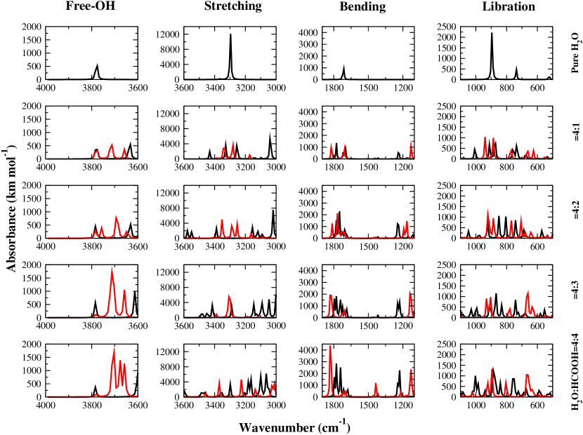
Figure A4: Absorption spectra of the four modes for water ice for the five measured compositions, ranging from pure water ice (top) to 4:4 H₂O-HCOOH mixture (bottom). Black line represent the absorbance spectra of various concentration of H₂O-HCOOH, where HCOOH is used as hydrogen bond donor and for red line HCOOH is used as hydrogen bond acceptor.

Moving to the computational study, Figure 1b shows how the HCOOH molecules are bonded to the water molecules to form the $4:4$ H₂O-$\rm{HCOOH}$ mixture used in our calculations. In the Appendix, the absorption band profiles of the H₂O-HCOOH clusters with different impurity concentrations are shown (see Figure A4). The transition frequencies and the corresponding strongest intensity values, obtained at the B3LYP/6-31G(d) level, are given in the Appendix (see Table A2). Calculations have also been carried out using the B2PLYP functional, the results being summarized in Tables S1, S2, S3, S4, and S5 in the SI.

To investigate how the band strength varies with impurity concentrations, the data are fitted with a linear function A_eff = a$\cdot$[X] + b, where X = HCOOH, NH₃, $\rm{CH_{3}OH}$, CO, $\rm{CO_{2}}$, $\rm{H_{2}CO}$, CH₄, OCS, N₂, and O₂. The coefficient ‘a’ provides the information whether the band strength increases or decreases by increasing the concentration of X, [X], and the coefficient ‘b’ indicates the band strength of the vibration mode in the absence of impurities. The fitting coefficients, for all impurity considered, are provided in Table 4. In Figure 5a, the band strength profile as a function of the concentration of HCOOH is shown.

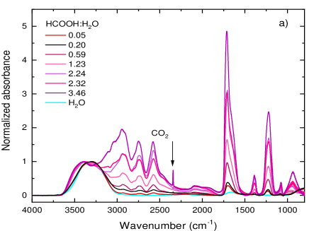
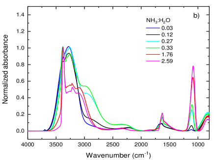
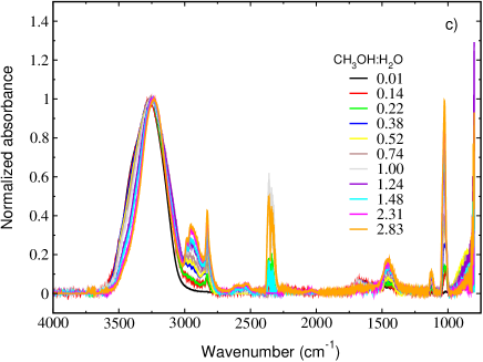
Figure 4: (a) IR spectra for different HCOOH:H₂O ice mixtures deposited at T$=20$ K. (b) IR spectra for different NH₃:H₂O ice mixtures deposited at T$=20$ K. (c) IR spectra of different CH₃OH:H₂O ice mixtures deposited at T$=30$ K. The color legend is explained in the insets. All IR spectra are normalized with respect to the O-H stretching band.

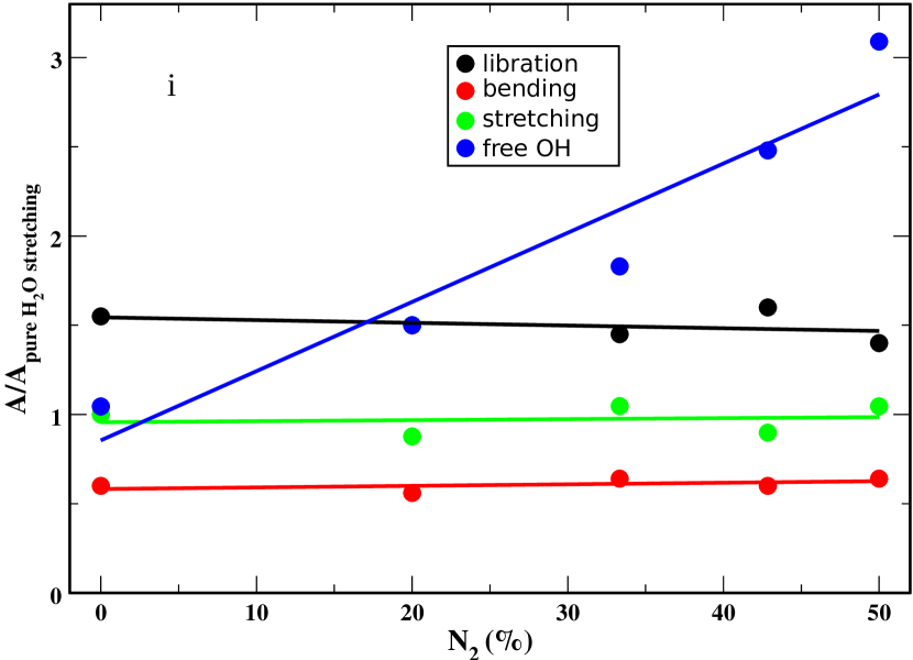
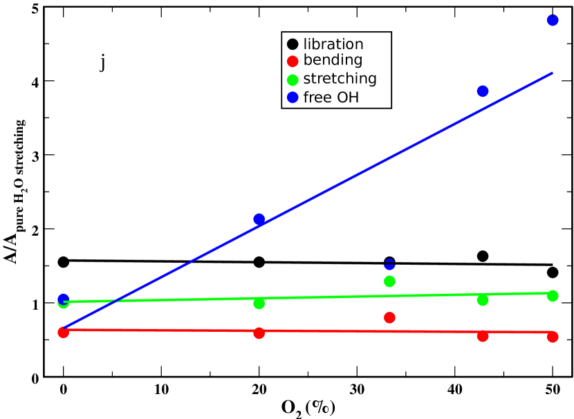
Figure 5: Band strengths of the four fundamental vibration modes of water for (a) $\rm{H_{2}O-HCOOH}$, (b) $\rm{H_{2}O-NH_{3}}$, (c) $\rm{H_{2}O-CH_{3}OH}$, (d) $\rm{H_{2}O-CO}$, (e) $\rm{H_{2}O-CO_{2}}$, (f) $\rm{H_{2}O-H_{2}CO}$, (g) $\rm{H_{2}O-CH_{4}}$, (h) $\rm{H_{2}O-OCS}$, (i) $\rm{H_{2}O-N_{2}}$, and (j) $\rm{H_{2}O-O_{2}}$ clusters with various concentrations. The water c-tetramer configuration was used for pure water.

4.1.3 NH₃ ice

Most of the intense modes of ammonia overlap with the dominant features due to water and silicates. However, when ammonia is mixed with $\rm{H_{2}O}$ ice, it forms hydrates that show an intense mode at $2881.84$ cm^-1 ($3.47$ $\mu$m) ¹⁶, which lies in a relative clear region. Another characteristic feature of ammonia is the umbrella mode at $1111.11$ cm^-1 ($9.00$ $\mu$m), which is relatively intense, but it often overlaps with the $\rm{CH_{3}}$ rocking mode of methanol, thus leading to an overestimation of the abundance of ammonia.

In this work, infrared spectra were recorded for various mixing ratios of H₂O-NH₃ ice deposited at 20 K. The IR spectra, normalized with respect to the most intense bend (i.e. the O-H stretching mode), are shown in Figure 4b. Mixing ratios were derived by measuring the areas of the selected bands for H₂O band (at 2220 cm^-1) ⁹² and for NH₃ (umbrella mode band at 1070 cm^-1) ⁹³, with a procedure analogous to that introduced in the previous section for HCOOH.

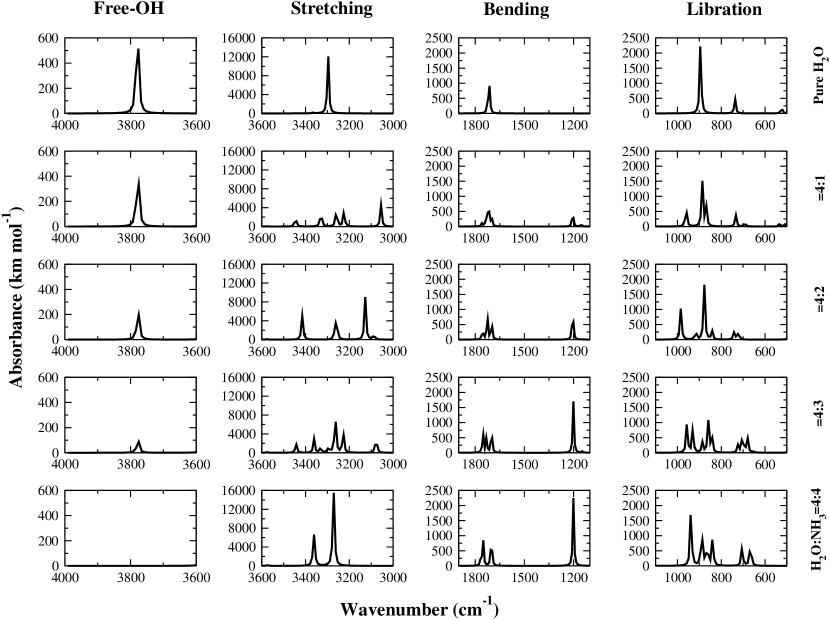
Figure A5: Absorption spectra of the four modes for water ice for the five measured compositions, ranging from pure water ice (top) to 4:4 H₂O-NH₃ mixture (bottom).

Figure 1c shows the optimized geometry of the H₂O-$\rm{NH_{3}}$ system with a $4:4$ ratio as obtained from our quantum-chemical calculations. In the Appendix, Figure A5 depicts the absorption band profiles of H₂O-$\rm{NH_{3}}$ mixtures with various concentrations. The transition frequencies and the corresponding intensity values are provided in the Appendix as well (see Table A2). The vibrational analysis has also been carried out at a higher level of theory, thereby using the B2PLYP functional. The results are reported in Tables S6, S7, S8, and S9 in the SI. Figure 5b shows the band strengths as a function of the concentration of the impurity under consideration, i.e. NH₃.

4.1.4 Comparison between experiment and simulations

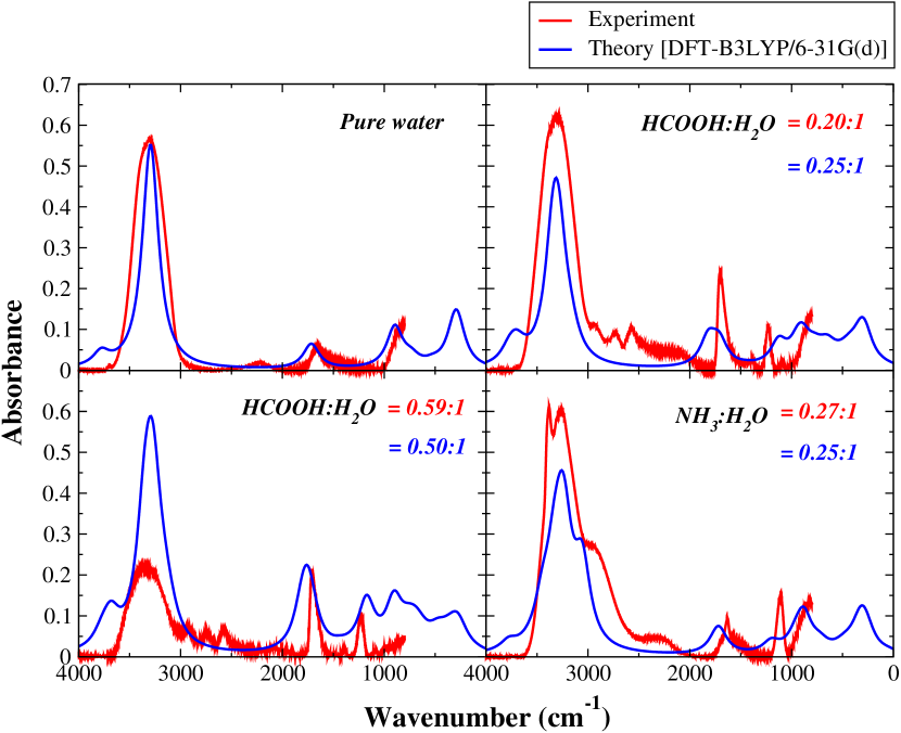
Figure 6: Comparison of computed and experimental IR spectra (0 - 4000 cm^-1) for pure water as well as water with HCOOH and NH₃ as impurities. We have used harmonic frequencies for the computed spectra and the intensity is scaled with a factor 1000 to have best match with the experimental one.

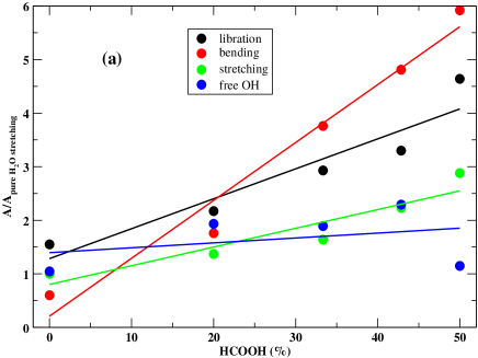
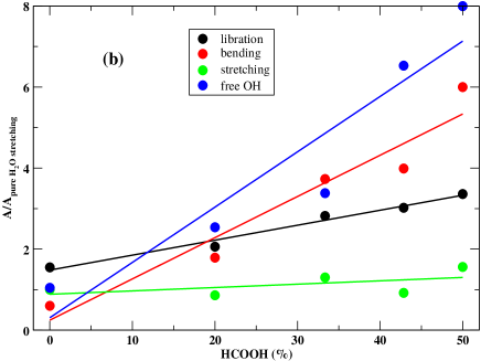
Figure A2: Band strength for H₂O-HCOOH mixtures: (a) HCOOH as hydrogen bond donor, and (b) HCOOH as hydrogen bond acceptor.

In Figure 6, the comparison between experimentally obtained spectra and our computed spectra for pure water, H₂O-HCOOH mixture, and H₂CO-NH₃ mixture is shown. We note a good agreement between experimental and theoretical absorption spectra. Figure 7 shows the comparison between the experimental (dotted lines) and theoretical (solid and dashed lines) band strengths of the four water bands as a function of the concentration of HCOOH and NH₃. From Figure 7, it is evident that the experimental strength of the libration and bending modes increases by increasing the concentration of HCOOH. On the contrary, the strength of the stretching and free OH modes shows a decreasing trend. These behaviors should be compared with the B2PLYP/mug-cc-pVTZ (dashed) and B3PLYP/6-31G(d) (solid) trends. For the libration and bending band strength profiles, there is a qualitative agreement with experiments. In the case of the stretching and free OH modes, theoretical band strength profiles deviate from experimental work. The lack of experimental data in the 3600-4000 cm^-1 range (see Figure 4a) may have contributed to this disagreement. Concerning the comparison of the two levels of theory, it is noted that there is a rather good agreement. In case of H₂O-HCOOH mixture, HCOOH can act as both hydrogen bond donor and hydrogen bond acceptor. We considered both the interactions and noted that, if we consider HCOOH as H-bond acceptor, the band strength of three modes (libration, bending, and stretching) are lower with respect to case where HCOOH was treated as H-bond donor. But in the case of the free-OH mode, the band strength slope increases (See Figure A2 in the Appendix).

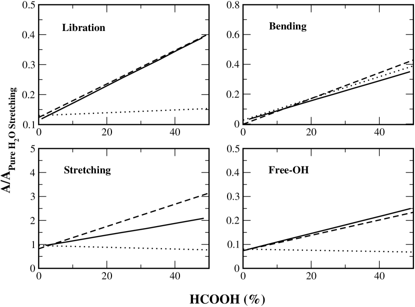
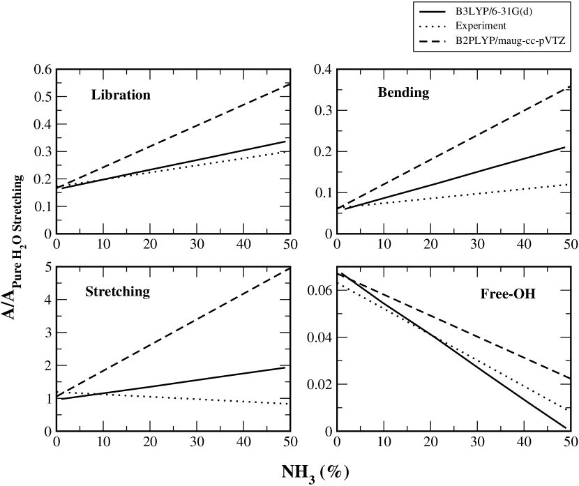
Figure 7: Comparison between the calculated and experimental band strength profiles with various concentration of HCOOH and NH₃.

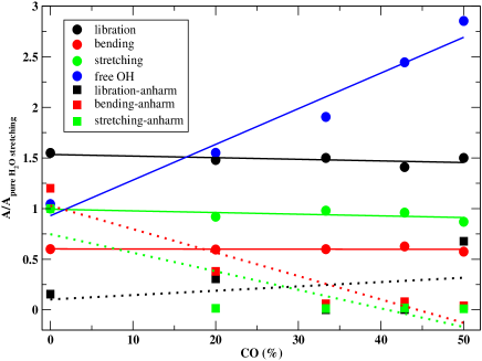
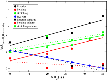
Figure A1: The filled circles are the data points where we considered harmonic frequencies and the corresponding fitted profiles are the solid lines. Solid filled squares represent the data sets where we considered anharmonic frequencies and the corresponding fitted results are the dotted lines.

Moving to ammonia, the experimental data of Figure 7 show that the band strength of the free-OH stretching mode nearly vanishes when a 50% concentration of the impurity (NH₃) is reached. This feature interestingly supports our calculated spectra shown in the Appendix (see Figure A5 last panel). Libration and bending modes have, instead, an opposite trend, with the band strength increasing by increasing the concentration of NH₃. The band strength of the stretching mode shows a slightly decreasing trend with the concentration of NH₃. From the inspection of Figure 7 it is evident that both sets of theoretical results (B3LYP and B2PLYP) are in reasonably good agreement with experimental data for the libration, bending, and free-OH modes. Interestingly, the results obtained using the lower level of theory are in better agreement with experiments. In Figure A1 (in the Appendix), the comparison of band strengths evaluated using (a) harmonic and (b) anharmonic calculations is shown. To investigate the effect of anharmonicity on the band strengths, we have only considered fundamental bands in the 0 to 3600 cm^-1 frequency range. From our experimental study on the H₂O-NH₃ system, as already mentioned, we obtained an increasing trend of the band strength for the libration, bending, and stretching modes with the increase in concentration of NH₃, whereas the band strength decreases for the free OH mode and tends to zero with 50% concentration of NH₃. When using harmonic calculations for all four fundamental modes, trends similar to what obtained from experiment were found. But, if we consider anharmonic calculations, only the behavior of the stretching mode is well reproduced. All other modes deviate from the experimental results. While not claiming that harmonic calculations are better than the anharmonic ones, this comparison seems to suggest that the former show a better error compensation. A similar outcome has been obtained for the H₂O-CO system and will be briefly addressed later in the text.

Based on the comparisons discussed above, the B3LYP/6-31G(d) level of theory provides reliable results. Therefore, it has been employed in the following investigations. First of all, the comparison between computed and experimental band strengths for the H₂O-CH₃OH, CO-H₂O, and CO₂-H₂O mixtures will be considered to further support its suitability.

4.1.5 CH₃OH ice

In this work, the effect of the CH₃OH concentration on the band profiles of water ice has been experimentally investigated. In the case of methanol, CO₂ gas is still present in the system (i.e., outside the vacuum chamber) in quantities that vary in time causing negative and/or positive contributions to CO₂ gas-phase absorption features with respect to the background spectrum, as evident in Figure 4c at $\sim$2340 cm^-1. Such contamination is most likely due to the dosing line, but its negligible amount should not affect the final results. Figure 4c shows the experimental absorption spectra for various CH₃OH-H₂O ice mixtures deposited at T$=30$ K. The spectra are normalized to 1 with respect to the maximum of the O-H stretch band.

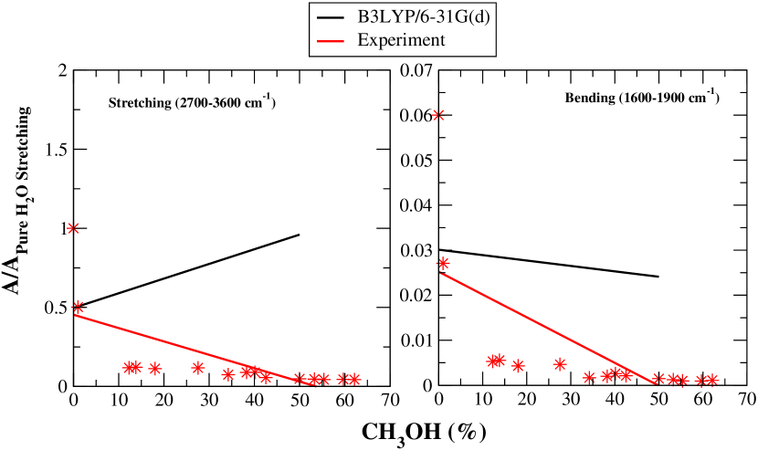
Figure 8: Comparison between calculated and experimental band strength profiles as a function of CH₃OH concentration. Stars represent the experimental data points.

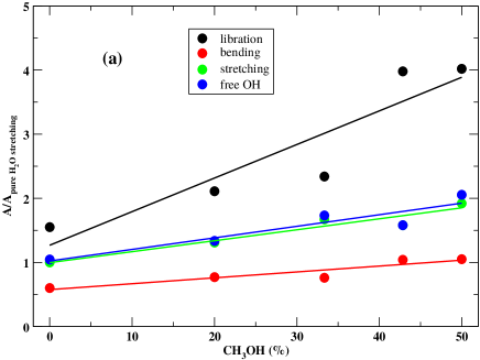
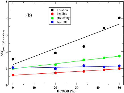
Figure A3: Band strength for H₂O-CH₃OH mixtures: (a) CH₃OH as hydrogen bond donor, and (b) CH₃OH as hydrogen bond acceptor.

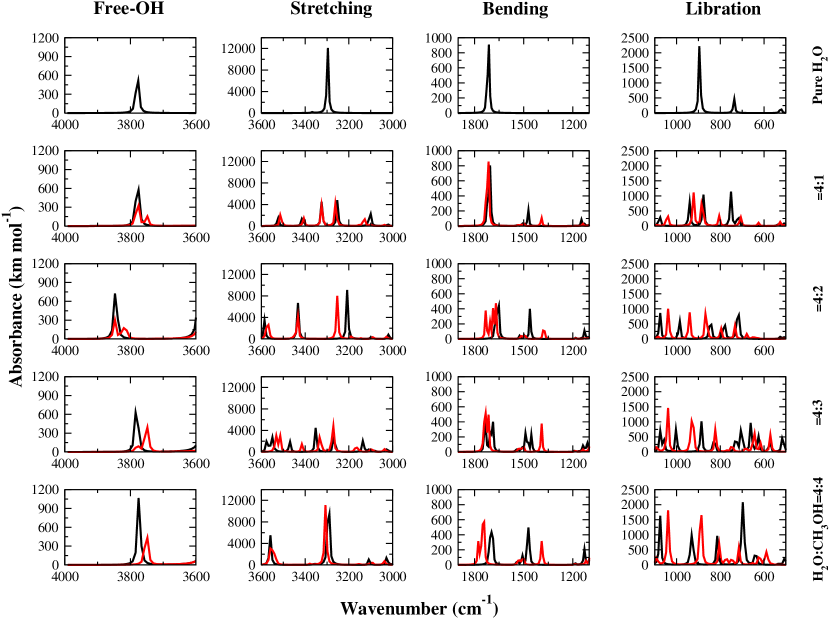
Figure A6: Absorption spectra of the four modes for water ice for the five measured compositions, ranging from pure water ice (top) to 4:4 H₂O-CH₃OH mixture (bottom). Black line represent the absorbance spectra of various concentration of H₂O-CH₃OH, where CH₃OH is used as hydrogen bond donor and for red line CH₃OH is used as hydrogen bond acceptor.

Figure 1d shows the optimized structure of the $\rm{H_{2}O}$-$\rm{CH_{3}OH}$ mixture with a $4:4$ concentration ratio. It is noted that a weak hydrogen bond is expected to be formed. The simulated IR spectra for different concentrations are shown in Figure A6 (in the Appendix). Peak positions, integral absorption coefficients, and band assignments for various H₂O-CH₃OH mixtures are collected in Table A2 in the Appendix. The computed band strengths as a function of different concentrations are shown in Figure 5c. The computed strength of the bending mode gradually increases with $\rm{CH_{3}OH}$ concentration (see Figure 8; right panel), which is in qualitative agreement with the experimental results ⁸⁸. In case of the stretching mode, computationally, a slight increasing trend of the band strength is noted, whereas experimental results show an opposite trend (see Figure 8; left panel). Because of the lack of experimental spectra, we cannot compare the band strength of the libration and free OH modes. In case of H₂O-CH₃OH mixtures, methanol can act as both hydrogen bond donor and hydrogen bond acceptor. We considered both possibilities and found that if we consider methanol as hydrogen bond donor, the band strength of all four modes show an increasing trend. On the other hand, if we consider methanol as hydrogen bond acceptor, the band strengths of three modes, namely libration, bending, and stretching, present trends similar to the previous case (where methanol acts as hydrogen bond donor), while the free-OH band shows a less pronounced behavior (see Figure A3 in the Appendix).

4.1.6 CO ice

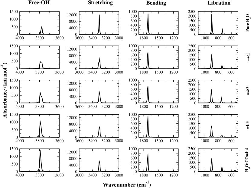
Figure A7: Absorption spectra of the four modes for water ice for the five measured compositions, ranging from pure water ice (top) to 4:4 H₂O-CO mixture (bottom).

Figure 1e depicts the H₂O-CO optimized structure with a $4:4$ concentration ratio: the four CO molecules interact with the H atoms of the water molecules not involved in the hydrogen bond (interaction of the O atom of CO with the hydrogen atom of water). However, for the H₂O-CO system, the interaction can take place through both O and C of CO with the hydrogen atom of H₂O ⁹⁴. We have considered both types of interaction and evaluated their effects on the band strengths. However we did not find any significant difference. Thus, we only discuss the band strength of the H₂O-CO mixture with the interaction on the O side of CO. For the sake of completeness, it should be mentioned that there is also another type of interaction, which occurs between the $\pi$ bond of CO and one water-hydrogen, and it gives rise to a T shaped complex ⁹⁵. However, according to a computational study by Collings et al. ⁹⁵, this has a negligible effect on IR vibrational bands. As a consequence we have not investigated in detail this kind of complex. The simulated IR absorption spectra of the four fundamental vibrational modes for various compositions are shown in the Appendix (see Figure A7). The four fundamental frequencies of water ice change significantly by increasing the concentration of CO. The most intense peak positions and the corresponding integral abundance coefficients for different H₂O-CO mixtures are provided in the Appendix (see Table A2). In Figure 5d, the integrated intensities of water vibrational modes are plotted as a function of the CO concentration. It is noted that the strength of the libration, bending, and stretching modes decreases with the concentration of CO. The free OH mode shows instead a sharp increase of the band strength when increasing the CO concentration. In Table 4, the resulting linear fit coefficients are collected together with the available experimental values for H₂O-CO mixtures deposited at $15$ K ²⁰. It is noted that theoretical band strength slopes are in rather good agreement with experimental results ²⁰. For the H₂O-CO system, anharmonic calculations have also been carried out. While the band strengths of the bending and stretching modes have a similar trend as experimental data, a deviation is noted for the libration mode (see Figure A1 in the Appendix).

To check the effect of dispersion, B3LYP-D3/6-31G(d) calculations have been performed, with D3 denoting the correction for dispersion effects ⁹⁶. B3LYP-D3 calculations have been carried out for H₂O-CO, H₂O-CH₄, H₂O-N₂, and H₂O-O₂ systems. In Figure 9a, we have shown the comparison of the band strengths of different vibrational modes of water with and without the dispersion correction for the H₂O-CO system. The overall conclusion is that there is a good agreement with the experimental band strengths when dispersion effect is not considered. On the contrary, when the dispersion correction is included, our computed band strength profile shows a different trend. The libration and bending modes present a positive slope with the increase in impurity concentration, whereas experimental results show a negative slope. For the free OH mode, a slight increasing trend of the band strength is obtained, whereas the experimental band strength presents a sharp increase with the concentration of CO. The band strength of the stretching mode has a similar behaviour with dispersion and without dispersion, and in agreement with the experimental result ²⁰(see Figure 3). Thus, in summary, while we are not claiming that the dispersion effects are not important for the systems investigated, we have noted that neglecting them we obtain a consistent description of the experimental behaviour (probably due to a fortuitous errors compensation).

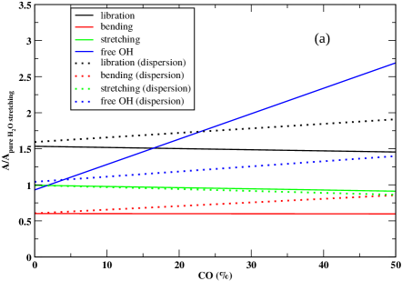
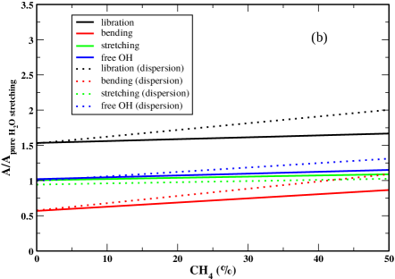
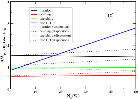
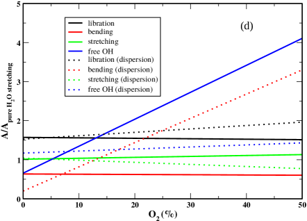
Figure 9: Comparison of the band strengths of the four fundamental modes of water for various mixtures of (a) H₂O-CO, (b) H₂O-CH₄, (c) H₂O-N₂, and (d) H₂O-O₂ by considering or not the dispersion effect.

Table 4: Linear fit coefficients for the $\rm{H_{2}O-X}$ (X = HCOOH, $\rm{NH_{3}}$, $\rm{CH_{3}OH}$, CO, $\rm{CO_{2}}$, $\rm{H_{2}CO}$, $\rm{CH_{4}}$, OCS, $\rm{N_{2}}$, and $\rm{O_{2}}$) mixtures.

Mixture	Vibrational	Linear coefficients
	mode	Constant	Slope
		[$\rm 10^{-16}$ cm $\rm molecule^{-1}$]	[$\rm 10^{-19}$ cm $\rm molecule^{-1}$]
H2O-$\rm{HCOOH}$	$\mathrm{\nu_{libration}}$	2.45 (0.26)a	132.73 (0.90)a
	$\mathrm{\nu_{bending}}$	0.58 (0.05)a	184.25 (14.40)a
	$\mathrm{\nu_{stretching}}$	1.80 (1.90)a	48.60 (-7.30)a
	$\mathrm{\nu_{free-OH}}$	0.20 (0.16)a	9.80 (-0.40)a
H2O-$\rm{NH_{3}}$	$\mathrm{\nu_{libration}}$	0.27 (0.34)a	6.11 (5.00)a
	$\mathrm{\nu_{bending}}$	0.09 (0.12)a	5.48 (2.20)a
	$\mathrm{\nu_{stretching}}$	1.90 (2.38)a	0.41 (-14.4)a
	$\mathrm{\nu_{free-OH}}$	0.21 (0.12)a	-4.21 (-2.1)a
H2O-$\rm{CH_{3}OH}$	$\mathrm{\nu_{libration}}$	0.25	10.0
	$\mathrm{\nu_{bending}}$	0.12	2.00
	$\mathrm{\nu_{stretching}}$	1.92	32.00
	$\mathrm{\nu_{free-OH}}$	0.26	2.65
H2O-CO	$\mathrm{\nu_{libration}}$	0.30 (0.30$\pm$0.02)20	-0.32 (-2.1$\pm$0.4)20
	$\mathrm{\nu_{bending}}$	0.12 (0.13$\pm$0.02)20	-0.016 (-1.0 $\pm$0.3)20
	$\mathrm{\nu_{stretching}}$	1.98 (2.0$\pm$0.1)20	-3.2 (-16$\pm$3)20
	$\mathrm{\nu_{free-OH}}$	0.18 (0.0)20	5.69 (1.2 $\pm$0.1)20
H2O-$\rm{CO_{2}}$	$\mathrm{\nu_{libration}}$	0.3 (0.32$\pm$0.02)21	2.07 (-3.2$\pm$0.4)21
	$\mathrm{\nu_{bending}}$	0.11 (0.14$\pm$0.01)21	0.12 (-0.5$\pm$0.2)21
	$\mathrm{\nu_{stretching}}$	2.02 (2.1$\pm$0.1)21	-0.22 (-22$\pm$2)21
	$\mathrm{\nu_{free-OH}}$	0.19 (0.0)21	10.02 (1.62$\pm$0.07)21
H2O-$\rm{H_{2}CO}$	$\mathrm{\nu_{libration}}$	0.26	5.73
	$\mathrm{\nu_{bending}}$	0.10	4.59
	$\mathrm{\nu_{stretching}}$	1.92	0.10
	$\mathrm{\nu_{free-OH}}$	0.13	16.53
H2O-$\rm{CH_{4}}$	$\mathrm{\nu_{libration}}$	0.31	0.53
	$\mathrm{\nu_{bending}}$	0.11	1.18
	$\mathrm{\nu_{stretching}}$	2.01	3.39
	$\mathrm{\nu_{free-OH}}$	0.20	0.52
H2O-$\rm{OCS}$	$\mathrm{\nu_{libration}}$	0.30	0.42
	$\mathrm{\nu_{bending}}$	0.11	0.23
	$\mathrm{\nu_{stretching}}$	1.96	2.18
	$\mathrm{\nu_{free-OH}}$	0.17	0.13
H2O-$\rm{N_{2}}$	$\mathrm{\nu_{libration}}$	0.31	-0.30
	$\mathrm{\nu_{bending}}$	0.12	0.17
	$\mathrm{\nu_{stretching}}$	0.12	0.11
	$\mathrm{\nu_{free-OH}}$	0.17	7.75
H2O-$\rm{O_{2}}$	$\mathrm{\nu_{libration}}$	0.31	-0.23
	$\mathrm{\nu_{bending}}$	0.12	-0.13
	$\mathrm{\nu_{stretching}}$	2.02	4.71
	$\mathrm{\nu_{free-OH}}$	0.13	13.80

Notes. Experimental values are provided in the parentheses. ^aThis work.

4.1.7 CO₂ ice

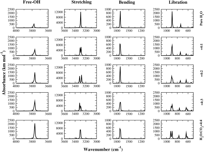
Figure A8: Absorption spectra of the four modes for water ice for the five measured compositions, ranging from pure water ice (top) to 4:4 H₂O-CO₂ mixture (bottom).

Figure 1f shows the optimized geometry of the $4:4$ mixture of H₂O:$\rm{CO_{2}}$. The absorption features of water ice for different $\rm{CO_{2}}$ concentrations are shown in the Appendix (see Figure A8). The most intense frequencies for the various H₂O-CO₂ mixtures are summarized in the Appendix as well (see Table A2). The trend of the band strength as a function of CO₂ concentrations is shown in Figure 5e. For the free-OH mode, a rapid increase with CO₂ concentration is noted, which is in good agreement with the experimental results by Öberg et al. ²¹. Computed band strengths of the libration and bending modes also increase by increasing the $\rm{CO_{2}}$ concentration, which is however in contrast with the available experimental data ²¹. The band strength of the bulk stretching mode decreases instead with $\rm{CO_{2}}$ concentration, in reasonable good agreement with the available experiments ²¹. FTIR spectroscopy of the matrix-isolated molecular complex H₂O-CO₂ shows that CO₂ does not form a weak hydrogen bond with H₂O ⁹⁷, but instead CO₂ destroys the bulk hydrogen bond network. This may cause a large decrease in the band strength of the bulk stretching mode, while the intermolecular O-H bond strength increases with the CO₂ concentration. Therefore, the disagreement between calculated and experimental band strengths could be thus due to the cluster size of water molecules. In Table 4, the resulting linear fit coefficients are reported, together with the available experimental values for the H₂O-CO₂ mixture deposited at $15$ K ²¹.

4.2 Part 2. Applications

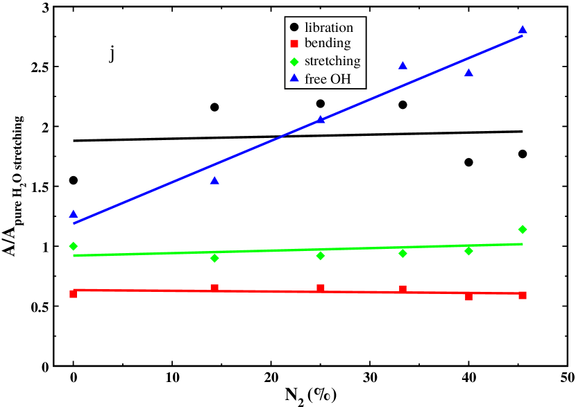
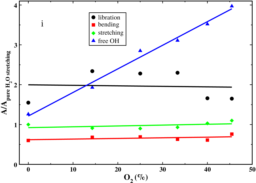
Figure S2: Band strengths of the four fundamental vibration modes of water for (a) $\rm{H_{2}O-HCOOH}$, (b) $\rm{H_{2}O-NH_{3}}$, (c) $\rm{H_{2}O-CH_{3}OH}$, (d) $\rm{H_{2}O-CO}$, (e) $\rm{H_{2}O-CO_{2}}$, (f) $\rm{H_{2}O-H_{2}CO}$, (g) $\rm{H_{2}O-CH_{4}}$, (h) $\rm{H_{2}O-OCS}$, (i) $\rm{H_{2}O-N_{2}}$, and (j) $\rm{H_{2}O-O_{2}}$ clusters with various concentrations. The water c-hexamer (chair) configuration gas been used for pure water.

The results discussed in previous sections suggest that the water c-tetramer structure together with harmonic B3LYP/6-31G(d) calculations are able to predict the experimental results presented here as well as literature data. Thus, to study the effect of other impurities ($\rm{H_{2}CO}$, CH₄, OCS, N₂, and O₂) on pure water ice, we have further exploited this methodology. Additionally, the effect of impurities on the band strengths of the four fundamental bands has also been studied by considering the c-hexamer (chair) structure and the corresponding results are provided in the SI (see Figure S2).

4.2.1 H₂CO ice

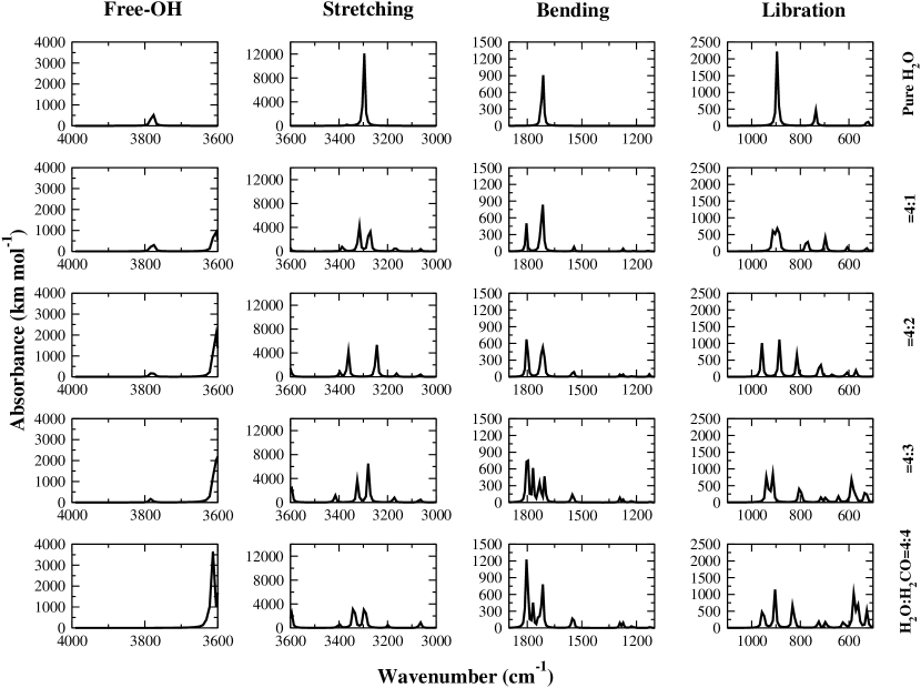
Figure A9: Absorption spectra of the four modes for water ice for the five measured compositions, ranging from pure water ice (top) to 4:4 H₂O-H₂CO mixture (bottom).

The strongest modes of formaldehyde ($\rm{H_{2}CO}$) lie at $1724.14$ cm^-1 ($5.80$ $\mu$m) and $1497.01$ cm^-1 ($6.68$ $\mu$m). Figure 1g depicts the optimized structure of the $4:4$ $\rm{H_{2}O-H_{2}CO}$ mixture. The desired ratio is attained upon formation of the hydrogen bond between the O atom of $\rm{H_{2}CO}$ and the dangling H atoms of $\rm{H_{2}O}$. The effect of formaldehyde on water IR spectrum is shown in the Appendix (see Figure A9). Frequencies, integral absorption coefficients, and mode assignments are reported in the Appendix as well (see Table A2). The band strength profiles as a function of the concentration of H₂O are shown in Figure 5f. Similar to the methanol-water mixture, all band strengths are found to increase with the concentration of formaldehyde, the free-OH stretching mode being the most affected.

4.2.2 CH₄ ice

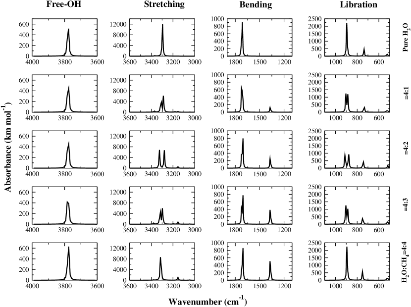
Figure A10: Absorption spectra of the four modes for water ice for the five measured compositions, ranging from pure water ice (top) to 4:4 H₂O-CH₄ mixture (bottom).

$\rm{CH_{4}}$ cannot be observed by means of rotational spectroscopy since it has no permanent dipole moment. The optimized structure of the $\rm{H_{2}O-CH_{4}}$ system with a $4:4$ ratio is shown in Figure 1h. The absorption IR spectra for different $\rm{H_{2}O-CH_{4}}$ mixtures are depicted in the Appendix (see Figure A10). Peak positions, integral absorption coefficients, and band assignments are provided in the Appendix as well (see Table A2). Figure 5g shows the band strength variations with the concentration of $\rm{CH_{4}}$. All band strengths marginally increase with the $\rm{CH_{4}}$ concentration. Figure 9b shows the comparison of the band strengths with and without the incorporation of corrections for accounting for dispersion effects. For all the four fundamental modes, differences are minor.

4.2.3 OCS ice

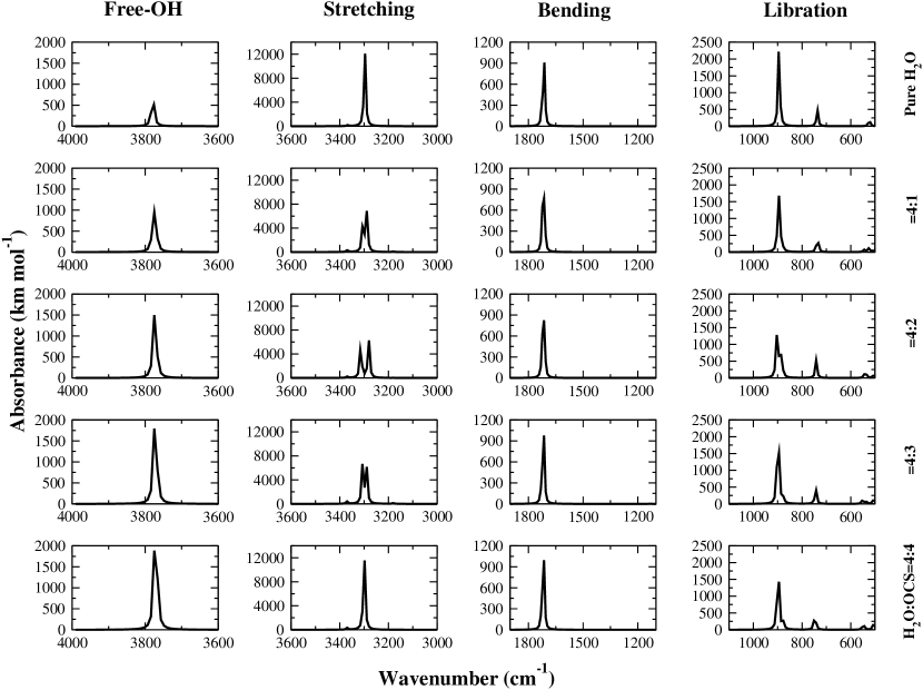
Figure A11: Absorption spectra of the four modes for water ice for the five measured compositions, ranging from pure water ice (top) to 4:4 H₂O-OCS mixture (bottom).

Garozzo et al. ⁹⁸ proposed that carbonyl sulfide (OCS) is a key ingredient of the grain surface. Its abundance in ice phase may vary between 0.05 and $0.15$% ¹⁶. Figure 1i shows the optimized structure of the 4:4 H₂O-OCS. Since oxygen is more electronegative than sulfur, the O atom of the OCS molecule is hydrogen-bonded to the water free-hydrogens. In the Appendix, Figure A11 shows the absorption IR band spectra for H₂O-OCS clusters with various concentrations. Figure 5h depicts the band strengths as a function of the concentration of OCS. Here, the free-OH mode is the most affected and its band strength increases with the concentration of OCS. All other modes roughly remain invariant by varying the amount of impurity.

4.2.4 N₂ ice

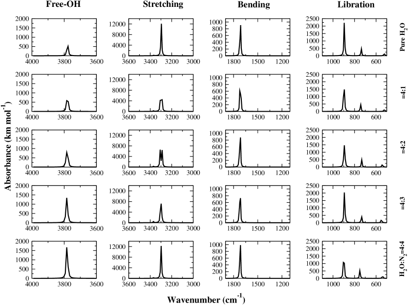
Figure A12: Absorption spectra of the four modes for water ice for the five measured compositions, ranging from pure water ice (top) to 4:4 H₂O-N₂ mixture (bottom).

N₂ is a stable homonuclear molecule and, due to its symmetry, it is infrared inactive. However, when embedded in an ice matrix, the crystal field breaks the symmetry, and an infrared transition is activated around $2325.58$ cm^-1 ($4.30$ $\mu$m). Figure 1j shows the optimized geometry of the H₂O-$\rm{N_{2}}$ system with a $4:4$ ratio. The IR absorption spectra of water ice containing different amounts of $\rm{N_{2}}$ are shown in the Appendix (see Figure A12). The corresponding peak frequencies and intensities are provided in the Appendix as well (see Table A2). The dependence of the band strengths on the N₂ concentration is depicted in Figure 5i. It has been found that the slope of the band strength of the libration mode decreases, whereas the bending, stretching, and free OH modes show an increasing trend with the concentration of N₂. The linear fitting coefficients are provided in Table 4. Figure 9c shows the comparison of band strengths with and without considering the dispersion effects. It is noted that the inclusion of dispersion effect leads to small changes.

4.2.5 O₂ ice

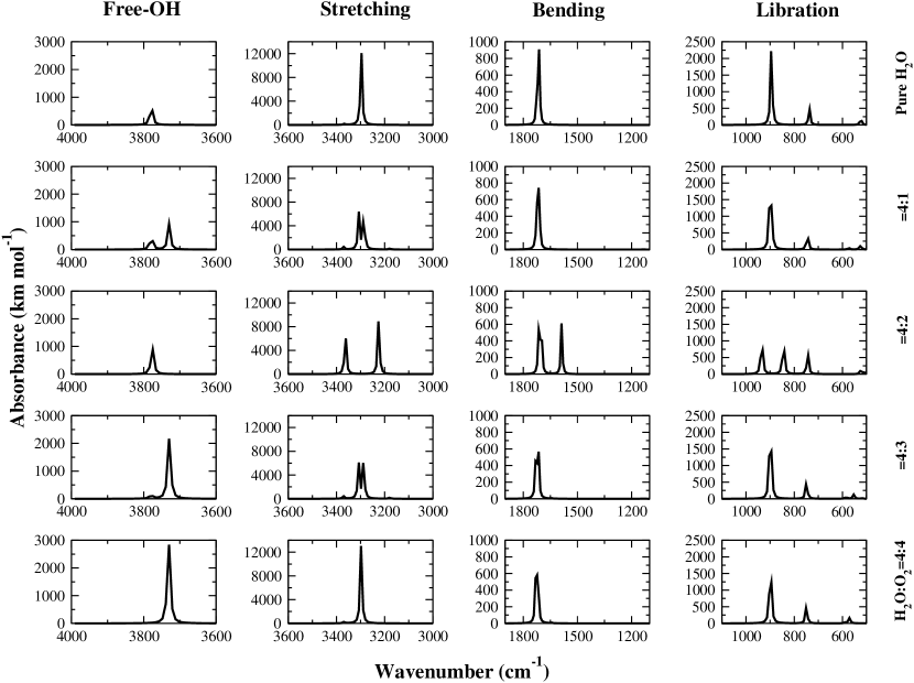
Figure A13: Absorption spectra of the four modes for water ice for the five measured compositions, ranging from pure water ice (top) to 4:4 H₂O-O₂ mixture (bottom).

Analogously to $\rm{N_{2}}$, $\rm{O_{2}}$ is a homonuclear molecule, which is infrared inactive except when it is embedded in an ice matrix ^{99, 100}, thus giving rise to an absorption band around $1550.39$ cm^-1 ($6.45$ $\mu$m). $\rm{O_{2}}$ ice is not much abundant because the largest part of the oxygen budget in the dense molecular clouds is locked in the form of $\rm{CO_{2}}$, CO, water ice, and silicates. The optimized geometry of the $4:4$ H₂O-$\rm{O_{2}}$ ratio is shown in Figure 1k. IR spectra for different concentrations (Figure A13) and the corresponding peak frequencies and intensities (Table A2) are provided in the Appendix. The dependence of band strengths upon O₂ concentration is shown in Figure 5j. Similarly to the $\rm{N_{2}}$-water case, the free-OH mode is the most affected. The slope of the band strength of the libration and bending modes decreases, whereas the stretching and free-OH modes show an increasing trend with the concentration of O₂. The fitting coefficients for different H₂O-N₂ mixtures are provided in Table 4.

Figure 9d depicts the comparison of the band strengths with and without the inclusion of dispersion effects for the H₂O-O₂ system. It is evident that trend of the band strength with the impurity concentration slightly increases for the libration mode, whereas slightly decreases for the stretching mode when corrections for dispersion effects are present. In the case of the bending mode, the band strength rapidly increases, whereas the band strength rapidly decreases for the free OH mode.

4.2.6 Comparison between various mixtures

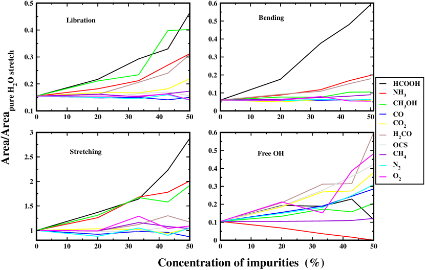
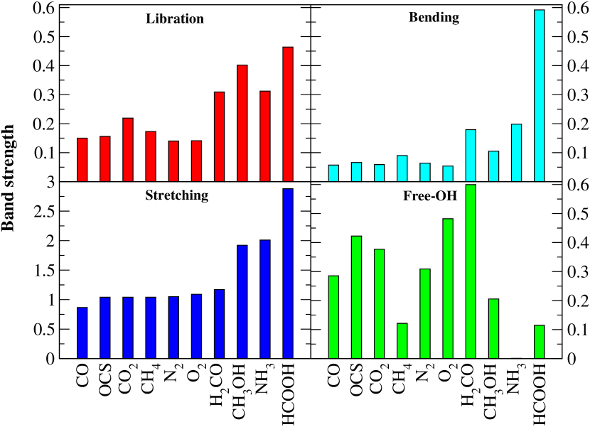
Figure 10: Top panel: Effect of impurities on the four fundamental vibrational modes of water. Bottom panel: Comparison of the band strengths for the four fundamental vibrational modes as affected by impurities.

To compare the effect of all impurities considered in this study on the band strength, we have plotted the band profiles of the four fundamental modes of water ice as a function of the concentration of impurities, the results being shown in Figure 10, top panel. For all fundamental modes, band strengths increase with the concentration of $\rm{CH_{3}OH}$, $\rm{H_{2}CO}$, HCOOH, $\rm{CH_{4}}$. To better understand their effect, in Figure 10, bottom panel, we report the relative band strengths for the $4:4$ ratio mixtures. From this, it is clear that the libration, bending, and stretching modes are mostly affected by formic acid, while the free-OH mode is mostly affected by formaldehyde. An interesting feature is found for the free-OH mode for the $\rm{NH_{3}-H_{2}O}$ system. By increasing the $\rm{NH_{3}}$ concentration with respect to pure water, the band strength of the free-OH mode decreases and disappears when the 4 : 4 concentration ratio is reached.

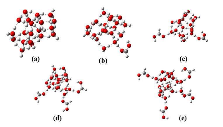
Figure S3: Structure of water clusters containing 20 $\rm{H_{2}O}$ molecules with HCOOH as impurity in different concentration ratio: (a) pure water, (b) $\rm{H_{2}O:HCOOH=20:1}$, (c) $\rm{H_{2}O:HCOOH=10:1}$, (d) $\rm{H_{2}O:HCOOH=6.67:1}$, (e) $\rm{H_{2}O:HCOOH=5:1}$.

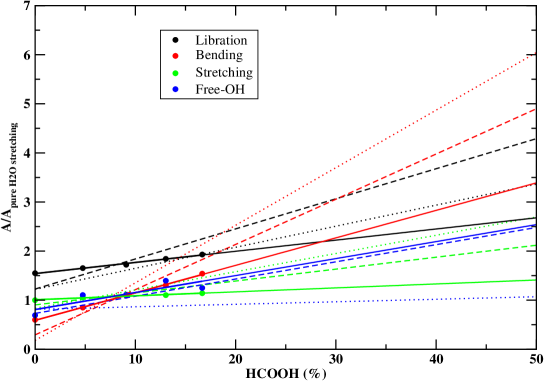
Figure S4: Comparison of the band strength of the four fundamental vibrational modes for water clusters containing 20$\rm{H_{2}O}$, 6H₂O, and 4H₂O molecules with HCOOH as an impurity in different concentrations. Solid lines represent the band strength profiles for 20H₂O cluster, dotted lines for the water c-hexamer (chair) (6H₂O), and dashed lines for water c-tetramer (4H₂O).

Figure S1 (in the SI) depicts the optimized structures of the pure water c-hexamer (chair) configuration along with those obtained for a 6:1 concentration ratio. Figure S2 (in the SI) collects the results for the band strength variations for the c-hexamer (chair) water cluster configuration is considered, this being analogous to Figure 5. The geometries of water clusters containing $20$ water molecules with HCOOH as an impurity in various concentrations are shown in Figure S3 (in the SI) and the corresponding variations of the band strengths with increasing concentration of HCOOH are depicted in Figure S4 (in the SI). This figure also reports the comparison of band strength profiles for different water clusters. The structures of the 20-water-molecule cluster have been taken from Shimonishi et al. ¹⁰¹, and were obtained by MD-annealing calculations using classical force-fields to reproduce a water cluster as a model of the ASW surface. The comparison shown in Figure S4 (in the SI) demonstrates that the 4H₂O model provides results similar to those obtained with 6 and 20 water molecules. This furthermore confirms the validity of our approach.

5 Conclusions

Water ice is known to be the major constituent of interstellar icy grain mantles. Interestingly, there have been several astronomical observations ^{102, 41} of the OH stretching and HOH bending modes at $3278.69$ cm^-1 ($3.05$ $\mu$m) and $1666.67$ cm^-1 ($6.00$ $\mu$m), respectively. It is noteworthy that the intensity ratio of these two bands is very different from what obtained in laboratory experiments for pure water ice. This suggested that the presence of impurities in water ice affects the spectroscopic features of water itself. For this reason, a series of laboratory experiments were carried out in order to explain the discrepancy between observations and experiments. Furthermore, these observations prompted us to perform an extensive computational investigation aiming to evaluate the effect of different amounts of representative impurities on the band strengths and absorption band profiles of interstellar ice. We selected the most abundant impurities ($\rm{HCOOH,\ NH_{3},\ CH_{3}OH,\ CO,\ CO_{2},\ H_{2}CO,\ CH_{4},\ OCS,\ N_{2}}$, and $\rm{O_{2}}$) and studied their effect on four fundamental vibrational bands of pure water ice by employing different cluster models. Indeed, both the experimental and theoretical peak positions might differ from the astronomical observations. This is because the grain shape, size, and constituents, the surrounding physical conditions, and the presence of impurities play a crucial role in tuning the ice spectroscopic features.

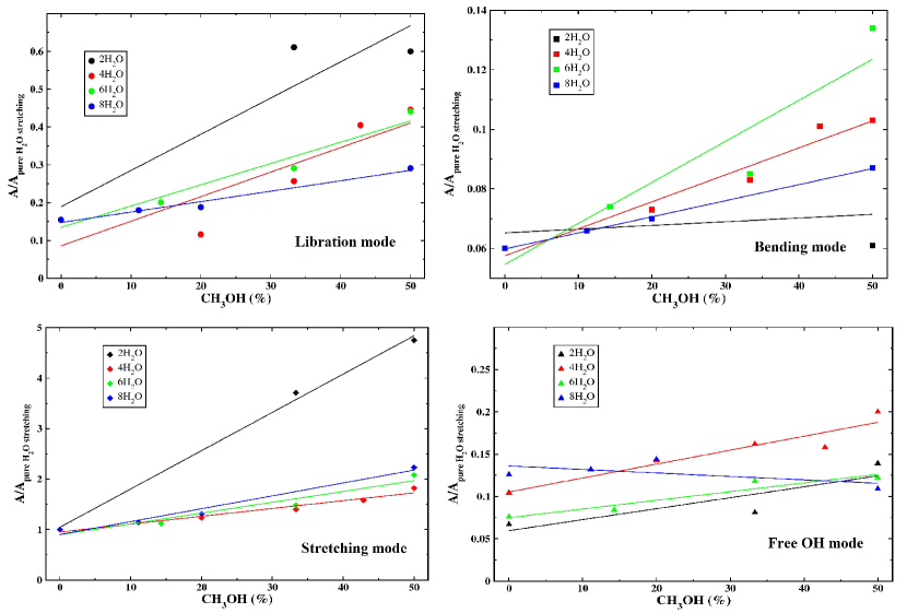
Figure S5: Effect of the cluster size on the band strength profile.

Although most of the computations were performed for a cluster containing only four water molecules as a model system (to find a trend in the absorption band strength), we demonstrated that increasing the size of the cluster would change the band strength profile only marginally. From the band strength profiles shown in Figure S5 (in the SI), it is apparent that the stretching mode is the most affected and the bending mode is the least affected by the presence of impurities. Libration, bending, and bulk stretching modes were found to be most affected by HCOOH impurity, followed by $\rm{CH_{3}OH}$ and $\rm{H_{2}CO}$. Another interesting point to be noted is that the band strength of the free-OH stretching mode decreases with increasing concentration of $\rm{NH_{3}}$ and completely vanishes when the concentration of NH₃ becomes 50%. Most interestingly, the experimental free-OH band profile shows a decreasing trend when water is mixed with $\rm{NH_{3}}$ (Figure 7, right panel), similarly to that obtained computationally.

Finally, our computed and laboratory absorption spectra of water-rich ices will be part of a larger infrared ice database in support of current and future observations. Understanding the effect of impurities in interstellar polar ice analogs will be pivotal to support the unambiguous identification of COMs in interstellar ice mantles by using future space missions such as JWST ⁹.

6 Acknowledgment

PG acknowledges the support of CSIR (Grant No. 09/904(0013) 2K18 EMR-I). MS gratefully acknowledges DST-INSPIRE Fellowship [IF160109] scheme. AD acknowledges ISRO respond (Grant No. ISRO/RES/2/402/16-17). This research was possible in part due to a Grant-In-Aid from the Higher Education Department of the Government of West Bengal. SI acknowledges the Royal Society for financial support. ZK was supported by VEGA – The Slovak Agency for Science, Grant No. 2/0023/18. This work was also supported by COST Action TD1308 – ORIGINS.

7 Supporting Information (SI)

Optimized structures of water clusters and impurities mixed with a 6:1 concentration ratio (Figure S1); band strengths of the four fundamental vibration modes of water clusters containing impurities with various concentrations (Figure S2); structure of water clusters containing 20 H₂O molecules with HCOOH as impurity in different concentration ratio (Figure S3); comparison of the band strength of various water clusters mixed with HCOOH (Figure S4); effect of the cluster size on the band strength profile (Figure S5); harmonic infrared frequencies and intensities of the 4H₂O cluster (Table S1), 4H₂O/HCOOH (Table S2), 4H₂O/2HCOOH (Table S3), 4H₂O/3HCOOH (Table S4), 4H₂O/4HCOOH (Table S5), 4H₂O/NH₃ (Table S6), 4H₂O/2NH₃ (Table S7), 4H₂O/3NH₃ (Table S8), 4H₂O/4NH₃ (Table S9) evaluated at the B2PLYP/maug-cc-pVTZ level; harmonic infrared frequencies and intensities of the H₂O^QM + 3 H₂O^MM complex (Table S10); harmonic infrared frequencies and intensities of the first 4 H₂O^QM+16 H₂O^MM: complex configuration 1 (Table S11) and complex configuration 2 (Table S12); geometric details of optimized structures of water clusters and impurities mixed with 4:4 and 6:1 concentration ratios (Optimized-Structures.zip). The Supporting Information is available free of charge on the ACS Publications website.

Appendix

Table A1: Comparison of band positions and band intensities as obtained by different quantum-chemical methods.

Assignment	4H2O+PCM,		4H2O+PCM,		1H2O(QM)+3H2O(MM)		4H2O(QM)+16H2O(MM)
	B3PLYP/6-31G(d)		B2PLYP/m-aug-cc-pVTZ		+PCM, B3PLYP/6-31G(d)		+PCM, B3PLYP/6-31G(d)
	Wavenumber	Intensity	Wavenumber	Intensity	Wavenumber	Intensity	Wavenumber	Intensity
	(cm-1)	(km/mol)	(cm-1)	(km/mol)	(cm-1)	(km/mol)	(cm-1)	(km/mol)
1							28.5053	1.6212
2							32.4112	0.3452
3			39.3404	0.0000	39.0097	3.5702	40.5682	1.9422
4	42.31	0.000					42.6937	0.9658
5							45.5125	2.8291
6							47.0457	2.4796
7							51.1545	1.5206
8							53.0040	0.4852
9							57.4113	4.9283
10							58.9090	1.5004
11							62.8440	3.3091
12							64.6577	0.5053
13							67.1132	0.4600
14					70.0478	0.9941	71.0670	1.0092
15							72.1009	5.5430
16							78.5377	1.2279
17							79.5809	2.8592
18			85.5169	4.1241			84.0856	0.3164
19							88.1866	0.5336
20							91.6244	1.1620
21	101.53	0.5953			107.4593	248.8304	95.9146	1.9115
22					114.669	81.5288	131.1634	139.0258
23					134.1712	121.9418	147.4509	6.2284
24							155.1556	1.5936
25							157.0881	12.4196
26							163.8254	4.8492
27							169.5773	3.8618
28							173.1802	11.6779
29							177.8697	22.1882
30							179.4412	3.0508
31							189.5523	12.2882
32							193.8849	18.7990
33							199.5633	30.2086
34			202.1393	0.0000			203.7815	44.7590
35							205.2272	29.8834
36							210.7469	42.9633
37							212.8473	18.5861
38							215.6034	104.3096
39							219.2947	9.1183
40			222.9069	104.7500			221.2358	136.0590
41			22.29069	104.7500			223.7398	14.6743
42							226.9991	92.7095
43							229.4667	11.8754
44			231.0105	94.8938			231.1955	180.5173
45							235.9253	6.3462
46	243.67	0.000	240.0832	0.6734			239.8566	146.4113
47			246.4688	287.8694	251.1220	19.7407	249.2394	2.9212
48			246.4688	287.8694	253.1088	18.8069	254.8166	52.0837
49							260.4354	12.2059
50	277.10	206.9799	274.1815	0.000	270.4875	7.7664	270.0093	13.8498
51	277.10	206.9799			286.0773	10.8931	280.9175	13.8528
52	281.08	0.3532					284.5581	1.3055
53							286.3104	31.7468
54	301.85	0.1654					307.5132	4.0551
55	307.74	298.2083					308.3710	4.8097
56	307.74	298.2083					314.4016	25.2868
57							319.3857	8.4817
58	327.52	0.0000			331.3394	156.5948	330.7679	1.3826
59							334.6995	4.4240
60							347.3954	4.9640
61			398.6011	0.000			387.1876	8.8358

Assignment	4H2O+PCM,		4H2O+PCM,		1H2O(QM)+3H2O(MM)		4H2O(QM)+16H2O(MM)
	B3PLYP/6-31G(d)		B2PLYP/m-aug-cc-pVTZ		+PCM, B3PLYP/6-31G(d)		+PCM, B3PLYP/6-31G(d)
	Wavenumber	Intensity	Wavenumber	Intensity	Wavenumber	Intensity	Wavenumber	Intensity
	(cm-1)	(km/mol)	(cm-1)	(km/mol)	(cm-1)	(km/mol)	(cm-1)	(km/mol)
62			427.5608	44.2017	417.2017	11.4416	426.8869	78.1914
63							432.7664	47.4011
64			443.1204	79.6160			449.0251	78.8810
65			443.1204	79.6160			455.8202	9.0749
66							458.4089	52.9014
67							461.3395	7.1542
68							468.0311	44.1926
69	473.37	0.000					476.0688	5.2943
70					483.9590	107.2607	483.8486	73.9300
71							500.1090	30.3953
72					502.7496t	211.3432	500.9839	36.5412
73							508.1366	20.0694
74							512.3840	13.9454
75	523.50	58.1147					532.3995	46.0624
76	523.76	0.9980			539.1224t	59.4593	535.4481	4.4789
77	523.76	0.9980					543.6866	60.5730
78							545.4049	57.7011
79							557.0745	41.0189
80							560.6706	18.2338
81							581.7986	25.4989
82							585.3805	214.1458
83							588.1325	72.1128
84t							593.3498	6.1937
85t							598.2759	204.0196
86t					620.5928t	2.9662	620.7530	378.5822
87t							623.3143	58.9759
88t							629.3486	219.1103
89t							639.6399	56.7824
90t							642.7590	240.6043
91t							648.3193	65.9335
92t							658.9772	36.8759
93t					670.5374t	209.1029	676.8776	176.4931
94t							679.7026	594.2500
95t			683.4168	312.1539			685.0436	47.0063
96t							690.6345	554.1850
97t							695.3495	353.6124
98t							699.7148	156.7689
99t							704.2320	32.3584
100t							721.7785	334.5258
101t	737.11t	144.3682			734.0061t	476.6369	725.6449	111.7286
102t							728.6757	454.3782
103t							747.1205	168.5362
104t							753.5614	192.6962
105t							765.5413	275.9737
106t			778.3957t	237.5051			766.1653	425.8765
107t			778.3957t	237.5051			772.0067	356.3800
108t							803.0436	327.2798
109t							818.6290	277.6746
110t							839.8062	313.0187
111t	894.95t	342.8199			870.1429t	201.9038	850.6360	671.1597
112t	894.95t	342.8199	934.3601t	0.000			929.4103	415.2180
113t							955.5738	180.7041
114t	1127.57t	0.000					966.2260	55.4464
115b							1401.1608	328.9992
116b							1404.9892	279.6521
117b					1407.2265b	191.4554	1406.8655	454.2350
118b							1412.4834	218.9410
119b							1415.0050	217.1485
120b							1416.7673	553.3807

Assignment	4H2O+PCM,		4H2O+PCM,		1H2O(QM)+3H2O(MM)		4H2O(QM)+16H2O(MM)
	B3PLYP/6-31G(d)		B2PLYP/m-aug-cc-pVTZ		+PCM, B3PLYP/6-31G(d)		+PCM, B3PLYP/6-31G(d)
	Wavenumber	Intensity	Wavenumber	Intensity	Wavenumber	Intensity	Wavenumber	Intensity
	(cm-1)	(km/mol)	(cm-1)	(km/mol)	(cm-1)	(km/mol)	(cm-1)	(km/mol)
121b					1422.8362b	445.8394	1423.8136	320.7421
122b							1427.0557	239.2493
123b							1431.3527	280.4839
124b							1433.6066	107.3301
125b							1436.1459	143.6834
126b							1442.3811	59.3969
127b					1456.6860b	64.4541	1456.0330	69.7821
128b							1465.8850	261.4679
129b							1481.4184	129.4706
130b							1490.6689	54.4350
131b	1711.28b	251.8157	1630.3695b	176.7723	1764.1323b	143.3391	1759.3916	113.0751
132b	1723.10b	82.9912	1647.3535b	74.0296			1781.9431	109.2325
133b	1723.10b	82.9911	1647.3536b	74.0296			1805.1440	185.2649
134b	1741.00b	0.0000	1672.6698b	0.000			1821.5031	81.3961
135s	3182.21s	0.0000					3277.1620	1061.3522
136s	3297.07s	1871.6907					3379.4017	1450.1515
137s	3297.07s	1871.6907	3411.5900s	0.000	3399.8219s	161.5281	3415.3773	260.6407
138s	3366.39s	50.2255	3477.3996s	1793.2478			3441.1055	54.0971
139s			3477.3996s	1793.2478			3501.0930	137.3189
140s							3510.2084	280.1448
141s							3515.4119	164.7163
142s			3522.3300s	2.0149			3527.1563	98.4213
143s					3533.5836s	119.6470	3532.0223	374.1860
144s							3535.9755	331.7897
145s							3539.5696	667.4359
146s							3541.9090	42.2047
147s							3546.9082	185.0747
148s							3549.9374	209.7596
149s							3555.5498	189.4891
150s							3558.8959	76.1871
151s					3561.1437s	374.8984	3563.2840	189.8014
152s							3568.4433	217.3753
153s							3575.4761	97.1563
154s							3576.5391	86.9267
155s					3579.9423s	110.7922	3579.7822	19.6952
156s							3589.8658	38.6004
157s							3590.2134	57.5165
158s							3603.0421	149.2000
159s							3618.1897	266.3486
160s							3620.8200	224.9253
161s							3622.0658	233.3283
162s							3623.0520	397.9328
163s							3624.0959	35.3011
164s							3626.6346	276.1415
165s							3630.3037	955.2942
166s							3631.8424	16.4537
167s							3633.8572	248.7481
168f					3643.1130f	84.3280	3646.1348	108.4691
169f					3647.6874f	450.2363	3650.9996	175.2420
170f					3651.3875f	90.6885	3652.3329	128.0414
171f	3778.38f	126.4545	3864.6871f	144.7620			3652.8838	205.0487
172f	3779.79f	52.8022	3865.9912f	138.6232			3653.3844	33.2033
173f	3779.79f	52.8022	3865.9912f	138.6232			3653.8800	205.2072
174f	3781.36f	0.0000	3867.1847f	0.0000	3797.0095f	37.5965	3654.0193	86.2440

Notes: ^tOH torsion; ^bOH scissoring; ^sOH stretching; ^ffree OH. For the conversion of km/mol to cm molecule^-1, intensity values need to multiply by a factor $\rm{1.6603\times 10^{-19}}$.

Table A2: Frequencies, integral absorbance coefficients, and normal modes of vibration of H₂O-X (X = HCOOH, $\rm{NH_{3}}$, $\rm{CH_{3}OH}$, CO, $\rm{CO_{2}}$, $\rm{H_{2}CO}$, $\rm{CH_{4}}$, OCS, $\rm{N_{2}}$, and $\rm{O_{2}}$)

$\rm{H_{2}O:X}$	Frequency at peak	Integral absorbance	Modes of
	in cm-1 ($\mu$m)	coefficient in	vibration
		cm molecule-1
HCOOH
1:0.25	875.47 (11.42)	$5.98\times 10^{-17}$	OH torsion
	1698.42 (5.89)	$5.24\times 10^{-17}$	H2O scissoring
	3326.84 (3.00)	$1.88\times 10^{-16}$	OH stretching
	3635.02 (2.75)	$4.11\times 10^{-17}$	free OH
1:0.50	859.72 (11.63)	$6.18\times 10^{-17}$	OH torsion
	1696.3 (5.90)	$5.37\times 10^{-17}$	H2O scissoring
	3341.67 (2.99)	$2.08\times 10^{-16}$	OH stretching
	3632.99 (2.75)	$4.19\times 10^{-17}$	free OH
1:0.75	878.28 (11.38)	$4.91\times 10^{-17}$	OH torsion
	1688.62 (5.92)	$6.27\times 10^{-17}$	H2O scissoring
	3260.11 (3.07)	$2.46\times 10^{-16}$	OH stretching
	3611.81 (2.77)	$6.46\times 10^{-17}$	free OH
1:1.00	747.49 (13.38)	$9.21\times 10^{-17}$	OH torsion
	1685.24 (5.93)	$7.56\times 10^{-17}$	H2O scissoring
	3343.53 (2.99)	$2.08\times 10^{-16}$	OH stretching
	3608.22 (2.77)	$7.15\times 10^{-17}$	free OH
NH3
1:0.25	886.69 (11.28)	$7.31\times 10^{-17}$	OH torsion
	1717.36 (5.82)	$3.58\times 10^{-17}$	H2O scissoring
	3055.07 (3.27)	$2.20\times 10^{-16}$	OH stretching
	3778.71 (2.65)	$1.16\times 10^{-17}$	free OH
1:0.50	877.63 (11.39)	$8.92\times 10^{-17}$	OH torsion
	1725.39 (5.80)	$3.28\times 10^{-17}$	H2O scissoring
	3127.37 (3.20)	$4.38\times 10^{-16}$	OH stretching
	3737.41 (2.65)	$7.02\times 10^{-18}$	free OH
1:0.75	859.21 (11.64)	$4.99\times 10^{-17}$	OH torsion
	1730.52 (5.78)	$2.47\times 10^{-17}$	H2O scissoring
	3264.44 (3.06)	$4.27\times 10^{-16}$	OH stretching
	3777.53 (2.65)	$5.89\times 10^{-18}$	free OH
1:1.00	938.38 (10.66)	$9.35\times 10^{-17}$	OH torsion
	1751.53 (5.71)	$4.43\times 10^{-17}$	H2O scissoring
	3270.01 (3.06)	$4.90\times 10^{-16}$	OH stretching
	–	–	free OH
CH3OH
1:0.25	751.68 (13.30)	$5.60\times 10^{-17}$	OH torsion
	1703.98 (5.87)	$3.85\times 10^{-17}$	H2O scissoring
	3252.5 (3.07)	$2.33\times 10^{-16}$	OH stretching
	3774.67 (2.65)	$1.73\times 10^{-17}$	free OH
1:0.50	719.11 (13.91)	$7.67\times 10^{-17}$	OH torsion
	1654.59 (6.04)	$3.62\times 10^{-17}$	H2O scissoring
	3207.15 (3.12)	$4.57\times 10^{-16}$	OH stretching
	3843.18 (2.60)	$2.26\times 10^{-17}$	free OH
1:0.75	702.71 (14.23)	$5.49\times 10^{-17}$	OH torsion
	1690.03 (5.92)	$2.92\times 10^{-17}$	H2O scissoring
	3351.12 (2.96)	$2.25\times 10^{-16}$	OH stretching
	3783.4 (2.64)	$1.72\times 10^{-17}$	free OH
1:1.00	906.29 (11.03)	$6.61\times 10^{-17}$	OH torsion
	1693.39 (5.90)	$2.96\times 10^{-17}$	H2O scissoring
	3295.67 (3.03)	$3.97\times 10^{-16}$	OH stretching
	3774.54 (2.65)	$2.03\times 10^{-17}$	free OH

$\rm{H_{2}O:X}$	Frequency at peak	Integral absorbance	Modes of
	in cm-1 ($\mu$m)	coefficient in	vibration
		cm molecule-1
CO
1:0.25	895.46 (11.17)	$5.70\times 10^{-17}$	OH torsion
	1711.46 (5.84)	$4.14\times 10^{-17}$	H2O scissoring
	3290.66 (3.04)	$3.14\times 10^{-16}$	OH stretching
	3791.25 (2.64)	$2.39\times 10^{-17}$	free OH
1:0.50	898.71 (11.13)	$5.64\times 10^{-17}$	OH torsion
	1711.73 (5.84)	$4.19\times 10^{-17}$	H2O scissoring
	3285.68 (3.04)	$3.22\times 10^{-16}$	OH stretching
	3791.07 (2.64)	$2.42\times 10^{-17}$	free OH
1:0.75	898.22 (11.13)	$5.71\times 10^{-17}$	OH torsion
	1713.47 (5.84)	$4.18\times 10^{-17}$	H2O scissoring
	3290.55 (3.04)	$3.16\times 10^{-16}$	OH stretching
	3789.19 (2.64)	$4.93\times 10^{-17}$	free OH
1:1.00	899.44 (11.12)	$5.89\times 10^{-17}$	OH torsion
	1715.94 (5.83)	$4.22\times 10^{-17}$	H2O scissoring
	3293.09 (3.04)	$3.13\times 10^{-16}$	OH stretching
	3789.31 (2.64)	$6.92\times 10^{-17}$	free OH
CO2
1:0.25	893.79 (11.19)	$5.63\times 10^{-17}$	OH torsion
	1710.62 (5.84)	$4.23\times 10^{-17}$	H2O scissoring
	3288.08 (3.04)	$3.10\times 10^{-16}$	OH stretching
	3766.88 (2.65)	$3.85\times 10^{-17}$	free OH
1:0.50	890.45 (11.23)	$5.72\times 10^{-17}$	OH torsion
	1713.11 (5.84)	$4.22\times 10^{-17}$	H2O scissoring
	3278.84 (3.05)	$3.26\times 10^{-16}$	OH stretching
	3767.04 (2.65)	$4.21\times 10^{-17}$	free OH
1:0.75	891.90 (11.21)	$5.98\times 10^{-17}$	OH torsion
	1709.11 (5.85)	$4.20\times 10^{-17}$	H2O scissoring
	3294.04 (3.04)	$3.17\times 10^{-16}$	OH stretching
	3766.76 (2.65)	$5.31\times 10^{-17}$	free OH
1:1.00	896.53 (11.15)	$5.61\times 10^{-17}$	OH torsion
	1709.45 (5.85)	$4.41\times 10^{-17}$	H2O scissoring
	3296.79 (3.03)	$3.05\times 10^{-16}$	OH stretching
	3765.50 (2.66)	$7.28\times 10^{-17}$	free OH
H2CO
1:0.25	890.85 (11.22)	$6.00\times 10^{-17}$	OH torsion
	1712.86 (5.84)	$3.97\times 10^{-17}$	H2O scissoring
	3274.97 (3.05)	$3.06\times 10^{-16}$	OH stretching
	3607.83 (2.77)	$8.46\times 10^{-17}$	free OH
1:0.50	886.56 (11.28)	$5.44\times 10^{-17}$	OH torsion
	1710.12 (5.85)	$4.17\times 10^{-17}$	H2O scissoring
	3246.10 (3.08)	$3.27\times 10^{-16}$	OH stretching
	3601.67 (2.78)	$9.12\times 10^{-17}$	free OH
1:0.75	937.07 (10.67)	$5.41\times 10^{-17}$	OH torsion
	1767.86 (5.66)	$2.81\times 10^{-17}$	H2O scissoring
	3279.19 (3.05)	$3.23\times 10^{-16}$	OH stretching
	3607.45 (2.77)	$1.35\times 10^{-17}$	free OH
1:1.00	904.32 (11.06)	$5.51\times 10^{-17}$	OH torsion
	1713.74 (5.84)	$3.51\times 10^{-17}$	H2O scissoring
	3338.99 (2.99)	$2.96\times 10^{-16}$	OH stretching
	3612.36 (2.77)	$9.67\times 10^{-17}$	free OH

$\rm{H_{2}O:X}$	Frequency at peak	Integral absorbance	Modes of
	in cm-1 ($\mu$m)	coefficient in	vibration
		cm molecule-1
CH4
1:0.25	903.11 (11.07)	$5.96\times 10^{-17}$	OH torsion
	1710.29 (5.85)	$4.14\times 10^{-17}$	H2O scissoring
	3287.91 (3.04)	$3.06\times 10^{-16}$	OH stretching
	3777.98 (2.65)	$2.03\times 10^{-17}$	free OH
1:0.50	910.32 (10.98)	$5.97\times 10^{-17}$	OH torsion
	1706.49 (5.86)	$4.14\times 10^{-17}$	H2O scissoring
	3280.67 (3.05)	$3.30\times 10^{-16}$	OH stretching
	3778.16 (2.65)	$2.16\times 10^{-17}$	free OH
1:0.75	905.03 (11.05)	$6.05\times 10^{-17}$	OH torsion
	1706.58 (5.86)	$4.10\times 10^{-17}$	H2O scissoring
	3296.35 (3.03)	$3.22\times 10^{-16}$	OH stretching
	3778.86 (2.65)	$2.18\times 10^{-17}$	free OH
1:1.00	893.41 (11.19)	$6.23\times 10^{-17}$	OH torsion
	1705.91 (5.86)	$4.11\times 10^{-17}$	H2O scissoring
	3312.78 (3.02)	$3.41\times 10^{-16}$	OH stretching
	3777.04 (2.65)	$2.40\times 10^{-17}$	free OH
OCS
1:0.25	897.72 (11.14)	$5.74\times 10^{-17}$	OH torsion
	1711.96 (5.84)	$4.11\times 10^{-17}$	H2O scissoring
	3288.8 (3.04)	$3.10\times 10^{-16}$	OH stretching
	3772.38 (2.65)	$4.82\times 10^{-17}$	free OH
1:0.50	889.91 (11.24)	$5.80\times 10^{-17}$	OH torsion
	1712.15 (5.84)	$4.30\times 10^{-17}$	H2O scissoring
	3281.28 (3.05)	$3.27\times 10^{-16}$	OH stretching
	3772.57 (2.65)	$6.60\times 10^{-17}$	free OH
1:0.75	901.72 (11.09)	$5.77\times 10^{-17}$	OH torsion
	1713.88 (5.83)	$4.40\times 10^{-17}$	H2O scissoring
	3290.61 (3.04)	$3.26\times 10^{-16}$	OH stretching
	3771.53 (2.65)	$9.02\times 10^{-17}$	free OH
1:1.00	897.75 (11.14)	$5.75\times 10^{-17}$	OH torsion
	1713.97 (5.83)	$4.47\times 10^{-17}$	H2O scissoring
	3299.75 (3.03)	$3.29\times 10^{-16}$	OH stretching
	3770.63 (2.65)	$1.11\times 10^{-16}$	free OH
N2
1:0.25	894.31 (11.18)	$5.63\times 10^{-17}$	OH torsion
	1709.81 (5.85)	$4.16\times 10^{-17}$	H2O scissoring
	3292.23 (3.04)	$3.16\times 10^{-16}$	OH stretching
	3778.08 (2.65)	$2.34\times 10^{-17}$	free OH
1:0.50	889.34 (11.24)	$5.98\times 10^{-17}$	OH torsion
	1716.33 (5.83)	$4.54\times 10^{-17}$	H2O scissoring
	3290.41 (3.04)	$3.10\times 10^{-16}$	OH stretching
	3778.76 (2.65)	$2.36\times 10^{-17}$	free OH
1:0.75	892.07 (11.21)	$5.98\times 10^{-17}$	OH torsion
	1716.67 (5.82)	$4.69\times 10^{-17}$	H2O scissoring
	3295.86 (3.03)	$3.05\times 10^{-16}$	OH stretching
	3784.28 (2.64)	$5.14\times 10^{-17}$	free OH
1:1.00	899.90 (11.11)	$5.73\times 10^{-17}$	OH torsion
	1714.47 (5.83)	$4.52\times 10^{-17}$	H2O scissoring
	3297.32 (3.03)	$3.15\times 10^{-16}$	OH stretching
	3780.99 (2.64)	$7.59\times 10^{-17}$	free OH

$\rm{H_{2}O:X}$	Frequency at peak	Integral absorbance	Modes of
	in cm-1 ($\mu$m)	coefficient in	vibration
		cm molecule-1
O2
1:0.25	893.78 (11.19)	$5.65\times 10^{-17}$	OH torsion
	1711.86 (5.84)	$4.11\times 10^{-17}$	H2O scissoring
	3286.24 (3.04)	$3.10\times 10^{-16}$	OH stretching
	3729.93 (2.68)	$4.41\times 10^{-17}$	free OH
1:0.50	934.71 (10.70)	$6.49\times 10^{-17}$	OH torsion
	1700.17 (5.88)	$3.78\times 10^{-17}$	H2O scissoring
	3225.04 (3.10)	$4.51\times 10^{-16}$	OH stretching
	3774.84 (2.65)	$2.77\times 10^{-17}$	free OH
1:0.75	892.96 (11.20)	$5.75\times 10^{-17}$	OH torsion
	1717.35 (5.82)	$4.04\times 10^{-17}$	H2O scissoring
	3286.59 (3.04)	$3.12\times 10^{-16}$	OH stretching
	3729.19 (2.68)	$8.72\times 10^{-17}$	free OH
1:1.00	900.52 (11.10)	$5.67\times 10^{-17}$	OH torsion
	1718.90 (5.82)	$4.18\times 10^{-17}$	H2O scissoring
	3299.52 (3.03)	$3.19\times 10^{-16}$	OH stretching
	3727.75 (2.68)	$1.08\times 10^{-16}$	free OH

Table S1: Harmonic infrared frequencies and intensities of the complex 4H₂O evaluated at the B2PLYP/maug-cc-pVTZ level.

NM	$\omega$ [cm-1]	IR Int. [Km/mole]
1	39.3404	0.0000
2	85.5169	4.1241
3	202.1393	0.0000
4	222.9069	104.7500
5	222.9069	104.7500
6	231.0105	94.8938
7	240.0832	0.6734
8	246.4688	287.8694
9	246.4688	287.8694
10	274.1815	0.0000
11	398.6011	0.0000
12	427.5608	44.2017
13	443.1204	79.6160
14	443.1204	79.6160
15	683.4168	312.1539
16t	778.3957	237.5051
17t	778.3957	237.5051
18t	934.3601	0.0000
19b	1630.3695	176.7723
20b	1647.3535	74.0296
21b	1647.3536	74.0296
22b	1672.6698	0.0000
23s	3411.5900	0.0000
24s	3477.3996	1793.2478
25s	3477.3996	1793.2478
26s	3522.3300	2.0149
27f	3864.6871	144.7620
28f	3865.9912	138.6232
29f	3865.9912	138.6232
30f	3867.1847	0.0000

Notes. ^tOH torsion; ^bOH scissoring; ^sOH stretching; ^ffree OH.

Table S2: Harmonic infrared frequencies and intensities of the complex 4H₂O/HCOOH evaluated at the B2PLYP/maug-cc-pVTZ level.

NM	$\omega$ [cm-1]	IR Int. [Km/mole]
1	7.4652	2.8797
2	21.6554	0.4836
3	31.8296	0.8007
4	45.1056	0.3993
5	61.0883	3.2003
6	99.9662	7.7802
7	176.7899	26.3202
8	190.2330	26.8829
9	212.6031	80.9785
10	214.8008	65.5508
11	229.1782	167.5034
12	238.5224	82.0767
13	255.2508	249.2937
14	283.6779	26.8213
15	291.4533	55.7068
16	356.4031	83.8068
17	417.6885	49.4695
18	428.1868	57.7373
19	460.8606	57.1370
20	508.1693	55.1486
21	660.2176	284.6155
22	690.3556	83.8851
23t	754.6078	231.9718
24t	824.4685	178.7024
25t∗	939.4045	72.3782
26t∗	992.4637	143.3107
27	1085.0300	25.7493
28	1202.3494	398.5316
29	1404.3401	4.1326
30	1450.6121	11.3947
31b	1630.0596	190.6522
32b	1643.5475	74.8871
33b	1650.3969	67.4629
34b	1671.1011	2.8373
35	1727.4428	643.7374
36	3082.2813	261.4632
37s∗	3180.6017	2093.2108
38s∗	3305.3198	591.1162
39s	3439.5143	1097.5194
40s	3501.1192	960.3923
41s	3594.2178	538.8467
42f	3844.3939	126.6809
43f	3864.5499	125.4762
44f	3865.8634	156.4890
45f	3866.9802	55.7713

Notes. ^tOH torsion; ^bOH scissoring; ^sOH stretching; ^ffree OH; *vibrations contaminated by HCOOH modes.

Table S3: Harmonic infrared frequencies and intensities of the complex 4H₂O/2HCOOH evaluated at the B2PLYP/maug-cc-pVTZ level.

NM	$\omega$ [cm-1]	IR Int. [Km/mole]
1	4.6054	0.4281
2	13.0063	2.9178
3	16.5189	0.8051
4	19.0314	2.3774
5	20.9593	2.6393
6	33.4976	0.4467
7	36.7713	1.8500
8	42.5055	1.8790
9	57.0477	3.6453
10	87.6438	1.4306
11	98.3938	9.9521
12	109.3757	0.0813
13	179.0412	24.1400
14	190.5090	28.2740
15	214.0975	84.9229
16	218.8524	55.4812
17	230.2931	171.1476
18	238.6575	89.3090
19	267.3732	231.1914
20	283.3954	21.6224
21	299.6074	70.4602
22	358.3291	97.5174
23	418.1841	53.6749
24	433.0143	50.5761
25	453.3466	44.2133
26	511.7339	57.2963
27	626.1257	81.2731
28	663.5082	202.0801
29	664.5570	266.9661
30	690.0285	82.0272
31t	746.7845	238.4794
32t	832.5630	181.3816
33t∗	936.5175	69.8256
34t∗	992.1307	142.3809
35	1086.4569	25.8243
36	1100.7355	4.5531
37	1117.2066	421.1594
38	1202.1232	398.7897
39	1301.5992	19.3272
40	1403.7379	3.7351
41	1441.6206	5.0048
42	1449.0432	11.3813
43b	1630.1114	189.4041
44b	1643.0592	75.7767
45b	1650.4443	71.8600
46b	1671.6065	3.7550
47	1727.3571	640.6790
48	1740.9364	573.8795
49	3082.1544	256.8737
50s∗	3108.5982	9.0680
51s∗	3182.8047	2058.2321
52s∗	3311.8175	593.5776
53s	3443.5223	1123.8585
54s	3495.5861	975.1779
55s	3593.0205	538.1736
56	3722.9218	111.6916
57f	3843.8168	126.4406
58f	3860.4740	132.4083
59f	3863.8070	104.3051
60f	3865.7512	106.7733

Notes. ^tOH torsion; ^bOH scissoring; ^sOH stretching; ^ffree OH; *vibrations contaminated by HCOOH modes.

Table S4: Harmonic infrared frequencies and intensities of the complex 4H₂O/3HCOOH evaluated at the B2PLYP/maug-cc-pVTZ level.

NM	$\omega$ [cm-1]	IR Int. [Km/mole]
1	4.8748	0.5689
2	8.5054	0.7327
3	10.9091	1.7844
4	14.1204	2.2282
5	16.8372	1.6310
6	19.1432	3.8603
7	22.9673	0.5549
8	28.0702	2.8070
9	34.3674	0.6429
10	40.7401	1.8661
11	45.9916	0.3401
12	54.8514	5.3280
13	66.6228	5.5016
14	89.0988	1.1463
15	99.3575	2.6618
16	110.9935	9.9385
17	174.0921	44.5063
18	177.9118	30.6049
19	188.6541	24.0948
20	209.4056	83.4103
21	212.1508	55.0788
22	234.2838	28.4231
23	245.2791	210.0525
24	261.2989	35.4759
25	284.3732	27.8615
26	314.1459	145.9808
27	352.7412	77.0879
28	410.7784	41.6288
29	418.4381	142.3769
30	451.8321	62.9268
31	486.2526	26.6238
32	515.8604	43.5007
33	626.3452	78.8764
34	658.3748	265.4010
35	664.0178	196.3924
36	686.9044	88.1977
37	687.6686	73.9457
38t∗	798.2680	156.7957
39t	803.7700	211.1567
40t∗	926.7114	95.5456
41	949.5463	177.0601
42	1005.8276	134.0566
43	1083.1613	20.4516
44	1083.9241	23.7748
45	1098.4056	4.7221
46	1118.0234	421.3278
47	1198.2543	380.9330
48	1198.3514	418.6655
49	1303.1561	18.8667
50	1400.6093	4.0266
51	1400.7389	2.9534
52	1440.0730	5.2611
53	1445.8193	12.3688
54	1445.9512	8.9357
55b	1630.5379	192.0093
56b	1645.2809	74.7331
57b	1649.3090	90.0689
58b	1670.3929	1.3964
59	1729.0788	813.5933
60	1729.3363	445.0961

NM	$\omega$ [cm-1]	IR Int. [Km/mole]
61	1741.9079	575.8421
62	3085.0941	261.1337
63	3085.5154	98.0625
64	3110.4187	7.6777
65s∗	3215.3096	2288.1686
66s∗	3232.6395	1833.2038
67s∗	3306.6741	311.8714
68s	3451.6305	978.9670
69s	3473.6093	894.3564
70s	3609.3777	516.6451
71	3723.4615	111.6932
72f	3838.2715	172.2543
73f	3841.3048	97.0635
74f	3857.9521	119.5655
75f	3865.5487	121.3331

Notes. ^tOH torsion; ^bOH scissoring; ^sOH stretching; ^ffree OH; *vibrations contaminated by HCOOH modes.

Table S5: Harmonic infrared frequencies and intensities of the complex 4H₂O/4HCOOH evaluated at the B2PLYP/maug-cc-pVTZ level.

NM	$\omega$ [cm-1]	IR Int. [Km/mole]
1	5.2521	0.5902
2	6.6193	1.2706
3	8.8369	0.8598
4	9.6756	1.0009
5	14.2363	3.0419
6	15.7986	1.1225
7	18.3559	3.0357
8	19.2707	2.7650
9	22.1555	0.9922
10	27.4779	3.1848
11	30.7377	0.4104
12	36.6940	0.3940
13	42.5989	1.4605
14	50.4443	2.9039
15	56.1885	2.0333
16	67.8597	3.6648
17	79.8514	11.6336
18	88.6848	0.8582
19	101.4052	1.0586
20	120.4063	2.7295
21	173.0431	53.0876
22	174.6165	79.9014
23	181.6174	16.9912
24	193.2247	8.7228
25	207.4059	98.2327
26	209.4436	56.3457
27	214.9922	15.9518
28	251.9141	48.3664
29	260.0519	27.0848
30	277.2414	21.6313
31	294.7764	138.3103
32	370.6813	53.2423
33	411.5523	157.3717
34	426.8010	160.0370
35	432.4841	46.3694
36	474.7455	4.1043
37	500.7327	25.1590
38	506.2341	58.6370
39	626.8822	79.1196
40	662.8116	197.7640

NM	$\omega$ [cm-1]	IR Int. [Km/mole]
41t∗	680.2702	165.0245
42t∗	685.5338	74.2193
43t∗	685.8711	129.0114
44t	703.1086	134.5453
45t	777.4948	157.2018
46t∗	836.4350	145.9547
47	918.5370	51.5171
48	934.3780	130.8642
49	940.6167	399.9756
50	1005.3540	55.4131
51	1082.2723	15.9752
52	1082.8090	29.1817
53	1083.2383	8.1740
54	1096.9310	4.7996
55	1118.5677	421.7245
56	1194.7613	402.1943
57	1196.6655	678.8383
58	1196.9390	124.3700
59	1303.5269	19.2431
60	1398.1664	2.8858
61	1399.8325	2.3693
62	1400.1243	3.6218
63	1438.1358	3.4116
64	1443.1291	10.6650
65	1444.6815	8.9685
66	1445.0393	12.6099
67b	1633.0557	204.1450
68b	1645.9171	94.0994
69b	1651.0001	68.5795
70b	1672.8271	2.1359
71	1729.8409	773.0317
72	1729.9568	580.0062
73	1730.9646	527.5802
74	1742.3118	572.3800
75	3086.2791	171.0952
76	3087.0204	182.6391
77	3087.9488	105.7546
78	3114.3577	6.5557
79s∗	3235.8092	2226.0999
80	3251.6769	2145.0628
81s∗	3269.8018	1271.6200
82s∗	3338.7804	329.7573
83s	3451.7939	830.3998
84s	3506.2315	849.9293
85s	3580.2425	496.8387
86	3723.2687	112.7727
87f	3837.0764	199.2805
88f	3839.9016	135.3088
89f	3841.2858	85.4332
90f	3859.2614	129.2712

Notes. ^tOH torsion; ^bOH scissoring; ^sOH stretching; ^ffree OH; *vibrations contaminated by HCOOH modes.

Table S6: Harmonic infrared frequencies and intensities of the complex 4H₂O/NH₃ evaluated at the B2PLYP/maug-cc-pVTZ level.

NM	$\omega$ [cm-1]	IR Int. [Km/mole]
1	17.4723	1.6404
2	24.2573	2.7053
3	42.9718	9.2433
4	56.2828	14.2890
5	77.4675	5.3857
6	176.7386	14.5514
7	205.9991	61.5386
8	210.2974	51.1840
9	220.3754	138.5385
10	234.6966	41.4586
11	240.2432	175.3537
12	253.5984	22.5694
13	262.9908	199.8180
14	269.0541	36.5738
15	288.0112	25.8883
16	411.0477	10.8123
17	438.1929	57.2835
18	462.1627	115.4840
19	649.2280	90.3859
20t	673.7378	245.4033
21t	761.0067	286.3846
22t	785.5912	213.8984
23t	855.6009	110.1452
24	973.8257	54.6453
25	1133.1043	207.9712
26b	1635.5747	161.1828
27b	1648.9602	81.2871
28b∗	1654.1532	68.4123
29	1659.8070	23.9527
30b∗	1664.0270	13.9746
31b∗	1687.1189	4.9894
32s	3278.5997	1998.0299
33s	3358.0759	412.2786
34s	3442.1676	1170.0672
35	3483.9230	0.6553
36s	3499.4250	959.9493
37s	3600.3604	714.2057
38	3600.7264	13.1052
39	3601.5192	18.8438
40f	3865.2764	131.5539
41f	3866.4890	96.2050
42f	3867.7812	62.0566

Notes. ^tOH torsion; ^bOH scissoring; ^sOH stretching; ^ffree OH; *vibrations contaminated by NH₃ modes.

Table S7: Harmonic infrared frequencies and intensities of the complex 4H₂O/2NH₃ evaluated at the B2PLYP/maug-cc-pVTZ level.

NM	$\omega$ [cm-1]	IR Int. [Km/mole]
1	13.2137	3.5154
2	35.8031	4.5193
3	37.7152	15.3999
4	42.6399	0.6394
5	44.0908	1.0833
6	50.2282	25.2398
7	62.5104	1.7351
8	74.8511	7.5826
9	174.7854	0.3931
10	184.1028	49.5918
11	202.3520	59.3483
12	215.2501	3.8987
13	233.8400	170.4567
14	236.8583	13.8898
15	250.5424	28.2234
16	252.5110	43.5646
17	263.8678	24.6139
18	264.6765	198.4026
19	280.7045	30.8723
20	288.8026	34.1641
21	434.2362	2.5448
22	465.8322	178.0575
23	636.4757	5.8561
24	665.1100	92.9446
25t	688.2585	220.0675
26t	740.4480	369.3099
27t	786.8028	188.6747
28t	823.9109	101.1914
29t	894.7322	182.6960
30t	973.9338	41.1551
31	1131.1976	200.1314
32	1131.3535	216.3485
33b	1643.5894	150.8608
34b	1651.7575	100.8326
35b∗	1656.3567	54.5510
36b∗	1659.4699	6.3334
37	1660.0271	21.6415
38	1660.6689	23.4365
39b∗	1680.0902	25.5517
40b∗	1690.1602	1.1013
41s	3300.1629	879.2415
42s	3307.6453	2808.4413
43s	3377.2024	646.7542
44s	3391.5768	729.5638
45	3483.7965	0.9990
46	3483.9555	1.0499
47s	3578.8775	1603.7262
48s	3582.2181	63.0838
49	3600.8734	18.3990
50	3600.9540	18.6472
51	3601.2568	18.6290
52	3601.5982	18.6555
53f	3866.9165	77.0140
54f	3867.0372	90.8323

Notes. ^tOH torsion; ^bOH scissoring; ^sOH stretching; ^ffree OH; *vibrations contaminated by NH₃ modes.

Table S8: Harmonic infrared frequencies and intensities of the complex 4H₂O/3NH₃ evaluated at the B2PLYP/maug-cc-pVTZ level.

NM	$\omega$ [cm-1]	IR Int. [Km/mole]
1	12.5470	2.6010
2	23.2847	18.0759
3	28.7571	23.4249
4	35.7710	0.3934
5	38.9667	0.0081
6	40.5045	3.8999
7	44.8244	0.2126
8	46.5267	10.5312
9	50.6992	8.8616
10	69.7890	5.0744
11	72.6524	9.5767
12	166.7922	5.9217
13	180.8039	37.7349
14	191.1116	39.0754
15	207.3981	10.9113
16	226.1385	96.0046
17	239.4714	55.1417
18	245.0773	9.5193
19	245.6175	62.3353
20	248.1708	26.4263
21	249.2122	68.1865
22	258.4416	35.6050
23	269.5283	80.6776
24	272.4683	30.5828
25	285.7225	20.2189
26	453.0415	74.3332
27	625.3188	29.7964
28	647.1033	149.3482
29	670.2563	144.8666
30	705.1954	132.9061
31t	747.2466	332.8596
32t	768.5970	229.7125
33t	809.9923	25.6758
34t	842.7130	230.7932
35t	871.0453	187.0537
36t	977.2613	31.3718
37	1126.3891	215.3444
38	1128.4031	174.0675
39	1128.4565	237.3456
40b	1645.9709	133.6692
41b∗	1654.7182	86.0037
42b∗	1655.6708	67.1056
43b∗	1658.8667	1.5603
44	1659.6806	25.9239
45	1660.1304	26.0074
46	1660.3043	24.5183
47b∗	1672.4596	26.6593
48b∗	1678.8129	23.6462
49b	1693.1435	0.5825
50s	3302.1390	1539.8513
51s	3360.1503	1320.9055
52s	3374.8469	2291.7299
53s	3393.0086	199.4039
54s∗	3478.9512	630.0948
55	3483.7372	1.4326
56	3483.7543	6.5600
57s∗	3484.7724	142.9342
58s	3520.0887	1009.6190
59s	3596.2284	723.7876
60	3600.8160	17.3429
61	3600.9676	17.3826
62	3601.0701	18.0350
63	3601.4302	17.6940
64	3601.4607	18.0960
65	3601.5560	18.1230
66f	3867.3234	81.2889

Notes. ^tOH torsion; ^bOH scissoring; ^sOH stretching; ^ffree OH; *vibrations contaminated by NH₃ modes.

Table S9: Harmonic infrared frequencies and intensities of the complex 4H₂O/4NH₃ evaluated at the B2PLYP/maug-cc-pVTZ level.

NM	$\omega$ [cm-1]	IR Int. [Km/mole]
1	4.9193	4.9769
2	9.0775	2.0942
3	17.7847	11.5017
4	19.1211	1.0599
5	22.4392	0.6988
6	25.9838	0.4032
7	27.6254	26.7443
8	35.4482	23.6215
9	39.7909	2.7928
10	42.1429	0.1113
11	46.9852	0.0030
12	62.8166	0.0005
13	72.1392	0.0251
14	74.9466	18.9444
15	158.5797	0.0024
16	174.6287	36.1323
17	178.2147	35.4550
18	201.4197	0.0105
19	233.9639	3.4824
20	235.9429	83.2509
21	237.2040	33.3809
22	239.2784	72.0949
23	239.6302	3.0360
24	242.2423	80.4390
25	243.0833	36.6777
26	246.3526	2.0432
27	261.6961	0.8343
28	266.9875	0.6015
29	269.0885	42.6136
30	273.9278	71.7557
31t	613.8454	0.0116
32	630.4192	212.2155
33	666.2987	0.0041
34	670.4647	0.0071
35	700.3570	199.6747
36	744.5970	379.8388
37t	755.9618	361.3020
38t	799.7584	0.0050
39t	815.2370	0.3721
40t	825.5015	342.7098
41t	846.8651	297.2880
42t	946.2925	0.0017
43	1125.1644	153.1328
44	1125.2155	143.7533
45	1125.4081	503.2784
46	1125.4766	35.6108
47b∗	1654.5148	120.1771
48b∗	1654.8637	41.6854
49b∗	1657.2551	58.5445
50b∗	1657.8279	12.4900
51	1659.5005	30.4815
52	1659.5303	21.8453
53	1660.0190	25.0784
54	1660.1436	28.1216
55b∗	1673.3466	67.4843
56b∗	1674.2718	0.3138
57b	1688.6077	33.8790
58b	1691.9499	0.0133
59s	3369.6234	0.2819
60s	3385.6965	2574.9240

NM	$\omega$ [cm-1]	IR Int. [Km/mole]
61s	3387.6855	2801.0441
62s	3394.0812	0.7615
63s∗	3473.3538	0.1108
64	3483.3149	13.0568
65	3483.4935	11.1778
66	3483.6384	2.6130
67s∗	3484.6015	0.0846
68s	3507.3380	1567.4274
69s	3510.2809	1820.7051
70s	3536.4083	0.1714
71	3600.7487	17.4948
72	3600.7879	17.3727
73	3600.9757	17.5063
74	3601.0932	17.3475
75	3601.1747	17.5682
76	3601.2866	17.5694
77	3601.4175	17.2943
78	3601.5786	17.6734

Notes. ^tOH torsion; ^bOH scissoring; ^sOH stretching; ^ffree OH; *vibrations contaminated by NH₃ modes.

Table S10: Harmonic infrared frequencies and intensities of the H₂O^QM + 3 H₂O^MM complex (Figure 2, left panel).

NM	$\omega$ [cm-1]	IR Int. [Km/mole]
1	39.0097	3.5702
2	70.0478	0.9941
3	107.4593	248.8304
4	114.6669	81.5288
5	134.1712	121.9418
6	251.1220	19.7407
7	253.1088	18.8069
8	270.4875	7.7664
9	286.0773	10.8931
10	331.3394	156.5948
11	417.2017	11.4416
12	483.9590	107.2607
13t	502.7496	211.3432
14t	539.1224	59.4593
15t	620.5928	2.9662
16t	670.5374	209.1029
17t	734.0061	476.6369
18t	870.1429	201.9038
19b	1407.2265	191.4554
20b	1422.8362	445.8394
21b	1456.6860	64.4541
22b	1764.1323	143.3391
23s	3399.8219	161.5281
24s	3533.5836	119.6470
25s	3561.1437	374.8984
26s	3579.9423	110.7922
27f	3643.1130	84.3280
28f	3647.6874	450.2363
29f	3651.3875	90.6885
30f	3797.0095	37.5965

Notes. ^tOH torsion; ^bOH scissoring; ^sOH stretching; ^ffree OH

Table S11: Harmonic infrared frequencies and intensities of the first 4 H₂O^QM+16 H₂O^MM complex (see Figure 2a in the manuscript, right panel, Configuration 1) evaluated at the B3LYP/6-31g(d) level.

NM	$\omega$ [cm-1]	IR Int. [Km/mole]
1	28.5053	1.6212
2	32.4112	0.3452
3	40.5682	1.9422
4	42.6937	0.9658
5	45.5125	2.8291
6	47.0457	2.4796
7	51.1545	1.5206
8	53.0040	0.4852
9	57.4113	4.9283
10	58.9090	1.5004
11	62.8440	3.3091
12	64.6577	0.5053
13	67.1132	0.4600
14	71.0670	1.0092
15	72.1009	5.5430
16	78.5377	1.2279
17	79.5809	2.8592
18	84.0856	0.3164
19	88.1866	0.5336
20	91.6244	1.1620
21	95.9146	1.9115
22	131.1634	139.0258
23	147.4509	6.2284
24	155.1556	1.5936
25	157.0881	12.4196
26	163.8254	4.8492
27	169.5773	3.8618
28	173.1802	11.6779
29	177.8697	22.1882
30	179.4412	3.0508
31	189.5523	12.2882
32	193.8849	18.7990
33	199.5633	30.2086
34	203.7815	44.7590
35	205.2272	29.8834
36	210.7469	42.9633
37	212.8473	18.5861
38	215.6034	104.3096
39	219.2947	9.1183
40	221.2358	136.0590
41	223.7398	14.6743
42	226.9991	92.7095
43	229.4667	11.8754
44	231.1955	180.5173
45	235.9253	6.3462
46	239.8566	146.4113
47	249.2394	2.9212
48	254.8166	52.0837
49	260.4354	12.2059
50	270.0093	13.8498
51	280.9175	13.8528
52	284.5581	1.3055
53	286.3104	31.7468
54	307.5132	4.0551
55	308.3710	4.8097
56	314.4016	25.2868
57	319.3857	8.4817
58	330.7679	1.3826
59	334.6995	4.4240
60	347.3954	4.9640

NM	$\omega$ [cm-1]	IR Int. [Km/mole]
61	387.1876	8.8358
62	426.8869	78.1914
63	432.7664	47.4011
64	449.0251	78.8810
65	455.8202	9.0749
66	458.4089	52.9014
67	461.3395	7.1542
68	468.0311	44.1926
69	476.0688	5.2943
70	483.8486	73.9300
71	500.1090	30.3953
72	500.9839	36.5412
73	508.1366	20.0694
74	512.3840	13.9454
75	532.3995	46.0624
76	535.4481	4.4789
77	543.6866	60.5730
78	545.4049	57.7011
79	557.0745	41.0189
80	560.6706	18.2338
81	581.7986	25.4989
82	585.3805	214.1458
83	588.1325	72.1128
84t	593.3498	6.1937
85t	598.2759	204.0196
86t	620.7530	378.5822
87t	623.3143	58.9759
88t	629.3486	219.1103
89t	639.6399	56.7824
90t	642.7590	240.6043
91t	648.3193	65.9335
92t	658.9772	36.8759
93t	676.8776	176.4931
94t	679.7026	594.2500
95t	685.0436	47.0063
96t	690.6345	554.1850
97t	695.3495	353.6124
98t	699.7148	156.7689
99t	704.2320	32.3584
100t	721.7785	334.5258
101t	725.6449	111.7286
102t	728.6757	454.3782
103t	747.1205	168.5362
104t	753.5614	192.6962
105t	765.5413	275.9737
106t	766.1653	425.8765
107t	772.0067	356.3800
108t	803.0436	327.2798
109t	818.6290	277.6746
110t	839.8062	313.0187
111t	850.6360	671.1597
112t	929.4103	415.2180
113t	955.5738	180.7041
114t	966.2260	55.4464
115b	1401.1608	328.9992
116b	1404.9892	279.6521
117b	1406.8655	454.2350
118b	1412.4834	218.9410

NM	$\omega$ [cm-1]	IR Int. [Km/mole]
119b	1415.0050	217.1485
120b	1416.7673	553.3807
121b	1423.8136	320.7421
122b	1427.0557	239.2493
123b	1431.3527	280.4839
124b	1433.6066	107.3301
125b	1436.1459	143.6834
126b	1442.3811	59.3969
127b	1456.0330	69.7821
128b	1465.8850	261.4679
129b	1481.4184	129.4706
130b	1490.6689	54.4350
131b	1759.3916	113.0751
132b	1781.9431	109.2325
133b	1805.1440	185.2649
134b	1821.5031	81.3961
135s	3277.1620	1061.3522
136s	3379.4017	1450.1515
137s	3415.3773	260.6407
138s	3441.1055	54.0971
139s	3501.0930	137.3189
140s	3510.2084	280.1448
141s	3515.4119	164.7163
142s	3527.1563	98.4213
143s	3532.0223	374.1860
144s	3535.9755	331.7897
145s	3539.5696	667.4359
146s	3541.9090	42.2047
147s	3546.9082	185.0747
148s	3549.9374	209.7596
149s	3555.5498	189.4891
150s	3558.8959	76.1871
151s	3563.2840	189.8014
152s	3568.4433	217.3753
153s	3575.4761	97.1563
154s	3576.5391	86.9267
155s	3579.7822	19.6952
156s	3589.8658	38.6004
157s	3590.2134	57.5165
158s	3603.0421	149.2000
159s	3618.1897	266.3486
160s	3620.8200	224.9253
161s	3622.0658	233.3283
162s	3623.0520	397.9328
163s	3624.0959	35.3011
164s	3626.6346	276.1415
165s	3630.3037	955.2942
166s	3631.8424	16.4537
167s	3633.8572	248.7481
168f	3646.1348	108.4691
169f	3650.9996	175.2420
170f	3652.3329	128.0414
171f	3652.8838	205.0487
172f	3653.3844	33.2033
173f	3653.8800	205.2072
174f	3654.0193	86.2440

Notes. ^tOH torsion; ^bOH scissoring; ^sOH stretching; ^ffree OH.

Table S12: Harmonic infrared frequencies and intensities of the first 4 H₂O^QM+16 H₂O^MM complex (Figure 2b, right panel, Configuration 2) evaluated at the B3LYP/6-31g(d) level.

NM	$\omega$ [cm-1]	IR Int. [Km/mole]
1	29.4016	1.2924
2	34.4375	0.6290
3	40.5656	1.6279
4	44.5388	1.2326
5	47.5478	0.5182
6	49.2499	4.4372
7	52.7161	1.1206
8	53.7670	0.7604
9	58.1400	3.8023
10	62.8023	2.1220
11	65.0382	1.4900
12	65.4195	1.0334
13	68.9622	1.6328
14	71.1636	2.8146
15	75.3263	4.0105
16	77.6513	1.4318
17	79.5630	1.9564
18	86.9075	2.3428
19	88.7674	0.0132
20	92.6829	0.4316
21	97.2538	2.3252
22	132.9698	136.0213
23	144.3282	7.0450
24	150.9225	8.8323
25	160.4446	11.5643
26	163.9774	15.3603
27	166.9931	18.7482
28	174.8622	3.9430
29	178.6797	9.5964
30	186.2172	5.2561
31	189.8802	22.8351
32	196.0450	18.6789
33	200.1828	70.0050
34	201.5062	8.6800
35	202.0414	8.0519
36	208.0234	21.2606
37	211.9547	44.9818
38	216.4440	154.2248
39	217.8326	186.4806
40	218.1099	26.3216
41	221.6619	28.3099
42	224.3879	13.6861
43	227.4102	2.3297
44	229.1919	70.6417
45	230.9956	94.8355
46	243.1731	117.8833
47	249.4187	0.5086
48	253.8914	22.9344
49	257.2356	35.1484
50	267.5344	24.9850
51	280.0676	6.8173
52	285.7365	23.7669
53	296.6659	17.1441
54	304.8541	3.0164
55	308.4159	0.7582
56	314.4300	7.5522
57	317.0437	9.2531
58	327.0967	1.0243
59	338.1423	9.0936
60	366.0320	9.0877

NM	$\omega$ [cm-1]	IR Int. [Km/mole]
61	381.8881	2.8750
62	425.0003	72.9104
63	433.1753	46.5032
64	449.7627	54.6515
65	453.1267	32.8363
66	454.2652	31.3116
67	457.6722	30.6715
68	461.6648	46.8946
69	472.4824	9.8892
70	485.9271	79.1355
71	489.0285	21.2511
72	504.9767	27.4262
73	512.8253	6.2202
74	520.2208	42.0235
75	531.5264	37.2553
76	534.9918	6.2757
77	548.5225	54.6906
78	551.0483	47.1921
79	557.6667	22.4631
80	567.0486	44.8651
81	577.5475	247.0326
82	582.7791	105.7169
83	589.4278	39.6372
84t	593.7719	63.8280
85t	602.0192	207.8189
86t	607.5690	235.3652
87t	620.9062	128.9013
88t	630.0995	226.7652
89t	642.3136	46.5019
90t	646.4580	155.7202
91t	656.2139	245.2327
92t	659.7475	92.3092
93t	668.0591	88.0836
94t	678.1031	752.6557
95t	687.1452	86.4196
96t	702.2325	266.3036
97t	704.8812	97.3595
98t	711.5869	144.5530
99t	715.1892	66.1333
100t	725.8863	598.8691
101t	726.0798	18.1883
102t	730.7761	246.5783
103t	736.1656	277.1486
104t	744.0336	554.7832
105t	761.4750	271.4461
106t	775.7715	563.7792
107t	786.5512	479.5887
108t	805.5061	212.9173
109t	826.6848	229.7506
110t	845.7629	191.2681
111t	887.6214	524.4212
112t	923.2407	210.8728
113t	950.0147	288.1648
114t	1014.9949	128.1520
115b	1401.2013	312.9877
116b	1403.0314	627.4395
117b	1404.8169	265.9060
118b	1411.9292	63.9287
119b	1414.1855	237.2331
120b	1414.6760	480.1803
121b	1424.0139	304.7906
122b	1426.0145	322.1644
123b	1430.3473	297.6835
124b	1434.2284	77.0402
125b	1442.9373	116.7008

NM	$\omega$ [cm-1]	IR Int. [Km/mole]
126b	1444.1623	105.5626
127b	1459.2322	55.3003
128b	1465.8496	252.0918
129b	1482.2478	140.3077
130b	1505.1507	42.7361
131b	1775.8533	82.3784
132b	1780.7273	68.7098
133b	1801.6979	332.8605
134b	1807.9136	66.8586
135s	3312.7170	920.6313
136s	3377.7305	741.7304
137s	3421.1305	761.8361
138s	3445.3287	168.4186
139s	3485.4299	175.0443
140s	3509.6340	116.0370
141s	3525.2414	27.1764
142s	3527.9472	11.8392
143s	3529.5426	406.7703
144s	3536.2221	608.4735
145s	3539.1759	168.8773
146s	3542.1608	517.6770
147s	3544.0015	105.2415
148s	3551.6796	422.3966
149s	3556.2138	104.4402
150s	3559.4252	140.9715
151s	3562.5905	344.5012
152s	3566.5079	71.2504
153s	3568.8607	31.6257
154s	3577.3367	111.0585
155s	3577.8583	220.6935
156s	3583.4466	183.5092
157s	3590.2972	17.7387
158s	3591.3690	14.5938
159s	3611.7321	8.8719
160s	3618.8579	235.6198
‘ 161s	3623.1189	386.5676
162s	3624.3597	98.4237
163s	3627.3709	210.1150
164s	3628.9811	88.7231
165s	3630.5375	639.2414
166s	3631.3807	548.9593
167s	3632.6677	305.9009
168f	3646.2015	105.3221
169f	3651.1285	183.1653
170f	3652.3160	143.6466
171f	3652.6720	169.0597
172f	3653.3819	24.7682
173f	3653.5148	97.5307
174f	3654.0199	236.1947

Notes. ^tOH torsion; ^bOH scissoring; ^sOH stretching; ^ffree OH.

References

- Eddington 1937 Eddington, A. S. Interstellar matter. The Observatory 1937, 60, 99-103.
- Tielens and Hagen 1982 Tielens, A. G. G. M.; Hagen, W. Model calculations of the molecular composition of interstellar grain mantles. Astron. Astrophys. 1982, 114, 245.
- Woon 2002 Woon, D. Pathways to glycine and other amino acids in ultraviolet-irradiated astrophysical ices determined via quantum chemical modeling. Astrophys. J. Lett. 2002, 571, L177.
- Nuevo et al. 2014 Nuevo, M.; Sandford, S.A. The photochemistry of pyrimidine in realistic astrophysical ices and the production of nucleobases. Astrophys. J. 2014, 793, 125.
- Das et al. 2008 Das, A.; Acharyya, K.; Chakrabarti, S.; Chakrabarti, S. K. Formation of water and methanol in star forming molecular clouds. Astron. Astrophys. 2008, 486, 209-220.
- Das et al. 2010 Das, A.; Acharyya, K; Chakrabarti, S. K. Effects of initial condition and cloud density on the composition of the grain mantle. Mon. Not. R. Astron. Soc. 2010, 409, 789-800.
- Das and Chakrabarti 2011 Das, A.; Chakrabarti, S. K. Composition and evolution of interstellar grain mantle under the effects of photodissociation. Mon. Not. R. Astron. Soc. 2011, 418, 545-555.
- Das et al. 2016 Das, A.; Sahu, D.; Majumdar, L.; Chakrabarti, S. K. Deuterium enrichment of the interstellar grain mantle. Mon. Not. R. Astron. Soc. 2016, 455, 540-551.
- Gibb et al. 2004 Gibb, E. L.; Whittet, D. C. B.; Boogert, A. C. A.; Tielens, A. G. G. M. Interstellar ice: the infrared space observatory legacy. Astrophys. J., Suppl. Ser. 2004, 151, 35.
- Whittet 2003 Whittet, D. C. B. Dust in the Galactic Environment; 2nd ed.; Bristol: Institute of Physics (IOP) Publishing, 2003; Series in Astronomy and Astrophysics.
- Gillett and Forrest 1973 Gillett. F. C.; Forrest. W. J. Spectra of the Becklin-Neugebauer point source and the Kleinmann-Low nebula from 2.8 to 13.5 microns. Astrophys. J. 1973, 179, 483-491.
- Irvine and Pollack 1968 Irvine, W. M.; Pollack, J. B. Infrared optical properties of water and ice spheres. Icarus 1968, 8, 324-360.
- Merrill et al. 1976 Merrill, K. M.; Russell, R. W.; Soifer, B. T. Infrared observations of ices and silicates in molecular clouds. Astrophys. J. 1976, 207, 763-769.
- Leger et al. 1979 Leger, A.; Klein, J.; de Cheveigne, S.; Guinet, C.; Defourneau, D.; Belin, M. Astron. Astrophys. 1979, 79, 256-259.
- Hagen et al. 1979 Hagen, W.; Allamandola, L.; Greenberg, J. M. Interstellar molecule formation in grain mantles: The laboratory analog experiments, results and implications. Astrophys. Space Sci. 1979, 65, 215-240.
- Dartois 2005 Dartois, E. The ice survey opportunity of ISO; In ISO Science Legacy. Springer: Dordrecht, 2005, 119, 293-310.
- van Dishoeck et al. 1993 van Dishoeck, E. F.; Blake, C. A.; Draine B. T.; Lunine, J. I. The Chemical Evolution of Protostellar and Protoplanetary Matter. In Protostars and Planets III, Levy, E. H., Lunine, J. I., Eds.; ISBN 0-8165-1334-1. LC QB806 .P77; University of Arizona Press: Tucson, Arizona, 1993; 163-241.
- Boogert et al. 2015 Boogert, A. C. Adwin; Gerakines, Perry A.; Whittet, Douglas C. B. Observations of the Icy Universe. Annual Review of Astronomy and Astrophysics 2015, 53, 541-581.
- Ohno et al. 2005 Ohno, K.; Okimura, M.; Akaib, N.; Katsumotoa, Y. The effect of cooperative hydrogen bonding on the OH stretching-band shift for water clusters studied by matrix-isolation infrared spectroscopy and density functional theory. Phys. Chem. Chem. Phys. 2005, 7, 3005-3014.
- Bouwman et al. 2007 Bouwman, J.; Ludwig, W.; Awad, Z.; Öberg, K.L.; Fuchs, G. W.; van Dishoeck, E. F.; Linnartz, H. Band profiles and band strengths in mixed H2O:CO ices. Astron. Astrophys. 2007, 476, 995.
- Öberg et al. 2007 Öberg, K. I.; Fraser, H.J.; Boogert, A. C. A.; Bisschop, S. E.; Fuchs, G. W.; van Dishoeck, E. F.; Linnartz, H. Effects of CO2 on H2O band profiles and band strengths in mixed H2O:CO2 ices. Astron. Astrophys. 2007, 462, 1187.
- Gerakines et al. 1995 Gerakines, P. A.; Schutte, W. A.; Greenberg, J. M.; van Dishoeck, E. F. The infrared band strengths of H2O, CO and CO2 in laboratory simulations of astrophysical ice mixtures. Astron. Astrophys. 1995, 296, 810.
- Ehrenfreund et al. 1997 Ehrenfreund, P.; Boogert, A. C. A.; Gerakines, P. A.; Tielens, A. G. G. M.; van Dishoeck, E. F. Infrared spectroscopy of interstellar apolar ice analogs. Astron. Astrophys 1997, 328, 649-669.
- Schutte et al. 1999 Schutte, W. A.; Boogert, A. C. A.; Tielens, A. G. G. M.; Whittet, D. C. B.; Gerakines, P. A.; Chiar, J. E.; Ehrenfreund, P.; Greenberg, J. M.; van Dishoeck, E. F.; Graauw, T. Weak ice absorption features at 7.24 and 7.41 m in the spectrum of the obscured young stellar object W 33A. Astron. Astrophys 1999, 343, 966.
- Cooke et al. 2016 Cooke, I. R.; Fayolle, E.C.; Öberg, K. I. CO2 Infrared Phonon Modes in Interstellar Ice Mixtures. Astrophys. J. 2016, 832, 5.
- Soifer et al. 1979 Soifer, B. T.; Puetter, R. C.; Russell, R. W.; Willner, S. P.; Harvey, P. M.; Gillett, F. C. The 4-8 micron spectrum of the infrared source W33 A. Astrophys. J. Lett. 1979 232, L53-L57.
- Mantz et al. 1975 Mantz, A. W.; Maillard, J. P.; Roh, W. B.; Narahari Rao, K. Ground state molecular constants of . J. Mol. Spectrosc. 1975, 57, 155.
- Chiar et al. 1995 Chiar, J. E.; Whittet, D. C. B.; Adamson, A. J.; Kerr, T. H. Ices in the Taurus dark cloud environment. In From Gas to Stars to Dust; Haas, M. R., Davidson, J. A., Erickson, E. F., Eds.; Astronomical Society of the Pacific Conference Series, 1995; Vol. 73, pp 75-78.
- Chiar et al. 1998 Chiar, J. E.; Gerakines, P. A.; Whittet, D. C. B.; Pendleton, Y.; Tielens, A. G. G. M.; Adamson, A. J.; Boogert, A. C. A. Processing of icy mantles in protostellar envelopes. Astrophys. J. 1998, 498, 716.
- D’Hendecourt and Jourdain de Muizon 1989 D’Hendecourt, L.B.; Jourdain de Muizon, M. The discovery of interstellar carbon dioxide. Astron. Astrophys. 1989, 223, L5.
- de Graauw et al. 1996 de Graauw, T., Whittet, D.C.B., Gerakines, P.A., et al. SWS observations of solid in molecular clouds. Astron. Astrophys. 1996, 315, L345.
- Guertler et al. 1996 Guertler, J.; Henning, T.; Koempe, C.; Pfau, W.; Kraetschmer, W.; Lemke, D. Detection of solid towards young stellar objects. Astronomische Gesellschaft Abstract Series 1996, 12, 107.
- Gerakines et al. 1999 Gerakines, P. A.; Whittet, D. C. B.; Ehrenfreund, P.; Boogert, A. C. A.; Tielens, A. G. G. M.; Schutte, W. A.; Chiar, J.E.; van Dishoeck, E. F.; Prusti, T.; Helmich, F. P.; De Graauw, T. Observations of solid carbon dioxide in molecular clouds with the infrared space observatory. Astrophys. J. 1999, 522, 357.
- Gibb et al. 2000 Gibb, E. L.; Whittet, D. C. B.; Schutte, W. 8.; Boogert, A. C. A.; Chiar, J. E.; Ehrenfreund, P.; Gerakines, P. A.; Keane, J. V.; Tielens, A. G. G. M.; van Dishoeck, E. F.; Kerkhof, O. An inventory of interstellar ices toward the embedded protostar W33A. Astrophys. J. 2000, 539, 347.
- B aas et al. (1988) Baas, F.; Grim, R. J. A.; Geballe, T. R.; Schutte, W.; Greenberg, J. M. The detection of solid methanol in W33A; Dust in the Universe, 1988; 55-60.
- Grim et al. 1991 Grim, R. J. A.; Bass, F.; Geballe, T. R.; Greenberg, J. M.; Schutte, W. Detection of solid methanol toward W33A. Astron. Astrophys. 1991, 243, 473.
- Allamandola et al. 1992 Allamandola, L. J.; Sandford, S. A.; Tielens, A. G. G. M.; Herbst, T. M. Infrared spectroscopy of dense clouds in the CH stretch region-Methanol and ‘diamonds’. Astrophys. J. 1992, 399, 134-146.
- Schutte et al. 1996 Schutte, W. A.; Gerakines, P. A.; Geballe, T. R.; van Dishoeck, E. F.; Greenberg, J. M. Discovery of solid formaldehyde toward the protostar GL 2136: observations and laboratory simulation. Astron. Astrophys. 1996, 309, 633.
- Kessler et al. 1996 Kessler, M. F.; Steinz, J. A.; Anderegg, M. E.; Clavel, J.; Drechsel, G.; Estaria, P.; Faelker, J.; Riedinger, J. R.; Robson, A.; Taylor, B. G.; Ximénez de Ferrán, S. The Infrared Space Observatory (ISO) mission. Astron. Astrophys. 1996, 315, L27-L31.
- Kessler et al. 2003 Kessler, M. F.; Mueller, T. G.; Leech, K.; Arviset, C.; Garcia-Lario, P.; Metcalfe, L.; Pollock, A.; Prusti, T.; Salama, A. In The ISO Handbook, Volume I: ISO - Mission & Satellite Overview, Version 2.0; Mueller, T. G., Blommaert, J. A. D. L., Garcia-Lario, P., Eds.; ESA SP-1262, ISBN No. 92-9092-968-5, ISSN 0379-6566; Eur. Space Agency, 2003; 92.
- Keane et al. 2001 Keane, J. V.; Boogert, A. C. A.; Tielens, A. G. G. M.; Ehrenfreund, P.; Schutte, W. A. Bands of solid in the 2-3 m spectrum of S 140: IRS1. Astron. Astrophys. 2001, 375, L43-L46.
- van Dishoeck et al. 1995 van Dishoeck, E. F.; Blake, G. A.; Jansen, D. J.; Groesbeck, T. D. Molecular abundances and low mass star formation II. Organic and deuterated species towards IRAS 16293-2422. Astrophys. J. 1995, 447, 760-782.
- Ikeda et al. 2001 Ikeda, M.; Ohishi, M.; Nummelin, A.; Dickens, J. E.; Bergman, P.; Hjalmarson, .; Irvine, W. M. Survey observations of and toward massive star-forming regions. Astrophys. J. 2001, 560, 792.
- Lacy et al. 1991 Lacy, J. H.; Carr, J. S.; Evans, N. J.; Baas, F.; Achtermann, J. M.; Arens, J. F. Astrophys. J. 1991, 376, 556-560.
- Öberg et al. 2008 Öberg, K. I.; Boogert, A. C. A.; Pontoppidan, K. M.; Blake, G. A.; Evans, N. J.; Lahuis, F.; van Dishoeck, E. F. The c2d spitzer spectroscopic survey of ices around low-mass young stellar objects. III. . Astrophys. J. 2008, 678, 1032.
- Knacke et al. 1982 Knacke, R. F.; McCorkle, S.; Puetter, R. C.; Erickson, E. F.; Kraetschmer, W. Observation of interstellar ammonia ice. Astrophys. J. 1982, 260, 141-146.
- Knacke and McCorkle 1987 Knacke, R. F.; McCorkle, S.M. Spectroscopy of the Kleinmann-Low nebula-Scattering in a solid absorption band. Astron. J. 1987, 94, 972-976.
- Lacy et al. 1998 Lacy, J. H.; Faraji, H.; Sandford, S. A.; Allamandola, L. J. Unraveling the 10 micron “silicate” feature of protostars: the detection of frozen interstellar ammonia. Astrophys. J. Lett. 1998, 501, L105.
- Palumbo et al. 1995 Palumbo, M. E.; Tielens, A. G. G. M.; Tokunaga, A. T. Solid carbonyl sulphide (OCS) in W33A. Astrophys. J. 1995, 449, 674-680.
- Palumbo et al. 1997 Palumbo, M. E.; Geballe T. R.; Tielens, A. G. G. M. Solid carbonyl sulfide (OCS) in dense molecular clouds. Astrophys. J. 1997, 479, 839.
- Bieler et al. 2015 Bieler, A.; Altwegg, K.; Balsiger, H.; Bar-Nun, A.; Berthelier, J. J.; Bochsler, P.; Briois, C.; Calmonte, U.; Combi, M.; De Keyser, J.; van Dishoeck, E. F. Abundant molecular oxygen in the coma of comet 67P/Churyumov–Gerasimenko. Nature 2015, 526, 678.
- Rubin et al. 2015 Rubin, M.; Altwegg, K.; van Dishoeck, E. F.; Schwehm, G. Molecular oxygen in Oort cloud comet 1P/Halley. Astrophys. J. Lett. 2015, 815, L11.
- Sandford et al. 2001 Sandford, S. A.; Bernstein, M. P.; Allamandola, L. J.; Goorvitch, D.; Teixeira, T. C. V. S. The abundances of solid N2 and gaseous CO2 in interstellar dense molecular clouds. Astrophys. J. 2001, 548, 836.
- Herbst and van Dishoeck 2009 Herbst, E.; van Dishoeck, E. F. Complex organic interstellar molecules. Annu. Rev. Astron. Astrophys. 2009, 47, 427.
- Sandford et al. 1998 Sandford, S. A.; Bernstein, M. P.; Swindle, T. D. The Trapping of Noble Gases by the Irradiation and Warming of Interstellar Ice Analogs. Meteorit. Planet. Sci. 1988, 33, A135.
- Knez et al. 2005 Knez, C.; Boogert, A. C. A.; Pontoppidan, K. M.; Kessler-Silacci, J.; van Dishoeck, E. F.; Evans, Neal J., II; Augereau, J-C.; Blake, G. A.; Lahuis, F. Spitzer Mid-Infrared Spectroscopy of Ices toward Extincted Background Stars. Astrophys. J. 2005, 635, L145-L148.
- Choi and Cho 2011 Choi, J. H.; Cho, M. Vibrational solvatochromism and electrochromism of infrared probe molecules containing CO, CN, C=O, or C-F vibrational chromophore. J. Chem. Phys. 2011, 134, 154513.
- Cappelli et al. 2011 Cappelli, C.; Lipparini, F.; Bloino, J.; Barone, V. Towards an accurate description of anharmonic infrared spectra in solution within the polarizable continuum model: Reaction field, cavity field and nonequilibrium effects. J. Chem. Phys. 2011, 135, 104505.
- Błasiak et al. 2013 Błasiak, B.; Lee, H.; Cho, M. Vibrational solvatochromism: Towards systematic approach to modeling solvation phenomena. J. Chem. Phys. 2013, 139, 044111.
- Max et al. 2003 Max, J-J.; Chapados, C. Infrared spectroscopy of acetone-water liquid mixtures. I. Factor analysis. J. Chem. Phys. 2003, 119, 5632.
- Max et al. 2004 Max, J-J.; Chapados, C. Infrared spectroscopy of acetone-water liquid mixtures II. Molecular model. J. Chem. Phys. 2004, 120, 6625.
- Blake and Jenniskens 1994 Jenniskens, P.; Blake, D. F. Structural transitions in amorphous water ice and astrophysical implications. Science 1994, 265, 753.
- Pradzynski et al. 2012 Pradzynski, C. C.; Forck, R. M.; Zeuch, T.; Slavíc̃ek, P.; Buck, U. A Fully Size-Resolved Perspective on the Crystallization of Water Clusters. Science 2012, 337, 1529.
- Odutola and Dyke 1980 Odutola, J. A.; Dyke, T. R. Partially deuterated water dimers: Microwave spectra and structure. J. Chem. Phys. 1980, 72, 5062.
- Viant et al. 1997 Viant, M. R.; Cruzan, J. D.; Lucas, D. D.; Brown, M. G.; Liu, K; Saykally, R. J. Pseudorotation in Water Trimer Isotopomers Using Terahertz Laser Spectroscopy. J. Phys. Chem. A 1997, 101, 9032.
- Liu et al. 1997 Liu, K.; Brown, M. G.; Saykally, R. J. Terahertz Laser Vibration-Rotation Tunneling Spectroscopy and Dipole moment of cage Form of the Water Hexame. J. Phys. Chem. A, 1997, 101, 8995.
- Nauta and Miller 2000 Nauta, K.; Miller, R. E. Formation of Cyclic Water Hexamer in Liquid Helium: The Smallest Piece of Ice. Science 2000, 287, 293.
- Abascal et al. 2005 Abascal, J.L.F., Sanz, E., Garcia Fernandez, R., Vega, C., J. Chem. Phys. 2005, 122, 234511.
- Sil et al. 2017 Sil, M.; Gorai, P.; Das, A.; Sahu, D.; Chakrabarti, S. K. Adsorption Energies of H and H2: A Quantum Chemical Study. Eur. Phys. J. D. 2017, 71, 45.
- Das et al. 2018 Das, A.; Sil, M.; Gorai, P.; Chakrabarti, S. K.; Loison, J-C. An Approach to Estimate the Binding Energy of Interstellar Species. Astrophys. J. S. S. 2018, 237, 9.
- Nguyen et al. 2019 Nguyen, T.; Talbi, D.; Congiu, E.; Baouche, ES.; Loison, J-C.; Dulieu, F. Experimental and Theoretical Study of the Chemical Network of the Hydrogenation of NO on Interstellar Dust Grains. ACS Earth Space Chem. 2019, 3, 1196.
- Puzzarini et al. 2014 Puzzarini, C.; Ali, A.; Biczysko, M.; Barone, V. Accurate spectroscopic characterization of protonated oxirane: a potential prebiotic species in titan’s atmosphere. Astrophys. J. 2014, 792, 118.
- Barone et al. 2015a Barone, B.; Biczysko, B.; Puzzarini, C. Quantum Chemistry Meets Spectroscopy for Astrochemistry: Increasing Complexity toward Prebiotic Molecules. Acc. Chem. Res. 2015a, 48, 1413.
- Becke 1988 Becke, A. D. Density-functional exchange-energy approximation with correct asymptotic behavior. Phys. Rev. A 1988, 38, 3098.
- Lee et al. 1988 Lee, C.; Yang, W.; Parr, R. G.; Development of the Colle-Salvetti correlation-energy formula into a functional of the electron density, Phys. Rev. B 1988, 37, 785.
- Frisch et al. 2013 Frisch, M. J.; Trucks, G. W.; Schlegel, H. B.; Scuseria, G. E.; Robb, M. A.; Cheeseman, J. R.; Scalmani, G.; Barone, V.; Mennucci, B.; Petersson, G. A.; Nakatsuji, H. ; Caricato, M.; Li, X.; Hratchian, H. P.; Izmaylov, A. F.; Bloino, J.; Zheng, G.; Sonnenberg, J. L.; Hada, M.; Ehara, M.; Toyota, K.; Fukuda, R.; Hasegawa, J.; Ishida, M.; Nakajima, T.; Honda, Y.; Kitao, O.; Nakai, H.; Vreven, T.; Montgomery, J. A., Jr.; Peralta, J. E.; Ogliaro, F.; Bearpark, M. J.; Heyd, J. J.; Brothers, E. N.; Kudin, K. N.; Staroverov, V. N.; Keith, T. A.; Kobayashi, R.; Normand, J.; Raghavachari, K.; Rendell, A. P.; Burant, J. C.; Iyengar, S. S.; Tomasi, J.; Cossi, M.; Rega, N.; Millam, J. M.; Klene, M.; Knox, J. E.; Cross. J. B.; Bakken, V.; Adamo, C.; Jaramillo, J.; Gomperts, R.; Stratmann, R. E.; Yazyev, O.; Austin, A. J.; Cammi, R.; Pomelli, C.; Ochterski, J. W.; Martin, R. L.; Morokuma, K.; Zakrzewski, V. G.; Voth, G. A.; Salvador, P.; Dannenberg, J. J.; Dapprich, S.; Daniels, A. D.; Farkas, O.; Foresman, J. B.; Ortiz, J. V.; Cioslowski, J.; Fox, D. J. Gaussian 09, Revision D.01; Gaussian, Inc.: Wallingford CT, 2013.
- Grimme 2006 Grimme, S. J. Semiempirical hybrid density functional with perturbative second-order correlation. J. Chem. Phys. 2006, 124, 034108.
- Papajak et al. 2009 Papajak E.; Leverentz, H.R.; Zheng, J.; Truhlar, D. G. Efficient Diffuse Basis Sets: cc-pVxZ+ and maug-cc-pVxZ. J. Chem. Theory Comput. 2009, 5, 1197.
- Biczysko et al. 2010 Biczysko, M.; Panek, P.; Scalmani, G.; Bloino, J.; Barone, V. Harmonic and Anharmonic Vibrational Frequency Calculations with the Double-Hybrid B2PLYP Method: Analytic Second Derivatives and Benchmark Studies. J. Chem. Theory Comput. 2010, 6, 2115.
- Frisch et al. 2016 Frisch, M. J.; Trucks, G. W.; Schlegel, H. B.; Scuseria, G. E.; Robb, M. A.; Cheeseman, J. R.; Scalmani, G.; Barone, V.; Petersson, G. A.; Nakatsuji, H.; Li, X.; Caricato, M.; Marenich, A. V.; Bloino, J.; Janesko, B. G.; Gomperts, R.; Mennucci, B.; Hratchian, H. P.; Ortiz, J. V.; Izmaylov, A. F.; Sonnenberg, J. L.; Williams-Young, D.; Ding, F.; Lipparini, F.; Egidi, F.; Goings, J.; Peng, B.; Petrone, A.; Henderson, T.; Ranasinghe, D.; Zakrzewski, V. G.; Gao, J.; Rega, N.; Zheng, G.; Liang, W.; Hada, M.; Ehara, M.; Toyota, K.; Fukuda, R.; Hasegawa, J.; Ishida, M.; Nakajima, T.; Honda, Y.; Kitao, O.; Nakai, H.; Vreven, T.; Throssell, K.; Montgomery, J. A., Jr.; Peralta, J. E.; Ogliaro, F.; Bearpark, M. J.; Heyd, J. J.; Brothers, E. N.; Kudin, K. N.; Staroverov, V. N.; Keith, T. A.; Kobayashi, R.; Normand, J.; Raghavachari, K.; Rendell, A. P.; Burant, J. C.; Iyengar, S. S.; Tomasi, J.; Cossi, M.; Millam, J. M.; Klene, M.; Adamo, C.; Cammi, R.; Ochterski, J. W.; Martin, R. L.; Morokuma, K.; Farkas, O.; Foresman, J. B.; Fox, D. J. Gaussian 16, Revision A.03; Gaussian, Inc.: Wallingford CT, 2016.
- Barone et al. 2015b Barone, V.; Biczysko, M.; Bloino, J.; Cimino, P.; Penocchio, E.; Puzzarini, C. CC/DFT Route toward Accurate Structures and Spectroscopic Features for Observed and Elusive Conformers of Flexible Molecules: Pyruvic Acid as a Case Study. J. Chem. Theory Comput. 2015b, 11, 4342.
- Sanford et al. 2020 Sanford, S. A.; Nuevo, M.; Bera,P.; Lee, T. J. Prebiotic Astrochemistry and the Formation of Molecules of Astrobiological Interest in Interstellar Clouds and Protostellar Disks. Chem. Rev. 2020, dx.doi.org/10.1021/acs.chemrev.9b00560
- Tomasi et al. 2005 Tomasi, J.; Mennucci, B.; Cammi, R. Quantum Mechanical Continuum Solvation Models. Chem. Rev. 2005, 105, 2999-3094.
- Pagliai et al. 2017 Pagliai, M.; Mancini, G.; Carnimeo, I.; De Mitri, N.; Barone, V. Electronic absorption spectra of pyridine and nicotine in aqueous solution with a combined molecular dynamics and polarizable QM/MM approach. J. Comput. Chem. 2017, 38, 319.
- Chung et al. 2015 Chung, L. W.; Sameera; W. M. C.; Ramozzi, R.; Page, A .J; Hatanaka, M.; Petrova, G. P.; Harris; T.V.; Li; Xin; K. Z.; Liu, F.; Li, H-B.; Ding, L.; Morokuma; K., The ONIOM Method and Its Applications. Chem. Rev. 2015, 115, 5678-5796.
- Wu et al. 2006 Wu, Y.; Tepper, H. L.; Voth, G. A. Flexible simple point-charge water model with improved liquid-state properties. J. Chem. Phys. 2006, 124, 024503.
- Cances et al. 1997 Cancés, E.; Mennucci, B.; Tomasi, J. A new integral equation formalism for the polarizable continuum model: Theoretical background and applications to isotropic and anisotropic dielectrics. J. Chem. Phys. 1997, 107, 3032.
- Dawes et al. 2016 Dawes, A.; Mason, N. J.; Fraser, H. J. Using the C-O stretch to unravel the nature of hydrogen bonding in low-temperature solid methanol-water condensates. Phys. Chem. Chem. Phys. 2016, 18, 1245-1257.
- Licari et al. 2015 Licari, D.; Baiardi, A.; Biczysko, M.; Egidi, F.; Latouche, C.; Barone, V. Implementation of a graphical user interface for the virtual multifrequency spectrometer: The VMS-Draw tool. J. Comput. Chem. 2015, 36, 321-334.
- Maréchal 1987 Maréchal, Y. IR spectra of carboxylic acids in the gas phase: A quantitative reinvestigation. J. Chem. Phys. 1987, 87, 6344.
- Bisschop et al. 2007 Bisschop, S. E.; Fuchs, G.W.; Boogert, A.C.A.; van Dishoeck, E. F.; Linnartz, H. Infrared spectroscopy of HCOOH in interstellar ice analogues. Astron. Astrophys., 2007, 470, 749.
- Mastrapa et al. 2009 Mastrapa, R. M.; Sandford, S. A.; Roush, T. L.; Cruikshank, D.P.; Dalle Ore, C. M. Optical constants of amorphous and crystalline H2O-ice: 2.5-22 m (4000-455 cm-1 optical constants of H2O-ice. Astrophys. J. 2009, 701, 1347.
- D’Hendecourt 1986 D’Hendecourt, L. B. Ultraviolet Photoprocessing and Infrared Spectroscopy of Laboratory Simulated Grain Mantles. In Light on Dark Matter, Israel, F. P., Eds.; Astrophysics and Space Science Library; Springer, Dordrecht: D. Reidel Publishing Co., 1986; 124, 247-252.
- Zamirri et al. 2018 Zamirri, L.; Casassa, S.; Rimola, A.; Segado-Centellas, M.; Ceccarelli, C.; Ugliengo, P., IR spectral fingerprint of carbon monoxide in interstellar water-ice models. Mon. Not. R. Astron. Soc., 2018, 480, 1427.
- Collings et al. 2014 2014 Collings, M. P.; Dever, J . W.; McCoustra, R. S; The interaction of carbon monoxide with model astrophysical surfaces. Phys. Chem. Chem. Phys., 2014, 16, 3479-3492.
- Grimme 2010 Grimme, S.; Antony, J.; Ehrlich, S.; Krieg, H.; A consistent and accurate ab initio parametrization of density functional dispersion correction (DFT-D) for the 94 elements H-Pu J. Chem. Phys. 2010, 132, 154104.
- Tso and Lee 1985 Tso, T.L.; Lee, E. K. C. Role of hydrogen bonding studied by the FTIR spectroscopy of the matrix-isolated molecular complexes, dimer of water, water.carbon dioxide, water.carbon monoxide and hydrogen peroxide.n carbon monoxide in solid molecular oxygen at 12-17 K. J. Phys. Chem. 1985, 89, 1612.
- Garozzo et al. 2010 Garozzo, M.; Fulvio, D.; Kanuchova, Z.; Palumbo M. E.; Strazzulla, G. The fate of S-bearing species after ion irradiation of interstellar icy grain mantles. Astron. Astrophys., 2010, 509, A67.
- Ehrenfreund et al. 1992 Ehrenfreund, P.; Breukers, R.; D’Hendecourt, L.; Greenberg, J. M. On the possibility of detecting solid O2 in interstellar grain mantles. Astron. Astrophys. 1992, 260, 431-436.
- Ehrenfreund and van Dishoeck. 1998 Ehrenfreund, P.; van Dishoeck, E. F. The search for solid O2 and N2 with ISO. Adv. Space Res. 1998, 21, 15E.
- Shimonishi et al. 2018 Shimonishi, T.; Nakatani, N.; Furuya, K.; Hama, T. Adsorption Energies of Carbon, Nitrogen, and Oxygen Atoms on the Low-temperature Amorphous Water Ice: A Systematic Estimation from Quantum Chemistry Calculations. Astrophys. J. 2018, 855, 27.
- Boogert et al. 2000 Boogert, A. C. A.; Tielens, A. G. G. M.; Ceccarelli, C.; Boonman, A. M. S.; van Dishoeck, E. F.; Keane, J. V.; Whittet, D. C. B.; de Graauw, Th. Infrared observations of hot gas and cold ice toward the low mass protostar Elias 29. Astron. Astrophys. 2000, 360, 683-698.