Background magnetic field and quantum correlations in the Schwinger effect

Abstract

In this work we consider two complex scalar fields distinguished by their masses coupled to constant background electric and magnetic fields in the $(3+1)$-dimensional Minkowski spacetime and subsequently investigate a few measures quantifying the quantum correlations between the created particle-antiparticle Schwinger pairs. Since the background magnetic field itself cannot cause the decay of the Minkowski vacuum, our chief motivation here is to investigate the interplay between the effects due to the electric and magnetic fields. We start by computing the entanglement entropy for the vacuum state of a single scalar field. Second, we consider some maximally entangled states for the two-scalar field system and compute the logarithmic negativity and the mutual information. Qualitative differences of these results pertaining to the charge content of the states are emphasised. Based upon these results, we suggest some possible effects of a background magnetic field on the degradation of entanglement between states in an accelerated frame, for charged quantum fields.

1 Introduction

Correlation between the states or entanglement is one of the fundamental characteristics of quantum mechanics. There are several measures quantifying such correlations, studied in a wide range of theoretical researches, e.g. Plenio:2007zz ; Horodecki:2009zz ; Adesso:2016ygq ; Werner:1989zz ; Zyczkowski:1998yd ; Vidal:1998re ; Vidal:2002zz ; Plenio:2005 ; Calabrese:2012nk ; Nishioka:2018khk and references therein. These correlations constitute the foundation of quantum information theory, see NielsenChuang and references therein.

A natural framework to study quantum entanglement is a system where pair creation can take place. This includes, most popularly, spacetimes endowed with non-extremal Killing horizons, e.g. Alsing:2003es ; FuentesSchuller:2004xp ; MartinMartinez:2010ar or the cosmological scenario, e.g. Fuentes:2010dt ; Kanno:2014bma ; Vennin ; Maldacena:2015bha ; dePutter:2019xxv ; Bhattacharya:2019zno ; Bhattacharya:2018yhm ; Matsumura:2020uyg (also references therein). We also refer our reader to e.g. Ryu:2006bv ; Ryu:2006ef ; Calabrese:2012ew ; Calabrese:2014yza ; Rangamani:2014ywa and references therein for discussions on quantum entanglement from the holographic perspective.

In this work, we wish to investigate some measures of quantum correlations (namely, the vacuum entanglement entropy, the logarithmic negativity and mutual information for entangled states) in the context of the Schwinger pair creation mechanism Schwinger:1951nm ; Parker:2009uva . The entanglement entropy and some other correlation measures for pairwise modes for such a system with a background electric field was studied in Ebadi:2014ufa ; Li:2016zyv . See also Dai:2019nzv ; Xia:2019ztf ; Gavrilov:2019vyi ; Li:2018twv for subsequent developments.

It is well known that in quantum electrodynamics a magnetic field itself cannot give rise to pair creation but can affect its rate if a background electric field is also present, see e.g. Karabali:2019oxq and references therein (see also Karabali:2019ucc . For discussions on non-Abelian gauge theory and Agarwal:2016cir and references therein for discussions on the notion of entanglement with a quantised gauge filed). Thus it seems interesting to ask: what will be the effect of a background magnetic field on the quantum correlations between the particle-antiparticle pairs? We may intuitively expect a priori that the magnetic field will oppose the effect of the electric field. However, how do these correlations explicitly depend upon the magnetic field strength, e.g., are they monotonic? How do these behaviour differ subject to the charge content of the state we choose? We wish to address these questions in this work for a complex scalar field in the Minkowski spacetime in $(3+1)$-dimensions.

The rest of the paper is organised as follows. We review very briefly the relevant information quantities in Section 2 for the convenience of reader and obtain the solution of the complex scalar’s mode functions with the background electromagnetic field in Section 3. We compute the vacuum entanglement entropy for a single scalar field in Section 4, and the logarithmic negativity and mutual information for maximally entangled states of the two scalar fields in Section 5. We emphasise the qualitative differences of the results subject to the charge content of the states. Finally, we summarise and discuss our results and related issues in Section 6. In particular, we speculate that the well known degradation of the quantum entanglement in an accelerated frame e.g. MartinMartinez:2010ar , can perhaps be restored for a charged field, upon application of a ‘strong enough’ magnetic field.

We work with the mostly positive signature of the metric and set $\hbar=c=1$ throughout. The logarithms are understood as $\log_{2}$ in our numerical calculations.

2 Measures of correlations – a quick look

Following e.g. Plenio:2007zz , let us consider a bipartite system constituted by subsystems, $A$ and $B$, so that the Hilbert space can be decomposed as $\mathcal{H}_{AB}=\mathcal{H}_{{A}}\otimes\mathcal{H}_{{B}}$. Let $\rho_{AB}$ be the density matrix of states on $\mathcal{H}_{AB}$. The reduced density matrix operator of the subsystem $A$ is defined by $\rho_{A}=\mathrm{Tr}_{B}\rho_{AB}$, where the partial traces $\mathrm{Tr}_{B}$ is taken only over the Hilbert space $\mathcal{H}_{B}$.

2.1 Entanglement entropy

The entanglement entropy of $A$ is defined as the von Neumann entropy of $\rho_{A}$: $S(\rho_{A})=-\mathrm{Tr}_{A}\left(\rho_{A}\log\rho_{A}\right)$. When $\rho_{AB}$ corresponds to a pure state, one has $S(\rho_{A})=S(\rho_{B})$, and it is zero when $\rho_{AB}$ is also separable. The von Neumann entropies satisfy a subadditivity: $S(\rho_{AB})\leq S(\rho_{A})+S(\rho_{B})$, where $S(\rho_{AB})$ is the Von Neumann entropy of $\rho_{AB}$. The equality holds if and only if $\rho_{AB}=\rho_{A}\otimes\rho_{B}$. More details on these properties can be found in e.g. NielsenChuang .

2.2 Quantum mutual information

The quantum mutual information is a measure of quantum as well as classical correlations between the subsystems $A$ and $B$. For the state $\rho_{AB}$, it is defined as $I(A,B)=S(\rho_{A})+S(\rho_{B})-S(\rho_{AB})$. The lower bound of the mutual information, $I(A,B)\geq 0$, is immediately obtained by the subadditivity of the entanglement entropy, where the equality holds only if $\rho_{AB}=\rho_{A}\otimes\rho_{B}$. Further properties of the quantum mutual information can be found in e.g. NielsenChuang .

2.3 Entanglement negativity and logarithmic negativity

Even for mixed states, there is a measure of the entanglement of bipartite states Zyczkowski:1998yd ; Vidal:2002zz , called the entanglement negativity, defined as $\mathcal{N}(\rho_{AB})=\frac{1}{2}(\|\rho_{AB}^{\text{T}_{A}}\|_{1}-1)$, where $\rho_{AB}^{\text{T}_{A}}$ is the partial transpose of $\rho_{AB}$ with respect to the subspace of $A$, i.e., $(|i\rangle_{\!A}\langle n|\otimes|j\rangle_{\!B}\langle\ell|)^{\text{T}_{A}}:=|n\rangle_{\!A}\langle i|\otimes|j\rangle_{\!B}\langle\ell|$. Here, $\|\rho_{AB}^{T_{A}}\|_{1}$ is the trace norm, $\|\rho_{AB}^{T_{A}}\|_{1}=\sum_{i=1}^{\text{all}}\left|\mu_{i}\right|$, where $\mu_{i}$ is the $i$-th eigenvalue of $\rho_{AB}^{T_{A}}$. The logarithm of $\|\rho_{AB}^{T_{A}}\|_{1}$ is called the logarithmic negativity, which can be written as $L_{\mathcal{N}}(\rho_{AB})=\log\left(1+2\mathcal{N}(\rho_{AB})\right)$. These quantities are entanglement monotones which do not increase under local operations and classical communications.

These quantities measure violation of the positive partial transpose (PPT) in $\rho_{AB}$. The PPT criterion can be stated as follows. If $\rho_{AB}$ is separable, the eigenvalues of $\rho_{AB}^{T_{A}}$ are non-negative. Hence, if $\mathcal{N}\not=0$ ($L_{\mathcal{N}}\not=0$), $\rho_{AB}$ is an entangled state. On the other hand, if $\mathcal{N}=0$ ($L_{\mathcal{N}}=0$), we cannot judge the existence of the entanglement from this measure, since there exist PPT and entangled states in general. However, the logarithmic negativity can be useful since it is a calculable measure. Further discussions on it can be found in e.g. Horodecki:2009zz .

3 Complex scalar in background electromagnetic field

Let us now focus on the complex scalar field theory coupled to external or background electromagnetic fields in the four-dimensional Minkowski spacetime, where the presence of electric field creates particle-antiparticle pair and magnetic opposes this phenomenon. Our analysis in this section is in parallel with Ebadi:2014ufa ; Gabriel:1999yz ; Bavarsad:2017oyv .

The Klein-Gordon equation reads

$$\begin{split}\left(D_{\mu}D^{\mu}-m^{2}\right)\phi(t,\vec{x})&=0,\end{split}$$ (3.1)

where $D_{\mu}=\partial_{\mu}-iqA_{\mu}$ is the gauge covariant derivative and $q$ stands for the electric charge of the field. We consider the external gauge field as $A_{\mu}=(Ez,-By,0,0)$, where the electric field $E$ and the magnetic field $B$ are constants.

We quantise the field as,

$$\begin{split}\phi(x)&=\sum_{n_{L}}\int\frac{dk^{0}dk^{x}}{\sqrt{4\pi k^{0}}}\biggl{[}a_{k,n_{L}}\phi^{(+)}_{k,n_{L}}+b_{k,n_{L}}^{\dagger}\left(\phi^{(-)}_{k,n_{L}}\right)^{*}\biggr{]},\end{split}$$ (3.2)

where $k^{0}$ is restricted to be positive, and $a_{k,n_{L}}$ ($b_{k,n_{L}}^{\dagger}$) corresponds to the annihilation (creation) operator for the particle (antiparticle). $n_{L}=0,1,2,\dots$ stands for the Landau level. To shorten the notation, we just suppress the label $n_{L}$. The mode functions $\phi^{(\pm)}_{k}$ are given by

$$\begin{split}\phi^{(+)}_{k}=e^{-i(k^{0}t-k^{x}x)}\phi^{(p)}_{k}(y,z),\qquad\qquad\left(\phi^{(-)}_{k}\right)^{*}=e^{i(k^{0}t-k^{x}x)}\left(\phi^{(a)}_{k}(y,z)\right)^{*},\end{split}$$ (3.3)

where $p(a)$ stands for particle (antiparticle). Eq. (3.1) gives,

$$\begin{split}\left[\left(k^{0}+qEz\right)^{2}-\left(k^{x}+qBy\right)^{2}+\partial_{y}^{2}+\partial_{z}^{2}-m^{2}\right]\phi^{(\pm)}_{k}(y,z)&=0.\end{split}$$ (3.4)

We consider a particle that is incoming in the $z$-direction at $|z|\to\infty$. The independent solutions of (3.4) with this boundary condition is derived as

$$\begin{split}\phi^{(p)\text{in}}_{k}(y,z)&=N^{-1}e^{-{y}_{+}^{2}/2}H_{n_{L}}({y}_{+})D_{\nu}(\zeta_{+}),\qquad\qquad\left[\phi^{(a)\text{in}}_{k}(y,z)\right]^{*}=N^{-1}e^{-{y}_{-}^{2}/2}H_{n_{L}}({y}_{-})\left[D_{\nu}(\zeta_{-})\right]^{*},\end{split}$$ (3.5)

where $H_{n_{L}}({y}_{\pm})$ is the Hermite polynomial, and $D_{\nu}(\zeta_{\pm})$ is the parabolic cylinder function. The variables ${y}_{\pm}$ and $\zeta_{\pm}$ are defined by ${y}_{\pm}=\sqrt{\left|qB\right|}(y\pm{k^{x}}/{qB})$ and $\zeta_{\pm}=e^{i\pi/4}\sqrt{2\left|qE\right|}(z\pm{k^{0}}/{qE})$, respectively. Also, $\nu=-(1+i\mu)/2$, with the parameter $\mu$ given by

$$\mu=\frac{m^{2}+\left|qB\right|(2n_{L}+1)}{\left|qE\right|}.$$ (3.6)

From now on we consider that the variation of $\mu$ is solely dependent on the magnetic field $B$, keeping all the other parameters at some fixed values. In particular, zero value of $\mu$ below will approximately imply vanishing magnetic field, along with the restriction $m^{2}/|qE|\ll 1$, which can be achieved by applying a ‘sufficiently strong’ electric field.

The incoming modes, $\phi^{(\pm)\text{in}}_{k}(x)$, satisfy the orthonormality conditions, defined via the Klein-Gordon inner product, $\langle\phi_{1},\phi_{2}\rangle=i\int d^{3}\vec{x}(\phi_{1}^{*}\partial_{t}\phi_{2}-\phi_{2}\partial_{t}\phi_{1}^{*})$. Using the properties of the parabolic cylinder functions Erdelyi:1953 , we can straightforwardly check that

$$\begin{split}\left\langle\phi^{(+)\text{in}}_{k}(x),\phi^{(+)\text{in}}_{k^{\prime}}(x)\right\rangle&=-\left\langle\left(\phi^{(-)\text{in}}_{k}(x)\right)^{*},\left(\phi^{(-)\text{in}}_{k^{\prime}}(x)\right)^{*}\right\rangle=\delta(k^{0}-k^{0}{}^{\prime})\delta(k^{x}-k^{x}{}^{\prime})\delta_{n_{L}n_{L}^{\prime}},\\ \left\langle\phi^{(+)\text{in}}_{k}(x),\left(\phi^{(-)\text{in}}_{k^{\prime}}(x)\right)^{*}\right\rangle&=0.\end{split}$$ (3.7)

Similarly, we find the orthonormal outgoing modes for particles $\phi^{(p)\text{out}}_{k}\propto e^{-{y}_{+}^{2}/2}H_{n_{L}}({y}_{+})[D_{\nu}(-\zeta_{+})]^{*}$ and for antiparticles $[\phi^{(a)\text{out}}_{k}]^{*}\propto e^{-{y}_{-}^{2}/2}H_{n_{L}}({y}_{-})D_{\nu}(-\zeta_{-})$. These modes also satisfy the orthonormality conditions in the same way as (3.7).

The incoming and the outgoing modes furnish two independent quantisations of the scalar field. These modes are related via the Bogoliubov transformation,

$$\begin{split}\phi^{(+)\text{in}}_{k}&=\alpha_{k}\phi^{(+)\text{out}}_{k}+\beta_{k}\left(\phi^{(-)\text{out}}_{-k}\right)^{*},\end{split}$$ (3.8)

where $\alpha_{k}$ and $\beta_{k}$ are the Bogoliubov coefficients. The relation (3.8) yields,

$$\begin{split}D_{\nu}(\zeta_{+})&=\alpha_{k}\left[D_{\nu}(-\zeta_{+})\right]^{*}+\beta_{k}D_{\nu}(-\zeta_{+}),\end{split}$$ (3.9)

where $\left[D_{\nu}(-\zeta)\right]^{*}=D_{-\nu-1}(i\zeta)$. Using the relation Erdelyi:1953 ,

$$\begin{split}D_{\nu}(\zeta)&=e^{-i\pi\nu}D_{\nu}(-\zeta)+\frac{\sqrt{2\pi}}{\Gamma(-\nu)}e^{-\frac{i\pi(\nu+1)}{2}}D_{-\nu-1}(i\zeta),\end{split}$$ (3.10)

we obtain

$$\begin{split}\alpha_{k}&=\frac{\sqrt{2\pi}}{\Gamma(-\nu)}e^{-\frac{i\pi(\nu+1)}{2}},\qquad\beta_{k}=e^{-i\pi\nu},\end{split}$$ (3.11)

which satisfy $|\alpha_{k}|^{2}-|\beta_{k}|^{2}=1$. Employing the orthonormality conditions, we derive the transformations for the creation and annihilation operator as

$$\begin{split}a^{\text{in}}_{k}=\alpha_{k}a^{\text{out}}_{k}-\beta_{k}b^{\text{out}\dagger}_{-k},\qquad\qquad b^{\text{in}}_{-k}=-\beta_{k}a^{\text{out}}_{k}{}^{\dagger}+\alpha_{k}b^{\text{out}}_{-k}.\end{split}$$ (3.12)

Being equipped with this, we are now ready to investigate the correlation properties.

4 Entanglement entropy for the vacuum

We consider first the vacuum state of incoming modes. The Hilbert space $\mathcal{H}$ is constructed by the tensor product, $\mathcal{H}=\prod_{k}\mathcal{H}_{k}\otimes\mathcal{H}_{-k}$, where $\mathcal{H}_{k}$ and $\mathcal{H}_{-k}$ are the Hilbert spaces of the modes of the particle and the antiparticle, respectively. The full ‘in’ vacuum state $\left|0\right\rangle_{\text{in}}$ is described by

$$\begin{split}\left|0\right\rangle_{\text{in}}&=\prod_{k,-k}\left|0_{k}\right\rangle_{\text{in}}\otimes\left|0_{-k}\right\rangle_{\text{in}}\equiv\prod_{k,-k}\left|0_{k}0_{-k}\right\rangle_{\text{in}},\end{split}$$ (4.1)

where

$$\begin{split}a^{\text{in}}_{k}\left|0_{k}\right\rangle_{\text{in}}&=b^{\text{in}}_{-k}\left|0_{-k}\right\rangle_{\text{in}}=0,\end{split}$$ (4.2)

and likewise for the ‘out’ states. The state $\left|0_{k}0_{-k}\right\rangle_{\text{in}}$ can be expanded in terms of the ‘out’ states as

$$\begin{split}\left|0_{k}0_{-k}\right\rangle_{\text{in}}&=\sum_{n=0}^{\infty}C_{n_{k}}^{0}\left|n_{k}n_{-k}\right\rangle_{\text{out}},\end{split}$$ (4.3)

by using the Schmidt decomposition. The normalisation, ${}_{\text{in}}\langle 0_{k}0_{-k}|0_{k}0_{-k}\rangle_{\text{in}}=1$, yields $\sum_{n=0}^{\infty}|C_{n_{k}}^{0}|^{2}=1.$

The properties of $C_{n_{k}}^{0}$ and the Bogoliubov transformation (3.12) yield the recurrence relation $C_{n_{k}}^{0}=(\beta_{k}/\alpha_{k})C_{(n-1)_{k}}^{0}$, giving, $C_{n_{k}}^{0}=({\beta_{k}}/{\alpha_{k}})^{n}C_{0_{k}}^{0}$ as discussed in Ebadi:2014ufa . Using now this relation and (3.11), we obtain

$$\begin{split}\left|C_{0_{k}}^{0}\right|&=\frac{1}{\left|\alpha_{k}\right|}=\frac{1}{\sqrt{2\pi}}\left|\Gamma(-\nu)e^{i\pi(1+\nu)/2}\right|.\end{split}$$ (4.4)

Then we derive $C_{n_{k}}^{0}=\sqrt{1-\left|\gamma\right|^{2}}\gamma^{n}e^{i\theta_{\nu}^{0}}$, $\gamma=[1+e^{\pi\mu}]^{-1/2}\exp\left[i\left({3\pi}/{4}+\arg{\Gamma(-\nu)}\right)\right]$ and $\theta_{\nu}^{0}={\pi}/{4}+\arg{\Gamma(-\nu)}+\phi_{c}$, where $\phi_{c}$ is a constant. Note that $|\gamma|<1/\sqrt{2}$ when $\mu>0$, and hence $C_{n_{k}}^{0}$ approaches $0$ as the label $n$ increases.

Let us comment on other features of $C_{n_{k}}^{0}$. First, $C_{n_{k}}^{0}$ depends on only the variable $\mu$, Eq. (3.6). Thus $C_{n_{k}}^{0}$ reflects the charge and the mass but not the momentum $k^{0}$ and $k^{x}$ as the feature of the (anti)particle. Second, when $\mu\to\infty$, $|C_{n_{k}}^{0}|\to\delta_{n0}$ since $|\gamma|$ approaches $0$, and hence (4.3) becomes $\left|0_{k}0_{-k}\right\rangle_{\text{in}}\to C_{0_{k}}^{0}\left|0_{k}0_{-k}\right\rangle_{\text{out}}$, where the difference between the left- and right-hand side is just the phase factor. Third, when $\mu\to 0$, $|\gamma|$ approaches $1/\sqrt{2}$, and hence $|C_{n_{k}}^{0}|\to 2^{-(n+1)/2}$.

The density matrix for the ‘in’ vacuum state $\left|0_{k}0_{-k}\right\rangle_{\text{in}}$ is given by $\rho^{(\text{v})}=\left|0_{k}0_{-k}\right\rangle_{\text{in}}\left\langle 0_{k}0_{-k}\right|$, which is a pure state. Employing (4.3), we obtain the reduced density matrix for the particle as $\rho_{k}=\mathrm{Tr}_{-k}\rho^{(\text{v})}=\sum_{n=0}^{\infty}|C_{n_{k}}^{0}|^{2}\left|n_{k}\right\rangle_{\text{out}}\left\langle n_{k}\right|$, and hence the entanglement entropy, defined in Section 2.1, is give by

$$\begin{split}S_{k}&=-\mathrm{Tr}_{k}\rho_{k}\log\rho_{k}=-\left|\beta_{k}\right|^{2}\log\left|\beta_{k}\right|^{2}+\left(1+\left|\beta_{k}\right|^{2}\right)\log\left(1+\left|\beta_{k}\right|^{2}\right),\end{split}$$ (4.5)

where ${}_{\text{in}}\langle 0_{k}|a^{\text{out}}_{k}{}^{\dagger}a^{\text{out}}_{k}|0_{k}\rangle_{\text{in}}={}_{\text{in}}\langle 0_{-k}|b^{\text{out}}_{-k}{}^{\dagger}b^{\text{out}}_{-k}|0_{-k}\rangle_{\text{in}}=|\beta_{k}|^{2}=\exp[-\pi\mu]$, is the density of created particles. We are dealing with a pure state, and hence $S_{k}=S_{-k}$.

We obtain the $\mu$-dependence of $S_{k}$ as shown in Fig.1. Thus $S_{k}$ decreases as $\mu$ increases, and it is maximum, $S_{k}=2$, in the limit $\mu\to 0$, where $|\beta_{k}|^{2}$ becomes unity. On the other hand, $S_{k}\to 0$ in the limit $\mu\to\infty$, where the reduced density matrix $\rho_{k}$ returns to the incoming pure state and $|\beta_{k}|^{2}$ becomes zero. This corresponds to the suppression of pair creation due to the stabilisation of the vacuum with increasing $B$.

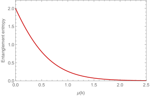
Figure 1: The entanglement entropy $S_{k}$ of the vacuum state $\left|0_{k}0_{-k}\right\rangle$ vs. the parameter $\mu$ given by Eq. (3.6). Considering $m^{2}$ and $E$ to be fixed, $S_{k}$ is maximum in the small $\mu$ ($|B|,n_{L}\ll|E|$, along with our initial condition, $m^{2}/|qE|\ll 1$), where the number of outgoing particle is unity, and vanishing for large $\mu$ ($E\ll n_{L},|B|$), where the number density of outgoing particle is zero. See the text for discussions.

5 Mutual information and logarithmic negativity in systems of two scalar fields

Let us now consider systems which are constructed by two complex scalar fields. There are two species of (anti)particles, which do not interact with each other. The total Hilbert space $\mathcal{H}$ is given by, $\mathcal{H}=\prod_{s,k}\mathcal{H}_{s}\otimes\mathcal{H}_{-s}\otimes\mathcal{H}_{k}\otimes\mathcal{H}_{-k}$, where $s$ and $k$ stand for the two species of scalar fields. We assume that these two scalar fields have the same charge, but different masses are allowed.

We shall focus on the maximally entangled states for the incoming states of the (anti)particles. Now, the gauge transformation properties of the wave function of a charged field in quantum electrodynamics puts a constraint on how one can prepare those states, as follows. The wave functions corresponding to two states with different charge content will have different transformation properties under the local gauge transformation. Hence if we add two or more states to construct an entangled state, we must ensure that the charge content of each of these states are the same, so that the wave function for the full state has a definite transformation property. This will be reflected in the states (5.1) and (5.7) we work with.

5.1 Single-charge state

Based upon the above argument, we consider a maximally entangled single-charge state, $\rho^{(1)}=|\psi_{sk}^{(1)}\rangle\langle\psi_{sk}^{(1)}|$, which is a pure state, with

$$\begin{split}\left|\psi_{sk}^{(1)}\right\rangle&=\frac{\left|0_{s}0_{-s};1_{k}0_{-k}\right\rangle_{\text{in}}+\left|1_{s}0_{-s};0_{k}0_{-k}\right\rangle_{\text{in}}}{\sqrt{2}}\end{split}$$ (5.1)

In our notation, the first (second) pair of entries appearing in the kets stands for the first (second) scalar. For a specific pair, the first (second) entry represents particle (antiparticle).

Using the expansion of the incoming vacuum, (4.3), we rewrite $\left|1_{k}0_{-k}\right\rangle_{\text{in}}={a^{\text{in}}_{k}}^{\dagger}\left|0_{k}0_{-k}\right\rangle_{\text{in}}$ by the outgoing states as

$$\begin{split}\left|1_{k}0_{-k}\right\rangle_{\text{in}}&=\sum_{n=0}^{\infty}C_{n_{k}}^{1}\left|(n+1)_{k}n_{-k}\right\rangle_{\text{out}},\end{split}$$ (5.2)

where the coefficient $C_{n_{k}}^{1}$ is given by

$$\begin{split}C_{n_{k}}^{1}=\frac{\sqrt{n+1}}{\alpha_{k}}C_{n_{k}}^{0}=\left(1-\left|\gamma_{k}\right|^{2}\right)\gamma_{k}^{n}e^{i\theta_{\nu}^{1}},\qquad\qquad\theta_{\nu}^{1}=2\left(\frac{\pi}{4}+\arg{\Gamma(-\nu)})\right)+\phi_{c}\end{split}$$ (5.3)

Here, we are using the label $k$ for $\gamma_{k}$, as it depends on the mass and the charge of the particle with momentum $k$. The features of $C_{n_{k}}^{1}$ are given in parallel with that of $C_{n_{k}}^{0}$ in the preceding section.

The coefficients $C_{n_{k}}^{1}$ depend on only the variable $\mu$, and hence $C_{n_{k}}^{1}$ reflects the charge and the mass but not the momentum $k^{0}$ and $k^{x}$. When $\mu\to\infty$, we obtain $|C_{n_{k}}^{1}|\to\delta_{n0}$, and hence (5.2) becomes $\left|1_{k}0_{-k}\right\rangle_{\text{in}}\to C_{0_{k}}^{1}\left|1_{k}0_{-k}\right\rangle_{\text{out}}$, where the difference between the left- and right-hand side is just a phase factor. When $\mu\to 0$, we have $|C_{n_{k}}^{1}|\to\sqrt{n+1}/2^{(n+2)/2}$.

Also, using the relations (4.3) and (5.2), the single-particle ‘in’ state $|\psi_{sk}^{(1)}\rangle$ can be written in terms of the ‘out’ states, necessary to make the squeezed state expansion.

5.1.1 Quantum Mutual information

Here we compute the quantum mutual information defined in Section 2.2, corresponding to the state in Eq. (5.1). We shall focus on two reduced density matrices that characterise the particle-particle and also the particle-antiparticle correlations between the two scalar fields.

Let us start with the particle-particle correlation. The reduced density matrix is given by $\rho_{s,k}^{(1)}=\mathrm{Tr}_{-s,-k}\rho^{(1)}$ and is written in terms of the ‘out’ states as

$$\begin{split}\rho_{s,k}^{(1)}&=\frac{1}{2}\sum_{n,\ell=0}^{\infty}\biggl{(}C_{\ell_{s}}^{0}C_{n_{k}}^{1}\left|\ell_{s}(n+1)_{k}\right\rangle_{\text{out}}+C_{\ell_{s}}^{1}C_{n_{k}}^{0}\left|(\ell+1)_{s}n_{k}\right\rangle_{\text{out}}\biggr{)}\times\left(\text{h.c.}\right),\end{split}$$ (5.4)

where $(\text{h.c.})$ stands for the Hermitian conjugate of the first parenthesis. In the limit of large $\mu(k)$ and $\mu(s)$, $S(\rho_{s,k}^{(1)})$ vanishes.

The quantum mutual information is defined by $I(\rho_{s,k}^{(1)})=S(\rho_{s}^{(1)})+S(\rho_{k}^{(1)})-S(\rho_{s,k}^{(1)})$, where $\rho_{s}^{(1)}=\mathrm{Tr}_{k}\rho_{sk}^{(1)}$ and $\rho_{k}^{(1)}=\mathrm{Tr}_{s}\rho_{sk}^{(1)}$. The summation in (5.4) converges rapidly and hence for numerical purpose, we replace the infinity with a finite but large $n$- and $\ell$-value. We thus obtain the $\mu$-dependence of $I(\rho_{s,k}^{(1)})$, shown in Fig. 2. Here we have defined

$$\Delta\equiv\mu(s)-\mu(k),$$

reflecting, e.g., the mass difference between the fields. Moreover as we consider various parametric values of $\Delta$, we assume to vary $\mu(s)$ keeping $\mu(k)$ fixed.

Fig. 2 shows that $I(\rho_{s,k}^{(1)})$ approaches its maximum value, $S(\rho_{s}^{(1)})+S(\rho_{k}^{(1)})=2$, as $\mu(k)$ increases, showing the correlation of the particle-particle sector is maximum for the large $\mu$ limit of (5.4). When $\mu$ is small, the lines for the different values of $\Delta$ split, e.g., the mass difference of the two scalar fields can be estimated with fixed $E$ and $B$ in that region. Fig. 2 also implies that the pair-creation disturbs the correlation, which originally exists in terms of the incoming modes.

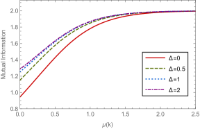
Figure 2: The quantum mutual information of $\rho_{s,k}^{(1)}$ vs. $\mu(k)$ (i.e., the particle-particle sector) for each value of $\Delta$, corresponding to the single charge state in Eq. (5.1). All lines approach $S(\rho_{s}^{(1)})+S(\rho_{k}^{(1)})=2$ as $\mu(k)$ increases. This asympotic value corresponds to the initial state itself, see text for discussion.

Next, we consider correlations of the particle-antiparticle and antiparticle-antiparticle sector. We write the reduced density matrices, $\rho_{\pm s,-k}^{(1)}=\mathrm{Tr}_{\mp s,k}\rho^{(1)}$, in terms of the outgoing modes as

$$\begin{split}\rho_{s,-k}^{(1)}&=\frac{1}{2}\sum_{n,\ell=0}^{\infty}\biggl{(}C_{\ell_{s}}^{0}C_{(n-1)_{k}}^{1}\left|\ell_{s}(n-1)_{-k}\right\rangle_{\text{out}}+C_{\ell_{s}}^{1}C_{n_{k}}^{0}\left|(\ell+1)_{s}n_{-k}\right\rangle_{\text{out}}\biggr{)}\times\left(\text{h.c.}\right),\end{split}$$ (5.5)

$$\begin{split}\rho_{-s,-k}^{(1)}&=\frac{1}{2}\sum_{n,\ell=0}^{\infty}\biggl{(}C_{\ell_{s}}^{0}C_{(n-1)_{k}}^{1}\left|\ell_{-s}(n-1)_{-k}\right\rangle_{\text{out}}+C_{(\ell-1)_{s}}^{1}C_{n_{k}}^{0}\left|(\ell-1)_{-s}n_{-k}\right\rangle_{\text{out}}\biggr{)}\times\left(\text{h.c.}\right),\end{split}$$ (5.6)

with the requirement $C^{1}_{(-1)_{k}}=0$. We also define $\rho_{-k}^{(1)}=\mathrm{Tr}_{s}\rho_{s,-k}^{(1)}$ and $\rho_{-s}^{(1)}=\mathrm{Tr}_{-k}\rho_{-s,-k}^{(1)}$. Note that $\rho_{\pm s,-k}^{(1)}$ becomes a product state $\rho_{\pm s}^{(1)}\otimes\rho_{-k}^{(1)}$ in the limit of large $\mu(k)$ and $\mu(s)$, and consequently the mutual information becomes zero, as discussed in Section. 2.2.

Fig. 3 shows that the mutual information of $\rho_{\pm s,-k}^{(1)}$ approaches zero as $\mu(k)$ increases. This corresponds to the fact, that for large $\mu(k)$ values, the Bogoliubov transformation becomes trivial, and the ‘out’ and ‘in’ states coincide modulo some trivial phase factors, as discussed in Section 5.1. However, (5.1) has no antiparticle content in it, resulting in a vanishing mutual information between the particle-antiparticle (antiparticle-antiparticle) sector in this limit. On the other hand, for smaller $\mu$ values, the lines split as Fig. 2. In addition, we observe that $\rho_{-s,-k}^{(1)}$ shows the inverted hierarchy of $\Delta$ compared to $\rho_{s,\pm k}^{(1)}$.

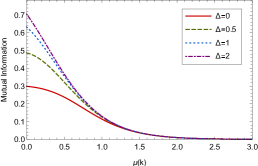
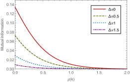
Figure 3: The quantum mutual informations of $\rho_{s,-k}^{(1)}$ (left) and of $\rho_{-s,-k}^{(1)}$ (right) vs. $\mu(k)$ for each value of $\Delta$ (i.e., the particle-antiparticle and antiparticle-antiparticle sector), corresponding to the single charge state in Eq. (5.1). All lines approach zero, since $S(\rho_{\pm s,-k}^{(1)})=S(\rho_{\pm s}^{(1)})+S(\rho_{-k}^{(1)})$ in the limit of large $\mu(k)$. Note the qualitative difference from Fig. 2.

5.1.2 Logarithmic negativity

Let us now compute the logarithmic negativity, first for the particle-particle sector, $\rho_{s,k}^{(1)}$. The $\mu(k)$-dependence of the logarithmic negativity of $\rho_{s,k}^{(1)}$ is shown in Fig. 4 for different values of $\Delta$. The logarithmic negativity increases as $\mu(k)$ increases and for large $\mu(k)$-values, all the lines converge to unity. This is because $\rho_{s,k}^{(1)}$ has the same eigenvalues as that of incoming modes in the large $\mu(k)$ limit, so that $\mathcal{L}_{N}\to\log_{2}\left(4\times{1}/{2}\right)=1$. This behaviour implies that the entanglement of $\rho_{s,k}^{(1)}$ is disturbed by the pair-creation.

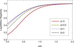
Figure 4: The logarithmic negativities of $\rho_{s,k}^{(1)}$ vs. $\mu(k)$ (i.e. the particle-particle sector) for each value of $\Delta$, corresponding to the single charge state in Eq. (5.1). In the limit of large $\mu(k)$, the logarithmic negativities approach unity. Also, we have not plotted the particle-antiparticle sector, where the logarithmic negativity turns out to be vanishingly small for all $\mu(k)$ values.

For the particle-antiparticle and antiparticle-antiparticle sector, however, we find that the logarithmic negativities are vanishingly small, $\mathcal{L}_{N}(\rho_{\pm s,-k}^{(1)})\lesssim{\cal O}(10^{-15})$, for all $\mu(k)$ values, showing once again the qualitative differences of these sectors with the particle-particle sector.

We shall consider another example of entangled state below and will see the differences between the information quantities associated with it and those of Eq. (5.1).

5.2 Zero-charge state

Keeping in mind the discussion made at the end of Section 5, we now consider a pure state $\rho^{(\text{PA})}=|\psi_{sk}^{(\text{PA})}\rangle\langle\psi_{sk}^{(\text{PA})}|$, where

$$\begin{split}\left|\psi_{sk}^{(\text{PA})}\right\rangle&=\frac{1}{\sqrt{2}}\biggl{(}\left|1_{s}0_{-s};0_{k}1_{-k}\right\rangle_{\text{in}}+\left|0_{s}1_{-s};1_{k}0_{-k}\right\rangle_{\text{in}}\biggr{)},\end{split}$$ (5.7)

has zero net charge content. Let us compute the same measures as earlier in order to see the qualitative differences.

5.2.1 Quantum Mutual information

Using the earlier techniques, we derive the reduced density operator for the particle-particle sector, $\rho_{s,k}^{(\text{PA})}=\mathrm{Tr}_{-s,-k}\rho^{(\text{PA})}$, which is written in terms of the ‘out’ states as

$$\begin{split}\rho_{s,k}^{(\text{PA})}&=\frac{1}{2}\sum_{\ell,n=0}^{\infty}\biggl{(}C_{\ell_{s}}^{1}C_{(n-1)_{k}}^{1}\left|(\ell+1)_{s}(n-1)_{k}\right\rangle_{\text{out}}+C_{(\ell-1)_{s}}^{1}C_{n_{k}}^{1}\left|(\ell-1)_{s}(n+1)_{k}\right\rangle_{\text{out}}\biggr{)}\times\left(\text{h.c.}\right).\end{split}$$ (5.8)

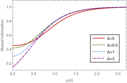
Figure 5: The quantum mutual information of $\rho_{s,k}^{(\text{PA})}$ vs. $\mu(k)$ (i.e., the particle-particle sector) for each value of $\Delta$, corresponding to the particle-antiparticle state in Eq. (5.7).

On the other hand, the reduced density operator for the particle-antiparticle sector is given by

$$\begin{split}\rho_{s,-k}^{(\text{PA})}&=\frac{1}{2}\sum_{n,\ell=0}^{\infty}\biggl{(}C_{\ell_{s}}^{1}C_{n_{k}}^{1}\left|(\ell+1)_{s}(n+1)_{-k}\right\rangle_{\text{out}}+C_{(\ell-1)_{s}}^{1}C_{(n-1)_{k}}^{1}\left|(\ell-1)_{s}(n-1)_{-k}\right\rangle_{\text{out}}\biggr{)}\times\left(\text{h.c.}\right).\end{split}$$ (5.9)

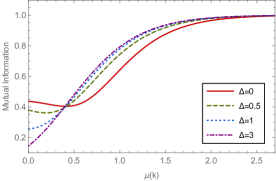
Figure 6: The quantum mutual information of $\rho_{s,-k}^{(\text{PA})}$ vs. $\mu(k)$ (i.e., the particle-antiparticle sector) for each value of $\Delta$, corresponding to the particle-antiparticle state in Eq. (5.7).

The $\mu(k)$-dependence of the quantum mutual information corresponding to the particle-particle sector, Eq. (5.8), and the particle-antiparticle sector, Eq. (5.9), for different values of $\Delta$ is depicted respectively in Fig. 5, Fig. 6. We note the overall qualitative similarity between them, although Fig. 6 shows minimum for $\Delta\to 0$. We also note that the mutual information for both of them have the same numerical orders, unlike those of the single-charge state. These similarities should correspond to the symmetry in particle and antiparticle number of the initial state, Eq. (5.7). Due to the same reason, the antiparticle-antiparticle sector of this state yields exactly the same correlations as those of particle-particle sector, and we do not pursue it any further.

We also note some qualitative difference in the behaviour of Fig. 2 with that of Fig. 5 and Fig. 6: the former has simple feature such as the monotonicity and unchanging hierarchy with respect to $\Delta$, while the latter shows interchanges of the hierarchy and the non-monotonic behaviour in Fig. 6.

5.2.2 Logarithmic negativity

Finally, we compute the logarithmic negativity for the particle-particle and the particle-antiparticle sector by following the methods described earlier. They have respectively been plotted in Fig. 7 and Fig. 8. We note the overall qualitative similarity between them, owing once again to the symmetry in the number of particles and antiparticles in (5.7). The asymptotically vanishing values in the plots for large $\mu(k)$ just as earlier correspond to the fact that in this limit we reach the initial state, Eq. (5.7), and it has no logarithmic negativity, as can be checked easily. The antiparticle-antiparticle sector behaves in the same manner as the particle-particle sector. We also note the qualitative differences of these plots with that of Fig. 4, which arises from the existence of both particle and antiparticle in the incoming zero-charge state.

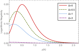
Figure 7: The logarithmic negativity of $\rho_{s,k}^{(\text{PA})}$ vs. $\mu(k)$ (i.e., the particle-particle sector) for each value of $\Delta$, corresponding to the particle-antiparticle state in Eq. (5.7).

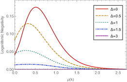
Figure 8: The logarithmic negativity of $\rho_{s,-k}^{(\text{PA})}$ vs. $\mu(k)$ (i.e., the particle-antiparticle sector) for each value of $\Delta$, corresponding to the particle-antiparticle state in Eq. (5.7).

6 Summary and outlook

We now summarise our results. The chief motivation of this work was to quantify the effect of a background magnetic field on the quantum correlations between the Schwinger pairs. We have studied the vacuum entanglement entropy in Section 4, and the quantum mutual information and logarithmic negativity for maximally entangled states with single and zero electric charges respectively in Section 5.1 and Section 5.2. We have emphasised the qualitative differences in the behaviour of the information quantities between these states. Note also that since the number density of created particles equals $|\beta_{k}|^{2}=e^{-\pi\mu}$ (cf. the discussion below Eq. (4.5)), all the plots above will show similar behaviour with respect to $|\beta_{k}|^{2}$ as well. Extension of these results to the Rindler and the inflationary backgrounds seems to be interesting.

Finally, we note that in all the plots the various information quantities converge to some specific points for sufficiently large $\mu(k)$ values. Assuming for example, the mass, the electric field and the Landau level to be fixed, a large $\mu(k)$ corresponds to large values of the magnetic field, Eq. (3.6). In this limit the Bogoliubov transformation becomes trivial and an ‘out’ state becomes coincident with the ‘in’ state, modulo some trivial phase factor (cf., the discussion below Eq. (4.4)). Keeping in mind that the background electric field is analogous to the acceleration parameter in an accelerated frame as far as the particle creation is concerned, it then seems possible that the degraded quantum correlation between two entangled states in such frames, e.g. MartinMartinez:2010ar , might be restored (for charged fields) via the application of a background magnetic field, as follows. The magnetic Lorentz force, $q\vec{v}\times\vec{B}$, acts in the same direction for the particle and antiparticle initially moving in the opposite direction just after the pair creation. An electric field or background spacetime curvature/acceleration do just the opposite effect by moving the created pairs away, e.g. Mironov:2011hp . Thus to the best of our understanding, it seems reasonable to expect that the particle-antiparticle thermal pair creation causing the entanglement degradation in the Rindler frame, will get diminished in the presence of a background magnetic field of an ‘appropriate’ value. As an example, we may consider Fig. 8. The logarithmic negativity, which is a measure of entanglement for a mixed ensemble indeed grows and reaches maximum for certain $\mu$ values. After this point however, the particle creation becomes too weak and the squeezed state expansion coincides with that of the initial state, which itself has vanishing logarithmic negativity. Depending upon the characteristics of the initial state, analogous arguments can be made for all the cases we have investigated in this paper. We hope to come back to this issue in detail in our future work. Such effect can in particular be relevant for a black hole endowed with a strong magnetic field in its exterior.

References

- (1) M. B. Plenio and S. Virmani, An Introduction to entanglement measures, Quant. Inf. Comput. 7, 1 (2007) [quant-ph/0504163].
- (2) R. Horodecki, P. Horodecki, M. Horodecki and K. Horodecki, Quantum entanglement, Rev. Mod. Phys. 81, 865 (2009) [quant-ph/0702225].
- (3) G. Adesso, T. R. Bromley and M. Cianciaruso, Measures and applications of quantum correlations, J. Phys. A 49, no. 47, 473001 (2016) [arXiv:1605.00806 [quant-ph]].
- (4) R. F. Werner, Quantum states with Einstein-Podolsky-Rosen correlations admitting a hidden-variable model, Phys. Rev. A 40, 4277 (1989).
- (5) K. Zyczkowski, P. Horodecki, A. Sanpera and M. Lewenstein, Volume of the set of separable states, Phys. Rev. A 58, 883 (1998) [quant-ph/9804024].
- (6) G. Vidal, Entanglement monotones, J. Mod. Opt. 47, 355 (2000) [arXiv:quant-ph/9807077].
- (7) G. Vidal and R. F. Werner, Computable measure of entanglement, Phys. Rev. A 65, 032314 (2002) [quant-ph/0102117].
- (8) M. B. Plenio, Logarithmic negativity: a full entanglement monotone that is not convex, Phys. Rev. Lett. 95, 090503 (2005)
- (9) P. Calabrese, J. Cardy and E. Tonni, Entanglement negativity in extended systems: A field theoretical approach J. Stat. Mech. 1302, P02008 (2013) [arXiv:1210.5359 [cond-mat.stat-mech]].
- (10) T. Nishioka, Entanglement entropy: holography and renormalization group, Rev. Mod. Phys. 90, no. 3, 035007 (2018) [arXiv:1801.10352 [hep-th]].
- (11) M. A. Nielsen and I. L. Chuang (2010), Quantum Computation and Information Theory (Cambridge university press).
- (12) P. M. Alsing and G. J. Milburn, Teleportation with a uniformly accelerated partner, Phys. Rev. Lett. 91, 180404 (2003) [quant-ph/0302179].
- (13) I. Fuentes-Schuller and R. B. Mann, Alice falls into a black hole: Entanglement in non-inertial frames, Phys. Rev. Lett. 95, 120404 (2005) [arXiv:quant-ph/0410172].
- (14) E. Martin-Martinez, L. J. Garay and J. Leon, xUnveiling quantum entanglement degradation near a Schwarzschild black hole, Phys. Rev. D 82, 064006 (2010) [arXiv:1006.1394 [quant-ph]].
- (15) I. Fuentes, R. B. Mann, E. Martin-Martinez and S. Moradi, Entanglement of Dirac fields in an expanding spacetime Phys. Rev. D 82, 045030 (2010) [arXiv:1007.1569 [quant-ph]].
- (16) Entanglement negativity in the multiverse, JCAP 1503, 015 (2015) [arXiv:1412.2838 [hep-th]].
- (17) J. Martin and V. Vennin, Quantum Discord of Cosmic Inflation: Can we Show that CMB Anisotropies are of Quantum-Mechanical Origin?, Phys. Rev. D93, no. 2, 023505 (2016) [arXiv:1510.04038 [astro-ph.CO]].
- (18) J. Maldacena, A model with cosmological Bell inequalities, Fortsch. Phys. 64, 10 (2016) [arXiv:1508.01082 [hep-th]].
- (19) R. de Putter and O. Dore, In search of an observational quantum signature of the primordial perturbations in slow-roll and ultraslow-roll inflation, Phys. Rev. D 101, no.4, 043511 (2020) [arXiv:1905.01394 [gr-qc]].
- (20) S. Bhattacharya, S. Chakrabortty and S. Goyal, Dirac fermion, cosmological event horizons and quantum entanglement, Phys. Rev. D 101, no.8, 085016 (2020) [arXiv:1912.12272 [hep-th]].
- (21) S. Bhattacharya, S. Chakrabortty and S. Goyal, Emergent -like fermionic vacuum structure and entanglement in the hyperbolic de Sitter spacetime, Eur. Phys. J. C 79, no.9, 799 (2019) [arXiv:1812.07317 [hep-th]].
- (22) A. Matsumura and Y. Nambu, Squeezing of primordial gravitational waves as quantum discord, Universe 6, no.2, 33 (2020) [arXiv:2001.02474 [gr-qc]].
- (23) S. Ryu and T. Takayanagi, Holographic derivation of entanglement entropy from AdS/CFT, Phys. Rev. Lett. 96, 181602 (2006) [hep-th/0603001].
- (24) S. Ryu and T. Takayanagi, Aspects of Holographic Entanglement Entropy, JHEP 0608, 045 (2006) [hep-th/0605073].
- (25) P. Calabrese, J. Cardy and E. Tonni, Entanglement negativity in quantum field theory, Phys. Rev. Lett. 109, 130502 (2012) [arXiv:1206.3092 [cond-mat.stat-mech]].
- (26) P. Calabrese, J. Cardy and E. Tonni, “Finite temperature entanglement negativity in conformal field theory,” J. Phys. A 48, no. 1, 015006 (2015) doi:10.1088/1751-8113/48/1/015006 [arXiv:1408.3043 [cond-mat.stat-mech]].
- (27) M. Rangamani and M. Rota, “Comments on Entanglement Negativity in Holographic Field Theories,” JHEP 1410, 060 (2014) doi:10.1007/JHEP10(2014)060 [arXiv:1406.6989 [hep-th]].
- (28) J. S. Schwinger, On gauge invariance and vacuum polarization, Phys. Rev. 82, 664 (1951).
- (29) L. E. Parker and D. Toms, Quantum Field Theory in Curved Spacetime : Quantized Field and Gravity (Cambridge University Press, Cambridge, UK, 2009)
- (30) Z. Ebadi and B. Mirza, Entanglement Generation by Electric Field Background, Annals Phys. 351, 363 (2014) [arXiv:1410.3130 [quant-ph]].
- (31) Y. Li, Y. Dai and Y. Shi, Pairwise mode entanglement in Schwinger production of particle-antiparticle pairs in an electric field, Phys. Rev. D 95, no.3, 036006 (2017) [arXiv:1612.01716 [hep-th]].
- (32) D. C. Dai, State of a particle pair produced by the Schwinger effect is not necessarily a maximally entangled Bell state, Phys. Rev. D 100, no.4, 045015 (2019) [arXiv:1908.01005 [hep-th]].
- (33) Z. T. Xia, Nonexotic-exotic bipartite mode entanglements of an baryon Nucl. Phys. A 989, 97-116 (2019)
- (34) S. Gavrilov, D. Gitman and A. Shishmarev, States of charged quantum fields and their statistical properties in the presence of critical potential steps, Phys. Rev. A 99, no.5, 052116 (2019) [arXiv:1901.01217 [hep-th]].
- (35) Y. Li, Q. Mao and Y. Shi, Schwinger effect of a relativistic boson entangled with a qubit, Phys. Rev. A 99, no.3, 032340 (2019) [arXiv:1812.08534 [hep-th]].
- (36) D. Karabali, S. Kurkcuoglu and V. Nair, Magnetic Field and Curvature Effects on Pair Production I: Scalars and Spinors, Phys. Rev. D 100, no.6, 065005 (2019) [arXiv:1904.11687 [hep-th]].
- (37) D. Karabali, S. Kurkcuoglu and V. Nair, Magnetic Field and Curvature Effects on Pair Production II: Vectors and Implications for Chromodynamics Phys. Rev. D 100, no.6, 065006 (2019) [arXiv:1905.12391 [hep-th]].
- (38) A. Agarwal, D. Karabali and V. Nair, Gauge-invariant Variables and Entanglement Entropy Phys. Rev. D 96, no.12, 125008 (2017) [arXiv:1701.00014 [hep-th]].
- (39) C. Gabriel and P. Spindel, Quantum charged fields in Rindler space, Annals Phys. 284, 263 (2000) [gr-qc/9912016].
- (40) E. Bavarsad, S. P. Kim, C. Stahl and S. S. Xue, Effect of a magnetic field on Schwinger mechanism in de Sitter spacetime, Phys. Rev. D 97, 025017 (2018) [arXiv:1707.03975 [hep-th]].
- (41) Higher Transcendental Functions, edited by A. Erdlyi and the staff of the Bateman Manuscript Project (McGraw-Hill, New York, 1953), Vol. II, Chap. VIII.
- (42) A. Mironov, A. Morozov and T. Tomaras, Geodesic deviation and particle creation in curved spacetimes, JETP Lett. 94, 795-799 (2012) [arXiv:1108.2821 [gr-qc]].