Self-play Reinforcement Learning for Video Transmission

Abstract.

Video transmission services adopt adaptive algorithms to ensure users’ demands. Existing techniques are often optimized and evaluated by a function that linearly combines several weighted metrics. Nevertheless, we observe that the given function fails to describe the requirement accurately. Thus, such proposed methods might eventually violate the original needs. To eliminate this concern, we propose Zwei, a self-play reinforcement learning algorithm for video transmission tasks. Zwei aims to update the policy by straightforwardly utilizing the actual requirement. Technically, Zwei samples a number of trajectories from the same starting point, and instantly estimates the win rate w.r.t the competition outcome. Here the competition result represents which trajectory is closer to the assigned requirement. Subsequently, Zwei optimizes the strategy by maximizing the win rate. To build Zwei, we develop simulation environments, design adequate neural network models, and invent training methods for dealing with different requirements on various video transmission scenarios. Trace-driven analysis over two representative tasks demonstrates that Zwei optimizes itself according to the assigned requirement faithfully, outperforming the state-of-the-art methods under all considered scenarios.

1. Introduction

Thanks to the dynamic growth of video encoding technologies and basic Internet services (Cisco, 2017), currently we are living with the great help of video transmission services. In particular, the videos are required to transmit with fulfilling users’ requirements, where the requirement is often known as quality of experience (QoE) or quality of service (QoS). Unfortunately, as much as the fundamental issue has already been published about two decades (Mo et al., 1999), current approaches, either heuristics or learning-based methods, fall short of achieving this goal. On the one hand, heuristics often use existing domain knowledge (Mo et al., 1999) as the working principle. However, such approaches sometimes require careful tuning and will backfire under the circumstance that violated with presumptions, finally resulting in the failure of achieving acceptable performance under all considered scenarios. On the other hand, learning-based methods (Mao et al., 2017; Zhang et al., 2019) leverage deep reinforcement learning (DRL) to train a neural network (NN) by interacting with the environments without any presumptions, aiming to obtain higher reward. In recent work, the reward function is often defined as a linear-based equation with the combination of manipulation variables. While in this study, we empirically discover that i) an inaccurate reward function may mislead the learning-based algorithm to generalize bad strategies, since ii) the actual requirement can hardly be presented by the linear-based reward function with fixed weights. Moreover, iii) considering the diversity of real-world network environments, it’s difficult to present an accurate reward function that can perfectly fit any network conditions (§2.2). As a result, despite its abilities to gain higher numerical reward score, learning-based schemes may generalize a strategy that hardly meet the actual requirements.

Taking a look from another perspective, we observe that the aforementioned problem can be naturally described as a deterministic goal or requirement (Huang et al., 2018). For instance, in the most cases, the goal of the adaptive bitrate (ABR) streaming algorithm is to achieve lower rebuffering time first, and next, reaching higher bitrate (Huang et al., 2019; Mao et al., 2019). Inspired by this opportunity, we envision a self-play reinforcement learning-based framework, known as Zwei, which can be viewed as a solution for tackling the video transmission dilemma (§3). The key idea of Zwei is to sample trajectories repeatedly by itself, and distinguish the sequence that is closer to the assigned demand, so as to learn the strategy for satisfying the demand iteratively. Specifically, we apply Monte-Carlo (MC) search to estimate moving decisions from the starting point. In the MC search process, several trajectories are sampled from the starting state according to the current policy. Then the expected long-term win rate is estimated by averaging the competition results from each trajectory pairs, where the result represents which one is closer to the actual demand between the two trajectories. Having estimated the win rate, Zwei adopts the proximate policy optimization (PPO) (Schulman et al., 2017) to optimize the NN via increasing the probabilities of the winning sample and reducing the possibilities of the failure sample.

In the rest of the paper (§4), we attempt to evaluate the potential of Zwei using trace-driven analyses of various representative video transmission scenarios. To achieve this, we build several faithful video transmission simulators which can accurately replicate the environment via real-world network dataset. Specifically, we validate Zwei on two different tasks (§2.1), including client-to-server, and server-to-client service. Note that each of them has individual requirements and challenges. As expected, evaluation results demonstrate the superiority of Zwei against existing state-of-the-art approaches on all tasks. In detail, we show that (i) Zwei outperforms existing ABR algorithms on both HD videos and 4K videos, with the improvements on Elo score (Coulom, 2008) of 32.24% - 36.38%. (ii) In the crowd-sourced live streaming (CLS) scheduling task, Zwei reduces the overall costs on 22% and decreases over 6.5% on the overall stalling ratio in comparison of state-of-the-art learning-based scheduling method LTS (Zhang et al., 2019).

Contributions: This paper makes four key contributions.

• We point out the shortcoming of learning-based schemes in video transmission tasks and present the idea that update networks without reward engineering (§2.2).

• Zwei is a novel framework that aims to employ the self-play reinforcement learning method to make the idea practical (§3).

• We implement Zwei into two representative video transmission scenarios, i.e. rate adaptation and crowd-sourced scheduling. Results indicates that Zwei outperforms existing schemes on all considered scenarios (§4).

2. Background and Challenges

2.1. Video Transmission Services

In this work, the video transmission service mainly consists of:

Client-to-Server Service. In this scenario, users often adopts a video player to watch the video on demand. First, video contents are pre-encoded and pre-chunked as several bitrate ladders on the server. Then the video player, placed on the client side, dynamically picks the proper bitrate for the next chunk to varying network conditions. Specifically, the bitrate decisions should achieve high bitrate and low rebuffering on the entire session (Bentaleb et al., 2018; Huang et al., 2019). We call it adaptive bitrate streaming (ABR).

Server-to-Client Service. Considering that if we were the content provider and currently we had multiple content delivery networks (CDNs) with different costs and performance, how to schedule the users’ requests to the proper CDN, aiming to provide live streaming services withing less stalling ratio and lower cost? In common, we call that crowd-sourced live streaming(CLS) (Zhang et al., 2019).

Details of each video transmission scenario are demonstrated in §4. We can see that the video transmission task is often required to obtain better performance under various mutual metrics.

2.2. Challenges

Motivation. Recent video transmission algorithms mainly consist of two types, i.e., heuristics and learning-based scheme. Heuristic methods utilize an existing fixed model or domain knowledge to construct the algorithm, while they inevitably fail to achieve optimal performance in all considered network conditions due to the inefficient parameter tuning (§5,(Mao et al., 2017)). Learning-based schemes train a NN model towards the higher reward score from scratch, where the reward function is often defined as a linear combination of several weighted metrics (Zhang et al., 2019; Mao et al., 2017). Nevertheless, considering the characteristics of the video transmission tasks above, we argue that the policy generated by the linear-based reward fails to always perform on the right track. We, therefore, set up two experiments in the ABR scenario (4.2) to prove this conjecture.

Figure 1. We show average bitrate and rebuffering time for each ABR method. ABRs are performed over the HSDPA network traces.

Observation 1. The best learning-based ABR algorithm Pensieve (Mao et al., 2017) is not always the best scheme on every network traces.

Recently, given a deterministic QoE metric with linearly combining of several underlying metrics, several attempts have been made to propose the ABR algorithm via model-based (Yin et al., 2015) or model-free reinforcement learning (RL) method (Mao et al., 2017). However, such method heavily relies on the accuracy of the given QoE metric. Especially, how to set a proper QoE parameter for each network condition is indeed a critical challenges for training a good ABR algorithm. In order to verify whether QoE parameters have influenced the performance of ABR algorithms, we set up an experiment to report average bitrate and rebuffering time of several state-of-the-art ABR baselines (§4.2.3) and Zwei. Despite the outstanding performances that Pensieve achieves, the best learning-based ABR algorithm does not always stand for the best scheme. On the contrary, Zwei always outperforms existing approaches.

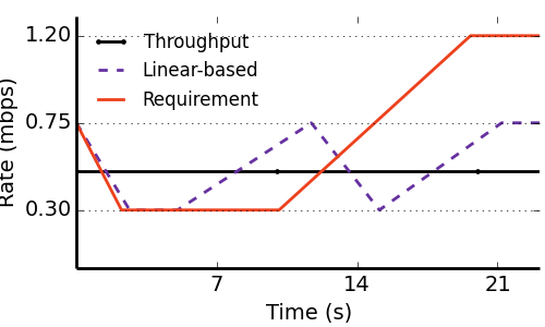
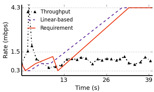
Figure 2. The comparison of linear-based optimal and requirement-based optimal strategy. Results are evaluated on fixed (0.5mbps) and the real-world network trace (Riiser et al., 2013). We can see the difference between the actual requirement and the optimal trajectory generated by the linear-based reward.

Observation 2. Recent linear-based weighted reward function can hardly map the actual requirement for all the network traces.

To better understand the effectiveness of weighted-sum-based reward functions, we compare the optimal strategy of linear-based with requirement-based under two representative network traces, in which linear-based optimal is the policy which obtains maximum reward, and the requirement-based optimal stands for the closest strategy in terms of the given requirement. Unsurprisingly, from Figure 2 we observe that linear-based optimal policy performs differently compared with the requirement-based optimal strategy. The reason is that the given weighted parameters are not allowed to be adjusted dynamically according to the current network status. Generally, we believe that the policy learned by reward engineering might fall into the unexpected conditions.

Summary. In general, we observe that no matter how precisely and carefully the parameter of the linear-based reward function tunes, such tuned functions can hardly meet the requirement of any network conditions. E.g., the parameter of stable and unstable network conditions are not the same. To that end, traditional learning-based scheme, which often optimizes the NN via the assigned functions, will eventually fail to provide a reliable performance on any network traces. We therefore, attempt to learn the strategies from the original demands.

3. Zwei Design

In this section, we briefly introduce the details of Zwei, including its key principle, training algorithms and implementation details.

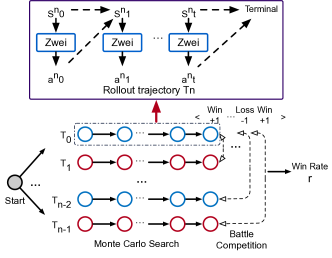
Figure 3. Zwei System Overview. The framework is mainly composed of four phases: Monte Carlo sampling, battle competition, win rate estimation, and policy optimization.

3.1. Basic Idea

As mentioned before, we attempt to generalize the strategy based on actual requirements instead of linear-based reward functions. Considering the basic requirement seldom directly provides gradients for optimization, we, therefore, employ the self-play method (Silver et al., 2016) that enables the NN to explore better policies and suitable rewards via self-learning. Zwei treats the learning task as a competition between distinct trajectories sampled by itself, where the competition outcome is determined by a set of rules, symbolizing which one is closer to the given requirement. Subsequently, we are able to update the NN towards achieving a better outcome.

3.2. Training Methodology

Figure 3 presents the main phases in our framework. The pipeline can be summarized as follows:

Phase1: Monte Carlo Sampling. First, we adopt MC sampling method to sample $N$ different trajectories $T_{n}=\{s_{0}^{n},a_{0}^{n},s_{1}^{n},a_{1}^{n},$ $\dots,a_{t}^{n}\},n\in N$ w.r.t the given policy $\pi(s)$ under the same environments ($a_{t}\sim\pi(s_{t})$) and start point (the gray point in Figure 3). Next, we record and analysis the underlying metric for the entire session. Finally, we store all the sample $T_{n}$ into $D$. Note that we can select Monte Carlo Tree Search (MCTS) (Silver et al., 2016), which is widely used in advanced research, to implement the process.

Phase2: Battle Competition. To better estimate how the current policy performs, Zwei requires a module to label all trajectories from $D$: given two different trajectories, $T_{i}$ and $T_{j}$ which are all collected from the same environment settings ($T_{i},T{j}\in D$)), we attempt to identify which trajectory is positive for NN updating, and which trajectory is generated by the worse policy. Thus, we implement a rule called Rule which can determine the better trajectory between the given two candidates, in which better means which trajectory is closer to the requirement. At the end of the session, the terminal position $s_{t}$ is scored w.r.t the rules of the requirement for computing the game outcome $o$: $-1$ for a loss, $0$ for a draw, and $+1$ for a win. The equation is listed in Eq. 1.

(1) $$o_{i}^{j}=\texttt{Rule}(T_{i},T_{j}).$$

(2) $$s.t.\quad o_{i}^{j}=\{-1,0,1\},T_{i},T_{j}\in D,T_{i}\neq T_{j}.$$

Phase3: Win Rate Estimation. Next, having computed the competition outcome $o_{i}$ for any two trajectories, we then attempt to estimate the average win rate $r_{i}$ for each trajectory $T_{i}$ in $D$, i.e., $r_{i}=\mathbb{E}[\texttt{Rule}(T_{i},)]=\lim_{N\to\infty}\frac{1}{N}\sum_{u}^{N}o_{i}^{u}$. Notice that the accuracy of the win rate estimation heavily depends on the number $N$ of trajectories. Since it’s impractical to sample infinite number of samples in the real world, we further list the performance comparison of different sample numbers in §4.2.

Phase4: Policy Optimization.  In this part, given a batch of collected samples and their win rate, our key idea is to update the policy via elevating the probabilities of the winning sample from the collected trajectories and diminishing the possibilities of the failure sample from the worse trajectories. In other words, the improved policy $\pi$ at state $s_{t}$ is required to pick the action $a_{t}$ which produced the best estimated win rate $r_{t}$. We employ Proxy Policy Optimization (PPO) (Schulman et al., 2017), a state-of-the-art actor-critic method, as to optimize the NN’s policy. PPO uses clip method to restrict the step size of the policy iteration and update the NN by minimizing the following clipped surrogate objective. We list the Zwei’s loss function $\mathcal{L}^{\text{Zwei}}(\theta)$ in Eq. (6). The function consists of a policy loss and a outcome loss. The policy are computed as Eq. 3, where $p_{t}(\theta)$ denote the probability ratio between the policy $\pi_{\theta}$ and the old policy $\pi_{\theta_{\text{old}}}$, i.e., $\frac{\pi_{\theta}(a_{t}|s_{t})}{\pi_{\theta_{\text{old}}}(a_{t}|s_{t})}$; $\epsilon$ is the hyper-parameters which controls the clip range. We set $\epsilon=0.2$ which consistent with the original paper (Schulman et al., 2017). $\hat{A}_{t}$ is the advantage function (Eq. 4), $V_{\theta_{p}}(s)$ is provided by another value NN. Meanwhile, the value loss aims to minimize the mean square error between $r_{t}$ and $V_{\theta_{p}}(s)$ (Eq. 5). Moreover, we also add entropy $H(s_{t};\theta)$ to encourage exploration. For more details, please refer to our repository (Huang, 2020).

(3) $$\mathcal{L}^{\emph{Policy}} =\hat{\mathbb{E}_{t}}\Big{[}\min\Big{(}p_{t}(\theta)\hat{A}_{t},\text{clip}\big{(}p_{t}(\theta),1-\epsilon,1+\epsilon\big{)}\hat{A}_{t}\Big{)}\Big{]}.$$

(4) $$\hat{A}_{t}=r_{t}-V_{\theta_{p}}(s_{t})$$

(5) $$\mathcal{L}^{\emph{Value}}=\frac{1}{2}\hat{\mathbb{E}_{t}}\left[V_{\theta_{p}}(s_{t})-r_{t}\right]^{2}.$$

(6) $$\nabla\mathcal{L}^{Zwei}=\nabla_{\theta}\mathcal{L}^{\emph{Policy}}+\nabla_{\theta_{p}}\mathcal{L}^{\emph{Value}}+\nabla_{\theta}\beta H(s_{t};\theta).$$

4. Evaluation

In this section, we thoroughly evaluate the performance of Zwei over two representative scenarios.

4.1. Zwei’s NN Implementation

We use TensorFlow (Abadi et al., 2016) to construct Zwei. Zwei’s policy network takes a n-dims vector with softmax active function as the output, and the outcome network outputs a value with tanh function scaled in $(-1,1)$. Considering the characteristics on video transmission tasks, we construct different NN architectures for each task, but use the same set of hyper-parameters for training the NN: sample number $N=16$, learning rate $\alpha=10^{-4}$. Notice that we discuss the NN architecture and the effect of different sample number in §4.2.

4.2. ABR Scenarios

4.2.1. ABR’s Background

The ABR video streaming architecture consists of a video player client with a constrained buffer length and an HTTP-Server or Content Delivery Network (CDN). The video player client decodes and renders video frames from the playback buffer. Once the streaming service starts, the client fetches the video chunk from the HTTP Server or CDN orderly by an ABR algorithm. The algorithm determines next chunks’ video quality. After finished to play the video, several metrics, such as total bitrate, total re-buffering time and total bitrate change will be summarized as a QoE metric to evaluate the performance.

(a) Zwei vs. ABR schemes

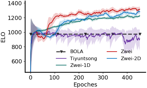
(b) Zwei vs. Tiyuntsong

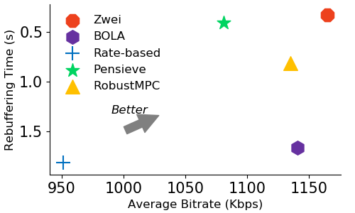
(c) ABR Scheme Details

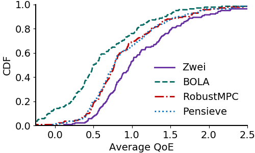
(d) CDF of ABR Algorithms

Figure 4. This group of figures show the comparison results of Zwei and other ABR approaches. Results are evaluated in the typical ABR system with HD Videos (video resolution=1920 $\times$ 1080, maximum bitrate=4.3mbps).

4.2.2. NN Architecture

We now explain the details of the Zwei’s neural network (NN), including its inputs, outputs, network architecture, and implementation.

Inputs. For each chunk $k=8$, Zwei takes the state inputs $S_{k}=\{X_{k},\tau_{k},N_{k},b_{k},c_{k},l_{k}\}$ as the input, in which $X_{k}$ represents the throughput measured for past $t$ times, $\tau_{k}$ reflects the vector of download time for past $t$ chunks, $N_{k}$ is the next video sizes for each bitrate chunk, $b_{k}$ means current buffer occupancy, $l_{k}$ is the normalized value of the last bitrate selected, $c_{k}$ is the scalar which means the video chunk remaining.

Outputs. We attempt to use discrete action space to describe the output. Note that the output is an n-dim vector indicating the probability of the bitrate being selected under the current ABR state $S_{k}$. In this work, we set $n=6$, which is widely used in ABR papers (Huang et al., 2018; Mao et al., 2017).

NN Representation. Zwei’s NN representation is quite simple: it leverages three fully-connected layers, which is sized 128, 64, and 64 respectively, for describing the feature extraction layer. The output of the NN’s policy network is a 6-dims vector, which represents the probabilities for each bitrate selected. The NN’s outcome network outputs a value scaled in (-1, 1).

Requirements for ABR tasks. Algorithm 1 is an example of Rule Rule which used in the ABR scenario, where $\epsilon_{c}$ is a small number that can add noise for improving Zwei’s robustness. In this work, we set $\epsilon_{c}$ as 10. Note that, such settings are trivial and you can just set the value as a small value (e.g., 0.1) instead.

Algorithm 1 Rule for the ABR task.

1:Trajectory $T_{u},T_{v}$;

2:Compute average bitrate $r_{u},r_{v}$, average rebuffering $b_{u},b_{v}$ from the given trajectories $T_{u},T_{v}$. $\triangleright$ Requirements: i) low rebuffering time ii) high bitrate.

3:Initialize Return $s=\{-1,-1\}$;

4:if $\left|b_{u}-b_{v}\right|<\epsilon_{c}$ or $\left|r_{u}-r_{v}\right|<\epsilon_{c}$ then

5:    Randomly set $s_{0}$ or $s_{1}$ as 1. $\triangleright$ Add noise to improve the robustness.

6:else if $\left|b_{u}-b_{v}\right|<\epsilon_{c}$ then

7:    $s_{i}\leftarrow 1,i={argmax}_{i\in\{u,v\}}{r}$;

8:else

9:    $s_{i}\leftarrow 1,i={argmin}_{i\in\{u,v\}}{b}$;

10:end if

11:return $s$;

QoE Representation. Recall that the goal of ABR algorithm is to select bitrates for the next chunk $k$ with high bitrate $r_{k}$ and less rebuffering time $t_{k}$ (Mao et al., 2019), thus the optimization reward $q_{k}$ can be normally written as $q_{k}=r_{k}-\alpha t_{k}$, here $\alpha$ is the coefficient that adjust the importance of the underlying metrics. Note that prior research often add additional smoothness metric $\left|r_{k}-r_{k-1}\right|$ to control the bitrate change of the entire session, while in practice the following metric is neglectable for the ABR algorithm (Mao et al., 2019; Huang et al., 2019). Hence, in this work we also set the smoothness to zero for better understanding the fundamental performance of Zwei. Solving Zwei with smoothness metric will be our future work.

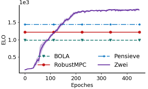
(a) Zwei vs. ABR schemes

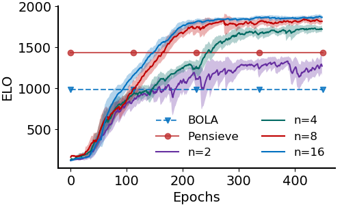
(b) Zwei with Different Samples

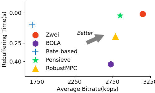
(c) ABR Algorithm Details

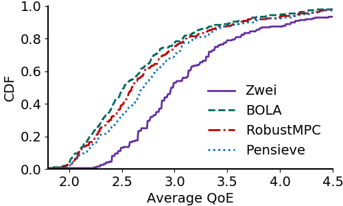
(d) CDF of ABR Algorithms

Figure 5. This group of figures show the comparison results of Zwei and other ABR approaches. Results are evaluated in the typical ABR system with 4K Videos (video resolution=3840 $\times$ 2160, maximum bitrate=12.0mbps).

4.2.3. Experimental Setup

We employ the standard ABR’s emulation environment (Mao et al., 2017) to evaluate Zwei. We adopt various network bandwidth databases, including HSDPA (Riiser et al., 2013), FCC (Report, 2016). Training process lasts approximate 45000 steps, within 10 hours to obtain a reliable result. In this experiment, we setup two ABR scenarios, i.e., HD and 4K video scenario. In the HD video scenario, we adopt EnvivioDash3, a video that commonly used in recent work (Mao et al., 2017), to validate Zwei, where the video chunks are encoded as $\{0.3,0.75,1.2,1.8,2.8,4.3\}$ mbps. In the 4K-video scenario, we use the popular open-source movie Big Buck Bunny (bbb, 2020), which is now even more a world standard for video standards. Specifically, we pick 6 bitrates from Dash.js standard (das, 2019), i.e., $\{0.2,0.6,1.5,4.0,8.0,12.0\}$ mbps.

ABR Baselines. In this paper, we select several representational ABR algorithms from various type of fundamental principles:

1. Rate-based (Jiang et al., 2014): the basic baseline for ABR problems. It leverages harmonic mean of past five throughput measured as future bandwidth.

2. BOLA (Spiteri et al., 2016): the most popular buffer-based ABR scheme in practice. BOLA turns the ABR problem into a utility maximization problem and solve it by using the Lyapunov function.

3. RobustMPC (Yin et al., 2015): a state-of-the-art heuristic method which maximizes the objectives by jointly considered the buffer occupancy and throughput predictions. We implement RobustMPC by ourselves.

4. Pensieve (Mao et al., 2017): the state-of-the-art learning-based ABR scheme which utilizes DRL to select bitrate for next video chunks.

5. Tiyuntsong (Huang et al., 2018): the first study of multi-objective optimization ABR approach. Tiyuntsong uses actor-critic method to update the NN via the competition with two agents under the same network condition.

Evaluation Metrics The Elo rating (Coulom, 2008) is a traditional method for calculating the relative performance of players in zero-sum games. It’s suitable to compare different schemes via win rate information only. Thus, we also use Elo score to compare different ABR schemes, similar to that of AlphaGo (Silver et al., 2016) and Tiyuntsong (Huang et al., 2018).

4.2.4. HD Video

We study the performance of Zwei over the HD video dataset and HSDPA network traces. Followed by recent work (Yin et al., 2015), we set $\alpha$ = 4.3 as the basic QoE-HD metric.

Zwei vs. Existing schemes.  In this experiment, we compare Zwei with existing ABR schemes over the HSDPA dataset. Results are computed as the Elo-score and reported in Figure 4(a). Specifically, we first select several previously proposed approaches and validate the performance respectively under the same network and video environment. Next, we use Rule to estimate their winning rate. Finally, we compute the Elo rating for these approaches.

Through the experiments we can see that Zwei outperforms recent ABR approaches. In particular, Zwei improves Elo-score on 36.38% compared with state-of-the-art learning-based method Pensieve, and increases 31.11% in terms of state-of-the-art heuristic method RobustMPC. Same conclusion are demonstrated as the CDF of QoE in Figure 4(d). Besides, we also illustrate the comparison results of different methods on average bitrate and average rebuffering in Figure 4(c). As shown, Zwei can not only achieve highest bitrate but also obtain lowest rebuffering under all network traces. We compare Zwei with previously proposed self-learning method Tiyuntsong on the same experimental setting. Results are shown as the Elo-curve in Figure 4(b). As expected, Zwei with any NN architectures outperforms Tiyuntsong on average Elo-score of 35%. The reason is that Tiyuntsong treat the learning process as a battle with two separated NNs, as each agent have to use the sample only collected by the agent itself. Thus, it lacks sample efficiency and sometimes struggles into the sub-optimal solution.

Zwei with Different NN Architectures. This experiment considers Zwei with several NN architectures, where Zwei-1D is the standard ABR NN architecture (Mao et al., 2017), Zwei-2D uses stacked Conv-2D layers to extract features, and Zwei takes three fully-connected layers sized $\{128,64,64\}$. Results are shown in Figure 4(b). Unsurprisingly, when Zwei trains with some complicated NN architecture (i.e., Zwei-1D and Zwei-2D), it performs worse than the fully connected NN scheme. This makes sense since ABR is a light-weighted task which can be solved in a practical and uncomplicated manner instead of a NN incorporating some deep yet wide layers.

4.2.5. 4K Video

we evaluate Zwei with 4K videos on HDFS network traces, and the video are encoded with $\{0.2,0.6,1.5,4.0,8.0,12.0\}$ mbps. In particular, we have also retrained Pensieve with the Big Buck Bunny and QoE-4K.

QoE metrics for other approaches. Due to the difference between the maximum bitrate of 4K video (i.e., 12mbps) and HD video (i.e., 4.3mbps), we refer $QoE_{4}K$ as the QoE function for other ABRs (expect Zwei). Specifically, we set the penalty of rebuffering parameter $\alpha$ to 20 for better avoiding the occurrence of rebuffering.

Zwei vs. Recent ABR Schemes. Figure 5(a) plots the learning curves in terms of the comparison of Zwei and other ABR methods. We observe that Zwei has already achieved state-of-the-art performance in almost 200 epochs, and finally, the performance improvement of Zwei can achieve 32.24% against the second best algorithm Pensieve and 58.58%-120.76% against others. What’s more, as depicted in Figure 5(c), no matter average bitrate or total rebuffering time, Zwei always stands for the best scheme among all candidates. In particular, Zwei increases 10.46% on average bitrates with reducing 56.52% on total rebuffering time. Meanwhile, we also report the comparison of QoE performance of the proposed scheme in Figure 5(d). As expected, Zwei outperforms existing ABR algorithms without reward engineering, with the increasing on average QoE of 11.59%.

Zwei with Different Samples $N$. Besides, we also investigate the Elo-rating of Zwei with different sample $N$, where we set $N=\{2,4,8,16\}$. Figure 5(b) illustrates the comparison of each method, we observe that Zwei can achieve sample efficiency with the increasing of the sample number $N$.

4.3. CLS Scheduling

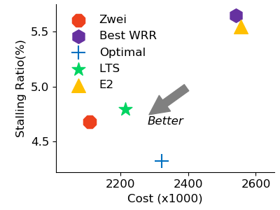
(a) Zwei vs. Existing Methods

(b) Zwei Training Curve

Figure 6. Results of Zwei under the CLS environment.

4.3.1. CLS Overview

The ClS system is composed of a source server and several CDNs. Upon received viewers’ requests, the CLS platform will first aggregate all stream data to the source server, and then deliver the video stream to viewers through CDN providers according to a certain scheduling strategy.

4.3.2. Implementation

Our experiments are conducted on the real-world CLS dataset provided by the authors (Zhang et al., 2019), spanning 1 week (6 days for training and 1 day for test). At each time, we select 3 candidates from total 4 different CDN providers, and we fit a separate simulator for them. Followed by previous work (Zhang et al., 2019), we use a piecewise linear model to characterize this relationship between workload and block ratio. Note that the following features are extracted by the real CDN dataset. What’s more, we set the CDN pricing model w.r.t various CDN providers in industry, such as Amazon E2 and Tencent CDN. See (Huang, 2020) for details.

Algorithm 2 Rule for the CLS task.

1:Trajectory $T_{u},T_{v}$;

2:Compute average stalling ratio ${stall}_{u},{stall}_{v}$, accumulative cost $c_{u},c_{v}$ from the given trajectories $T_{u},T_{v}$. $\triangleright$ Requirements: i) low stalling ratio ii) low costs.

3:Initialize Return $s=\{-1,-1\}$;

4:if $\left|{stall}_{u}-{stall}_{v}\right|<\epsilon$ or $\left|c_{u}-c_{v}\right|<\epsilon_{c}$ then

5:    Randomly set $s_{0}$ or $s_{1}$ as 1. $\triangleright$ Add noise to improve the robustness.

6:else if $\left|{stall}_{u}-{stall}_{v}\right|<\epsilon_{c}$ then

7:    $s_{i}\leftarrow 1,i={argmin}_{i\in\{u,v\}}{c}$;

8:else

9:    $s_{i}\leftarrow 1,i={argmin}_{i\in\{u,v\}}{stall}$;

10:end if

11:return $s$;

Baselines. Like other scenarios, we also compare Zwei with the following state-of-art scheduling baselines:

1. Weighted round robin (WRR) (Adhikari et al., 2012). The requests will be redirected to different CDN providers w.r.t a constant ratio. We adopt the algorithm with the best parameters.

2. E2 (Jiang et al., 2017). Exploitation and Exploration (E2) algorithm utilizes harmonic mean for estimating CDN providers’ performance, and select with the highest upper confidence bound of reward. We use E2 algorithm provided by the authors (Jiang et al., 2017).

3. LTS (Zhang et al., 2019). State-of-the-art CLS algorithm which uses deep reinforcement learning to train the NN towards lower stalling ratio. However, it ignores the trade-off between the cost and the performance. We evaluate LTS by Zhang et. al. (Zhang et al., 2019).

NN Representation. We implement Zwei in CLS as suggested by recent work (Zhang et al., 2019). More precisely speaking, for each CDN provider $i$, Zwei passes past 20 normalized workload and stalling ratio into Conv-2D layers with filter=64, size=4, and stride=1. Then several output layers are merged into a hidden layer that uses 64 units to apply the softmax activation function. We model the action space as a heuristic way: each CDN provider has 3 choices, i.e., incrementally increases its configuration ratio by 1%, 5%, and 10%.

Requirements for CLS tasks. Algorithm 2 describes the Rule of CLS. Note that the $\epsilon_{c}=10$ is also a small number that can add noise to improve Zwei’s robustness.

Zwei vs. State-of-the-art Scheduling Methods We start to study how well that Zwei achieves under the CLS scenario. As shown in Figure 6(a), we find that Zwei stands for the best scheme among the candidates. Specifically, Zwei reduces the overall costs on 22% compared with state-of-the-art learning-based method LTS, and decreases over 6.5% in terms of the overall stalling ratio. The reason is that LTS takes the weight-sumed combination function as the reward, while the function can hardly give a clearer guidance for the optimized algorithm. Moreover, comparing the performance of Zwei with the optimal strategy generated by the reward function, we observe that both optimal policy and Zwei are in the Pareto front. Zwei consumes less pricing costs than the optimal policy since the requirement is to minimize the cost first.

Details. Besides, we also present the training process in Figure 6(b). As shown, Zwei converges in less than 600 epochs, which needs about 3 hours. It’s worth noting that Zwei also experienced two stages on the CLS task. The first stage ranges from 0 to 100 epochs, and we can see the goal of Zwei is to minimize the cost without considering the number of stalling ratio. The rest of the process we find that Zwei attempts to reduce the number of stalling ratio. Meanwhile, the cost curve converges to a steady state.

5. Related Work

Heuristic Methods. Heuristic-based ABR methods often adopts throughput prediction (E.g., FESTIVE (Jiang et al., 2014)) or buffer occupancy control (E.g., BOLA (Spiteri et al., 2016)) to handle the task. However, such approaches suffer from either inaccurate bandwidth estimation or long-term bandwidth fluctuation problems. Then, MPC (Yin et al., 2015) picks next chunks’ bitrate by jointly considering throughput and buffer occupancy. Nevertheless, MPC is sensitive to its parameters since the it relies on well-understanding different network conditions.

Through preliminary measurements, it is widely accepted that the strategies are largely statically configured (Adhikari et al., 2012). In recent years, dynamic scheduling across different CSPs has received more attention. Jiang et. al. (Jiang et al., 2017) uses E2 method to replace traditional model-based methods.

Learning-based Schemes. Recent years, several learning-based attempts have been made to tackle video transmission problem. For example, Mao et al. (Mao et al., 2017) develop an ABR algorithm that uses DRL to select next chunks’ bitrate. Tiyuntsong optimizes itself towards a rule or a specific reward via the competition with two agents under the same network condition (Huang et al., 2018). LTS (Zhang et al., 2019) is a DRL-based scheduling approach which outperforms previously proposed CLS approaches. However, such methods fail to achieve actual requirements since they are optimized via a linear-based reward function.

6. Conclusion

We propose Zwei, which utilize self-play RL to enhance itself based on the actual requirement, where the requirement is always hard to be described as a linear-based manner. We show that Zwei outperforms recent work with the improvements of more than 22% on two representative video transmission tasks.  (32.24% on Elo score over the ABR scenario, 22% on stalling ratio over the LTS).

Acknowledgement. We thank the MMSys and NOSSDAV reviewer for the valuable feedback. This work was supported by NSFC under Grant 61936011, 61521002, Beijing Key Lab of Networked Multimedia, and National Key R&D Program of China (No. 2018YFB1003703).

Appendix A Appendix

This supplementary material details the principle of Zwei. Due to the length of the supplemental material, we list a content to facilitate the selection of interested parts for review. Although these contents have NOT appeared in the main text, we believe that they will help the reviewer get a thorough understanding of Zwei.

A.1. Additional Experiments for ABR Tasks

We list the experimental details under validation set from Table 1 to Table 3, where the ABR algorithm includes Zwei, BOLA, RobustMPC, Pensieve and Rate-based. The validation set contains several different network scenarios. E.g., bus-1 represents network trace No.1 which collected from the bus.

Table 1. Details of ABR Tasks

Trace Name	BOLA		Rate-based		Pensieve		RobustMPC		Zwei
-	Avg. Bit.	Rebuf.	Avg. Bit.	Rebuf.	Avg. Bit.	Rebuf.	Avg. Bit.	Rebuf.	Avg. Bit.	Rebuf.
bus 1	2659.6	-	2188.3	-	2480.9	-	2839.4	5.1	2802.1	-
bus 10	1467.0	-	1389.4	4.6	1413.8	-	1427.7	0.1	1490.4	-
bus 11	1327.7	-	1195.7	-	1264.9	-	1336.2	0.6	1363.8	-
bus 12	769.1	4.9	721.3	-	771.3	5.2	769.1	4.0	793.6	-
bus 13	852.1	9.7	529.8	-	623.4	2.6	629.8	5.5	666.0	0.7
bus 14	1675.5	8.3	933.0	-	1586.2	4.6	1610.6	4.6	1638.3	-
bus 15	3919.1	-	3497.9	-	3598.9	-	4141.5	-	3888.3	-
bus 16	3950.0	-	3652.1	-	3857.4	-	4145.7	-	3897.9	-
bus 17	1943.6	-	1844.7	2.2	1777.7	-	2005.3	-	2022.3	-
bus 18	1623.4	-	1559.6	0.4	1596.8	-	1588.3	1.0	1643.6	-
bus 19	1472.3	-	1212.8	-	1461.7	-	1440.4	-	1517.0	-
bus 2	1820.2	-	1656.4	-	1737.2	-	1861.7	-	1919.1	-
bus 20	1726.6	-	1517.0	1.6	1703.2	-	1752.1	-	1795.7	-
bus 21	1669.1	-	1497.9	-	1526.6	-	1759.6	2.1	1730.9	-
bus 22	1743.6	-	1594.7	7.8	1568.1	-	1791.5	3.6	1806.4	3.3
bus 23	1176.6	2.3	985.1	11.7	1076.6	-	1195.7	4.3	1178.7	-
bus 3	1331.9	-	1258.5	-	1283.0	-	1348.9	0.9	1368.1	-
bus 4	2121.3	-	1710.6	-	2103.2	-	2160.6	1.2	2156.4	-
bus 5	950.0	1.9	863.8	14.0	922.3	-	964.9	-	966.0	-
bus 6	1568.1	-	1324.5	0.3	1520.2	-	1606.4	-	1680.9	-
bus 7	2669.1	-	2376.6	-	2460.6	-	2571.3	-	2668.1	-
bus 8	2230.9	-	2008.5	2.9	2093.6	-	2305.3	-	2290.4	-
bus 9	2192.6	-	2014.9	4.0	2079.8	-	2297.9	1.8	2283.0	-
car 1	1440.4	0.8	1413.8	10.1	1467.0	12.7	1447.9	4.0	1434.0	-
car 10	1300.0	-	1127.7	-	1218.1	-	1338.3	2.6	1350.0	-
car 11	920.2	1.7	673.4	1.0	925.5	-	889.4	-	969.1	-
car 12	1291.5	18.2	1283.0	6.4	1291.5	13.7	1308.5	24.9	1325.5	13.5
car 2	1029.8	-	903.2	-	996.8	-	1034.0	-	1060.6	-
car 3	1351.1	1.8	1293.6	-	1334.0	2.0	1309.6	0.8	1327.7	-
car 4	1433.0	1.6	1327.7	3.4	1314.9	-	1423.4	1.7	1476.6	-
car 5	927.7	2.1	836.2	0.1	878.7	-	895.7	-	959.6	-
car 6	1295.7	-	1133.0	-	1263.8	-	1286.2	-	1326.6	-
car 7	710.6	1.3	568.1	11.9	666.0	-	677.7	0.9	697.9	-
car 8	1688.3	-	1448.9	-	1676.6	-	1704.3	-	1748.9	-
car 9	1485.1	-	1366.0	-	1423.4	-	1459.6	-	1526.6	-
ferry 1	1454.3	0.3	1423.4	-	1441.5	-	1455.3	-	1492.6	-
ferry 10	1119.1	0.2	1021.3	0.2	1104.3	0.2	1104.3	0.2	1133.0	0.2
ferry 11	1038.3	1.2	847.9	-	978.7	-	1037.2	0.1	1067.0	-
ferry 12	1525.5	-	1324.5	6.4	1466.0	-	1555.3	-	1586.2	-
ferry 13	1421.3	0.5	1192.6	12.6	1320.2	-	1436.2	5.4	1471.3	1.8
ferry 14	2036.2	-	1850.0	0.3	2074.5	-	2098.9	-	2124.5	-
ferry 15	1551.1	-	1385.1	-	1535.1	-	1486.2	1.1	1573.4	-
ferry 16	2684.0	-	2406.4	-	2480.9	-	2734.0	-	2817.0	-
ferry 17	859.6	0.1	768.1	9.4	818.1	-	826.6	-	850.0	-
ferry 18	724.5	2.8	587.2	4.9	666.0	1.1	667.0	1.0	684.0	-
ferry 19	839.4	4.8	654.3	-	826.6	-	825.5	-	863.8	7.1
ferry 2	1012.8	3.3	951.1	10.6	990.4	-	1001.1	-	1024.5	-

Table 2. Details of ABR Tasks

Trace Name	BOLA		Rate-based		Pensieve		RobustMPC		Zwei
Trace Name	Avg. Bit.	Rebuf.	Avg. Bit.	Rebuf.	Avg. Bit.	Rebuf.	Avg. Bit.	Rebuf.	Avg. Bit.	Rebuf.
ferry 20	686.2	6.7	635.1	-	670.2	5.8	672.3	5.0	674.5	-
ferry 3	1211.7	-	1093.6	-	1170.2	-	1231.9	0.7	1252.1	-
ferry 4	562.8	4.2	472.3	1.9	543.6	-	558.5	4.7	563.8	-
ferry 5	1011.7	1.7	901.1	12.0	940.4	-	1018.1	2.2	1027.7	-
ferry 6	2014.9	-	1598.9	-	2039.4	-	2093.6	-	2119.1	-
ferry 7	1367.0	0.5	1231.9	1.4	1309.6	-	1346.8	0.6	1422.3	-
ferry 8	1078.7	3.8	1010.6	-	1076.6	1.7	1078.7	2.5	1105.3	-
ferry 9	964.9	3.8	787.2	5.1	868.1	3.7	898.9	1.9	1004.3	3.3
metro 1	1350.0	-	1141.5	-	1269.1	-	1371.3	-	1389.4	-
metro 10	896.8	-	625.5	3.7	837.2	-	895.7	-	935.1	-
metro 2	1364.9	-	1285.1	2.8	1316.0	-	1381.9	2.5	1409.6	-
metro 3	934.0	-	481.9	-	884.0	-	913.8	-	956.4	-
metro 4	1086.2	1.0	884.0	1.2	968.1	0.6	1030.9	-	1121.3	-
metro 5	1178.7	1.0	1041.5	3.8	1142.6	-	1171.3	-	1229.8	0.5
metro 6	577.7	0.9	386.2	6.6	558.5	-	548.9	-	573.4	-
metro 7	945.7	-	769.1	-	948.9	0.2	961.7	0.1	977.7	-
metro 8	740.4	2.5	443.6	6.4	738.3	-	724.5	-	762.8	-
metro 9	788.3	-	702.1	4.4	735.1	-	788.3	1.5	806.4	-
train 1	1028.7	4.2	863.8	2.3	996.8	-	1008.5	-	1024.5	-
train 10	1838.3	-	1627.7	-	1709.6	-	1894.7	-	1907.4	-
train 11	1256.4	0.4	1163.8	0.2	1171.3	-	1257.4	-	1286.2	-
train 12	1304.3	0.8	911.7	1.3	1114.9	-	1212.8	-	1380.9	-
train 13	1560.6	-	1236.2	-	1334.0	-	1564.9	-	1675.5	-
train 14	1330.9	-	1206.4	-	1259.6	-	1320.2	-	1356.4	-
train 15	1900.0	-	1423.4	-	1650.0	-	1952.1	-	1944.7	-
train 16	1661.7	-	1475.5	3.5	1484.0	-	1575.5	-	1736.2	-
train 17	1620.2	-	1394.7	4.1	1556.4	-	1637.2	-	1706.4	-
train 18	1978.7	-	1725.5	-	1803.2	-	2012.8	-	2091.5	-
train 19	1423.4	-	1230.9	2.5	1302.1	-	1452.1	-	1484.0	-
train 2	635.1	3.5	481.9	11.1	577.7	-	581.9	-	664.9	3.0
train 20	1331.9	-	1052.1	-	1343.6	-	1357.4	-	1373.4	-
train 21	1598.9	-	1421.3	-	1596.8	-	1626.6	-	1652.1	-
train 3	648.9	1.6	529.8	8.6	619.1	-	596.8	-	629.8	-
train 4	1084.0	3.3	868.1	-	1024.5	-	1059.6	0.3	1127.7	-
train 5	1241.5	1.5	946.8	0.4	1155.3	-	1151.1	-	1283.0	-
train 6	969.1	0.9	721.3	-	875.5	-	936.2	0.9	991.5	-
train 7	825.5	8.3	750.0	-	784.0	-	790.4	-	823.4	2.6
train 8	706.4	1.0	510.6	-	666.0	-	693.6	-	730.9	-
train 9	855.3	-	596.8	-	776.6	-	852.1	-	881.9	-
tram 1	635.1	-	472.3	1.6	625.5	-	635.1	-	656.4	-
tram 10	869.1	2.5	673.4	-	850.0	-	878.7	-	871.3	-
tram 11	587.2	4.3	472.3	1.3	558.5	-	548.9	-	580.9	-
tram 12	807.4	-	548.9	-	795.7	-	816.0	-	826.6	-
tram 13	788.3	-	596.8	0.9	739.4	-	787.2	-	831.9	-
tram 14	839.4	2.2	644.7	1.1	808.5	-	797.9	-	844.7	-
tram 15	453.2	6.9	357.4	5.3	414.9	1.8	424.5	-	437.2	-
tram 16	683.0	-	548.9	-	673.4	-	692.6	-	692.6	-
tram 17	654.3	-	424.5	-	625.5	-	635.1	-	663.8	-
tram 18	730.9	2.8	587.2	-	691.5	-	706.4	-	751.1	-

Table 3. Details of ABR Tasks

Trace Name	BOLA		Rate-based		Pensieve		RobustMPC		Zwei
Trace Name	Avg. Bit.	Rebuf.	Avg. Bit.	Rebuf.	Avg. Bit.	Rebuf.	Avg. Bit.	Rebuf.	Avg. Bit.	Rebuf.
tram 19	967.0	0.1	788.3	-	907.4	-	973.4	-	985.1	-
tram 2	577.7	3.3	434.0	-	548.9	-	548.9	-	559.6	-
tram 20	930.9	-	730.9	-	885.1	-	928.7	-	988.3	-
tram 21	692.6	0.5	558.5	-	677.7	-	696.8	-	711.7	-
tram 22	510.6	0.3	376.6	-	491.5	-	501.1	-	506.4	-
tram 23	778.7	-	529.8	-	738.3	-	778.7	-	808.5	-
tram 24	788.3	-	616.0	3.4	739.4	-	769.1	0.3	808.5	-
tram 25	907.4	-	711.7	-	813.8	-	888.3	-	950.0	-
tram 26	568.1	0.8	300.0	-	539.4	-	568.1	-	567.0	-
tram 27	692.6	-	491.5	-	673.4	-	692.6	-	698.9	-
tram 28	558.5	0.3	386.2	2.2	510.6	-	539.4	-	540.4	-
tram 29	510.6	3.4	338.3	-	481.9	-	501.1	-	495.7	-
tram 3	577.7	1.3	414.9	-	539.4	-	534.0	1.9	570.2	1.7
tram 30	692.6	-	319.1	-	644.7	-	687.2	-	719.1	-
tram 31	769.1	-	644.7	-	753.2	-	769.1	-	783.0	-
tram 32	788.3	-	558.5	1.7	733.0	-	750.0	-	788.3	-
tram 33	874.5	-	644.7	-	841.5	-	877.7	0.2	880.9	-
tram 34	926.6	-	778.7	1.6	917.0	-	930.9	-	959.6	-
tram 35	548.9	5.0	405.3	1.6	501.1	-	486.2	-	550.0	-
tram 36	850.0	0.3	539.4	-	819.1	-	816.0	-	874.5	-
tram 37	984.0	-	807.4	-	894.7	-	1003.2	-	1026.6	-
tram 38	644.7	9.6	481.9	4.5	591.5	-	625.5	4.9	646.8	2.3
tram 39	855.3	-	721.3	-	814.9	-	826.6	-	868.1	-
tram 4	462.8	5.2	300.0	-	414.9	-	414.9	-	428.7	-
tram 40	797.9	0.6	520.2	0.6	770.2	0.6	772.3	0.8	827.7	0.6
tram 41	769.1	2.8	663.8	-	734.0	-	750.0	0.5	785.1	-
tram 42	1069.1	9.0	692.6	-	961.7	-	1057.4	-	1076.6	-
tram 43	1079.8	-	960.6	0.2	1048.9	-	1084.0	-	1105.3	-
tram 44	869.1	-	759.6	-	801.1	-	874.5	0.7	893.6	-
tram 45	648.9	1.1	472.3	7.0	627.7	0.5	635.1	0.5	627.7	0.5
tram 46	683.0	4.2	414.9	-	606.4	-	662.8	0.1	679.8	-
tram 47	788.3	0.9	539.4	-	705.3	-	764.9	-	795.7	-
tram 48	616.0	0.3	395.7	-	558.5	-	605.3	0.2	619.1	-
tram 49	963.8	1.1	778.7	-	963.8	-	985.1	2.2	1007.4	-
tram 5	654.3	5.2	443.6	2.6	587.2	-	616.0	-	640.4	-
tram 50	863.8	6.8	797.9	-	851.1	-	845.7	-	864.9	-
tram 51	658.5	5.5	587.2	-	638.3	-	647.9	-	674.5	4.6
tram 52	920.2	3.4	788.3	1.7	905.3	-	903.2	-	927.7	-
tram 53	657.4	17.3	443.6	3.8	434.0	0.2	428.7	-	522.3	-
tram 54	1123.4	6.8	862.8	6.6	1059.6	-	1109.6	-	1106.4	-
tram 55	1176.6	0.4	1100.0	-	1141.5	-	1146.8	1.9	1177.7	-
tram 56	971.3	-	797.9	-	944.7	-	957.4	-	992.6	-
tram 6	740.4	-	587.2	-	683.0	-	744.7	-	784.0	-
tram 7	759.6	-	596.8	-	720.2	-	744.7	-	797.9	-
tram 8	501.1	3.5	414.9	-	472.3	-	462.8	0.2	483.0	-
tram 9	606.4	0.2	328.7	-	568.1	-	572.3	-	629.8	-

References

- (1)
- das (2019) 2019. DASH Industry Forum — Catalyzing the adoption of MPEG-DASH. (2019). https://dashif.org/
- bbb (2020) 2020. Big Buck Bunny. (Jan 2020). http://www.bigbuckbunny.org
- Abadi et al. (2016) Martín Abadi, Paul Barham, Jianmin Chen, Zhifeng Chen, Andy Davis, Jeffrey Dean, Matthieu Devin, Sanjay Ghemawat, Geoffrey Irving, Michael Isard, et al. 2016. TensorFlow: A System for Large-Scale Machine Learning.. In OSDI, Vol. 16.
- Adhikari et al. (2012) Vijay Kumar Adhikari, Yang Guo, Fang Hao, Matteo Varvello, Volker Hilt, Moritz Steiner, and Zhi-Li Zhang. 2012. Unreeling netflix: Understanding and improving multi-cdn movie delivery. In INFOCOM’12.
- Bentaleb et al. (2018) Abdelhak Bentaleb, Bayan Taani, Ali C Begen, Christian Timmerer, and Roger Zimmermann. 2018. A Survey on Bitrate Adaptation Schemes for Streaming Media over HTTP. IEEE Communications Surveys & Tutorials (2018).
- Cisco (2017) Cisco. 2017. Cisco Visual Networking Index: Forecast and Methodology, 2016-2021. (2017). https://www.cisco.com/c/dam/en/us/solutions/collateral/service-provider/visual-networking-index-vni/complete-white-paper-c11-481360.pdf
- Coulom (2008) Rémi Coulom. 2008. Whole-history rating: A Bayesian rating system for players of time-varying strength. In International Conference on Computers and Games. Springer, 113–124.
- Huang (2020) Tianchi Huang. 2020. Zwei. https://github.com/thu-media/Zwei. (2020).
- Huang et al. (2018) Tianchi Huang, Xin Yao, Chenglei Wu, Rui-Xiao Zhang, and Lifeng Sun. 2018. Tiyuntsong: A Self-Play Reinforcement Learning Approach for ABR Video Streaming. arXiv preprint arXiv:1811.06166 (2018).
- Huang et al. (2019) Te-Yuan Huang, Chaitanya Ekanadham, Andrew J. Berglund, and Zhi Li. 2019. Hindsight: Evaluate Video Bitrate Adaptation at Scale. In MMSys’19 (MMSys ’19). ACM, New York, NY, USA, 86–97. https://doi.org/10.1145/3304109.3306219
- Jiang et al. (2014) Junchen Jiang, Vyas Sekar, and Hui Zhang. 2014. Improving fairness, efficiency, and stability in http-based adaptive video streaming with festive. TON 22, 1 (2014).
- Jiang et al. (2017) Junchen Jiang, Shijie Sun, Vyas Sekar, and Hui Zhang. 2017. Pytheas: Enabling Data-Driven Quality of Experience Optimization Using Group-Based Exploration-Exploitation.. In NSDI, Vol. 1.
- Mao et al. (2019) Hongzi Mao, Shannon Chen, Drew Dimmery, Shaun Singh, Drew Blaisdell, Yuandong Tian, Mohammad Alizadeh, and Eytan Bakshy. 2019. Real-world Video Adaptation with Reinforcement Learning. (2019).
- Mao et al. (2017) Hongzi Mao, Ravi Netravali, and Mohammad Alizadeh. 2017. Neural adaptive video streaming with pensieve. In Proceedings of the Conference of the ACM Special Interest Group on Data Communication. 197–210.
- Mo et al. (1999) Jeonghoon Mo, Richard J La, Venkat Anantharam, and Jean Walrand. 1999. Analysis and comparison of TCP Reno and Vegas. In INFOCOM’99, Vol. 3.
- Report (2016) Measuring Fixed Broadband Report. 2016. Raw Data Measuring Broadband America 2016. https://www.fcc.gov/reports-research/reports/measuring-broadband-america/raw-data-measuring-broadband-america-2016. (2016). [Online; accessed 19-July-2016].
- Riiser et al. (2013) Haakon Riiser, Paul Vigmostad, Carsten Griwodz, and Pål Halvorsen. 2013. Commute path bandwidth traces from 3G networks: analysis and applications. In Proceedings of the 4th ACM Multimedia Systems Conference.
- Schulman et al. (2017) John Schulman, Filip Wolski, Prafulla Dhariwal, Alec Radford, and Oleg Klimov. 2017. Proximal policy optimization algorithms. arXiv preprint arXiv:1707.06347 (2017).
- Silver et al. (2016) David Silver, Aja Huang, Chris J Maddison, et al. 2016. Mastering the game of Go with deep neural networks and tree search. nature 529, 7587 (2016).
- Spiteri et al. (2016) Kevin Spiteri et al. 2016. BOLA: Near-optimal bitrate adaptation for online videos. In INFOCOM’16.
- Yin et al. (2015) Xiaoqi Yin, Abhishek Jindal, Vyas Sekar, and Bruno Sinopoli. 2015. A control-theoretic approach for dynamic adaptive video streaming over HTTP. In SIGCOMM’15.
- Zhang et al. (2019) Rui-Xiao Zhang, Tianchi Huang, Ming Ma, Haitian Pang, Xin Yao, Chenglei Wu, and Lifeng Sun. 2019. Enhancing the crowdsourced live streaming: a deep reinforcement learning approach. In NOSSDAV’19.