Data-driven efficient solvers for Langevin dynamics on manifold in high dimensions

Abstract.

We study the Langevin dynamics of a physical system with manifold structure $\mathcal{M}\subset\mathbb{R}^{p}$ based on collected sample points $\{\mathbf{x}_{i}\}_{i=1}^{n}\subset\mathcal{M}$ that probe the unknown manifold $\mathcal{M}$. Through the diffusion map, we first learn the reaction coordinates $\{\mathbf{y}_{i}\}_{i=1}^{n}\subset\mathcal{N}$ corresponding to $\{\mathbf{x}_{i}\}_{i=1}^{n}$, where $\mathcal{N}$ is a manifold diffeomorphic to $\mathcal{M}$ and isometrically embedded in $\mathbb{R}^{\ell}$ with $\ell\ll p$. The induced Langevin dynamics on $\mathcal{N}$ in terms of the reaction coordinates captures the slow time scale dynamics such as conformational changes in biochemical reactions. To construct an efficient and stable approximation for the Langevin dynamics on $\mathcal{N}$, we leverage the corresponding Fokker-Planck equation on the manifold $\mathcal{N}$ in terms of the reaction coordinates $\mathbf{y}$. We propose an implementable, unconditionally stable, data-driven finite volume scheme for this Fokker-Planck equation, which automatically incorporates the manifold structure of $\mathcal{N}$. Furthermore, we provide a weighted $L^{2}$ convergence analysis of the finite volume scheme to the Fokker-Planck equation on $\mathcal{N}$. The proposed finite volume scheme leads to a Markov chain on $\{\mathbf{y}_{i}\}_{i=1}^{n}$ with an approximated transition probability and jump rate between the nearest neighbor points. After an unconditionally stable explicit time discretization, the data-driven finite volume scheme gives an approximated Markov process for the Langevin dynamics on $\mathcal{N}$ and the approximated Markov process enjoys detailed balance, ergodicity, and other good properties.

1. Introduction

1.1. Problem set up and goals

We study a complex chemical, biological or physical system $P$ which can be described by $p$-dimensional variables $\mathbf{x}$ in $\mathbb{R}^{p}$ with $p\gg 1$. Due to some equality and inequality constraints, we assume the essential structure of the system $P$ is an unknown $d$ dimensional closed smooth Riemannian submanifold $\mathcal{M}$ of $\mathbb{R}^{p}$ [15, 14]. The manifold $\mathcal{M}$ is unknown in the sense that we do not know the charts and the metric of $\mathcal{M}$. The essential physical motions in the system $P$ are those slow time scale structural changes or conformational changes rather than the fast time scale motions such as vibrations. Therefore, despite the high dimensionality of $P$ in practice, we can find some intrinsic low dimensional variables, called reaction coordinates, to represent those essential structural or conformational changes in a low dimensional space [15, 14, 48]. For instance, a typical one dimensional reaction coordinate is the distance between a carbon center and a nucleophile in an $\text{S}_{\text{N}}2$ reaction (one simple nucleophilic substitution reaction mechanism); see also the conformational transitions of alanine dipeptide representing by two backbone dihedral angles [28]. There are many other collective physical/chemical quantities, such as bond length/angle, dihedral angles, and intermolecular distance, that can be used as the reaction coordinates to represent the whole process of conformational transitions or chemical reactions. Mathematically, the reaction coordinates should be a smooth embedding $\mathbf{y}=\Phi(\mathbf{x}):\mathcal{M}\hookrightarrow\mathbb{R}^{\ell}$ with $\ell\ll p$ to preserve the topological structure of the underlying manifold. Then, $\mathcal{N}=\Phi(\mathcal{M})$ is a submanifold of $\mathbb{R}^{\ell}$ with the metric induced by the Euclidean metric of $\mathbb{R}^{\ell}$. The reaction coordinates can be realized through the nonlinear dimension reduction algorithms [45]. Suppose $\{\mathbf{x}_{i}\}_{i=1}^{n}$ are $n$ data points well distributed on the unknown manifold $\mathcal{M}\subset\mathbb{R}^{p}$, while these $n$ points are collected by some sampling methods. A nonlinear dimension reduction algorithm constructs an embedding $\Phi$ by using the coordinates of $\{\mathbf{x}_{i}\}_{i=1}^{n}$ in $\mathbb{R}^{p}$ so that we can present the high dimensional data $\{\mathbf{x}_{i}\}_{i=1}^{n}\subset\mathcal{M}\subset\mathbb{R}^{p}$ as $\mathbf{y}_{i}=\Phi(\mathbf{x}_{i})\subset\mathcal{N}\subset\mathbb{R}^{\ell}$ in the low dimensional space.

We assume the dynamics for the physical system $P$ can be described by a continuous strong Markov process on $\mathcal{M}\subset\mathbb{R}^{p}$. Particularly, the simplest and widely used physical model is the following over-damped Langevin dynamics with a drift determined by some potentials $U$ on $\mathcal{M}$:

(1.1) $$\,\mathrm{d}{\mathbf{x}_{t}}=-\nabla_{\mathcal{M}}U(\mathbf{x}_{t})\,\mathrm{d}t+\sqrt{2kT}\,\mathrm{d}_{\mathcal{M}}B_{t}.$$

We explain the notations in (1.1) below. Let $\{\tau^{\mathcal{M}}_{i};\,1\leq i\leq d\}$ be an orthonormal basis of the tangent plane $T_{\mathbf{x}_{t}}\mathcal{M}$. Denote $\nabla_{\mathcal{M}}:=\sum_{i=1}^{d}\tau^{\mathcal{M}}_{i}\nabla_{\tau^{\mathcal{M}}_{i}}=\sum_{i=1}^{d}\tau^{\mathcal{M}}_{i}\otimes\tau^{\mathcal{M}}_{i}\nabla$ as the surface gradient and $\nabla_{\tau^{\mathcal{M}}_{i}}=\tau^{\mathcal{M}}_{i}\cdot\nabla$ as the tangential derivative in the direction of $\tau^{\mathcal{M}}_{i}$. Let $k$ be the Boltzmann constant, $T$ be the temperature [20] and $\,\mathrm{d}_{\mathcal{M}}B_{t}$ be a Brownian motion on $\mathcal{M}$. This Brownian motion on manifold can be realized by the projection of the standard Brownian motion $B_{t}$ in the ambient space $\mathbb{R}^{p}$:

(1.2) $$\,\mathrm{d}_{\mathcal{M}}B_{t}:=\sum_{i=1}^{d}\tau^{\mathcal{M}}_{i}(\mathbf{x}_{t})\otimes\tau^{\mathcal{M}}_{i}(\mathbf{x}_{t})\circ\,\mathrm{d}B_{t},$$

where $\circ$ is understood in the Stratonovich sense in the stochastic integral [35, p.19, p.78]. We refer the readers to [3] for the general Langevin SDEs on Riemannian manifolds.

The potential $U(\mathbf{x})$ is also known as the energy landscape for the physical system $P$, which is usually very complicated and indicates all the possible (meta)stable states of a physical system. For instance, in a simple nucleophilic substitution reaction mechanism, the states of reactants and products are two stable states in the energy landscape [20]. A saddle point state on the energy landscape is called the transition state, whose value determines the energy barrier in a chemical reaction. In this paper, we assume the output of the potential $U$ at each data point $\{\mathbf{x}_{i}\}_{i=1}^{n}$ is known. The equilibrium of this system $P$, also known as the invariant probability density measure, is $\rho_{\infty}(\mathbf{x})\propto e^{-\frac{U(\mathbf{x})}{kT}},\,\mathbf{x}\in\mathcal{M}$.

Suppose we learn the reaction coordinates $\mathbf{y}=\Phi(\mathbf{x}),\mathbf{x}\in\mathcal{M}$. The diffeomorphism $\Phi:\mathcal{M}\to\mathcal{N}$ induces a map $\Phi_{*}$ from the space $\Gamma(T\mathcal{M})$ of the smooth vector fields on $\mathcal{M}$ to the space $\Gamma(T\mathcal{N})$ of the smooth vector fields on $\mathcal{N}$ such that for any $f\in C^{\infty}(\mathcal{N})$ and $V\in\Gamma(T\mathcal{M})$

(1.3) $$(\Phi_{*}V)f(\mathbf{y})=V(f\circ\Phi)(\mathbf{x}),\quad\mathbf{y}=\Phi(\mathbf{x}).$$

The Stratonovich formulation transforms consistently under diffeomorphism $\Phi$ [35, p. 20]. Notice $\tau^{\mathcal{N}}_{i}\in\mathbb{R}^{\ell}$ is defined by the induced map $\Phi_{*}$ and $B_{t}$ is the $\ell$-dimensional Brownian motion. Therefore, instead of considering (1.1) on $\mathcal{M}$ directly, we consider the SDE on $\mathcal{N}$

(1.4) $$\,\mathrm{d}{\mathbf{y}_{t}}=-\nabla_{\mathcal{N}}U_{\mathcal{N}}(\mathbf{y}_{t})\,\mathrm{d}t+\sqrt{2kT}\sum_{i=1}^{d}\tau^{\mathcal{N}}_{i}(\mathbf{y}_{t})\otimes\tau^{\mathcal{N}}_{i}(\mathbf{y}_{t})\circ\,\mathrm{d}B_{t},$$

where $\nabla_{\mathcal{N}}:=\sum_{i=1}^{d}\tau^{\mathcal{N}}_{i}\nabla_{\tau^{\mathcal{N}}_{i}}=\sum_{i=1}^{d}\tau^{\mathcal{N}}_{i}\otimes\tau^{\mathcal{N}}_{i}\nabla$ is the surface gradient, $\nabla_{\tau^{\mathcal{N}}_{i}}=\tau^{\mathcal{N}}_{i}\cdot\nabla$ is the tangential derivative in the direction of $\tau^{\mathcal{N}}_{i}$, and $U_{\mathcal{N}}$ is the induced potential on manifold $\mathcal{N}$ by the composition

(1.5) $$U_{\mathcal{N}}(\mathbf{y}):=U(\mathbf{x})=U(\Phi^{-1}(\mathbf{y})).$$

The main goal of this paper is to accurately simulate the induced Langevin dynamics (1.4) in terms of the reaction coordinates $\mathbf{y}$ and the information of the potential $U$. To simulate the SDE (1.4) on $\mathcal{N}$ without exact manifold information, one of the most natural ways is to construct an approximated stochastic process on the points $\{\mathbf{y}_{i}\}_{i=1}^{n}$. However, the standard Euler–Maruyama method on manifold can not provide a stable simulation. Hence, our strategy for constructing a stochastic process over $\{\mathbf{y}_{i}\}_{i=1}^{n}$ is described as follows: (i) we detour to approximate the corresponding Fokker-Planck equation on the manifold with a finite volume scheme; (ii) we construct an approximated Voronoi tessellation associated with $\{\mathbf{y}_{i}\}_{i=1}^{n}$; (iii) we construct the transition probability and the jump rate from the finite volume scheme.

By Ito’s formula, the SDE (1.4) gives the following Fokker-Planck equation, which is the governing equation for the density $\rho^{\mathcal{N}}_{t}:=\rho^{\mathcal{N}}(\mathbf{y},t)$,

(1.6) $$\partial_{t}\rho^{\mathcal{N}}_{t}=\text{div}_{\mathcal{N}}(kT\nabla_{\mathcal{N}}\rho^{\mathcal{N}}_{t}+\rho^{\mathcal{N}}_{t}\nabla_{\mathcal{N}}U_{\mathcal{N}})=:\text{FP}^{\mathcal{N}}\rho^{\mathcal{N}}_{t},$$

where $\text{div}_{\mathcal{N}}$ is the surface divergence defined as $\text{div}_{\mathcal{N}}\xi=\sum_{i=1}^{d}\tau_{i}^{\mathcal{N}}\cdot\nabla_{\tau_{i}^{\mathcal{N}}}\xi.$ One equivalent form of (1.6) is the relative entropy formulation

(1.7) $$\partial_{t}\rho^{\mathcal{N}}_{t}=kT\text{div}_{\mathcal{N}}\left(e^{-\frac{U_{\mathcal{N}}}{kT}}\nabla_{\mathcal{N}}(\rho^{\mathcal{N}}_{t}e^{\frac{U_{\mathcal{N}}}{kT}})\right)=\text{FP}^{\mathcal{N}}\rho^{\mathcal{N}}_{t}.$$

Then the main issue is to simulate the Fokker-Planck equation (1.6) on $\mathcal{N}$ whose solution $\rho^{\mathcal{N}}_{t}(\mathbf{y})$ drives any initial density $\rho^{\mathcal{N}}_{0}$ to the invariant measure $\rho^{\mathcal{N}}_{\infty}(\mathbf{y})\propto e^{-\frac{U_{\mathcal{N}}(\mathbf{y})}{kT}}$. After designing a finite volume scheme for the Fokker-Planck equation (1.6) on $\mathcal{N}$, we construct an approximated transition probability and jump rate from it. This approximated Markov process on the manifold automatically incorporates both the manifold structure and the equilibrium information. It enables some implementable data-driven computations on the manifold such as finding the optimal cluster-cluster coarse-grained network, cf. [16, 19, 37, 40, 50, 47] and finding the transition path and energy landscape of chemical reactions, cf. [23, 21, 43, 22, 28, 33, 31, 32].

1.2. Practical difficulties and mathematical implementations

The first difficulty is that we are not able to acquire all the information about the system $P$. Hence, we assume that we can sample $n$ points $\{\mathbf{x}_{i}\}_{i=1}^{n}$ from $\mathcal{M}$ based on a density function on $\mathcal{M}$ with lower and upper bounds so that the data points are well distributed on $\mathcal{M}$. In Section 2, we first show that the diffusion map can approximate an embedding $\Phi$ of the manifold $\mathcal{M}$. Then, we apply the diffusion map algorithm [15] on $\{\mathbf{x}_{i}\}_{i=1}^{n}$ to find the reaction coordinates so that we have $\{\mathbf{y}_{i}=\Phi(\mathbf{x}_{i})\}_{i=1}^{n}\subset\mathcal{N}=\Phi(\mathcal{M})\subset\mathbb{R}^{\ell}$. Note that $\{\mathbf{y}_{i}\}_{i=1}^{n}$ can also be regarded as the samples based on a density function on $\mathcal{N}$ with lower and upper bounds.

Next, we focus on simulating the Fokker-Planck equation (1.6) with a given equilibrium potential $U_{\mathcal{N}}(\mathbf{y})$. To find the trajectory $\rho_{t}^{\mathcal{N}}$, we need to solve the Fokker-Planck equation on the manifold $\mathcal{N}\subset\mathbb{R}^{\ell}$. Our method uses the data points $\{\mathbf{y}_{i}\}_{i=1}^{n}\subset\mathcal{N}$ to construct a discrete approximation of the Fokker-Planck equation (1.6). It is proved that the data points are well-distributed on $\mathcal{N}$ whenever the points are sampled based on a density function with lower and upper bounds [55, 41]. Hence, we can construct a “regularly shaped” Voronoi tessellation on $\mathcal{N}$ from $\{\mathbf{y}_{i}\}_{i=1}^{n}\subset\mathcal{N}$. With the help of such Voronoi tessellation, we introduce a finite volume scheme by applying the relative entropy formulation and finite volume method to (1.6). The finite volume scheme assigns a transition probability and a jump rate for an approximated Markov process on $\{\mathbf{y}_{i}\}_{i=1}^{n}$, i.e., random walk between the nearest neighbor points. In Section 3.2, we prove all the good properties of the approximated Markov process on $\{\mathbf{y}_{i}\}_{i=1}^{n}$ including detailed balance, ergodicity, $L^{1}$-contraction and $\chi^{2}$-divergence dissipation law.

To obtain an implementable finite volume scheme, an approximated Voronoi tessellation associated with $\{\mathbf{y}_{i}\}_{i=1}^{n}$ needs to be constructed with high accuracy. By using the Euclidean coordinates of $\{\mathbf{y}_{i}\}_{i=1}^{n}$, each Voronoi cell can be approximated by a polygon in a tangent space of $\mathcal{N}$; see Section 3.4 for detailed error estimates for the approximated cell volume and face area. Therefore, an approximated transition probability based on the volume of each polygon and the areas of its faces can be assigned over $\{\mathbf{y}_{i}\}_{i=1}^{n}$ and leads to an implementable finite volume scheme (3.80) for the Fokker-Planck equation (1.6); see Section 3 and Theorem 3.14 for consistence and convergence analysis for this implementable finite volume scheme. We also provide an unconditionally stable explicit time descretization for the finite volume scheme based on the detailed balance property of the Markov process in Section 3.5. This explicit scheme is very efficient and enjoys a mass conservation law, unconditional maximum principle and exponential convergence to equilibrium. At last, to show the accuracy of the finite volume scheme, we simulate challenging numerical examples including datasets on a dumbbell, a Klein bottle and a sphere in Section 4.

The approximated transition probability between the nearest neighbor points for the Markov process on $\{\mathbf{y}_{i}\}_{i=1}^{n}\subset\mathcal{N}$ reveals the manifold structure and enables us to efficiently conduct computations such as clustering, coarse-graining and finding the minimal energy path on the manifold. Notice this transition probability between the nearest neighbor points not only incorporates the manifold information but also gives an adapted graph network on the manifold.

The remaining part of the paper will be organized as follows. In Section 2, we use diffusion map to learn the reaction coordinates $\mathbf{y}$. In Section 3, we propose a data-driven solver for the Fokker-Planck equation on manifold $\mathcal{N}$, which assigns an approximated transition probability and a jump rate for an approximated Markov process on $\{\mathbf{y}_{i}\}_{i=1}^{n}$. In Section 4, we also provide several simulation results for the Fokker-Planck dynamics on manifolds learned from point clouds. All the technical lemmas are provided in Appendix for completeness. All the commonly used notations are listed in Table 1 for the sake of clarity.

Table 1. Commonly used notations in this paper.

$Symbols$	$Meaning$
$\mathbb{R}^{p}$, $\mathbb{R}^{\ell}$	High (low) dimensional ambient spaces
$d$	Dimension of the Riemannian manifolds
$\mathcal{M}$, $\mathcal{N}$	$d$-dimensional smooth closed Riemannian submanifolds of the Euclidean spaces
$\mathbf{x}$, $\mathbf{y}$	Points on $\mathcal{M}$ and $\mathcal{N}$ respectively
$dV_{\mathcal{M}}$, $dV_{\mathcal{N}}$	Volume forms on $\mathcal{M}$ and $\mathcal{N}$ respectively
$\Delta$	Laplace Beltrami operator of a manifold
$\lambda_{i}$, $\psi_{i}$	The eigenvalues and the corresponding orthonormal (in $L^{2}$) eigenfunctions of $\Delta$
$\Phi$	Reaction coordinates (Smooth embedding of a manifold)
$X$, $Y$	Random variables with the range $\mathcal{M}$ and $\mathcal{N}$ respectively
$\rho^{*}$, $\rho^{\mathcal{M}}_{t}$	Probability density functions on $\mathcal{M}$
$\rho^{**}$, $\rho^{\mathcal{N}}_{t}$	Probability density functions on $\mathcal{N}$
$n\in\mathbb{N}$	Number of data points sampled from $\mathcal{M}$ based on $\rho$
$\{\mathbf{x}_{1},\cdots,\mathbf{x}_{n}\}$	Data points sampled from $\mathcal{M}$ based on $\rho$
$\epsilon$	The bandwidth in the diffusion map
$K_{\epsilon}$	Kernel in the diffusion map
$W_{\epsilon,\alpha}$	Affinity matrix in diffusion map with $\alpha$ normalization
$L_{\epsilon,\alpha}$	diffusion map matrix
$\lambda_{i,n,\epsilon}$, $v_{i,n,\epsilon}$	The eigenvalues and the corresponding orthonormal eigenvectors in $l^{2}$ of $\frac{I-L_{\epsilon,1}}{\epsilon^{2}}$
$C_{i}$	the Voronoi cell around the point $\mathbf{y}_{i}$ on the manifold $\mathcal{N}$
$\Gamma_{ij}$	the Voronoi face between $\mathbf{y}_{i}$ and $\mathbf{y}_{j}$ on the manifold $\mathcal{N}$
$r$	bandwidth in the Voronoi cell approximation algorithm
$s$	threshold in the Voronoi cell approximation algorithm
$\iota_{k}$	the projection map in the Voronoi cell approximation algorithm
$P_{ij},\eta_{i}$	the transition probability and jump rate of constructed Markov chain

2. Review of nonlinear dimension reduction and diffusion map

In this section, we focus on learning the reaction coordinates $\mathbf{y}$ for the $d$-dimensional manifold $\mathcal{N}\subset\mathbb{R}^{\ell}$ to extract the conformational changes with slow time scale from other fast time scale vibrations. We first introduce the basic idea about the nonlinear dimension reduction under the following assumption.

Assumption 2.1.

Let $\mathcal{M}$ be a $d$ dimensional smooth closed Riemannian submanifold of $\mathbb{R}^{p}$. Suppose that $\rho^{*}$ is a smooth probability density function on the manifold $\mathcal{M}$. We assume that $\rho^{*}$ is bounded from below and from above, i.e. $\rho_{m}\leq\rho*\leq\rho_{M}$. Let $\{\mathbf{x}_{1}\cdots,\mathbf{x}_{n}\}\subset\mathcal{M}\overset{i.i.d.}{\sim}\rho^{*}$.

Nonlinear dimension reduction algorithms construct maps which map $\{\mathbf{x}_{1}\cdots,\mathbf{x}_{n}\}$ to some low dimensional space $\mathbb{R}^{\ell}$ while preserving the topological or geometric structure of the underlying manifold. There are a lot of well known dimension reduction algorithms, for instance, ISOMAP [53], eigenmap [6], locally linear embedding (LLE) [49] and its variations like Hessian LLE [17], vector diffusion map [51, 52]. In this work, we focus on the algorithm diffusion map which is introduced by Coifman and Lafon [15]. The algorithm of the diffusion map can be described in the following steps:

1. For $\mathbf{x},\mathbf{x}^{\prime}\in\mathcal{M}$, we define $K_{\epsilon}(\mathbf{x},\mathbf{x}^{\prime})=\exp(-\frac{\|\mathbf{x}-\mathbf{x}^{\prime}\|^{2}_{\mathbb{R}^{p}}}{4\epsilon^{2}})$, where $\epsilon>0$ is the bandwidth.

2. Define $q_{\epsilon}(\mathbf{x}):=\sum_{i=1}^{n}K_{\epsilon}(\mathbf{x},\mathbf{x}_{i}).$ We define the affinity matrix which is the $n\times n$ matrix $W_{\epsilon,\alpha}$: $W_{\epsilon,\alpha,ij}\,:=\frac{K_{\epsilon}(\mathbf{x}_{i},\mathbf{x}_{j})}{q^{\alpha}_{\epsilon}(\mathbf{x}_{i})q^{\alpha}_{\epsilon}(\mathbf{x}_{j})}.$ This step is called the $\alpha$-normalization.

3. Define the $n\times n$ diagonal matrix $D$ with diagonal entries $D_{\epsilon,\alpha,ii}=\sum_{j=1}^{n}W_{\epsilon,\alpha,ij}.$ Let

   (2.1) $$L_{\epsilon,\alpha}=D_{\epsilon,\alpha}^{-1}W_{\epsilon,\alpha}.$$

4. To reduce the dimension of the dataset $\{\mathbf{x}_{1}\cdots,\mathbf{x}_{n}\}$. We choose $\alpha=1$. Denote

   (2.2) $$\lambda_{0,n,\epsilon}\leq\cdots,\leq\lambda_{n-1,n,\epsilon}$$

   to be the eigenvalues of $\frac{I-L_{\epsilon,1}}{\epsilon^{2}}$. We find the first $\ell$ corresponding eigenvectors of $\frac{I-L_{\epsilon,1}}{\epsilon^{2}}$, namely, $\{v_{j,n,\epsilon}\}^{\ell}_{j=1}$. Then the map

   (2.3) $$\mathbf{x}_{i}\rightarrow(v_{1,n,\epsilon}(i),\cdots,v_{\ell,n,\epsilon}(i))$$

   reduces the dimension of the dataset into the Euclidean space $\mathbb{R}^{\ell}$.

Remark 2.2.

Note that the matrix $L_{\epsilon,1}$ in (2.1) may not be symmetric in general. Therefore, in the implementation, we use the matrix $\tilde{L}_{\epsilon,1}=D_{\epsilon,1}^{-1/2}W_{\epsilon,1}D_{\epsilon,1}^{-1/2}$. $\tilde{L}_{\epsilon,1}$ is similar to $L_{\epsilon,1}$ and is symmetric. Therefore, they share the same eigenvalues and the corresponding eigenvectors differ by $D_{\epsilon,1}^{-1/2}$.

Let $\Delta$ be the Laplace-Beltrami operator of $\mathcal{M}$. Let $\{\lambda_{i}\}_{i=0}^{\infty}$ be the eigenvalues of $-\Delta$, and

(2.4) $$\Delta\psi_{i}=-\lambda_{i}\psi_{i},$$

where $\psi_{i}$ is the corresponding eigenfunction normalized in $L^{2}(\mathcal{M})$. We have $0=\lambda_{0}<\lambda_{1}\leq\lambda_{2}\leq\cdots$. Note that $\psi_{0}=\frac{1}{\sqrt{\mathcal{M}}}$ is a constant.

In the rest of this section, we will provide a justification that the diffusion map

(2.5) $$\mathbf{x}_{i}\rightarrow(v_{1,n,\epsilon}(i),\cdots,v_{\ell,n,\epsilon}(i))$$

approximates an embedding of $\mathcal{M}$ into a Euclidean space. The justification consists of two steps. First, we review the results about the spectral convergence from $\frac{I-L_{\epsilon,1}}{\epsilon^{2}}$ to $-\Delta$. Intuitively, these results show that the eigenpairs of $\frac{I-L_{\epsilon,1}}{\epsilon^{2}}$ approximate the corresponding eigenpair of $-\Delta$. Second, we discuss the result that shows the eigenfunctions of $-\Delta$ can be used to construct an embedding of $\mathcal{M}$. Since $\psi_{0}$ is a constant, based on the justification, the first eigenvector $v_{0,n,\epsilon}$ of $\frac{I-L_{\epsilon,1}}{\epsilon^{2}}$ is not used in the construction of the diffusion map.

We start from the theoretical results that relate the diffusion map to the Laplace Beltrami operator when the samples are from a submanifold. It is proved in [15] and [51] that $\frac{I-L_{\epsilon,1}}{\epsilon^{2}}$ converges pointwisely to $-\Delta$ in the following sense.

Theorem 2.3.

(Coifman-Lafon,[15], Singer-Wu,[51]) Suppose $\alpha=1$. Under Assumption 2.1, for $f\in C^{3}(\mathcal{M})$, if $\frac{\sqrt{\log n}}{\sqrt{n}\epsilon^{\frac{d}{2}+2}}\rightarrow 0$ and $\epsilon\rightarrow 0$ as $n\rightarrow\infty$, then with probability greater than $1-\frac{1}{n^{2}}$, for all $i=1,\cdots,n$, we have

(2.6) $$\frac{f(\mathbf{x}_{i})-\sum_{j=1}^{n}L_{\epsilon,1}(i,j)f(\mathbf{x}_{j})}{\epsilon^{2}}=-\Delta f(\mathbf{x}_{i})+O(\epsilon)+O(\frac{\sqrt{\log n}}{\sqrt{n}\epsilon^{\frac{d}{2}+2}}).$$

The $\alpha=1$ normalization in the diffusion map comes from the idea of density estimation. When $\alpha$ is chosen to be $1$, the impact of the nonuniform density $\rho^{*}$ is removed. Hence, the Laplace-Beltrami operator in the previous theorem is not contaminated by the probability density function $\rho^{*}$.

A stronger version of the convergence theorem in [52] shows the spectral convergence of the diffusion map in $L^{2}$ sense. At last, in [18], it shows the $L^{\infty}$ spectral convergence result based on the following definition.

Definition 2.4.

Under Assumption 2.1, suppose $v_{j,n,\epsilon}$ is an eigenvector of $\frac{I-L_{\epsilon,1}}{\epsilon^{2}}$ which is normalized in the $l^{2}$ norm. Let $N_{k}=|B^{\mathbb{R}^{p}}_{\epsilon}(\mathbf{x}_{k})\cap\{\mathbf{x}_{1},\cdots,\mathbf{x}_{n}\}|$, the number of points in the $\epsilon$ ball in the ambient space. Then, we define the $l^{2}$ norm of $v_{j,n,\epsilon}$ with respect to the inverse estimated probability density $1/\hat{\rho^{*}}$ as:

$$\|v_{j,n,\epsilon}\|_{l^{2}(1/\hat{\rho^{*}})}:=\sqrt{\frac{|S^{d-1}|\epsilon^{d}}{d}\sum_{k=1}^{n}\frac{v_{j,n,\epsilon}(k)}{N_{k}}},$$

where $|S^{d-1}|$ is the volume of the $d-1$ dimensional standard sphere. Define the renormalization of $v_{j,n,\epsilon}$ in the $l^{2}$ norm with respect to the inverse estimated probability density $1/\hat{\rho^{*}}$ as:

(2.7) $$V_{j,n,\epsilon}:=\frac{v_{j,n,\epsilon}}{\|v_{j,n,\epsilon}\|_{l^{2}(1/\hat{\rho^{*}})}}.$$

Intuitively, $v_{j,n,\epsilon}$ is a discretization of some function on $\mathcal{M}$ while $\|v_{j,n,\epsilon}\|_{l^{2}(1/\hat{\rho^{*}})}$ is an approximation of the $L^{2}(\mathcal{M})$ norm of the function. Hence, $V_{j,n,\epsilon}$ can be regarded as a discretization of some function that is normalized in $L^{2}(\mathcal{M})$. On the other hand, the vector $\vec{\psi}_{j}=(\psi_{j}(\mathbf{x}_{1}),\cdots,\psi_{j}(\mathbf{x}_{n}))^{\top}$ is a discretization of $\psi_{j}$ which is also normalized in the $L^{2}(\mathcal{M})$. Therefore, it is reasonable to compare $V_{j,n,\epsilon}$ and $\vec{\psi}_{j}$ rather than $v_{j,n,\epsilon}$ and $\vec{\psi}_{j}$. In the following theorem, it shows that, on $\mathcal{M}$, if we fix $K$, the bandwidth $\epsilon$ is small enough based on $K$ and the number of data points $n$ is large enough based on $\epsilon$, then for all $0\leq j<K$, with high probability, $\lambda_{j,n,\epsilon}$ is an approximation of the $j$-th eigenvalue $\lambda_{j}$ of $-\Delta$ and $V_{j,n,\epsilon}$ is an approximation of $\vec{\psi}_{j}$ .

Theorem 2.5.

(Dunson-Wu-Wu, [18]) Under Assumption 2.1, suppose all the eigenvalues of $\Delta$ are simple. Let $(\lambda_{j},\psi_{j})$ be the j-th eigenpair of $-\Delta$ with $\psi_{j}$ normalized in $L^{2}(\mathcal{M})$. Let $L_{\epsilon,1}$ be the matrix in (2.1). Let $(\lambda_{j,n,\epsilon},V_{j,n,\epsilon})$ be the j-th eigenpair of $\frac{I-L_{\epsilon,1}}{\epsilon^{2}}$ with $V_{j,n,\epsilon}$ normalized as in Definition 2.4. Fix a positive integer $K$, let $\mathsf{\Gamma}_{K}:=\min_{1\leq j\leq K}\textup{dist}(\lambda_{j},\sigma(-\Delta)\setminus\{\lambda_{j}\})$, where $\sigma(-\Delta)$ is the spectrum of $-\Delta$. Suppose

(2.8) $$\epsilon\leq\mathcal{K}_{1}\min\Bigg{(}\bigg{(}\frac{\min(\mathsf{\Gamma}_{K},1)}{\mathcal{K}_{2}+\lambda_{K}^{d/2+5}}\bigg{)}^{2},\frac{1}{(\mathcal{K}_{3}+\lambda_{K}^{(5d+7)/4})^{2}}\Bigg{)},$$

where $\mathcal{K}_{1}$ and $\mathcal{K}_{2},\mathcal{K}_{3}>1$ are constants depending on $d$, the lower bound of the p.d.f. $\rho_{m}$, the $C^{2}$ norm of p.d.f. , the volume, the injectivity radius, the curvature, and the second fundamental form of the manifold.

If $n$ is sufficiently large so that $\epsilon=\epsilon(n)\geq(\frac{\log n}{n})^{\frac{1}{4d+13}}$, then with probability greater than $1-n^{-2}$, for all $0\leq j<K$

$$|\lambda_{j,n,\epsilon}-\lambda_{j}|\leq\mathcal{K}_{4}\epsilon^{3/2}.$$

If $n$ is sufficiently large so that $\epsilon=\epsilon(n)\geq(\frac{\log n}{n})^{\frac{1}{4d+8}}$, then with probability greater than $1-n^{-2}$, there are $a_{j}\in\{1,-1\}$ such that for all $0\leq j<K$

$$\max_{1\leq i\leq n}|a_{j}V_{j,n,\epsilon}(i)-\psi_{j}(x_{i})|\leq\mathcal{K}_{5}\epsilon^{1/2}.$$

$\mathcal{K}_{4}$ depends on $d$, the diameter of the manifold and the lower bound and the $C^{2}$ norm of the p.d.f.. $\mathcal{K}_{5}$ depends on $d$, the diameter and the volume of the manifold, and the lower bound and the $C^{2}$ norm of the p.d.f..

Remark 2.6.

Note that in the above theorem, the coefficients $\mathcal{K}_{4}$ and $\mathcal{K}_{5}$ only depend on the geometry of the manifold and the data points distribution on the manifold. They are independent of the eigenvalues and the eigengaps of $\Delta$. In the spectral convergence analysis, the dependence on the eigenvalues and the eigengaps of $\Delta$ is reflected from the relation (2.8). The relation implies that $\epsilon$ should be smaller when $K$ increases.

Moreover, the above theorem assumes that the eigenvalues of $\Delta$ are simple for notational simplicity. In the case when the eigenvalues are not simple, the same theorem still works by introducing an orthogonal transformation on the eigenspace. The readers may refer to Remark 4 in [12] for details.

The matrix $\frac{I-L_{\epsilon,1}}{\epsilon^{2}}$ can be regarded as the density corrected graph Laplacian on the complete undirected graph with vertices $\{\mathbf{x}_{1}\cdots,\mathbf{x}_{n}\}$ and Gaussian weights on the edges. Hence, the above theorem discusses the spectral convergence of a density corrected graph Laplacian to the Laplace-Beltrami operator in the $L^{\infty}$ sense. We also refer the readers to [54, 10, 12] which discuss the spectral convergence rates of the graph Laplacians to the Laplace Beltrami operator in the $L^{2}$ sense and [11] which is another work discussing the spectral convergence rate of the graph Laplacian to the Laplace-Beltrami operator in the $L^{\infty}$ sense.

Next, we review some results in spectral geometry. Based on the work of [7], [36], [4] and [46], we know that the eigenfunctions of $\Delta$ can be used to construct an embedding of the manifold into a Euclidean space. More explicitly, we describe the following theorem in [4]. The readers may refer to Appendix A for more detailed discussions about the relevant theorems in [7], [36] and [46].

Theorem 2.7.

(Bates, [4]) Suppose $\mathcal{M}$ is a $d$ dimensional smooth closed Riemannian manifold. Suppose that the Ricci curvature of $\mathcal{M}$ has lower bound $\operatorname{Ric}_{\mathcal{M}}\geq(d-1)k$, the injectivity radius of $\mathcal{M}$ has lower bound $i(\mathcal{M})\geq i_{0}$ and the volume of $\mathcal{M}$ has upper bound $\operatorname{Vol}(\mathcal{M})\leq V$. There is a $C(d,k,i_{0},V)$ such that if $q\geq C$, for $\mathbf{x}\in\mathcal{M}$

(2.9) $$\Psi_{q}(\mathbf{x})=(\psi_{1}(\mathbf{x}),\cdots,\psi_{q}(\mathbf{x})),$$

is a smooth embedding of $\mathcal{M}$ into $\mathbb{R}^{q}$.

Recall that $\psi_{0}$ is a constant, so it is not used in the construction of the embedding. Based on the above theorem, let $\ell$ be the smallest integer $q$ such that $\Psi_{q}(\mathbf{x})$ is an embedding and we define

(2.10) $$\Psi(\mathbf{x})=(\psi_{1}(\mathbf{x}),\cdots,\psi_{\ell}(\mathbf{x})).$$

Hence, we have $d\leq\ell\leq C(d,k,i_{0},V)$. In other words, $\ell$ can be bounded above by the dimension, Ricci curvature lower bound, the injectivity radius lower bound and the volume upper bound of the manifold $\mathcal{M}$.

Based on Definition 2.4 and Theorem 2.5, we provide the following definition of the reaction coordinates which we use in this work.

Definition 2.8 (Reaction coordinates).

Let $(\lambda_{i},\psi_{i})$ be the i-th eigenpair of the Laplace Beltrami operator on $\mathcal{M}$, $-\Delta$, with $\psi_{j}$ normalized in $L^{2}(\mathcal{M})$. Suppose for $x\in\mathcal{M}$

(2.11) $$\Psi(\mathbf{x})=(\psi_{1}(\mathbf{x}),\cdots,\psi_{\ell}(\mathbf{x})),$$

is a smooth embedding of $\mathcal{M}$ into $\mathbb{R}^{\ell}$. Let $A$ be a $\ell\times\ell$ diagonal matrix such that $A_{jj}=a_{j}\|v_{j,n,\epsilon}\|_{l^{2}(1/\hat{\rho^{*}})}$ where $\|v_{j,n,\epsilon}\|_{l^{2}(1/\hat{\rho^{*}})}$ is defined in Definition 2.4 and $a_{j}$ is defined in Theorem 2.5. Under Assumption 2.1, we define

(2.12) $$\mathbf{y}_{i}=\Phi(\mathbf{x}_{i}):=A\circ\Psi(\mathbf{x}_{i})\in\mathbb{R}^{\ell},$$

to be the reaction coordinates of $\mathbf{x}_{i}$

Note that $A\circ\Psi$ is also a smooth embedding of $\mathcal{M}$ into $\mathbb{R}^{\ell}$. Hence, by Theorem 2.5, we have a justification of the diffusion map. Let $\{v_{1,n,\epsilon},\cdots,v_{\ell,n,\epsilon}\}$ be the first $\ell$ eigenvectors of $\frac{I-L_{\epsilon,1}}{\epsilon^{2}}$ in Step (iv) of the algorithm of the diffusion map. Then, the diffusion map

(2.13) $$\mathbf{x}_{i}\rightarrow(v_{1,n,\epsilon}(i),\cdots,v_{\ell,n,\epsilon}(i)),$$

is an approximation of $\mathbf{y}_{i}=\Phi(\mathbf{x}_{i}):=A\circ\Psi(\mathbf{x}_{i})$ over the data points $\{\mathbf{x}_{1}\cdots,\mathbf{x}_{n}\}$.

Although the diffusion map is applied to construct the reaction coordinates in this work, it also can be used to solve the Fokker-Planck equations on $\mathcal{M}$. Under Assumption 2.1, for $f\in C^{3}(\mathcal{M})$, it is shown in [15] that $\frac{I-L_{\epsilon,\alpha}}{\epsilon^{2}}$ converges pointwisely (in the sense of Theorem 2.3) to the Kolmogrov backward operator

$$\mathcal{L}_{\alpha}f=-\Delta f+2(1-\alpha)\nabla U\cdot\nabla f,$$

where $U=-\log\rho^{*}$ and $\rho^{*}$ is the unknown sample density defined in Assumption 2.1. Hence, the eigenpairs of $\frac{I-L_{\epsilon,\alpha}}{\epsilon^{2}}$ approximate the corresponding eigenpairs of $\mathcal{L}_{\alpha}$. When $\alpha=1/2$, let $\mathcal{L}=\mathcal{L}_{1/2}$. Let

$$\mathcal{L}^{*}f=-\Delta f-\nabla\cdot(f\nabla U)$$

be the Kolmogrov forward (Fokker-Planck) operator. Then, $\mathcal{L}$ and $\mathcal{L}^{*}$ share the same eigenvalues and their eigenfunctions differ by a factor $\rho^{*}$. The solution to the Fokker-Planck equation

$$\partial\rho_{t}=-\mathcal{L}^{*}\rho_{t}$$

can be expressed as a series sum in terms of the eigenpairs of the $\mathcal{L}^{*}$. The coefficients in the series are determined by the projection of the initial condition onto each eigenspace. Suppose the unknown sample density $\rho^{*}$ is approximated through a density estimation. Then, the eigenpairs of $\mathcal{L}^{*}$ over the sample points can be approximated by using the eigenpairs $\frac{I-L_{\epsilon,1/2}}{\epsilon^{2}}$. In [8, 9], the authors construct an approximation of the solution to the Fokker-Planck equation by using the spectral method and they explore the dynamics on the manifold. The solution is constructed by projecting the discretization of the initial condition onto the approximation of the finite dimensional eigenspaces of $\mathcal{L}^{*}$. It is worth mentioning that the setup and methods applied in our work are different from [15, 8, 9]. First, we will use the diffusion map to find the reaction coordinates and reconstruct a manifold $\mathcal{N}$ in a low dimensional space. As we describe in the introduction, instead of solving the Fokker-Planck equation on $\mathcal{M}$ in the high dimensional space, we will solve the Fokker-Planck equation on $\mathcal{N}$. Second, we assume that the equilibrium potential $U_{\mathcal{N}}$ in the Fokker-Planck equation on $\mathcal{N}$ is equal to $-\log\rho^{\mathcal{N}}_{\infty}$, where $\rho^{\mathcal{N}}_{\infty}$ is a known equilibrium density. However, it is not necessary that $\rho^{\mathcal{N}}_{\infty}$ is equal to the sample density on $\mathcal{N}$. At last, we will propose a finite volume scheme rather than apply the spectral method to solve the Fokker-Planck equation .

3. Solution to the Fokker-Planck equation on $\mathcal{N}$

Suppose $\mathcal{N}$ is a $d$ dimensional smooth closed Riemannian submanifold of $\mathbb{R}^{\ell}$ with the coordinates $\mathbf{y}$ obtained in Section 2. In this section, given an equilibrium potential $U_{\mathcal{N}}(\mathbf{y})$, we will focus on designing a data-driven solver for the Fokker-Planck equation on $\mathcal{N}$ which drives any initial data $\rho_{0}$ to the equilibrium density on $\mathcal{N}$, $\rho^{\mathcal{N}}_{\infty}(\mathbf{y})\propto e^{-U_{\mathcal{N}}(\mathbf{y})}$ (after taking $kT=1$). To study the trajectory of $\rho_{t}$ driving any initial data $\rho_{0}$ to the equilibrium density $\rho^{\mathcal{N}}_{\infty}(\mathbf{y})$, it is sufficient to solve the following Fokker-Planck equation on manifold $\mathcal{N}$

(3.1) $$\partial_{t}\rho^{\mathcal{N}}_{t}=\text{div}_{\mathcal{N}}(\nabla_{\mathcal{N}}\rho^{\mathcal{N}}_{t}+\rho^{\mathcal{N}}_{t}\nabla_{\mathcal{N}}U_{\mathcal{N}}).$$

For notational simplicity, in the remainder of this section, we will denote the equilibrium density for the Fokker-Planck equation (1.6) as $\pi(\mathbf{y}):=\rho_{\infty}^{\mathcal{N}}(\mathbf{y})$.

As mentioned before, since we do not have exact information of $\mathcal{N}$, the only implementable method is to use the data $\{\mathbf{y}_{i}\}_{i=1}^{n}\subset\mathcal{N}$ to construct directly a good discrete approximation to the Fokker-Planck equation (3.1). We know that $\mathbf{y}_{i}=\Phi(\mathbf{x}_{i})$, where $\Phi$ is the reaction coordinates defined in Definition 2.8 and $\{\mathbf{x}_{i}\}_{i=1}^{n}$ are the samples on $\mathcal{M}$ based on the density function $\rho^{*}$ in Assumption 2.1. Hence, $\{\mathbf{y}_{i}\}_{i=1}^{n}$ are the samples on $\mathcal{N}$ based on a density function $\rho^{**}$, where $\rho^{**}$ is the induced density function of $\rho^{*}$ by the reaction coordinates $\Phi$. Since $\rho^{*}$ has an upper bound and a positive lower bound, $\rho^{**}$ also has an upper bound and a postive lower bound. It can be proved that $\{\mathbf{y}_{i}\}_{i=1}^{n}$ are well-distributed on $\mathcal{N}$ when they are sampled based on a density function with such bounds [55, 41].

In Section 3.1, we will construct a Voronoi tessellation for $\mathcal{N}$ from $\{\mathbf{y}_{i}\}_{i=1}^{n}\subset\mathcal{N}$ and then assign the transition probability for an approximated Markov process on $\{\mathbf{y}_{i}\}_{i=1}^{n}$ between the nearest neighbor points. This transition probability with detailed balance property also gives a finite volume scheme for solving the Fokker-Planck equation (3.1). We give the stability and convergence analysis for this scheme in Section 3.3. However, without the exact metric on $\mathcal{N}$, to propose an implementable scheme, the Voronoi tessellation needs to be further approximated. In Section 3.4, thanks to the metric on $\mathcal{N}$ induced by the low dimensional Euclidean distance in $\mathbb{R}^{\ell}$, the volumes of the Voronoi cells and the areas of the Voronoi faces can be further approximated by polygons in its tangent plane in $\mathbb{R}^{\ell}$ with high order accuracy. Therefore the new transition probability based on polygons can be assigned and leads to an implementable finite volume scheme for Fokker-Planck equation (3.1); see Theorem 3.14. In Section 3.5, we provide an unconditionally stable explicit time discretization for the finite volume scheme based on the detailed balance property of the Markov process, which satisfies a mass conservation law and exponentially converges to the equilibrium. As a consequence, we obtained an approximated Markov process on $\{\mathbf{y}_{i}\}_{i=1}^{n}$, i.e., random walk between the nearest neighbor points with an approximated transition probability and jump rate that enjoys good properties such as the conservation of mass, $L^{1}$ contraction for the forward equation, $L^{\infty}$ maximal principle for the backward equation and the $L^{2}$ error estimates.

3.1. Construction of the Voronoi tessellation and the finite volume scheme on manifold $\mathcal{N}$

In this section, we construct a finite volume scheme based on the Voronoi tessellation for manifold $\mathcal{N}$. We will see the advantage is that the Voronoi tessellation automatically gives a positivity-preserving finite volume scheme for the Markov process with detailed balance; see Lemma 3.4.

Suppose $(\mathcal{N},d_{\mathcal{N}})$ is a $d$ dimensional smooth closed submanifold of $\mathbb{R}^{\ell}$ and $d_{\mathcal{N}}$ is induced by the Euclidean metric in $\mathbb{R}^{\ell}$. Let $S\subset\mathcal{N}$. We have

(3.2) $$\mathcal{H}^{k}_{\delta}(S)=\inf\{\sum_{i=1}^{\infty}\operatorname{diam}(U_{i})^{k},S\subset\cup_{i=1}^{\infty}U_{i},\operatorname{diam}(U_{i})<\delta\},$$

where the infimum is taken over all countable covers of $S$ in $\mathcal{N}$ and the diameter of the set $U_{i}$ is measured in metric $d_{\mathcal{N}}$. Then, the $k$ dimensional Hausdorff measure $\mathcal{H}^{k}(S)$ of $S$ in $\mathcal{N}$ is defined as

(3.3) $$\mathcal{H}^{k}(S)=\lim_{\delta\rightarrow 0}\mathcal{H}^{k}_{\delta}(S).$$

For the samples $\{\mathbf{y}_{i}\}_{i=1}^{n}\subset\mathcal{N}$, we define the Voronoi cell as

(3.4) $$C_{i}:=\{\mathbf{y}\in\mathcal{N};\,\mathrm{d}_{\mathcal{N}}(\mathbf{y},\mathbf{y}_{i})\leq\,\mathrm{d}_{\mathcal{N}}(\mathbf{y},\mathbf{y}_{j})\text{ for all }\mathbf{y}_{j},\,\,j=1,\cdots,n\},$$

with the volume $|C_{i}|=\mathcal{H}^{d}(C_{i})$. Then $\mathcal{N}=\cup_{i=1}^{n}C_{i}$ is a Voronoi tessellation of manifold $\mathcal{N}$. Denote the Voronoi face for cell $C_{i}$ as

(3.5) $$\Gamma_{ij}:=C_{i}\cap C_{j},\text{ and its area as }|\Gamma_{ij}|=\mathcal{H}^{d-1}(\Gamma_{ij})$$

for any $j=1,\cdots,n$. If $\Gamma_{ij}=\emptyset$ or $i=j$ then we set $|\Gamma_{ij}|=0$. We define the bisector between $\mathbf{y}_{i}$ and $\mathbf{y}_{j}$ to be the set

(3.6) $$G_{ij}:=\{\mathbf{y}\in\mathcal{N};\,\mathrm{d}_{\mathcal{N}}(\mathbf{y},\mathbf{y}_{i})=\,\mathrm{d}_{\mathcal{N}}(\mathbf{y},\mathbf{y}_{j})\}.$$

Obviously, we have $\Gamma_{ij}\subset G_{ij}$.

Define the associated adjacent sample points as

(3.7) $$\text{VF}(i):=\{j;~{}\Gamma_{ij}\neq\emptyset\}.$$

First, we have the following basic facts about the Voronoi cells on a manifold.

Proposition 3.1.

If $C_{i}$ is the Voronoi cell containing the $\mathbf{y}_{i}$ and $C_{i}$ is contained in the geodesic ball centered at $\mathbf{y}_{i}$ whose radius is equal to the injectivity radius of $\mathcal{N}$ at $\mathbf{y}_{i}$, then $C_{i}$ is star shaped.

Proof.

For any $\mathbf{y}\in C_{i}$, if there is a point $\mathbf{y}^{\prime}$ on the minimizing geodesic between $\mathbf{y}$ and $\mathbf{y}_{i}$ such that $\mathbf{y}^{\prime}\not\in C_{i}$ and $\mathbf{y}^{\prime}\in C_{j}$, then $d_{\mathcal{N}}(\mathbf{y}^{\prime},\mathbf{y}_{j})<d_{\mathcal{N}}(\mathbf{y}^{\prime},\mathbf{y}_{i})$. Therefore, we have $d_{\mathcal{N}}(\mathbf{y},\mathbf{y}_{j})\leq d_{\mathcal{N}}(\mathbf{y},\mathbf{y}^{\prime})+d_{\mathcal{N}}(\mathbf{y}^{\prime},\mathbf{y}_{j})<d_{\mathcal{N}}(\mathbf{y},\mathbf{y}^{\prime})+d_{\mathcal{N}}(\mathbf{y}^{\prime},\mathbf{y}_{i})=d_{\mathcal{N}}(\mathbf{y},\mathbf{y}_{i})$. This contradicts to $\mathbf{y}\in C_{i}$. Hence, any point on the minimizing geodesic between $\mathbf{y}$ and $\mathbf{y}_{i}$ is in $C_{i}$. ∎

Note that the above fact holds regardless how $\{\mathbf{y}_{i}\}_{i=1}^{n}$ are sampled.

Next, we want to discuss the geometric properties of the Voronoi faces. We start from the bisector between two points. A natural question is whether a bisector between two points on a closed $d$ dimensional manifold is a $d-1$ dimensional submanifold. Unfortunately, the answer is negative for two arbitrary points due to the topological and geometrical structure of the manifold. In Figure 1, we show an example that on a manifold diffeomorphic to a torus, the bisector between two points $A$ and $B$ is a figure “8” curve.

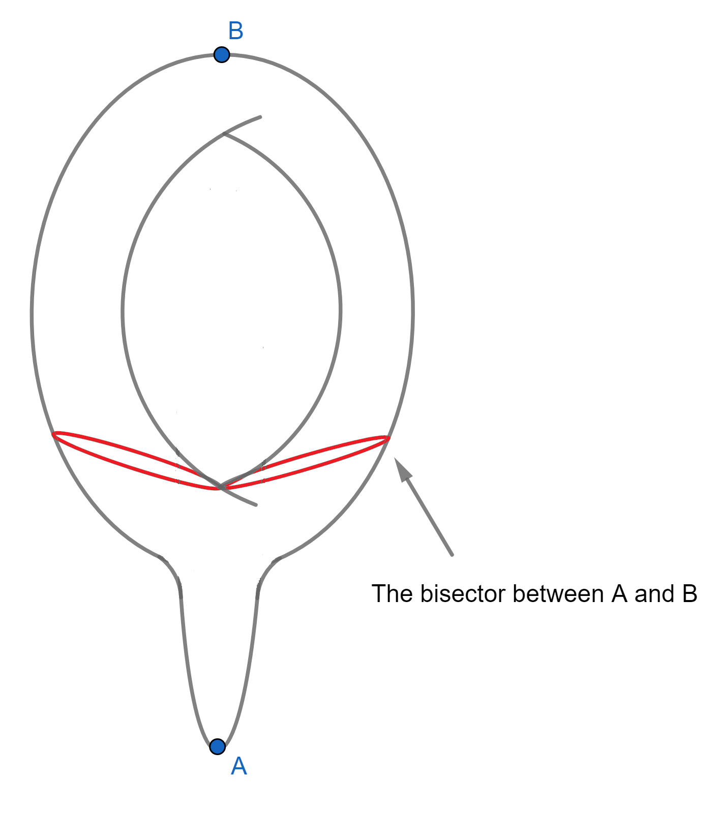
Figure 1. An example in which the bisector between two points is not a submanifold.

There are special cases when the bisector between any two points is a submanifold globally. In [5], the author proves that any bisector between two points is a totally geodesic submanifold if and only if the manifold has constant curvature. An obvious example of this case is the round sphere, where any bisector is a great hypersphere. Hence, on the round sphere, any Voronoi surface is a part of a great hypersphere.

In this work, we prove the following local regularity result for the bisectors on any manifold. In fact, we show that when two points are close enough, then an open neighborhood on the bisector around the midpoint of the minimizing geodesic connecting those two points is a $d-1$ dimensional submanifold. The proof of the proposition with a figure to illustrate the statement of the proposition is in Appendix B.

Proposition 3.2.

Suppose $\delta$ is small enough depending on the bounds of the sectional curvatures and the injectivity radius of $\mathcal{N}$. For any $\mathbf{y}_{i}\in\mathcal{N}$, let $B_{\delta}(\mathbf{y}_{i})$ be an open geodesic ball of radius $\delta$ at $\mathbf{y}_{i}$. Suppose $\mathbf{y}_{j}\in B_{\delta}(\mathbf{y}_{i})$ and $G_{ij}$ is the bisector between $\mathbf{y}_{i}$ and $\mathbf{y}_{j}$. Then, $M_{ij}=B_{\delta}(\mathbf{y}_{i})\cap G_{ij}$ is a $d-1$ dimensional submanifold. Let $\mathbf{y}^{*}$ be the midpoint of the minimizing geodesic between $\mathbf{y}_{i}$ and $\mathbf{y}_{j}$. Then $\mathbf{y}^{*}\in M_{ij}$ and the minimizing geodesic between $\mathbf{y}_{i}$ and $\mathbf{y}_{j}$ is perpendicular to $M_{ij}$ at $\mathbf{y}^{*}$.

Since $\{\mathbf{y}_{i}\}_{i=1}^{n}$ are sampled based on a density function $\rho^{**}$ with a positive lower bound, when $n$ is large enough, with high probability, there are enough points in a small geodesic ball. Hence, we can assume that each Voronoi cell is small enough so that it is contained in a geodesic ball. We propose the following assumption.

Assumption 3.3.

For $\delta$ defined in Proposition 3.2, let $B_{\frac{\delta}{2}}(\mathbf{y}_{i})$ be an open geodesic ball centered at $y_{i}$ with radius $\frac{\delta}{2}$. We assume that when $n$ is large enough, we have $C_{i}\subset B_{\frac{\delta}{2}}(\mathbf{y}_{i})$ for $i=1,\cdots,n$.

Suppose $\Gamma_{ij}$ is the Voronoi face between $\mathbf{y}_{i}$ and $\mathbf{y}_{j}$, Assumption 3.3 implies that $\mathbf{y}_{j}\in B_{\delta}(y_{i})$. Based on Assumption 3.3 and Proposition 3.2, the interior of the Voronoi face $\Gamma_{ij}$ is an open subset of a submanifold $M_{ij}$. Hence, there is a well defined unit outward normal vector field $\mathbf{n}$ on each $\partial C_{i}$ and we can apply the divergence Theorem on each Voronoi cell.

Recall the Fokker-Planck equation on $\mathcal{N}$ (3.1). We first recast (3.1) in the relative entropy form

(3.8) $$\partial_{t}\rho^{\mathcal{N}}_{t}=\text{div}_{\mathcal{N}}\left(\pi\nabla_{\mathcal{N}}\left(\frac{\rho^{\mathcal{N}}_{t}}{\pi}\right)\right).$$

We drop the dependence $t,\mathcal{N}$ in the short hand notation $\rho=\rho_{t}^{\mathcal{N}}$. We integrate this on $C_{i}$ and use the divergence theorem on cell $C_{i}$ to obtain

(3.9) $$\frac{\,\mathrm{d}}{\,\mathrm{d}t}\int_{C_{i}}\rho\mathcal{H}^{d}(C_{i})=\sum_{j\in\text{VF}(i)}\int_{\Gamma_{ij}}\pi\mathbf{n}\cdot\nabla_{\mathcal{N}}\left(\frac{\rho}{\pi}\right)\mathcal{H}^{d-1}(\Gamma_{ij}),$$

where $\mathbf{n}$ is the unit outward normal vector field on $\partial C_{i}$.

To design the numerical algorithm, first, let us clarify the probability on each cell. Then the probability in $C_{i}$ can be approximated as

(3.10) $$\int_{C_{i}}\rho(\mathbf{y})\mathcal{H}^{d}(C_{i})\approx\rho(\mathbf{y}_{i})(1+\operatorname{diam}(C_{i}))|C_{i}|.$$

Second, we use $\rho_{i}$ to approximate the exact solution $\rho(\mathbf{y}_{i})$ on each cell $C_{i}$. Let $\pi_{i}$ be the approximated equilibrium density at $\mathbf{y}_{i}$ satisfying $\sum_{i=1}^{n}\pi_{i}|C_{i}|=1$. Notice $\rho_{\infty}(\mathbf{y})\propto e^{-{U_{\mathcal{N}}(\mathbf{y})}}$, so $\pi_{i}>0$ for all $i$. Then the surface gradient in (3.9) can be approximated by

(3.11) $$\sum_{j\in\text{VF}(i)}\int_{\Gamma_{ij}}\pi\mathbf{n}\cdot\nabla_{\mathcal{N}}\left(\frac{\rho}{\pi}\right)\mathcal{H}^{d-1}(\Gamma_{ij})\approx\frac{1}{2}\sum_{j\in\text{VF}(i)}\frac{\pi_{i}+\pi_{j}}{|y_{i}-y_{j}|}|\Gamma_{ij}|\left(\frac{\rho_{j}}{\pi_{j}}-\frac{\rho_{i}}{\pi_{i}}\right).$$

Therefore, combining (3.10) and (3.11), we give the following finite volume scheme. For $i=1,\cdots,n$,

(3.12) $$\frac{\,\mathrm{d}}{\,\mathrm{d}t}\rho_{i}|C_{i}|=\frac{1}{2}\sum_{j\in\text{VF}(i)}\frac{\pi_{i}+\pi_{j}}{|y_{i}-y_{j}|}|\Gamma_{ij}|\left(\frac{\rho_{j}}{\pi_{j}}-\frac{\rho_{i}}{\pi_{i}}\right).$$

Let $\chi_{\scriptscriptstyle{C_{i}}}$ be the characteristic function such that $\chi_{\scriptscriptstyle{C_{i}}}=1$ for $\mathbf{y}\in C_{i}$ and $0$ otherwise. Then

$$\rho^{\text{approx}}(\mathbf{y}):=\sum_{i=1}^{n}\rho_{i}\chi_{\scriptscriptstyle{C_{i}}}(\mathbf{y})$$

is the piecewise constant probability distribution on $\mathcal{N}$ provided $\sum_{i=1}^{n}\rho_{i}|C_{i}|=1$ and $\rho_{i}\geq 0$. We will prove later in the convergence analysis Theorem 3.7 that the exact solution $\rho$ can be approximated by the numerical piecewise constant probability distribution constructed from $\rho_{i},i=1,\cdots,n$.

We will first formulate finite volume scheme (3.12) as the forward equation for a Markov process with basic properties such as ergodicity in Section 3.2. We then show the truncation error analysis and stability analysis and thus convergence of the scheme (3.12) later in Section 3.3.

3.2. Associated Markov process, detailed balance and ergodicity

We will first formulate finite volume scheme (3.12) as the forward equation for a Markov process and then in Proposition 3.5, we study the generator of the Markov process, which leads to ergodicity of $\frac{\rho_{i}(t)}{\pi_{i}}$. Roughly speaking, the forward equation leads to the conservation law while the backward equation leads to maximum norm estimates for $\frac{\rho_{i}}{\pi_{i}}$.

Lemma 3.4.

Let $\pi_{i}>0$ for all $i=1,\cdots,n$. The finite volume scheme (3.12) is the forward equation for a Markov Process with transition probability $P_{ji}$ (from state $j$ to $i$) and jump rate $\eta_{j}$

(3.13) $$\frac{\,\mathrm{d}}{\,\mathrm{d}t}\rho_{i}|C_{i}|=\Big{(}\sum_{j\in\text{VF}(i)}\eta_{j}P_{ji}\rho_{j}|C_{j}|\Big{)}-\eta_{i}\rho_{i}|C_{i}|,$$

where

(3.14) $$\eta_{i}=\sum_{j\neq i}Q_{ij}=:\frac{1}{2|C_{i}|\pi_{i}}\sum_{j\in\text{VF}(i)}\frac{\pi_{i}+\pi_{j}}{|y_{i}-y_{j}|}|\Gamma_{ij}|~{}{>0},\quad i=1,2,\cdots,n;$$

$$P_{ij}:=\left\{\begin{array}[]{cc}\displaystyle\frac{Q_{ij}}{\eta_{i}}=\frac{1}{\eta_{i}}\frac{\pi_{i}+\pi_{j}}{2\pi_{i}|C_{i}|}\frac{|\Gamma_{ij}|}{|y_{i}-y_{j}|},&j\in\text{VF}(i);\\ {}\hfil\\ \displaystyle 0,&j\notin\text{VF}(i).\end{array}\right.$$

1. $P$ is transition probability matrix satisfying $\sum_{j}P_{ij}=1$ and the detailed balance property

   (3.15) $$P_{ji}\eta_{j}\pi_{j}|C_{j}|=P_{ij}\eta_{i}\pi_{i}|C_{i}|=\frac{\pi_{i}+\pi_{j}}{2}\frac{|\Gamma_{ij}|}{|y_{i}-y_{j}|}\quad\forall i,\,j.$$

2. With $\{w_{i}\}_{i=1}^{n}:=\{\rho_{i}|C_{i}|\}_{i=1}^{n}$, we recast the forward equation (3.13) as

   (3.16) $$\frac{\,\mathrm{d}}{\,\mathrm{d}t}w=Q^{*}w,$$

   where $Q^{*}$ is the transpose of $Q$-matrix defined as

   (3.17) $$Q=(a_{ij})_{n\times n},\quad a_{ij}:=\left\{\begin{array}[]{cc}-\eta_{i},&j=i;\\ \eta_{i}P_{ij},&j\neq i.\end{array}\right.$$

3. $\sum_{i=j}^{n}a_{ij}=0$, which gives the conservation law for $\sum_{i}w_{i}$

   (3.18) $$\frac{\,\mathrm{d}}{\,\mathrm{d}t}\sum_{i=1}^{n}w_{i}=\sum_{i=1}^{n}\sum_{j=1}^{n}a_{ji}w_{j}=0;$$

4. We have the dissipation relation for $\chi^{2}$-divergence

   (3.19) $$\frac{\,\mathrm{d}}{\,\mathrm{d}t}\sum_{i}\frac{\rho^{2}_{i}}{\pi_{i}}|C_{i}|=-\sum_{i,j}\frac{\pi_{i}+\pi_{j}}{2}\frac{|\Gamma_{ij}|}{|y_{i}-y_{j}|}\left(\frac{\rho_{j}}{\pi_{j}}-\frac{\rho_{i}}{\pi_{i}}\right)^{2}.$$

Proof.

First, one can rewrite (3.12) as (3.13) with $\eta_{i}=\frac{1}{2|C_{i}|\pi_{i}}\sum_{j\in\text{VF}(i)}\frac{\pi_{i}+\pi_{j}}{|y_{i}-y_{j}|}|\Gamma_{ij}|$ and $P_{ji}\eta_{j}=\frac{\pi_{i}+\pi_{j}}{2|y_{i}-y_{j}|}\frac{|\Gamma_{ij}|}{\pi_{j}|C_{j}|}$. Then since $\frac{\pi_{i}+\pi_{j}}{|y_{i}-y_{j}|}|\Gamma_{ij}|$ is symmetric, we have

(3.20) $$\frac{\,\mathrm{d}}{\,\mathrm{d}t}(\sum_{i=1}^{n}|C_{i}|\rho_{i})=\sum_{i,j}\frac{1}{2}\frac{\pi_{i}+\pi_{j}}{|y_{i}-y_{j}|}|\Gamma_{ij}|\left(\frac{\rho_{j}}{\pi_{j}}-\frac{\rho_{i}}{\pi_{i}}\right)=0.$$

Second we can check

(3.21) $$\sum_{i}P_{ji}=\sum_{i\in\text{VF}(j)}P_{ji}=\frac{1}{\eta_{j}}\sum_{i\in\text{VF}(j)}\frac{\pi_{i}+\pi_{j}}{2|y_{i}-y_{j}|}\frac{|\Gamma_{ij}|}{\pi_{j}|C_{j}|}=1.$$

Third the detailed balance property comes from the symmetric property of $\frac{\pi_{i}+\pi_{j}}{|y_{i}-y_{j}|}|\Gamma_{ij}|$ and

(3.22) $$\eta_{j}P_{ji}\pi_{j}|C_{j}|=\frac{\pi_{i}+\pi_{j}}{2|y_{i}-y_{j}|}|\Gamma_{ij}|=\eta_{i}P_{ij}\pi_{i}|C_{i}|.$$

Next, the conservation law follows directly from $\sum_{i=1}^{n}a_{ji}=0$ by (3.17) and (3.21). Denote the diagonal rate matrix as ${R}=\text{diag}({\eta}_{j})$, then we obtain $Q$-matrix ${Q}={R}({P}-I)$.

Finally, by detailed balance property (3.15) and $\sum_{j}P_{ij}=1$, we recast (3.13) as

(3.23) $$\frac{\,\mathrm{d}}{\,\mathrm{d}t}\rho_{i}|C_{i}| =\sum_{j\in\text{VF}(i)}\eta_{i}P_{ij}\pi_{i}|C_{i}|\frac{\rho_{j}}{\pi_{j}}-\eta_{i}\pi_{i}|C_{i}|\frac{\rho_{i}}{\pi_{i}}$$

$$=\sum_{j\in\text{VF}(i)}\eta_{i}\pi_{i}|C_{i}|P_{ij}\left(\frac{\rho_{j}}{\pi_{j}}-\frac{\rho_{i}}{\pi_{i}}\right)=\sum_{j\in\text{VF}(i)}\frac{\pi_{i}+\pi_{j}}{2|y_{i}-y_{j}|}|\Gamma_{ij}|\left(\frac{\rho_{j}}{\pi_{j}}-\frac{\rho_{i}}{\pi_{i}}\right)$$

Multiplying this by $\frac{\rho_{i}}{\pi_{i}}$ and show that

(3.24) $$\frac{\,\mathrm{d}}{\,\mathrm{d}t}\sum_{i}\frac{\rho^{2}_{i}}{\pi_{i}}|C_{i}|=-\sum_{i,j}\frac{\pi_{i}+\pi_{j}}{2}\frac{|\Gamma_{ij}|}{|y_{i}-y_{j}|}\left(\frac{\rho_{j}}{\pi_{j}}-\frac{\rho_{i}}{\pi_{i}}\right)^{2}.$$

This gives the dissipation relation (3.19).

∎

Proposition 3.5.

Let $\pi_{i}>0$ for all $i=1,\cdots,n$. Let $Q:=(a_{ij})_{n\times n}$ be the $Q$-matrix defined in (3.17). Then $\{u_{i}\}_{i=1}^{n}:=\{\frac{\rho_{i}}{\pi_{i}}\}_{i=1}^{n}$ is the solution to the backward equation

(3.25) $$\frac{\,\mathrm{d}}{\,\mathrm{d}t}u=Qu.$$

Moreover, let $\eta_{i}$ be the jump rate defined in (3.14). We conclude $0$ is the simple, principle eigenvalue of $Q$ with the ground state $\{1,1,\cdots,1\}$. We thus have the exponential decay of $\rho_{i}(t)$ with respect to time $t$,

(3.26) $$\max_{i}\frac{|\rho_{i}(t)-\pi_{i}|}{\pi_{i}}\leq ce^{-(\lambda_{1}-|\lambda_{2}|)t},$$

where $\lambda_{1}>\max_{i}\eta_{i}$ is the principle eigenvalue of $\lambda I+Q$, $|\lambda_{2}|<\lambda_{1}$ is the second largest eigenvalue of $\lambda_{1}I+Q$, and $\lambda_{1}-|\lambda_{2}|>0$ is the spectral gap of $\lambda_{1}I+Q$.

Proof.

Recall (3.23). We recast the forward equation (3.13) as

(3.27) $$\frac{\,\mathrm{d}}{\,\mathrm{d}t}\rho_{i}|C_{i}|=\sum_{j\in\text{VF}(i)}\eta_{i}P_{ij}\pi_{i}|C_{i}|\frac{\rho_{j}}{\pi_{j}}-\eta_{i}\pi_{i}|C_{i}|\frac{\rho_{i}}{\pi_{i}},$$

which gives

(3.28) $$\frac{\,\mathrm{d}}{\,\mathrm{d}t}\frac{\rho_{i}}{\pi_{i}}=\sum_{j\in\text{VF}(i)}\eta_{i}P_{ij}\frac{\rho_{j}}{\pi_{j}}-\eta_{i}\frac{\rho_{i}}{\pi_{i}}.$$

Next, we show $\{u_{i}\}_{i=1}^{n}:=\{\frac{\rho_{i}}{\pi_{i}}\}_{i=1}^{n}$ is the solution to this backward equation. Recast (3.28) as

(3.29) $$\frac{\,\mathrm{d}}{\,\mathrm{d}t}u_{i}=\sum_{j=1}^{n}a_{ij}u_{j}.$$

Here $Q=\{a_{ij}\}$ is the generator of the backward equation

(3.30) $$\frac{\,\mathrm{d}}{\,\mathrm{d}t}u=Qu.$$

One can check $\sum_{j=1}^{n}a_{ij}=0,$ $a_{ij}\geq 0$ for $j\neq i$ and $a_{ii}<0.$

Moreover, due to the detailed balance property (3.15), we know $Q$ is self-adjoint in the weighted $l^{2}$-space

(3.31) $$\langle u,Qv\rangle_{\pi|C|}:=\sum_{i,j}u_{i}a_{ij}v_{j}\pi_{i}|C_{i}|=\sum_{i,j}a_{ji}u_{i}v_{j}\pi_{j}|C_{j}|=:\langle Qu,v\rangle_{\pi|C|}.$$

Thus we know the eigenvalues of $Q$ are real. For the matrix $\lambda_{1}I+Q$ with $\lambda_{1}>\max_{i}\eta_{i}$, we know each element is non-negative and $\lambda_{1}+\sum_{j=1}^{n}a_{ij}=\lambda_{1}>0$. Since the Voronoi tessellation $\mathcal{N}=\cup_{i=1}^{n}C_{i}$, when $\mathcal{N}$ is strongly connected, $\lambda_{1}I+Q$ is irreducible. By the Perron-Frobenius theorem for $\lambda_{1}I+Q$, we know the Perron–Frobenius eigenvalue (i.e. the principal eigenvalue) of $\lambda_{1}I+Q$ is $\lambda_{1}$ and $\lambda_{1}>0$ is a simple eigenvalue with the ground state $u^{*}:=(1,1,\cdots,1)$ and other eigenvalues $\lambda_{i}$ of $\lambda_{1}I+Q$ satisfy $|\lambda_{i}|<\lambda_{1}$. Therefore, we have

(3.32) $$\lambda_{1}(u-u^{*})+\frac{\,\mathrm{d}}{\,\mathrm{d}t}(u-u^{*})=(\lambda_{1}I+Q)(u-u^{*}).$$

Let $\|\cdot\|$ be the weighted $l^{2}$ norm defined as $\|v\|^{2}:=\sum_{i}v_{i}^{2}\pi_{i}|C_{i}|.$ Taking weighted inner product of (3.32) with $u-u^{*}$ and from $\langle u-u^{*},u^{*}\rangle_{\pi|C|}=0$, we have

(3.33) $$\lambda_{1}\|u-u^{*}\|^{2}+\frac{1}{2}\frac{\,\mathrm{d}}{\,\mathrm{d}t}(\|u-u^{*}\|^{2})=\langle(\lambda_{1}I+Q)(u-u^{*}),~{}u-u^{*}\rangle_{\pi|C|}\leq|\lambda_{2}|\|u-u^{*}\|^{2},$$

where we used $|\lambda_{2}|<\lambda_{1}$ is the second largest eigenvalue of $\lambda_{1}I+Q$. This gives

(3.34) $$\frac{\,\mathrm{d}}{\,\mathrm{d}t}\|u-u^{*}\|\leq(|\lambda_{2}|-\lambda_{1})\|u-u^{*}\|.$$

Therefore we obtain the exponential decay of $u$ to its ground state $u^{*}$

(3.35) $$\|u-u^{*}\|\leq ce^{(|\lambda_{2}|-\lambda_{1})t}.$$

Here $\lambda_{1}-|\lambda_{2}|>0$ is the spectral gap of $\lambda_{1}I+Q$. ∎

We refer to [39] for the ergodicity of finite volume schemes in an unbounded space. We refer to [42, 13, 44, 24, 25, 29] for more discussions on the corresponding generalized gradient flow of the relative entropy with graph Wasserstein distance on discrete space and Benamou-Brenier formula. See also [38, 57, 30] for some related data-driven algorithms when solving equations on a network graph and for irreversible processes.

3.3. Truncation error estimate, stability and convergence of the finite volume scheme (3.12)

In this section we prove the stability of (3.12) in Lemma 3.6. Then we obtain the convergence of the solution to finite volume scheme (3.12) to the solution of Fokker-Planck equation (3.1) in Theorem 3.7.

First, we have the following stability property, which corresponds to the Markov chain version of the Crandall-Tartar lemma for monotone schemes. This lemma is also known as the total variation diminishing for two density solutions.

Lemma 3.6.

Any two solutions $\rho_{i}$ and $\tilde{\rho}_{i}$ to finite volume scheme (3.13) have the following stability properties

(3.36) $$\frac{\,\mathrm{d}}{\,\mathrm{d}t}\sum_{i=1}^{n}\left|\rho_{i}-\tilde{\rho}_{i}|\right|C_{i}|\leq 0;$$

$$\frac{\,\mathrm{d}}{\,\mathrm{d}t}\sum_{i=1}^{n}\left|\dot{\rho}_{i}\right||C_{i}|\leq 0,$$

where $\dot{\rho}_{i}$ is the time derivative of $\rho_{i}(t)$.

Proof.

First assume $\rho_{i}$ and $\tilde{\rho}_{i}$ are two solutions to finite volume scheme (3.13). We have

(3.37) $$\frac{\,\mathrm{d}}{\,\mathrm{d}t}(\rho_{i}|C_{i}|-\tilde{\rho}_{i}|C_{i}|)=\sum_{j\in\text{VF}(i)}P_{ji}\eta_{j}|C_{j}|(\rho_{j}-\tilde{\rho}_{j})-\eta_{i}|C_{i}|(\rho_{i}-\tilde{\rho}_{i}).$$

Notice that for any function $u$, multiplying $u$ by its sign gives an absolute value $|u|$. From [34, Lemma 7.6], the derivative of $|u|$ equals the derivative of $u$ multiplied by the sign of $u$, i.e., $D|u|=\text{sgn}(u)Du.$Multiply $\text{sgn}(\rho_{i}-\tilde{\rho}_{i})$ to both sides and then take summation with respect to $i$

(3.38) $$\frac{\,\mathrm{d}}{\,\mathrm{d}t}\sum_{i=1}^{n}|C_{i}||\rho_{i}-\tilde{\rho}_{i}|\leq\sum_{i,j}P_{ji}\eta_{j}|C_{j}||\rho_{j}-\tilde{\rho}_{j}|-\sum_{i=1}^{n}\eta_{i}|C_{i}||\rho_{i}-\tilde{\rho}_{i}|=0,$$

where we used $\sum_{i\in\text{VF}(j)}P_{ji}=1$. Second, take time derivative in (3.13), then we have

(3.39) $$\frac{\,\mathrm{d}^{2}}{\,\mathrm{d}t^{2}}\rho_{i}|C_{i}|=\sum_{j\in\text{VF}(i)}P_{ji}\eta_{j}|C_{j}|\dot{\rho}_{j}-\eta_{i}|C_{i}|\dot{\rho}_{i}.$$

Then similarly we can multiply $\text{sgn}(\dot{\rho}_{i})$ to both sides and obtain

(3.40) $$\frac{\,\mathrm{d}}{\,\mathrm{d}t}\sum_{i=1}^{n}|C_{i}||\dot{\rho}_{i}|\leq\sum_{i,j}P_{ji}\eta_{j}|C_{j}||\dot{\rho}_{j}|-\sum_{i=1}^{n}\eta_{i}|C_{i}||\dot{\rho}_{i}|=0,$$

where we used $\sum_{i\in\text{VF}(j)}P_{ji}=1$. ∎

We conclude this section by the following convergence theorem in the weighted $L^{2}$ sense. Although the proof of the convergence theorem is rather standard, cf. [26], however the error estimation on manifold requires some careful treatments for the symmetric cancellation and some approximation lemmas for the Voronoi tessellation.

Theorem 3.7 (Convergence).

Suppose $\rho(\mathbf{y},t)$, $t\in[0,T]$ is a smooth solution to Fokker-Planck equation (3.1) on manifold $\mathcal{N}\subset\mathbb{R}^{\ell}$ with initial density $\rho^{0}(\mathbf{y})$. Let $\mathcal{N}=\cup_{i=1}^{n}C_{i}$ be the Voronoi tessellation of manifold $\mathcal{N}$ based on $\{\mathbf{y}_{i}\}_{i=1}^{n}$. Let

(3.41) $$h=\max\big{(}\max_{i=1,\ldots,n}(\operatorname{diam}(C_{i})),\max_{i=1,\ldots,n}(\max_{j\in\text{VF}(i)}d_{\mathcal{N}}(\mathbf{y}_{i},\mathbf{y}_{j}))\big{)}$$

Let $\{\rho_{i}\}_{i=1}^{n}$ be the solution to the finite volume scheme (3.12) with initial data $\{\rho_{i}^{0}\}_{i=1}^{n}$ and $e_{i}:=\rho(\mathbf{y}_{i})-\rho_{i}$. Under Assumption 3.3, we have the following error estimate

(3.42) $$\max_{t\in[0,T]}\sum_{i}e_{i}(t)^{2}\frac{|C_{i}|}{\pi_{i}}\leq\big{(}\sum_{i}e_{i}(0)^{2}\frac{|C_{i}|}{\pi_{i}}+O(h^{2}(nh\max_{i}|\partial C_{i}|+1))\big{)}e^{T},$$

where the constant in $O(h^{2}(nh\max_{i}|\partial C_{i}|+1))$ depends on $\operatorname{Vol}(\mathcal{N})$, the minimum of $\pi$, the $C^{1}$ norm of $\pi$, the $L^{\infty}$ norm of $\partial_{t}\nabla_{\mathcal{N}}\rho$ and the $C^{2}$ norm of $\frac{\rho}{\pi}$.

Proof.

Let $\rho_{i}^{e}:=\frac{1}{|C_{i}|}\int_{C_{i}}\rho\,\mathrm{d}y$ be the cell average. Plug the exact solution into the numerical scheme

(3.43) $$\partial_{t}(\rho_{i}^{e}|C_{i}|) =\sum_{j\in\text{VF}(i)}\frac{\pi_{i}+\pi_{j}}{2|\mathbf{y}_{i}-\mathbf{y}_{j}|}|\Gamma_{ij}|\left(\frac{\rho(\mathbf{y}_{j})}{\pi_{j}}-\frac{\rho(\mathbf{y}_{i})}{\pi_{i}}\right)+\sum_{j\in\text{VF}(i)}\varepsilon_{ij},$$

$$\varepsilon_{ij}:=\int_{\Gamma_{ij}}\pi\mathbf{n}_{ij}\cdot\nabla_{\mathcal{N}}\frac{\rho}{\pi}\,\mathrm{d}\mathcal{H}^{d-1}~{}-~{}\frac{\pi_{i}+\pi_{j}}{2|\mathbf{y}_{i}-\mathbf{y}_{j}|}|\Gamma_{ij}|\left(\frac{\rho(\mathbf{y}_{j})}{\pi_{j}}-\frac{\rho(\mathbf{y}_{i})}{\pi_{i}}\right),$$

where $\mathbf{n}_{ij}$ is the restriction of the unit outward normal vector field on $\Gamma_{ij}$. Exchanging $i,j$ above, we can see that $\varepsilon_{ij}$ is anti-symmetric.

Subtracting the numerical scheme (3.12) from (3.43), we have

(3.44) $$\frac{\,\mathrm{d}}{\,\mathrm{d}t}(e_{i}|C_{i}|)=\sum_{j\in\text{VF}(i)}\frac{\pi_{i}+\pi_{j}}{2|\mathbf{y}_{i}-\mathbf{y}_{j}|}|\Gamma_{ij}|\left(\frac{e_{j}}{\pi_{j}}-\frac{e_{i}}{\pi_{i}}\right)+\sum_{j\in\text{VF}(i)}\varepsilon_{ij}+\partial_{t}((\rho(\mathbf{y}_{i})-\rho_{i}^{e})|C_{i}|).$$

Similar to the dissipation relation (3.19), multiplying $\frac{e_{i}}{\pi_{i}}$ shows that

(3.45) $$\frac{\,\mathrm{d}}{\,\mathrm{d}t}\sum_{i}e_{i}^{2}\frac{|C_{i}|}{\pi_{i}}=-\sum_{i}\sum_{j\in\text{VF}(i)}\frac{\pi_{i}+\pi_{j}}{2|\mathbf{y}_{i}-\mathbf{y}_{j}|}|\Gamma_{ij}|\left(\frac{e_{j}}{\pi_{j}}-\frac{e_{i}}{\pi_{i}}\right)^{2}\,+\sum_{i}\sum_{j\in\text{VF}(i)}2\varepsilon_{ij}\frac{e_{i}}{\pi_{i}}+\sum_{i}2\partial_{t}(\rho(\mathbf{y}_{i})-\rho_{i}^{e})e_{i}\frac{|C_{i}|}{\pi_{i}}.$$

Since $\varepsilon_{ij}$ is anti-symmetric,

(3.46) $$\frac{\,\mathrm{d}}{\,\mathrm{d}t}\sum_{i}e_{i}^{2}\frac{|C_{i}|}{\pi_{i}} =-\sum_{i}\sum_{j\in\text{VF}(i)}\frac{\pi_{i}+\pi_{j}}{2|\mathbf{y}_{i}-\mathbf{y}_{j}|}|\Gamma_{ij}|\left(\frac{e_{j}}{\pi_{j}}-\frac{e_{i}}{\pi_{i}}\right)^{2}$$

$$\quad+\sum_{i}\sum_{j\in\text{VF}(i)}\varepsilon_{ij}\left(\frac{e_{i}}{\pi_{i}}-\frac{e_{j}}{\pi_{j}}\right)+\sum_{i}2\partial_{t}(\rho(\mathbf{y}_{i})-\rho_{i}^{e})e_{i}\frac{|C_{i}|}{\pi_{i}}.$$

Applying Young’s inequality to the last two terms, we have

(3.47) $$\sum_{i}\sum_{j\in\text{VF}(i)}\varepsilon_{ij}\left(\frac{e_{i}}{\pi_{i}}-\frac{e_{j}}{\pi_{j}}\right)$$

$$\leq\frac{1}{2}\sum_{i}\sum_{j\in\text{VF}(i)}\frac{\pi_{i}+\pi_{j}}{2|\mathbf{y}_{i}-\mathbf{y}_{j}|}|\Gamma_{ij}|\left(\frac{e_{j}}{\pi_{j}}-\frac{e_{i}}{\pi_{i}}\right)^{2}+\frac{1}{2}\sum_{i}\sum_{j\in\text{VF}(i)}\frac{\varepsilon^{2}_{ij}}{\frac{\pi_{i}+\pi_{j}}{2|\mathbf{y}_{i}-\mathbf{y}_{j}|}|\Gamma_{ij}|};$$

(3.48) $$\sum_{i}2\partial_{t}(\rho(\mathbf{y}_{i})-\rho_{i}^{e})e_{i}\frac{|C_{i}|}{\pi_{i}}\leq\sum_{i}[\partial_{t}(\rho(\mathbf{y}_{i})-\rho_{i}^{e})]^{2}\frac{|C_{i}|}{\pi_{i}}+\sum_{i}e_{i}^{2}\frac{|C_{i}|}{\pi_{i}}.$$

Thus we have

(3.49) $$\frac{\,\mathrm{d}}{\,\mathrm{d}t}\sum_{i}e_{i}^{2}\frac{|C_{i}|}{\pi_{i}}\leq -\frac{1}{2}\sum_{i}\sum_{j\in\text{VF}(i)}\frac{\pi_{i}+\pi_{j}}{2|\mathbf{y}_{i}-\mathbf{y}_{j}|}|\Gamma_{ij}|\left(\frac{e_{j}}{\pi_{j}}-\frac{e_{i}}{\pi_{i}}\right)^{2}+\frac{1}{2}\sum_{i}\sum_{j\in\text{VF}(i)}\frac{\varepsilon^{2}_{ij}}{\frac{\pi_{i}+\pi_{j}}{2|\mathbf{y}_{i}-\mathbf{y}_{j}|}|\Gamma_{ij}|}$$

$$+\sum_{i}[\partial_{t}(\rho(\mathbf{y}_{i})-\rho_{i}^{e})]^{2}\frac{|C_{i}|}{\pi_{i}}+\sum_{i}e_{i}^{2}\frac{|C_{i}|}{\pi_{i}}$$

$$\leq \sum_{i}\sum_{j\in\text{VF}(i)}\frac{\varepsilon^{2}_{ij}}{\frac{\pi_{i}+\pi_{j}}{2|\mathbf{y}_{i}-\mathbf{y}_{j}|}|\Gamma_{ij}|}+\sum_{i}[\partial_{t}(\rho(\mathbf{y}_{i})-\rho_{i}^{e})]^{2}\frac{|C_{i}|}{\pi_{i}}+\sum_{i}e_{i}^{2}\frac{|C_{i}|}{\pi_{i}}.$$

Next, we bound the term $\sum_{i}\sum_{j\in\text{VF}(i)}\frac{\varepsilon^{2}_{ij}}{\frac{\pi_{i}+\pi_{j}}{2|\mathbf{y}_{i}-\mathbf{y}_{j}|}|\Gamma_{ij}|}$.

Let $G_{ij}$ be the bisector between $\mathbf{y}_{i}$ and $\mathbf{y}_{j}$. Suppose $\mathbf{y}^{*}$ is the intersection point of the minimizing geodesic from $\mathbf{y}_{i}$ to $\mathbf{y}_{j}$ and $G_{ij}$. We have $d_{\mathcal{N}}(\mathbf{y}^{*},\mathbf{y}_{i})=d_{\mathcal{N}}(\mathbf{y}^{*},\mathbf{y}_{j})$. Suppose $T$ is the unit tangent vector of the minimizing geodesic at $\mathbf{y}^{*}$. From the Taylor expansion of $\frac{\rho}{\pi}$ along the geodesic, we have

(3.50) $$\frac{\rho}{\pi}(\mathbf{y}_{j})-\frac{\rho}{\pi}(\mathbf{y}^{*})=T\cdot\nabla_{\mathcal{N}}\frac{\rho}{\pi}(\mathbf{y}^{*})d_{\mathcal{N}}(\mathbf{y}^{*},\mathbf{y}_{j})+O(d^{2}_{\mathcal{N}}(\mathbf{y}^{*},\mathbf{y}_{j})),$$

(3.51) $$\frac{\rho}{\pi}(\mathbf{y}^{*})-\frac{\rho}{\pi}(\mathbf{y}_{i})=T\cdot\nabla_{\mathcal{N}}\frac{\rho}{\pi}(\mathbf{y}^{*})d_{\mathcal{N}}(\mathbf{y}^{*},\mathbf{y}_{i})+O(d^{2}_{\mathcal{N}}(\mathbf{y}^{*},\mathbf{y}_{i})).$$

By Assumption 3.3 and Proposition 3.2, $\mathbf{n}_{ij}$ can be extended to a unit normal vector field on the $d-1$ dimensional submanifold $M_{ij}\subset G_{ij}$. We also call the extension to be $\mathbf{n}_{ij}$. We have $T=\mathbf{n}_{ij}(\mathbf{y}^{*})$. Therefore, if we add the above two equations , we have

(3.52) $$\frac{\rho}{\pi}(\mathbf{y}_{j})-\frac{\rho}{\pi}(\mathbf{y}_{i})=\mathbf{n}_{ij}\cdot\nabla_{\mathcal{N}}\frac{\rho}{\pi}(\mathbf{y}^{*})d_{\mathcal{N}}(\mathbf{y}_{i},\mathbf{y}_{j})+O(d^{2}_{\mathcal{N}}(\mathbf{y}_{i},\mathbf{y}_{j})).$$

Hence,

(3.53) $$\mathbf{n}_{ij}\cdot\nabla_{\mathcal{N}}\frac{\rho}{\pi}(\mathbf{y}^{*})=\frac{\frac{\rho(\mathbf{y}_{j})}{\pi_{j}}-\frac{\rho(\mathbf{y}_{i})}{\pi_{i}}}{d_{\mathcal{N}}(\mathbf{y}_{i},\mathbf{y}_{j})}+O(d_{\mathcal{N}}(\mathbf{y}_{i},\mathbf{y}_{j}))=\frac{\frac{\rho(\mathbf{y}_{j})}{\pi_{j}}-\frac{\rho(\mathbf{y}_{i})}{\pi_{i}}}{|\mathbf{y}_{i}-\mathbf{y}_{j}|}+O(d_{\mathcal{N}}(\mathbf{y}_{i},\mathbf{y}_{j})),$$

where we apply Lemma 3.9 in the last step. Similarly,

(3.54) $$\pi(\mathbf{y}_{j})-\pi(\mathbf{y}^{*})=O(d_{\mathcal{N}}(\mathbf{y}^{*},\mathbf{y}_{j})),$$

(3.55) $$\pi(\mathbf{y}^{*})-\pi(\mathbf{y}_{i})=O(d_{\mathcal{N}}(\mathbf{y}^{*},\mathbf{y}_{i})).$$

Hence,

(3.56) $$\pi(\mathbf{y}^{*})=\frac{\pi_{i}+\pi_{j}}{2}+O(d_{\mathcal{N}}(\mathbf{y}_{i},\mathbf{y}_{j})).$$

Therefore,

(3.57) $$\pi(\mathbf{y}^{*})\mathbf{n}_{ij}\cdot\nabla_{\mathcal{N}}\frac{\rho}{\pi}(\mathbf{y}^{*})=\frac{\pi_{i}+\pi_{j}}{2}\frac{\frac{\rho(\mathbf{y}_{j})}{\pi_{j}}-\frac{\rho(\mathbf{y}_{i})}{\pi_{i}}}{|\mathbf{y}_{i}-\mathbf{y}_{j}|}+O(d_{\mathcal{N}}(\mathbf{y}_{i},\mathbf{y}_{j})).$$

For any $\mathbf{y}$ on $\Gamma_{ij}$,

(3.58) $$\pi(\mathbf{y})\mathbf{n}_{ij}\cdot\nabla_{\mathcal{N}}\frac{\rho}{\pi}(\mathbf{y})= \pi(\mathbf{y}^{*})\mathbf{n}\cdot\nabla_{\mathcal{N}}\frac{\rho}{\pi}(\mathbf{y}^{*})+O(d_{\mathcal{N}}(\mathbf{y},\mathbf{y}^{*}))$$

$$= \pi(\mathbf{y}^{*})\mathbf{n}\cdot\nabla_{\mathcal{N}}\frac{\rho}{\pi}(\mathbf{y}^{*})+O(d_{\mathcal{N}}(\mathbf{y}_{i},\mathbf{y})+d_{\mathcal{N}}(\mathbf{y}_{i},\mathbf{y}_{j}))$$

(3.59) $$= \pi(\mathbf{y}^{*})\mathbf{n}\cdot\nabla_{\mathcal{N}}\frac{\rho}{\pi}(\mathbf{y}^{*})+O(\operatorname{diam}(C_{i})+d_{\mathcal{N}}(\mathbf{y}_{i},\mathbf{y}_{j})),$$

where $\operatorname{diam}(C_{i})$ is the diameter of $C_{i}$ measured with respect to the distance in $\mathcal{N}$. Thus,

(3.60) $$\pi(\mathbf{y})\mathbf{n}_{ij}\cdot\nabla_{\mathcal{N}}\frac{\rho}{\pi}(\mathbf{y})=\frac{\pi_{i}+\pi_{j}}{2}\frac{\frac{\rho(\mathbf{y}_{j})}{\pi_{j}}-\frac{\rho(\mathbf{y}_{i})}{\pi_{i}}}{|\mathbf{y}_{i}-\mathbf{y}_{j}|}+O(\operatorname{diam}(C_{i})+d_{\mathcal{N}}(\mathbf{y}_{i},\mathbf{y}_{j})).$$

We conclude that

(3.61) $${\varepsilon_{ij}}=O((\operatorname{diam}(C_{i})+d_{\mathcal{N}}(\mathbf{y}_{i},\mathbf{y}_{j}))|\Gamma_{ij}|).$$

Therefore,

(3.62) $$\frac{\varepsilon^{2}_{ij}}{\frac{\pi_{i}+\pi_{j}}{2|\mathbf{y}_{i}-\mathbf{y}_{j}|}|\Gamma_{ij}|}=O(d_{\mathcal{N}}(\mathbf{y}_{i},\mathbf{y}_{j})(\operatorname{diam}(C_{i})+d_{\mathcal{N}}(\mathbf{y}_{i},\mathbf{y}_{j}))^{2}|\Gamma_{ij}|).$$

If we sum up all $j\in\text{VF}(i)$,

(3.63) $$\sum_{j\in\text{VF}(i)}\frac{\varepsilon^{2}_{ij}}{\frac{\pi_{i}+\pi_{j}}{2|\mathbf{y}_{i}-\mathbf{y}_{j}|}|\Gamma_{ij}|}=\max_{j\in\text{VF}(i)}d_{\mathcal{N}}(\mathbf{y}_{i},\mathbf{y}_{j})(\operatorname{diam}(C_{i})+d_{\mathcal{N}}(\mathbf{y}_{i},\mathbf{y}_{j}))^{2}O(|\partial C_{i}|).$$

Hence,

(3.64) $$\sum_{i}\sum_{j\in\text{VF}(i)}\frac{\varepsilon^{2}_{ij}}{\frac{\pi_{i}+\pi_{j}}{2|\mathbf{y}_{i}-\mathbf{y}_{j}|}|\Gamma_{ij}|}=O(nh^{3}\max_{i}|\partial C_{i}|),$$

where the constant depends on the minimum of $\pi$, the $C^{1}$ norm of $\pi$ and the $C^{2}$ norm of $\frac{\rho}{\pi}$.

Next, we bound $\sum_{i}[\partial_{t}(\rho(\mathbf{y}_{i})-\rho_{i}^{e})]^{2}\frac{|C_{i}|}{\pi_{i}}$

(3.65) $$\partial_{t}(\rho(\mathbf{y}_{i})-\rho_{i}^{e})=O(\operatorname{diam}(C_{i}))=O(h),$$

where the constant depends on the $L^{\infty}$ norm of $\partial_{t}\nabla_{\mathcal{N}}\rho$. Since $\sum_{i}|C_{i}|=\operatorname{Vol}(\mathcal{N})$,

(3.66) $$\sum_{i}[\partial_{t}(\rho(\mathbf{y}_{i})-\rho_{i}^{e})]^{2}\frac{|C_{i}|}{\pi_{i}}=O(h^{2}),$$

where the constant depends on the $L^{\infty}$ norm of $\partial_{t}\nabla_{\mathcal{N}}\rho$, $\operatorname{Vol}(\mathcal{N})$ and minimum of $\pi$. Hence ,

(3.67) $$\frac{\,\mathrm{d}}{\,\mathrm{d}t}\sum_{i}e_{i}^{2}\frac{|C_{i}|}{\pi_{i}}\leq O(h^{2}(nh\max_{i}|\partial C_{i}|+1))+\sum_{i}e_{i}^{2}\frac{|C_{i}|}{\pi_{i}}.$$

In conclusion,

(3.68) $$\max_{t\in[0,T]}\sum_{i}e_{i}(t)^{2}\frac{|C_{i}|}{\pi_{i}}\leq\big{(}\sum_{i}e_{i}(0)^{2}\frac{|C_{i}|}{\pi_{i}}+O(h^{2}(nh\max_{i}|\partial C_{i}|+1))\big{)}e^{T}.$$

∎

3.4. Approximation of Voronoi cells on manifold

Recall that $\{\mathbf{y}_{i}\}_{i=1}^{n}$ are samples on the smooth closed submanifold $\mathcal{N}$ in $\mathbb{R}^{\ell}$ based on the density function $\rho^{**}$. In this section, we introduce an algorithm to approximate the volumes of the Voronoi cells and the areas of the Voronoi faces constructed from $\{\mathbf{y}_{i}\}_{i=1}^{n}$.

First, we need the following definition.

Definition 3.8.

For any $0<r<1$ and $\mathbf{y}_{k}\in\{\mathbf{y}_{i}\}_{i=1}^{n}$, suppose $B^{\mathbb{R}^{\ell}}_{\sqrt{r}}(\mathbf{y}_{k})\cap\{\mathbf{y}_{i}\}_{i=1}^{n}=\{\mathbf{y}_{k,1},\cdots,\mathbf{y}_{k,\bar{N}_{k}}\}$. We define the discrete local covariance matrix at $\mathbf{y}_{k}$,

(3.69) $$C_{n,r}(\mathbf{y}_{k}):=\frac{1}{n}\sum_{i=1}^{\bar{N}_{k}}(\mathbf{y}_{k,i}-\mathbf{y}_{k})(\mathbf{y}_{k,i}-\mathbf{y}_{k})^{\top}\in\mathbb{R}^{\ell\times\ell}.$$

Suppose $\{\beta_{n,r,1},\cdots,\beta_{n,r,d}\}$ are the first $d$ orthonormal eigenvectors corresponding to $C_{n,r}(\mathbf{y}_{k})$’s largest $d$ eigenvalues. Define a map $\iota_{k}(u):\mathbb{R}^{\ell}\rightarrow\mathbb{R}^{d}$ as

(3.70) $$\iota_{k}(u):=(u^{\top}\beta_{n,r,1},\cdots,u^{\top}\beta_{n,r,d}).$$

For any $\mathbf{y}\in\mathbb{R}^{\ell}$, define $\tilde{\iota}_{k}(\mathbf{y})=\iota_{k}(\mathbf{y}-\mathbf{y}_{k})$.

Based on the above definition, we propose the following algorithm to find the approximated volumes $|\tilde{C}_{k}|$ of the Voronoi cells $C_{k}$ and the approximated areas $|\tilde{\Gamma}_{k\ell}|$ of the Voronoi faces $\Gamma_{k\ell}$.

Parameters : Algorithm inputs are the bandwidth $r$ and the threshold $s$

1

2Choose $0<r<1$. For each $\mathbf{y}_{k}\in\{\mathbf{y}_{i}\}_{i=1}^{n}$, find

$$B^{\mathbb{R}^{\ell}}_{\sqrt{r}}(\mathbf{y}_{k})\cap\{\mathbf{y}_{i}\}_{i=1}^{n}=:\{\mathbf{y}_{k,1},\cdots,\mathbf{y}_{k,\bar{N}_{k}}\},\quad B^{\mathbb{R}^{\ell}}_{r}(\mathbf{y}_{k})\cap\{\mathbf{y}_{i}\}_{i=1}^{n}=:\{\mathbf{y}_{k,1},\cdots,\mathbf{y}_{k,N_{k}}\}.$$

3Construct the matrix $C_{n,r}(\mathbf{y}_{k})$ as in (3.69) by using the $\{\mathbf{y}_{k,1},\cdots,\mathbf{y}_{k,\bar{N}_{k}}\}$. Find the orthonormal eigenvectors corresponding to $C_{n,r}(\mathbf{y}_{k})$’s largest $d$ eigenvalues. Denote them as $\{\beta_{n,r,1},\cdots,\beta_{n,r,d}\}$.

4Use $\{\beta_{n,r,1},\cdots,\beta_{n,r,d}\}$ to construct $\tilde{\iota}_{k}$ as in (3.70). Find $v_{k,i}=\tilde{\iota}_{k}(\mathbf{y}_{k,i})$, for $i=1,\cdots,N_{k}$.

5Find the Voronoi cell decomposition of $\{0,v_{k,1},\cdots,v_{k,N_{k}}\}$ in $\mathbb{R}^{d}$. Denote the Voronoi cell containing $0$ to be $\tilde{C}_{k,0}$ and the Voronoi cell containing $v_{k,i}$ to be $\tilde{C}_{k,i}$. Denote the face $\tilde{F}_{k,i}=\tilde{C}_{k,0}\cup\tilde{C}_{k,i}$.

6Find the approximation of $|C_{k}|$ as

(3.71) $$|\tilde{C}_{k}|:=|\tilde{C}_{k,0}|:=\mathcal{H}^{d}(\tilde{C}_{k,0}).$$

7Find $|\tilde{F}_{k,i}|=\mathcal{H}^{d-1}(\tilde{F}_{k,i})$. Define $\tilde{\Gamma}\in\mathbb{R}^{n\times n}$ such that

(3.74) $$A_{k\ell}:=\frac{\tilde{A}_{k\ell}+\tilde{A}_{\ell k}}{2},\quad\tilde{A}_{k\ell}=\left\{\begin{array}[]{ll}|\tilde{F}_{k,i}|&\mbox{if $\mathbf{y}_{\ell}=\mathbf{y}_{k,i}\in B^{\mathbb{R}^{\ell}}_{r}(\mathbf{y}_{k})$ ;}\\ 0&\mbox{otherwise}.\end{array}\right.$$

If $A_{k\ell}\geq s$, then $|\tilde{\Gamma}_{k\ell}|=A_{k\ell}$. Otherwise $|\tilde{\Gamma}_{k\ell}|=s$. Then $|\tilde{\Gamma}_{k\ell}|$ is an approximation of $|\Gamma_{k\ell}|$.

Algorithm 1 Approximation of the Voronoi cell

The idea of the above algorithm can be summarized as follows. For each $\mathbf{y}_{k}$, by using the points in a larger ball $B^{\mathbb{R}^{\ell}}_{\sqrt{r}}(\mathbf{y}_{k})$, we construct the matrix $C_{n,r}(\mathbf{y}_{k})$. Then, the first $d$ orthonormal eigenvectors will be an approximation of an orthonormal basis of $T_{\mathbf{y}_{k}}\mathcal{N}$. Next, we project the points in a smaller ball $B^{\mathbb{R}^{\ell}}_{r}(\mathbf{y}_{k})$ onto this tangent space approximation. Now the points around $\mathbf{y}_{k}$ are projected into a $d$ dimensional Euclidean space and $\mathbf{y}_{k}$ is projected to the origin. If we find the Voronoi cell around the origin in the Euclidean space, then it gives the approximation of the Voronoi cell around $\mathbf{y}_{k}$ in $\mathcal{N}$. Obviously, the better estimation of the tangent space we have, there are smaller errors in the approximation of the volumes of the Voronoi cells and the areas of the Voronoi faces.

Next, we provide a justification of the above algorithm. When the geodesic distance between two points on $\mathcal{N}$ is small, the next lemma relates the Euclidean distance and the geodesic distance between them. The proof can be found in Lemma B.3 in [56].

Lemma 3.9.

Suppose $\mathbf{y},\mathbf{y}^{\prime}\in\mathcal{N}$ such that $d_{\mathcal{N}}(y,y^{\prime})$ is small enough. Then

(3.75) $$\|\mathbf{y}^{\prime}-\mathbf{y}\|_{\mathbb{R}^{\ell}}=d_{\mathcal{N}}(\mathbf{y},\mathbf{y}^{\prime})(1+O(d^{2}_{\mathcal{N}}(\mathbf{y},\mathbf{y}^{\prime}))),$$

where the constant in $O(d^{2}_{\mathcal{N}}(\mathbf{y},\mathbf{y}^{\prime}))$ depending on the second fundamental form of $\mathcal{N}$ in $\mathbb{R}^{\ell}$ at $\mathbf{y}$.

The above lemma implies that if $r$ is small enough, then for all $\mathbf{y}_{k}$ and any $\mathbf{y}\in B^{\mathbb{R}^{\ell}}_{r}(\mathbf{y}_{k})\cap\mathcal{N}$, there is a constant $D_{1}>1$ depending on the second fundamental form of $\mathcal{N}$ in $\mathbb{R}^{\ell}$, such that

(3.76) $$d_{\mathcal{N}}(\mathbf{y},\mathbf{y}_{k})\leq D_{1}\|\mathbf{y}_{k}-\mathbf{y}\|_{\mathbb{R}^{\ell}}.$$

We further make the following assumption about the Voronoi cells and the distribution of $\{\mathbf{y}_{i}\}_{i=1}^{n}$ on $\mathcal{N}$.

Assumption 3.10.

For $n$ large enough, there exists $r$ depending on $n$ such that $nr^{d}$ is bounded from above and has a positive lower bound for all $n$ and $\frac{nr^{\frac{d}{2}}}{\log n}\rightarrow\infty$ as $n\rightarrow\infty$. Moreover, when $n$ is large enough, the following conditions about $r$ hold for any $\mathbf{y}_{k}$:

1. Suppose $B^{\mathbb{R}^{\ell}}_{r}(\mathbf{y}_{k})\cap\{\mathbf{y}_{i}\}_{i=1}^{n}=\{\mathbf{y}_{k,1},\cdots,\mathbf{y}_{k,N_{k}}\}$. We have $C_{k}\subset B^{\mathbb{R}^{\ell}}_{r}(\mathbf{y}_{k})$. Moreover, if $\Gamma_{kj}$ is a Voronoi surface of $C_{k}$ between $\mathbf{y}_{k}$ and $\mathbf{y}_{j}$, then $\mathbf{y}_{j}\in B^{\mathbb{R}^{\ell}}_{r}(\mathbf{y}_{k})$. Suppose $\mathbf{y}_{j}=\mathbf{y}_{k,m}$, then we introduce the notation $\Gamma_{k,m}=\Gamma_{kj}$.

2. For any $i=1,\cdots N_{k}$, there is a constant $D_{2}<1$ such that $d_{\mathcal{N}}(\mathbf{y}_{k,i},\mathbf{y}_{k})\geq D_{2}r$.

Next, we intuitively explain the relation between Assumption 3.10 and Algorithm 1. Recall that $\{\mathbf{y}_{i}\}_{i=1}^{n}$ are sampled based on a density function $\rho^{**}$ with a positive lower bound and upper bound. In Algorithm 1, we use the points in a larger ball $B^{\mathbb{R}^{\ell}}_{\sqrt{r}}(\mathbf{y}_{k})$ to approximate the tangent space $T_{\mathbf{y}_{k}}\mathcal{N}$. Since $\rho^{**}$ has a positive lower bound, the condition $\frac{nr^{\frac{d}{2}}}{\log n}\rightarrow\infty$ as $n\rightarrow\infty$ implies that the number of points in $B^{\mathbb{R}^{\ell}}_{\sqrt{r}}(\mathbf{y}_{k})$ goes to infinity as $n$ goes to infinity. Hence, we can have a good estimation of the tangent space. The condition that $nr^{d}$ is bounded from above and has a positive lower bound for all $n$ implies $r\rightarrow 0$ as $n\rightarrow\infty$. Since $\rho^{**}$ has an upper bound and a positive lower bound, it also implies that we will have enough but not too many points in the smaller ball $B^{\mathbb{R}^{\ell}}_{r}(\mathbf{y}_{k})$. Hence, (1) and (2) become mild assumption with this relation between $r$ and $n$. In fact, since $r\rightarrow 0$ as $n\rightarrow\infty$, (1) says that the Voronoi cell is in a small ball $B^{\mathbb{R}^{\ell}}_{r}(\mathbf{y}_{k})$. In (2), since there are not too many points in $B^{\mathbb{R}^{\ell}}_{r}(\mathbf{y}_{k})$, it is reasonable to assume the distance between the points in $B^{\mathbb{R}^{\ell}}_{r}(\mathbf{y}_{k})$ and $\mathbf{y}_{k}$ has a lower bound $D_{2}r$. With (1) and (2), we can show that the approximation to Voronoi cell in the tangent space is accurate enough for our analysis.

Consider the geodesic ball $B_{\frac{\delta}{2}}(y_{k})$ in Assumption 3.3. By Lemma 3.9, when $r$ is small enough, we have $B^{\mathbb{R}^{\ell}}_{r}(\mathbf{y}_{k})\cap\mathcal{N}\subset B_{\frac{\delta}{2}}(y_{i})$. Since $r\rightarrow 0$ as $n\rightarrow\infty$, we know that when $n$ is large enough, (1) in Assumption 3.10 implies Assumption 3.3. Hence, when $n$ is large enough, Assumption 3.10 with Proposition 3.2 implies that the interior of each Voronoi face of $C_{k}$ is an open subset of a $d-1$ dimensional submanifold.

The following lemma is a consequence of (2) in Assumption 3.10.

Lemma 3.11.

Under Assumption 3.10, $d_{\mathcal{N}}(\partial C_{k},y_{k})\geq\frac{1}{2}D_{2}r$. There are constants $K_{1}$ and $K_{2}$ depending on $D_{1}$, $D_{2}$ and the Ricci curvature of $\mathcal{N}$, such that

(3.77) $$K_{1}r^{d}\leq|C_{k}|\leq K_{2}r^{d},$$

Proof.

Suppose $G_{k,i}$ is the bisector between $\mathbf{y}_{k}$ and $\mathbf{y}_{k,i}$. Then $d_{\mathcal{N}}(\Gamma_{k,i},y_{k})\geq d_{\mathcal{N}}(G_{k,i},y_{k})\geq\frac{1}{2}D_{2}r$. Hence, $d_{\mathcal{N}}(\partial C_{k},y_{k})\geq\frac{1}{2}D_{2}r$. Therefore, each $C_{i}$ contains a geodesic ball of radius $\frac{1}{2}D_{2}r$ and is contained in the geodesic ball of radius $D_{1}r$. By Lemma B.1 in [56] when $r$ is small enough, the volume of a geodesic ball of radius $r$ can be bounded from below by $K^{\prime}_{1}r^{d}$ and from above by $K^{\prime}_{2}r^{d}$ where $K^{\prime}_{1}$ and $K^{\prime}_{2}$ depend on the Ricci curvature of $\mathcal{N}$. The conclusion follows. ∎

In the next proposition, we show that $|\tilde{C}_{k}|$ is a good approximation of $|C_{k}|$. The proof of the proposition is in the Appendix.

Proposition 3.12.

Let $|\tilde{C}_{k}|$ be the approximated volume of $C_{k}$ in (3.71). If $n$ is large enough, for $r$ satisfying Assumption 3.10, with probability greater than $1-\frac{1}{n^{2}}$, for all $\mathbf{y}_{k}$, we have $|\tilde{C}_{k}|=|\tilde{C}_{k,0}|=|C_{k}|(1+O(r))$.

Since we are approximating the tangent plane of the manifold $\mathcal{N}$, the error between $|\Gamma_{ki}|$ and $|\tilde{\Gamma}_{ki}|$ will not be much smaller than $|\Gamma_{ki}|$ itself when $|\Gamma_{ki}|$ is too small. However, in the next proposition, we show that if $|\Gamma_{ki}|$ is large enough, then $|\tilde{\Gamma}_{ki}|$ is a good approximation of $|\Gamma_{ki}|$. The proof of the proposition is in the appendix.

Proposition 3.13.

Let $|\tilde{\Gamma}_{ki}|$ be the approximated area of $\Gamma_{ki}$ in (3.74). If $n$ is large enough, for $r$ satisfying Assumption 3.10, let $s=a_{1}r^{d}$ in the last step of Algorithm 1 for some constant $a_{1}$, with probability greater than $1-\frac{1}{n^{2}}$, for all $\mathbf{y}_{k}$, we have

(3.78) $$|\Gamma_{ki}|=|\tilde{\Gamma}_{ki}|+O(r^{d}).$$

Hence, if $|\Gamma_{ki}|\geq a_{2}r^{d-1}$ for some constant $a_{2}$, then

(3.79) $$|\Gamma_{ki}|=|\tilde{\Gamma}_{ki}|(1+O(r))$$

At last, if we use our approximation of the volumes of the Voronoi cells and the areas of the Voronoi faces in (3.12) we have the following implementable finite volume scheme based only on the collected dataset $\{\mathbf{y}_{i}\}\subset\mathcal{N}$

(3.80) $$\frac{\,\mathrm{d}}{\,\mathrm{d}t}\tilde{\rho}_{i}|\tilde{C}_{i}|=\frac{1}{2}\sum_{j\in\text{VF}(i)}\frac{\pi_{i}+\pi_{j}}{|y_{i}-y_{j}|}|\tilde{\Gamma}_{ij}|\left(\frac{\tilde{\rho}_{j}}{\pi_{j}}-\frac{\tilde{\rho}_{i}}{\pi_{i}}\right).$$

Moreover, same as Lemma 3.4, we know the finite volume scheme (3.80) is the forward equation for a Markov Process with transition probability $\tilde{P}_{ji}$ and jump rate $\tilde{\eta}_{i}$

(3.81) $$\frac{\,\mathrm{d}}{\,\mathrm{d}t}\tilde{\rho}_{i}|\tilde{C}_{i}|=\sum_{j\in\text{VF}(i)}\tilde{\eta}_{j}\tilde{P}_{ji}\tilde{\rho}_{j}|\tilde{C}_{j}|-\tilde{\eta}_{i}\tilde{\rho}_{i}|\tilde{C}_{i}|,$$

where for $i=1,\cdots,n,\,j=1,\cdots,n$,

(3.82) $$\tilde{\eta}_{i}:=\frac{1}{2|\tilde{C}_{i}|\pi_{i}}\sum_{j\in\text{VF}(i)}\frac{\pi_{i}+\pi_{j}}{|y_{i}-y_{j}|}|\tilde{\Gamma}_{ij}|,$$

$$\tilde{P}_{ji}:=\frac{1}{\tilde{\eta}_{j}}\frac{\pi_{i}+\pi_{j}}{2\pi_{j}|\tilde{C}_{j}|}\frac{|\tilde{\Gamma}_{ij}|}{|y_{i}-y_{j}|},\quad j\in\text{VF}(i);\quad\tilde{P}_{ji}=0,\quad j\notin\text{VF}(i).$$

Similar to Lemma 3.4, we know $\tilde{P}$ is the transition probability matrix with row sum $1$. Denote the diagonal rate matrix as $\tilde{R}=\text{diag}(\tilde{\eta}_{j})$, then we also obtain an approximated $Q$-matrix $\tilde{Q}=\tilde{R}(\tilde{P}-I)$. Notice $\pi_{i}>0$ for all $i=1,\cdots,n$, so we always have $\tilde{\eta}_{i}>0$ for all $i$. It also satisfies the detailed balance property

(3.83) $$\tilde{\eta}_{j}\tilde{P}_{ji}\pi_{j}|\tilde{C}_{j}|=\tilde{\eta}_{i}\tilde{P}_{ij}\pi_{i}|\tilde{C}_{i}|,$$

conservation laws and the stability analysis in Lemma 3.6.

Now we state and prove the convergence of the implementable finite volume scheme (3.80). The bound of the error in the weighted $\ell^{2}$ norm is summarized in the following theorem. Due to the estimation error in the Voronoi cells and faces, the error in Theorem 3.7 $e^{T}$ is replaced by $e^{2T}$. Assume for $i=1,\cdots,n$, $|\text{VF}(i)|$, the cardinality of $\text{VF}(i)$, is order $1$.

Theorem 3.14.

Suppose $\rho(\mathbf{y},t)$, $t\in[0,T]$ is a smooth solution to the Fokker-Planck equation (3.1) on manifold $\mathcal{N}\subset\mathbb{R}^{\ell}$ with initial density $\rho^{0}(\mathbf{y})$. Let $\{\tilde{\rho}_{i}(t)\}_{i=1}^{n}$ be the solution of the finite volume scheme (3.80). Let $\tilde{e}_{i}:=\rho(\mathbf{y}_{i})-\tilde{\rho}_{i}$. If $n$ is large enough, for $r$ satisfying Assumption 3.10, we choose threshold $s=a_{1}r^{d}$ for some constant $a_{1}$ in Algorithm (1), with probability greater than $1-\frac{1}{n^{2}}$, we have

(3.84) $$\max_{t\in[0,T]}\sum_{i}\tilde{e}_{i}(t)^{2}\frac{|C_{i}|}{\pi_{i}}\leq\big{(}\sum_{i}\tilde{e}_{i}(0)^{2}\frac{|C_{i}|}{\pi_{i}}+cr\big{)}e^{2T},$$

where $c$ is a constant independent of $r$ and $n$.

Proof.

Define $\rho_{i}^{e}:=\frac{1}{|C_{i}|}\int_{C_{i}}\rho\,\mathrm{d}y$. Plug the exact solution into the numerical scheme

(3.85) $$\partial_{t}(\rho_{i}^{e}|C_{i}|)= \sum_{j\in\text{VF}(i)}\frac{\pi_{i}+\pi_{j}}{2|\mathbf{y}_{i}-\mathbf{y}_{j}|}|\tilde{\Gamma}_{ij}|\left(\frac{\rho(\mathbf{y}_{j})}{\pi_{j}}-\frac{\rho(\mathbf{y}_{i})}{\pi_{i}}\right)$$

$$+ \sum_{j\in\text{VF}(i)}\int_{{\Gamma}_{ij}}\pi\mathbf{n}_{ij}\cdot\nabla_{\mathcal{N}}\frac{\rho}{\pi}\,\mathrm{d}\mathcal{H}^{d-1}~{}-\sum_{j\in\text{VF}(i)}~{}\frac{\pi_{i}+\pi_{j}}{2|\mathbf{y}_{i}-\mathbf{y}_{j}|}|\tilde{\Gamma}_{ij}|\left(\frac{\rho(\mathbf{y}_{j})}{\pi_{j}}-\frac{\rho(\mathbf{y}_{i})}{\pi_{i}}\right),$$

where $\mathbf{n}_{ij}$ is the restriction of the unit outward normal vector field on $\Gamma_{ij}$. Subtracting the numerical scheme (3.80) from (3.85), we have

(3.86) $$\frac{\,\mathrm{d}}{\,\mathrm{d}t}\tilde{e}_{i}|C_{i}|= \sum_{j\in\text{VF}(i)}\frac{\pi_{i}+\pi_{j}}{2|y_{i}-y_{j}|}|{\tilde{\Gamma}}_{ij}|\left(\frac{\tilde{e}_{j}}{\pi_{j}}-\frac{\tilde{e}_{i}}{\pi_{i}}\right)+\sum_{j\in\text{VF}(i)}\varepsilon_{ij}+\partial_{t}((\rho(\mathbf{y}_{i})-\rho_{i}^{e})|C_{i}|)+\frac{\,\mathrm{d}}{\,\mathrm{d}t}\tilde{\rho}_{i}(|\tilde{C}_{i}|-|C_{i}|),$$

where

(3.87) $$\varepsilon_{ij}:=\int_{\Gamma_{ij}}\pi\mathbf{n}_{ij}\cdot\nabla_{\mathcal{N}}\frac{\rho}{\pi}\,\mathrm{d}\mathcal{H}^{d-1}~{}- ~{}\frac{\pi_{i}+\pi_{j}}{2|\mathbf{y}_{i}-\mathbf{y}_{j}|}|\Gamma_{ij}|\left(\frac{\rho(\mathbf{y}_{j})}{\pi_{j}}-\frac{\rho(\mathbf{y}_{i})}{\pi_{i}}\right)$$

$$+\frac{\pi_{i}+\pi_{j}}{2|y_{i}-y_{j}|}(|{\Gamma}_{ij}|-|{\tilde{\Gamma}}_{ij}|)\left(\frac{\rho(\mathbf{y}_{j})}{\pi_{j}}-\frac{\rho(\mathbf{y}_{i})}{\pi_{i}}\right)$$

Note that $\varepsilon_{ij}$ is anti-symmetric, hence by the same argument in Theorem 3.7, we have

(3.88) $$\frac{\,\mathrm{d}}{\,\mathrm{d}t}\sum_{i}\tilde{e}_{i}^{2}\frac{|C_{i}|}{\pi_{i}}\leq -\frac{1}{2}\sum_{i}\sum_{j\in\text{VF}(i)}\frac{\pi_{i}+\pi_{j}}{2|y_{i}-y_{j}|}|{\tilde{\Gamma}}_{ij}|\left(\frac{\tilde{e}_{j}}{\pi_{j}}-\frac{\tilde{e}_{i}}{\pi_{i}}\right)^{2}+\frac{1}{2}\sum_{i}\sum_{j\in\text{VF}(i)}\frac{\varepsilon^{2}_{ij}}{\frac{\pi_{i}+\pi_{j}}{2|y_{i}-y_{j}|}|{\tilde{\Gamma}}_{ij}|}$$

$$+\sum_{i}[\partial_{t}(\rho(\mathbf{y}_{i})-\rho_{i}^{e})]^{2}\frac{|C_{i}|}{\pi_{i}}+\sum_{i}\big{(}\frac{\,\mathrm{d}}{\,\mathrm{d}t}\tilde{\rho}_{i}(\frac{|\tilde{C}_{i}|-|C_{i}|}{|C_{i}|})\big{)}^{2}\frac{|C_{i}|}{\pi_{i}}+2\sum_{i}e_{i}^{2}\frac{|C_{i}|}{\pi_{i}}$$

$$\leq \sum_{i}\sum_{j\in\text{VF}(i)}\frac{\varepsilon^{2}_{ij}}{\frac{\pi_{i}+\pi_{j}}{2|y_{i}-y_{j}|}|{\tilde{\Gamma}}_{ij}|}+\sum_{i}[\partial_{t}(\rho(\mathbf{y}_{i})-\rho_{i}^{e})]^{2}\frac{|C_{i}|}{\pi_{i}}$$

$$+\sum_{i}\big{(}\frac{\,\mathrm{d}}{\,\mathrm{d}t}\tilde{\rho}_{i}(\frac{|\tilde{C}_{i}|-|C_{i}|}{|C_{i}|})\big{)}^{2}\frac{|C_{i}|}{\pi_{i}}+2\sum_{i}e_{i}^{2}\frac{|C_{i}|}{\pi_{i}}$$

$$= :\epsilon_{1}+\epsilon_{2}+\epsilon_{3}+2\sum_{i}e_{i}^{2}\frac{|C_{i}|}{\pi_{i}}.$$

First, we estimate the term $\epsilon_{1}$, in particular, $\frac{\varepsilon^{2}_{ij}}{\frac{\pi_{i}+\pi_{j}}{2|y_{i}-y_{j}|}|{\tilde{\Gamma}}_{ij}|}$ for $j\in\text{VF}(i)$. Since the exact solution is smooth such that

(3.89) $$|\rho(\mathbf{y}_{i},t)-\rho(\mathbf{y}_{j},t)|\leq C_{Lip}|\mathbf{y}_{i}-\mathbf{y}_{j}|,$$

by (3.61),

(3.90) $${\varepsilon_{ij}}=O((\operatorname{diam}(C_{i})+d_{\mathcal{N}}(\mathbf{y}_{i},\mathbf{y}_{j}))|\Gamma_{ij}|)+O(|{\Gamma}_{ij}|-|{\tilde{\Gamma}}_{ij}|).$$

Hence,

(3.91) $$\frac{\varepsilon^{2}_{ij}}{\frac{\pi_{i}+\pi_{j}}{2|y_{i}-y_{j}|}|{\tilde{\Gamma}}_{ij}|}=O(d_{\mathcal{N}}(\mathbf{y}_{i},\mathbf{y}_{j})(\operatorname{diam}(C_{i})+d_{\mathcal{N}}(\mathbf{y}_{i},\mathbf{y}_{j}))^{2}\frac{|\Gamma_{ij}|^{2}}{|{\tilde{\Gamma}}_{ij}|})+O(d_{\mathcal{N}}(\mathbf{y}_{i},\mathbf{y}_{j})\frac{(|{\Gamma}_{ij}|-|{\tilde{\Gamma}}_{ij}|)^{2}}{|{\tilde{\Gamma}}_{ij}|}).$$

Note that $|{\tilde{\Gamma}}_{ij}|\geq s=a_{1}r^{d}$. Hence, by Proposition 3.13,

(3.92) $$\frac{(|{\Gamma}_{ij}|-|{\tilde{\Gamma}}_{ij}|)^{2}}{|{\tilde{\Gamma}}_{ij}|}=O(r^{d}).$$

By Assumption 3.10 and Lemma 3.9, $d_{\mathcal{N}}(\mathbf{y}_{i},\mathbf{y}_{j})$ and $\operatorname{diam}(C_{i})$ are of order $r$. By Assumption 3.10 and Proposition 3.2, since $\mathcal{N}$ is compact, there is a constant $K$ such that $|\Gamma_{ij}|\leq Kr^{d-1}$. Therefore, $\frac{\varepsilon^{2}_{ij}}{\frac{\pi_{i}+\pi_{j}}{2|y_{i}-y_{j}|}|{\tilde{\Gamma}}_{ij}|}=O(r^{d+1})$ and

(3.93) $$\epsilon_{1}=\sum_{i}\sum_{j\in\text{VF}(i)}\frac{\varepsilon^{2}_{ij}}{\frac{\pi_{i}+\pi_{j}}{2|y_{i}-y_{j}|}|{\tilde{\Gamma}}_{ij}|}=O(nr^{d+1}\max_{i}|\text{VF}(i)|)=O(r\max_{i}|\text{VF}(i)|),$$

where we use $nr^{d}$ goes to some constant in the last step.

Second, we estimate $\epsilon_{2}+\epsilon_{3}$. By Proposition 3.12 and (3.77),

(3.94) $$\sum_{i}\big{(}\frac{\,\mathrm{d}}{\,\mathrm{d}t}\tilde{\rho}_{i}(\frac{|\tilde{C}_{i}|-|C_{i}|}{|C_{i}|})\big{)}^{2}\frac{|C_{i}|}{\pi_{i}}=O(r^{2}).$$

By (3.66) and Assumption 3.10,

(3.95) $$\sum_{i}[\partial_{t}(\rho(\mathbf{y}_{i})-\rho_{i}^{e})]^{2}\frac{|C_{i}|}{\pi_{i}}=O(r^{2}).$$

We sum up all the terms,

(3.96) $$\frac{\,\mathrm{d}}{\,\mathrm{d}t}\sum_{i}\tilde{e}_{i}^{2}\frac{|C_{i}|}{\pi_{i}}\leq O(r\max_{i}|\text{VF}(i)|)+2\sum_{i}e_{i}^{2}\frac{|C_{i}|}{\pi_{i}}.$$

In conclusion

(3.97) $$\max_{t\in[0,T]}\sum_{i}\tilde{e}_{i}(t)^{2}\frac{|C_{i}|}{\pi_{i}}\leq\big{(}\sum_{i}\tilde{e}_{i}(0)^{2}\frac{|C_{i}|}{\pi_{i}}+O(r\max_{i}|\text{VF}(i)|)\big{)}e^{2T}.$$

∎

3.5. Unconditionally stable explicit time stepping and exponential convergence

To the end of this section, we show that the detailed balance property (3.83) leads to stability and exponential convergence of a discrete-in-time Markov process.

Under the detailed balance condition (3.83), we recast (3.81) to

(3.98) $$\frac{\,\mathrm{d}}{\,\mathrm{d}t}\frac{\tilde{\rho}_{i}}{\pi_{i}}=\sum_{j\in\text{VF}(i)}\tilde{\eta}_{i}\tilde{P}_{ij}\frac{\tilde{\rho}_{j}}{\pi_{j}}-\tilde{\eta}_{i}\frac{\tilde{\rho}_{i}}{\pi_{i}},$$

Let $\rho^{k}_{i}$ be the discrete density at the discrete time $k\Delta t$. To achieve both the stability and the efficiency, we introduce the following unconditional stable explicit scheme

(3.99) $$\frac{\rho_{i}^{k+1}}{\pi_{i}}=\frac{\rho^{k}_{i}}{\pi_{i}}-\tilde{\eta}_{i}\Delta t\frac{\rho^{k+1}_{i}}{\pi_{i}}+\Delta t\sum_{j\in\text{VF}(i)}\tilde{\eta}_{i}\tilde{P}_{ij}\frac{\rho^{k}_{j}}{\pi_{j}},$$

where $\tilde{\eta}_{i}$ and $\tilde{P}_{ij}$ are defined in (3.82). The above equation is equivalent to

(3.100) $$\frac{\rho_{i}^{k+1}}{\pi_{i}}=\frac{\rho^{k}_{i}}{\pi_{i}}+\frac{\tilde{\eta}_{i}\Delta t}{1+\tilde{\eta}_{i}\Delta t}\left(\sum_{j\in\text{VF}(i)}\tilde{P}_{ij}\frac{\rho^{k}_{j}}{\pi_{j}}-\frac{\rho^{k}_{i}}{\pi_{i}}\right).$$

For $u_{i}^{k+1}:=\frac{\rho_{i}^{k+1}}{\pi_{i}}$, the matrix formulation of (3.100) is

(3.101) $$u^{k+1}=(I+\Delta tQ)u^{k},$$

where

(3.102) $$Q:=\{\hat{b}_{ij}\}=\left\{\begin{array}[]{cc}-\frac{\tilde{\eta}_{i}\ }{1+\tilde{\eta}_{i}\Delta t},&j=i;\\ \frac{\tilde{\eta}_{i}}{1+\tilde{\eta}_{i}\Delta t}\tilde{P}_{ij},&j\neq i\end{array}\right.$$

satisfies $\sum_{j}\hat{b}_{ij}=0$.

Below, we first summarize the explicit time stepping (3.99) as an algorithm and then prove the unconditionally stability.

Parameters : Algorithm inputs: error tolerance $\epsilon$, time step $\Delta t$, the initial distribution $(\rho^{0}_{i})$, the target invariant measure $(\pi_{i})$, the approximated volume $|\tilde{C}_{k}|$ of Voronoi cell and ares $|\tilde{\Gamma_{k\ell}}|$

1

2Compute transition probability matrix $\tilde{P}_{ij}$ and $\tilde{\eta}$ defined in (3.82).

3Compute discrete time transition probability matrix $Q$ defined in (3.102).

4$k\to k+1$ iteration: $\frac{\rho^{k+1}}{\pi}=(I+\Delta tQ)\frac{\rho^{k}}{\pi}$. Repeat until $\|\frac{\rho^{k+1}}{\pi}-1\|_{\infty}<\epsilon.$

Algorithm 2 Explicit time stepping for Markov process

Now we show $Q$ defined in (3.102) is the generator of a new Markov process.

For $w_{i}^{k+1}:=\rho_{i}^{k+1}|\tilde{C}_{i}|$, (3.99), together with detailed balance property (3.83), yields

(3.103) $$\rho_{i}^{k+1}|\tilde{C}_{i}|-\rho_{i}^{k}|\tilde{C}_{i}|=\Delta t\left(\sum_{j\in\text{VF}(i)}\tilde{\eta}_{j}\tilde{P}_{ji}\rho_{j}^{k}|\tilde{C}_{j}|-\tilde{\eta}_{i}\rho_{i}^{k+1}|\tilde{C}_{i}|\right),$$

which can be recast as

(3.104) $$(1+\Delta t\tilde{\eta}_{i})\rho_{i}^{k+1}|\tilde{C}_{i}|=(1+\Delta t\tilde{\eta}_{i})\rho_{i}^{k}|\tilde{C}_{i}|+\Delta t\left(\sum_{j\in\text{VF}(i)}\tilde{\eta}_{j}\tilde{P}_{ji}\rho_{j}^{k}|\tilde{C}_{j}|-\tilde{\eta}_{i}|\tilde{C}_{i}|\rho_{i}^{k}\right).$$

Denote $g_{i}^{k+1}:=(1+\Delta t\tilde{\eta}_{i})\rho_{i}^{k+1}|\tilde{C}_{i}|$. (3.104) can be simplified as

(3.105) $$g_{i}^{k+1}=g_{i}^{k}+\Delta t\left(\sum_{j}\frac{\tilde{\eta}_{j}}{1+\Delta t\tilde{\eta}_{j}}\tilde{P}_{ji}g_{j}^{k}-\frac{\tilde{\eta}_{i}}{1+\Delta t\tilde{\eta}_{i}}g_{i}^{k}\right).$$

This is a new Markov process for $g_{i}$ with transition probability $\tilde{P}_{ji}$ and a new jump rate $s_{j}=\frac{\tilde{\eta}_{j}}{1+\Delta t\tilde{\eta}_{j}}$. With $Q$ in (3.102), the matrix formulation for $g$ is

(3.106) $$g^{k+1}=(I+\Delta tQ)^{*}g^{k}.$$

One can check $(1+\Delta t\tilde{\eta}_{i})\pi_{i}|\tilde{C}_{i}|$ is a new equilibrium.

Proposition 3.15.

Assume $\pi_{i}>0$ for all $i=1,\cdots,n$. Let $\tilde{\eta}_{i}$ be the approximated jump rate and $\tilde{P}_{ij}$ be the approximated transition probability defined in (3.82). Let $\Delta t$ be the time step and consider the explicit time stepping (3.99), i.e., Algorithm 2. Assume the initial data satisfies

(3.107) $$\sum_{i}(1+\tilde{\eta}_{i}\Delta t)\rho_{i}^{0}|\tilde{C}_{i}|=\sum_{i}(1+\tilde{\eta}_{i}\Delta t)\pi_{i}|\tilde{C}_{i}|.$$

Then we have

1. the conversation law for $g_{i}^{k+1}:=(1+\Delta t\tilde{\eta}_{i})\rho_{i}^{k+1}|\tilde{C}_{i}|$, i.e.

   (3.108) $$\sum_{i}(1+\eta_{i}\Delta t)\rho_{i}^{k+1}|\tilde{C}_{i}|=\sum_{i}(1+\eta_{i}\Delta t)\rho_{i}^{k}|\tilde{C}_{i}|;$$

2. the unconditional maximum principle for $\frac{\rho_{i}}{\pi_{i}}$

   (3.109) $$\max_{i}\frac{\rho^{k+1}_{j}}{\pi_{j}}\leq\max_{j}\frac{\rho^{k}_{j}}{\pi_{j}}.$$

3. the $\ell^{\infty}$ contraction

   (3.110) $$\max_{i}\left|\frac{\rho^{k+1}_{i}}{\pi_{i}}-1\right|\leq\max_{i}\left|\frac{\rho^{k}_{i}}{\pi_{i}}-1\right|;$$

4. the exponential convergence

   (3.111) $$\left\|\frac{\rho^{k}_{i}}{\pi_{i}}-1\right\|_{\ell^{\infty}}\leq c|\lambda_{2}|^{k},\quad|\lambda_{2}|<1,$$

   where $\lambda_{2}$ is the second eigenvalue (in terms of the magnitude) of $I+\Delta tQ$, i.e. $\lambda_{2}=1-\operatorname{gap}_{Q}\Delta t$ and $\operatorname{gap}_{Q}$ is the spectral gap of $Q$.

Proof.

First, recast (3.100) as

(3.112) $$\frac{\rho_{i}^{n+1}}{\pi_{i}}=\frac{1}{1+\tilde{\eta}_{i}\Delta t}\frac{\rho^{n}_{i}}{\pi_{i}}+\frac{\tilde{\eta}_{i}\Delta t}{1+\tilde{\eta}_{i}\Delta t}\left(\sum_{j\in\text{VF}(i)}\tilde{P}_{ij}\frac{\rho^{n}_{j}}{\pi_{j}}\right),$$

which gives the unconditional maximum principle (3.109).

Second, from (3.112), we have

(3.113) $$\frac{\rho_{i}^{k+1}}{\pi_{i}}-1=\frac{1}{1+\tilde{\eta}_{i}\Delta t}\left(\frac{\rho^{k}_{i}}{\pi_{i}}-1\right)+\frac{\tilde{\eta}_{i}\Delta t}{1+\tilde{\eta}_{i}\Delta t}\sum_{j\in\text{VF}(i)}\tilde{P}_{ij}\left(\frac{\rho^{k}_{j}}{\pi_{j}}-1\right).$$

Then we have

(3.114) $$\left|\frac{\rho_{i}^{k+1}}{\pi_{i}}-1\right|\leq\frac{1}{1+\tilde{\eta}_{i}\Delta t}\left|\frac{\rho^{k}_{i}}{\pi_{i}}-1\right|+\frac{\tilde{\eta}_{i}\Delta t}{1+\tilde{\eta}_{i}\Delta t}\sum_{j\in\text{VF}(i)}\tilde{P}_{ij}\left|\frac{\rho^{k}_{j}}{\pi_{j}}-1\right|\leq\max_{i}\left|\frac{\rho^{n}_{j}}{\pi_{j}}-1\right|,$$

which gives (3.110).

Third, recall the matrix formulation (3.101). Every element in $(I+\Delta tQ)^{m}$ is strictly positive for some $m$. By Perron-Frobenius theorem, $\lambda_{1}=1$ is the simple, principal eigenvalue of $I+\Delta tQ$ with the ground state $u^{*}\equiv\{1,1,\cdots,1\}$ and other eigenvalues $\lambda_{i}$ satisfy $|\lambda_{i}|<\lambda_{1}$. On one hand, the mass conservation for initial data $u^{0}=\frac{\rho^{0}}{\pi}$ satisfies (3.108), i.e.,

(3.115) $$\sum_{i}(u^{0}_{i}-u^{*}_{i})u^{*}_{i}(1+\Delta t\eta_{i})\pi|\tilde{C}|_{i}=0.$$

On the other hand, $I+\Delta tQ$ is self-adjoint operator in the weighted $l^{2}((1+\Delta t\lambda)\pi|C|)$ space, we can express $u^{0}$ using

(3.116) $$u^{0}-u^{*}=\sum_{j=2}c_{j}u_{j},\quad u_{j}\text{ is the eigenfunction corresponding to }\lambda_{j}.$$

Therefore, we have

(3.117) $$u^{k}-u^{*}=(I+\Delta tQ)^{k}(u^{0}-u^{*})=\sum_{j=2}c_{j}\lambda_{j}^{k}u_{j},$$

which concludes

(3.118) $$\left\|\frac{\rho^{k}_{i}}{\pi_{i}}-1\right\|_{\ell^{\infty}}\leq c|\lambda_{2}|^{k}\quad\text{ with }|\lambda_{2}|<1.$$

Here $\lambda_{2}$ is the second eigenvalue (in terms of the magnitude) of $I+\Delta tQ$ sitting in the ball with radius $\lambda_{1}=1$ and thus $|\lambda_{2}|<1$.

Finally, taking summation with respect to $i$ in (3.103) shows

(3.119) $$\sum_{i}\left(\rho_{i}^{k+1}|\tilde{C}_{i}|-\rho_{i}^{k}|\tilde{C}_{i}|\right)= \Delta t\left(\sum_{i,j}\tilde{\eta}_{j}\tilde{P}_{ji}\rho_{j}^{k}|\tilde{C}_{j}|-\sum_{i}\tilde{\eta}_{i}\rho_{i}^{k+1}|\tilde{C}_{i}|\right)$$

$$= \Delta t\left(\sum_{j}\tilde{\eta}_{j}\rho_{j}^{k}|\tilde{C}_{j}|-\sum_{i}\tilde{\eta}_{i}\rho_{i}^{k+1}|\tilde{C}_{i}|\right),$$

which gives (3.108).

∎

As a comparison, we also give some other standard stability estimates for both explicit and implicit schemes in Appendix D and show that only the unconditional stable explicit scheme (3.99) achieves both the efficiency and the stability. We refer to [27] for successful applications of Algorithm 2 to image morphing problems with 2D structured spacial grids. With structured grids, instead of Voronoi cell approximations obtained from sample points, the computations of explicit time stepping for Markov process using Algorithm 2 are more accurate. [27] also combines Algorithm 2 with a thresholding dynamics to simulate mass-conserved shape dynamics for distribution with binary values ${1,2}$.

4. Simulations for Fokker-Planck solver

In this section, we conduct some challenging numerical simulations with reaction coordinates for the dumbbell, the Klein bottle and sphere. We use the dataset $\{\mathbf{y}_{i}\}_{i=1}^{2000}$ with the reaction coordinates on the underlying manifolds including dumbbell, Klein bottle and sphere to solve the Fokker-Planck equation (3.1) following the unconditionally stable explicit scheme (3.99).

4.1. Comparison with a ground-truth dynamics on sphere

In this section, we construct a ground-truth exact solution given by an oscillated von Mises-Fisher distribution on the $2$-sphere in $\mathbb{R}^{3}$. This distribution is a commonly used distribution in physics and bioinformatics, for instance, to model the electric field-induced dipole interaction. For other complicated applications, it is hard to construct a ground-truth exact solution with an exact source term. So we refer to [8, 9] for other comparison methods without knowing an exact solution.

We choose the spherical coordinates as

(4.1) $$\theta\in[0,\pi],\quad\varphi\in[0,2\pi],\quad\text{ with }\,\,x=\cos\varphi\sin\theta,\quad y=\sin\varphi\sin\theta,\quad z=\cos\theta.$$

For $t\in[0,2]$, define three parameters

(4.2) $$\kappa(t)=1+0.2\sin(t),\quad a(t)=\pi/2+0.2\sin(3t),\quad b(t)=5t.$$

Define the polar angle

(4.3) $$\eta(\theta,\varphi,t)=\cos a(t)\cos\theta+\sin a(t)\sin\theta\cos(\varphi-b(t)).$$

Then we choose the exact solution as the von Mises–Fisher distribution

(4.4) $$\rho_{v}(\theta,\varphi,t)=C(\kappa(t))e^{\kappa(t)\eta(\theta,\varphi,t)},$$

where $C(\kappa)=\frac{\kappa}{4\pi\sinh\kappa}.$

Based on the surface gradient and surface divergence on sphere

(4.5) $$\nabla_{\mathcal{N}}f=\frac{\partial f}{\partial\theta}\hat{\theta}+\frac{1}{\sin\theta}\frac{\partial f}{\partial\varphi}\hat{\varphi},\quad\nabla_{\mathcal{N}}\cdot\vec{F}=\frac{1}{\sin\theta}\frac{\partial}{\partial\theta}[\sin\theta F_{\theta}]+\frac{1}{\sin\theta}\frac{\partial F_{\varphi}}{\partial\varphi},$$

then it satisfies Fokker-Planck equation (3.1) with source term

(4.6) $$g(\theta,\varphi,t)=\text{div}_{\mathcal{N}}(\nabla_{\mathcal{N}}\rho^{\mathcal{N}}+\rho^{\mathcal{N}}_{t}\nabla_{\mathcal{N}}U_{\mathcal{N}})-\partial_{t}\rho^{\mathcal{N}}$$

$$= \frac{\partial^{2}\rho^{\mathcal{N}}}{\partial\theta^{2}}+\frac{\partial\rho^{\mathcal{N}}}{\partial\theta}\frac{\partial U_{\mathcal{N}}}{\partial\theta}+\rho^{\mathcal{N}}\frac{\partial^{2}U_{\mathcal{N}}}{\partial\theta^{2}}+{\cot\theta}[\frac{\partial\rho^{\mathcal{N}}}{\partial\theta}+\rho^{\mathcal{N}}\frac{\partial U_{\mathcal{N}}}{\partial\theta}]+\frac{1}{\sin^{2}\theta}[\frac{\partial^{2}\rho^{\mathcal{N}}}{\partial\varphi^{2}}+\frac{\partial\rho^{\mathcal{N}}}{\partial\varphi}\frac{\partial U_{\mathcal{N}}}{\partial\varphi}+\rho^{\mathcal{N}}\frac{\partial^{2}U_{\mathcal{N}}}{\partial\varphi^{2}}]-\partial_{t}\rho^{\mathcal{N}}.$$

Take $U=1$, plugging (4.4) into the RHS of (4.6), we obtain

(4.7) $$g(\theta,\varphi,t)=\rho\Bigg{[}\kappa^{2}\big{[}\eta^{2}_{\theta}+\sin^{2}a\sin^{2}(\varphi-b)\big{]}-2\kappa\eta-\frac{C^{\prime}}{C}\kappa^{\prime}-(\kappa^{\prime}\eta+\kappa\eta_{t})\Bigg{]};$$

see detailed in Appendix E.

With $\pi=e^{-U}$, and the source term $g$ computed from the exact solution (4.7). Then Algorithm 2, i.e., the explicit scheme (3.100), becomes

(4.8) $$\frac{\rho_{i}^{k+1}}{\pi_{i}}=\frac{\rho^{k}_{i}}{\pi_{i}}+\frac{\tilde{\eta}_{i}\Delta t}{1+\tilde{\eta}_{i}\Delta t}\left(\sum_{j\in\text{VF}(i)}\tilde{P}_{ij}\frac{\rho^{k}_{j}}{\pi_{j}}-\frac{\rho^{k}_{i}}{\pi_{i}}\right)-\Delta t\frac{g^{k}_{i}}{\pi_{i}}.$$

Here for the discrete source term $g^{k}_{i}$, we use continuous time derivatives at time step $k$ and discrete spacial derivative on grid $i$. For $u_{i}^{k+1}:=\frac{\rho_{i}^{k+1}}{\pi_{i}}$, with the additional source term $g(\theta,\varphi,t)$, the matrix formulation with $Q$ defined in (3.102) is $u^{k+1}=(I+\Delta tQ)u^{k}-\Delta t\frac{g^{k}}{\pi}.$

To compare the numerical solution and the exact solution with a long time validation. We take $\Delta t=0.001$ and final time as $T=2000*\Delta t$ with iteration number $2000$. We first sample $2000$ data points on a unit sphere $\mathcal{N}=S^{2}\subset\mathbb{R}^{3}$, then we compute the approximated Voronoi cell volumes $|\tilde{C}_{i}|_{i=1}^{n}$ and areas $\tilde{\Gamma}_{ij}$ from Algorithm 1 by taking the bandwidth $r=0.3.$ The equilibrium $\{\pi_{i}\}$ is taking to be constant, which is normalized so that the total mass condition (3.107) is satisfied. In Fig. 2. We plot 6 snapshots at $t=0,0.4,0.8,1.2,1.6,2.0$ for both numerical solution $\rho_{i}$ and exact solution ${\rho_{v}}(\theta,\varphi,t)$ in (4.4) starting from the same initial data given by $\rho_{v}(\theta,\varphi,0)$. We also list Table 2 to show the root mean square error (RMSE) $e:=\sqrt{\frac{1}{2000}\sum_{i=1}^{2000}|\rho_{i}-\rho_{v}(i)|^{2}}$ at these 6 times. A video showing the dynamics of both numerical solution $\rho_{i}$ and exact solution ${\rho_{v}}$ is provided in https://youtu.be/x98J8CSYBq8.

Table 2. The root mean square error $e$

Time	$0$	$0.4$	$0.8$	$1.2$	$1.6$	$2$
RMSE	$0$	$0.0151$	$0.0138$	$0.0126$	$0.0149$	$0.0140$

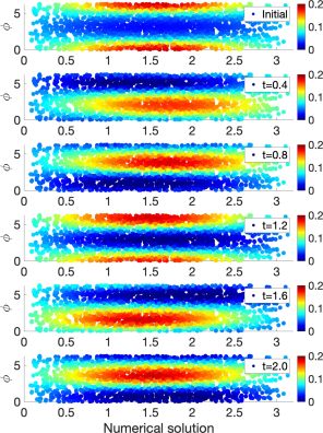
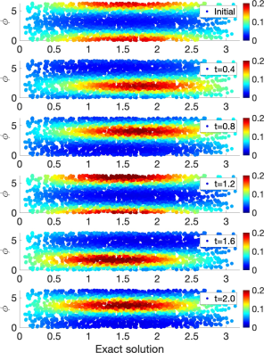
Figure 2. Left: The numerical solution $\rho^{k}_{i}$ in terms of $\theta,\varphi$ over $2000$ points $\{\mathbf{y}_{i}\}_{i=1}^{2000}\subset S^{2}\subset\mathbb{R}^{3}$. Right: The exact solution given by the oscillated von Mises–Fisher distribution ${\rho_{v}}(\theta,\varphi,t)$ in (4.4). We plot 6 snapshots at $t=0,0.4,0.8,1.2,1.6,2.0$.

4.2. Example I: Fokker-Planck evolution on dumbbell.

Suppose $(\theta,\phi)\in[0,2\pi)\times[0,\pi)$, then we have the following dumbbell in $\mathbb{R}^{200}$ parametrized as $(x,y,z,0,\cdots,0)=f_{1}(\theta,\phi)\in\mathbb{R}^{200}$, where

(4.9) $$r=\sqrt{\sqrt{1+0.95^{4}(\cos(2\phi)^{2}-1)}+0.95^{2}\cos(2\phi)}$$

$$x=r\sin(\phi)\cos(\theta),\quad y=r\sin(\phi)\sin(\theta),\quad z=r\cos(\phi).$$

After composition with a dilation and rotation map $f_{2}$ of $\mathbb{R}^{200}$ , we have an embedded dumbbell $\mathcal{M}\subset\mathbb{R}^{200}$. Suppose $f_{2}\circ f_{1}(\theta,\phi)$ is the parametrization of $\mathcal{M}$. We sample $4000$ points $(\theta_{1},\phi_{1}),\cdots,(\theta_{4000},\phi_{4000})$ on $[0,2\pi)\times[0,\pi)$. Let $\mathbf{x}_{i}=f_{2}\circ f_{1}(\theta_{i},\phi_{i})$, then we have a non uniform sample $\{\mathbf{x}_{i}\}_{i=1}^{4000}$ on $\mathcal{M}$. We apply the diffusion map to find the reaction coordinates $\{\mathbf{y}_{i}\}_{i=1}^{4000}$ of $\{\mathbf{x}_{i}\}_{i=1}^{4000}$ in $\mathbb{R}^{3}$, i.e. $\{\mathbf{y}_{i}\}_{i=1}^{4000}$ can be regarded as a non uniform sample on a dumbbell $\mathcal{N}\subset\mathbb{R}^{3}$.

Suppose $\psi_{i}$ is the $i$ th eigenfunction of the Laplace-Beltrami operator on $\mathcal{N}$. Assume the initial density $\rho^{0}$ is $\psi_{2}$ plus some constant (so that $\rho^{0}$ is positive) as shown in Fig 3. Assume the equilibrium density $\pi$ is $\psi_{8}$ plus some constant as shown in Fig 3. We first obtain the approximated Voronoi cell volumes $|\tilde{C}_{i}|_{i=1}^{4000}$ and the areas $\tilde{\Gamma}_{ij}$ from Algorithm 1 by taking the bandwidth $r=0.16$ and threshold $s=0$. Then we adjust the initial data, i.e., we replace $\rho^{0}$ by $c\rho^{0}$ such that (3.107) holds. We set the time step $\Delta t=0.05$. Let $T=k\Delta t$ for the integer $k$ and $1\leq k\leq 20000$, i.e., we iterate the scheme for $20000$ times and set the final time to be $T=20000*\Delta t=1000.$ We use the unconditional stable explicit scheme (3.99) to solve $\rho^{k}$. We compare the numerical relative error in maximum norm with the theoretic relative error, $|\lambda_{2}|^{k}=0.9997^{k}$ in (3.111), in the semilog-plot in Fig 4. The exponential convergence rate is exactly same. To clearly see the dynamics of the change of the density over the $4000$ points, we plot $\rho^{k}$ for $k=20,60,100,160,220,4000$, correspondingly $T=1,3,5,8,11,200$ in Fig 5

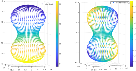
Figure 3. Left: The initial density is the second eigenfunction of the Laplace Beltrami operator on a dumbbell $\mathcal{N}\subset\mathbb{R}^{3}$ plus a constant. We plot it over $4000$ points $\{\mathbf{y}_{i}\}_{i=1}^{4000}\subset\mathcal{N}\subset\mathbb{R}^{3}$. Right: The equilibrium density is the eighth eigenfunction of the Laplace Beltrami operator on a dumbbell $\mathcal{N}\subset\mathbb{R}^{3}$ plus a constant. We plot it over $4000$ points $\{\mathbf{y}_{i}\}_{i=1}^{4000}\subset\mathcal{N}\subset\mathbb{R}^{3}$.

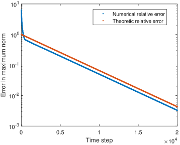
Figure 4. The semilog-plot comparison between the numerical relative error with theoretic relative error. The numerical relative error is the error from the unconditional stable explicit scheme (3.99) with $\Delta t=0.05$ and $1\leq k\leq 20000$. The theoretic relative error is based on (3.111) with $|\lambda_{2}|^{k}=0.9997^{k}$ .

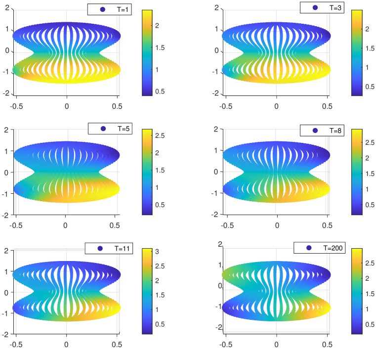
Figure 5. The density dynamics $\rho^{k}$ from the unconditional stable explicit scheme (3.99) with $\Delta t=0.05$. We plot $\rho^{k}$ for $k=20,60,100,160,220,4000$, correspondingly on time $T=1,3,5,8,11,200$.

4.3. Example II: Fokker-Planck evolution on Klein bottle.

Suppose $(\theta,\phi)\in[0,2\pi)\times[0,2\pi)$, then we have the following Klein bottle in $\mathcal{N}\subset\mathbb{R}^{4}$ parametrized as $(x,y,z,w)=f(\theta,\phi)\in\mathbb{R}^{4}$, where

(4.10) $$x=(1+0.3\cos(\theta))\cos(\phi)$$

$$y=(1+0.3\cos(\theta))\sin(\phi)$$

$$z=0.3\sin(\theta)\cos(\frac{\phi}{2})$$

$$w=0.3\sin(\theta)\sin(\frac{\phi}{2})$$

We sample $2000$ points $(\theta_{1},\phi_{1}),\cdots,(\theta_{2000},\phi_{2000})$ on $[0,2\pi)\times[0,2\pi)$. Let $\mathbf{y}_{i}=f(\theta_{i},\phi_{i})$, then we have non uniform samples $\{\mathbf{y}_{i}\}_{i=1}^{2000}$ on $\mathcal{N}$. We can regard them as the reaction coordinates of 2000 points sampled on $\mathcal{M}$ (a manifold diffeomorphic to a Klein bottle) in some high dimensional space. In this example, we will visualize the functions on the Klein bottle by two methods. First, consider the projection from $\mathbb{R}^{4}$ to $\mathbb{R}^{3}$ by $(x,y,z,w)\rightarrow(x,y,z)$. The restriction of the projection on $\mathcal{N}$ maps the Klein bottle to a pinched torus in $\mathbb{R}^{3}$. Second, consider the projection from $\mathbb{R}^{4}$ to $\mathbb{R}^{3}$ by $(x,y,z,w)\rightarrow(y,z,w)$. The restriction of the projection on $\mathcal{N}$ maps the Klein bottle to a Roman surface in $\mathbb{R}^{3}$. For any function on the Klein bottle, we will visualize it by plotting it on both the pinched torus and the Roman surface.

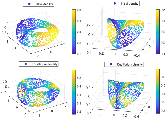
Figure 6. Top two panels: The initial density is the second eigenfunction of the Laplace Beltrami operator on a Klein bottle $\mathcal{N}\subset\mathbb{R}^{4}$ plus a constant. We plot it over the pinched torus and the roman surface in $\mathbb{R}^{3}$ respectively. Bottom two panels: The equilibrium density is the seventh eigenfunction of the Laplace Beltrami operator on a Klein bottle $\mathcal{N}\subset\mathbb{R}^{4}$ plus a constant. We plot it over the pinched torus and the roman surface in $\mathbb{R}^{3}$ respectively.

Suppose $\psi_{i}$ is the $i$ th eigenfunction of the Laplace-Beltrami operator on $\mathcal{N}$. Assume the initial density $\rho^{0}$ is $\psi_{2}$ plus some constant (so that $\rho^{0}$ is positive) as shown in Fig 6. Assume the equilibrium density $\pi$ is $\psi_{7}$ plus some constant as shown in Fig 6. We first obtain the approximated Voronoi cell volumes $|\tilde{C}_{i}|_{i=1}^{2000}$ and the areas $\tilde{\Gamma}_{ij}$ from Algorithm 1 by taking the bandwidth $r=0.23$ and threshold $s=0$. Then we adjust the initial data, i.e., we replace $\rho^{0}$ by $c\rho^{0}$ such that (3.107) holds. We set the time step $\Delta t=0.05$. Let $T=k\Delta t$ for the integer $k$ and $1\leq k\leq 10000$, i.e., we iterate the scheme for $10000$ times and set the final time to be $T=10000*\Delta t=500.$ We use the unconditional stable explicit scheme (3.99) to solve $\rho^{k}$. We compare the numerical relative error in maximum norm with the theoretic relative error, $|\lambda_{2}|^{k}=0.9993^{k}$ in (3.111), in the semilog-plot in Fig 7. The exponential convergence rate is exactly the same. To clearly see the dynamics of the change of the density over the $2000$ points, we plot $\rho^{k}$ for $k=50,1000,2000,10000$, correspondingly $T=2.5,50,100,500$ in Fig 8

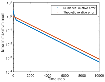
Figure 7. The semilog-plot comparison between the numerical relative error with theoretic relative error in the Klein bottle example. The numerical relative error is the error from the unconditional stable explicit scheme (3.99) with $\Delta t=0.05$ and $1\leq k\leq 10000$. The theoretic relative error is base on (3.111) with $|\lambda_{2}|^{k}=0.9993^{k}$.

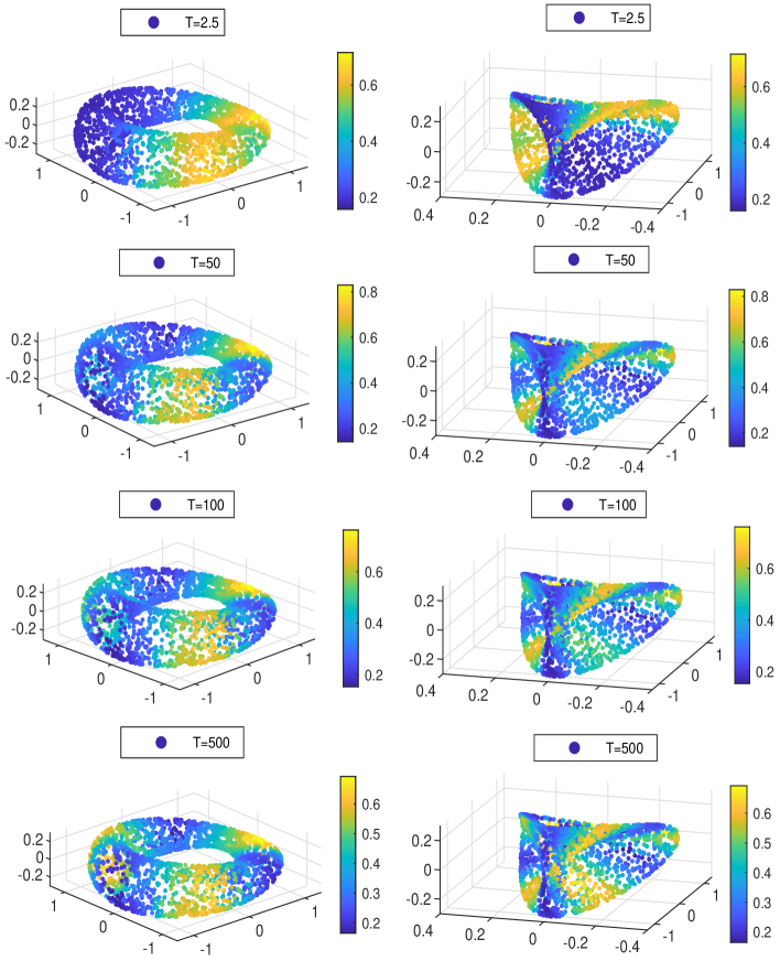
Figure 8. The density dynamics $\rho^{k}$ from the unconditional stable explicit scheme (3.99) with $\Delta t=0.05$. On the left four panels, we plot $\rho^{k}$ for $k=50,1000,2000,10000$ corresponding to time $T=2.5,50,100,500$ on the pinched torus. On the right four panels, we plot $\rho^{k}$ for $k=50,1000,2000,10000$ corresponding to time $T=2.5,50,100,500$ on the Roman surface.

4.4. Example III: The “breakup” of Pangaea via Fokker-Planck evolution on sphere.

In this example, we use the Fokker-Planck evolution on sphere to simulate the dynamics of the altitude of continents and the depth of oceans for earth based on the dataset for initial distribution of Pangaea supercontinent (250 million years ago) and the equilibrium distribution of the current earth.

Suppose $\{\mathbf{y}_{i}\}_{i=1}^{2000}$ are the points on the unit sphere $\mathcal{N}=S^{2}\subset\mathbb{R}^{3}$, i.e., $\{\mathbf{y}_{i}\}_{i=1}^{2000}$ are the reaction coordinates of $2000$ points on $\mathcal{M}$ (a manifold diffeomorphic to a sphere) in some high dimensional space. Assume the initial density $\rho^{0}_{i}$ at $\{\mathbf{y}_{i}\},\,i=1,\cdots,2000$ are extracted from the Pangaea continents map file [1] as shown in Fig 9 (down left). The value of the initial density $\rho^{0}_{i}\in\{1,2\}$ where $1$ represents oceans and $2$ represents continents. Assume the equilibrium $\{\pi_{i}\}$ at $\{\mathbf{y}_{i}\}$ are collected from the ETOPO5 topography data [2] expressing the altitude of continents and the depth of oceans for earth. The value of the equilibrium $\{\pi_{i}\}$ ranges from $-7000$ to $7000$ where the positive values represent the altitude of continents, negative values represent the depth of oceans and $0$ represents sea level. Before plugging into the Fokker-Planck equation, we add a constant $c_{p}$ to $\pi_{i}$ such that $\pi_{i}>0$ for all $i$. However, when showing the evolution of continents in figures, we subtract this constant and present the true physical altitudes.

We first obtain the approximated Voronoi cell volumes $|\tilde{C}_{i}|_{i=1}^{n}$ and areas $\tilde{\Gamma}_{ij}$ from Algorithm 1 by taking the bandwidth $r=0.3$ and threshold $s=0$. Then we adjust the initial data, i.e., we replace $\rho^{0}$ by $c\rho^{0}$ such that the total mass condition (3.107) holds. We set the time step $\Delta t=0.05$. Let $T=k\Delta t$ for the integer $k$ and $1\leq k\leq 10000$, i.e., we iterate the scheme for $10000$ times and set the final time to be $T=10000*\Delta t=500.$ We use the unconditionally stable explicit scheme (3.99) to solve $\rho^{k}$. In Fig 9 (up), the numerical relative error in maximum norm is semilog-plotted using circles. Compared with decay of the theoretic relative error $|\lambda_{2}|^{k}$ in (3.111), blue line in the semilog-plot, the exponential convergence rate is exactly same. The initial 3D plot of Pangaea continents is shown in Fig 9 (down left) while the final 3D plot at $T=500$ of the simulated altitude and depth of continents and oceans are shown in Fig 9 (down right). To clearly see the dynamics of altitude and depth of continents and oceans at $n$ points with longitude and latitude, starting from the same Pangaea continents with time step $\Delta t=0.05$, four snapshots at $T=0,1,10,75$ of the dynamics are shown in Fig 10. A video is also provided to show the dynamics of the density https://youtu.be/j5XBPdQhEEs. Here we used nonuniform time intervals since the shapes of continentals (the region with positive altitudes) quickly move from the initial Pangaea supercontinents towards the equilibrium shape of current continents. If we only care about the shape of the continents and keep the binary-valued density during the shape evolution, we refer to [27] for the thresholding adjustment method.

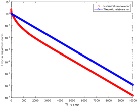
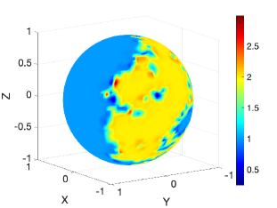
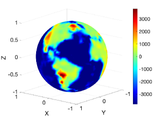
Figure 9. Simulations for the density dynamics of altitude and depth of continents and oceans starting from pangaea (down left) to the final altitude of land-ocean (down right) with parameters $\,\mathrm{d}t=0.05$, $T=500$. (up)The semilog-plot comparison between the numerical relative error in maximum norm (blue circle) with theoretic relative error $|\lambda_{2}|^{k}=0.9985^{k}$ (blue line) in (3.111).

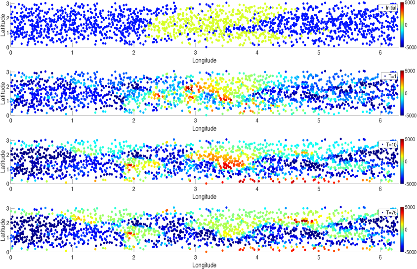
Figure 10. 2D Snapshots for the density dynamics of altitude and depth of continents and oceans at $2000$ points with longitude and latitude starting from Pangaea with parameters $\,\mathrm{d}t=0.05$, $T=0,1,10,75$.

5. Discussion

We focus on the analysis of the dynamics of a physical system with a manifold structure. The underlying manifold structure of the system is reflected through a point cloud in a high dimensional space. By applying the diffusion map, we find the reaction coordinates so that those data points are reduced onto a manifold in a low dimensional space. Based on the reaction coordinates, we propose an implementable, unconditionally stable, finite volume scheme for a Fokker-Planck equation which incorporates both the structure of the manifold in the low dimensional space and the equilibrium information. The finite volume scheme defines an approximated Markov process (random walk) on the point cloud with an approximated transition probability and jump rate. We also provide the weighted $L^{2}$ convergence analysis of the finite volume scheme to the Fokker-Planck equation on the manifold in the low dimensional space. The efficiency, unconditional stability, and accuracy of the data-driven solver proposed in this paper are justified theoretically. Although we construct several numerical examples to illustrate our data-driven solver, there are still many interesting directions issued from practical problems for future works. An important direction is the manifold-related applications such as the optimal network partitions and the transition path in chemical reactions, especially on the high dimensional practical datasets.

Appendix A Theorems about embedding by eigenfunctions of Laplacian

Let $\Delta$ be the Laplace-Beltrami operator of a closed smooth Riemannian manifold $\mathcal{M}$. Let $\{\lambda_{i}\}_{i=0}^{\infty}$ be the eigenvalues of $-\Delta$, and

(A.1) $$\Delta\psi_{i}=-\lambda_{i}\psi_{i},$$

where $\psi_{i}$ is the corresponding eigenfunction normalized in $L^{2}(\mathcal{M})$. We have $0=\lambda_{0}<\lambda_{1}\leq\lambda_{2}\leq\cdots$.

In this section, we review the theorems about embedding the manifold $\mathcal{M}$ by using the eigenfunctions of $\Delta$. In [7], the authors provide a theorem about spectral embedding by using all the eigenvalues and eigenfunctions of $\Delta$ into the Hilbert space $\ell^{2}$.

Theorem A.1.

(Bérard-Besson-Gallot, [7]) Let $M$ be a $d$ dimensional smooth closed Riemannian manifold. Then, for $\mathbf{x}\in\mathcal{M}$

(A.2) $$\Psi(\mathbf{x})=(2t)^{\frac{d+2}{4}}\sqrt{2}(4\pi)^{\frac{d}{4}}(e^{-\lambda_{1}t}\psi_{1}(\mathbf{x}),\cdots,e^{-\lambda_{q}t}\psi_{q}(\mathbf{x}),\cdots),$$

is an embedding of $M$ into $\ell^{2}$ for all $t>0$.

[36] improves the above result locally. They show that one can use finite eigenfunctions of Laplace-Beltrami operator to embed the manifold locally. The result can be briefly summarized as follows.

Theorem A.2.

(Jones-Maggioni-Schul, [36]) Let $\mathcal{M}$ be a $d$ dimensional smooth closed Riemannian manifold, for each $\mathbf{x}\in M$, there are $j_{1}\leq\cdots\leq j_{d}$ and the constants $C_{1},\cdots,C_{d}$ such that

(A.3) $$\Psi(\mathbf{x})=(C_{1}\psi_{j_{1}}(\mathbf{x}),\cdots,C_{d}\psi_{j_{d}}(\mathbf{x})),$$

is locally a bi-Lipschitz chart.

Moreover, the next theorem [46] says that we can use the eigenvalues and eigenfunctions of the Laplace-Beltrami operator to construct an almost isometric embedding of the manifold into some Euclidean space.

Theorem A.3.

(Portegies, [46]) Let $\mathcal{M}$ be a $d$ dimensional smooth closed Riemannian manifold. Suppose $\operatorname{Ric}_{\mathcal{M}}\geq(d-1)k$, the injectivity radius of $\mathcal{M}$, $i(\mathcal{M})\geq i_{0}$ and the volume of $\mathcal{M}$, $\operatorname{Vol}(\mathcal{M})\leq V$. For any $\epsilon>0$, there is a $\mathbf{t}_{0}(\epsilon,d,k,i_{0})$ such that for $t<\mathbf{t}_{0}$, there is $C(\epsilon,d,k,i_{0},V,t)$, if $q>C$, then for $\mathbf{x}\in\mathcal{M}$

(A.4) $$\Psi(\mathbf{x})=(2t)^{\frac{d+2}{4}}\sqrt{2}(4\pi)^{\frac{d}{4}}(e^{-\lambda_{1}t}\psi_{1}(\mathbf{x}),\cdots,e^{-\lambda_{q}t}\psi_{q}(\mathbf{x})),$$

is an embedding of $\mathcal{M}$ into $\mathbb{R}^{q}$ such that $1-\epsilon<\|\nabla\Psi\|_{op}<1+\epsilon$. Here $\|\cdot\|_{op}$ is the operator norm.

Based on Theorem 2.7, the smallest $q$ that

(A.5) $$\Psi_{1}(\mathbf{x})=(\psi_{1}(\mathbf{x}),\cdots,\psi_{q}(\mathbf{x})),$$

is a smooth embedding of $\mathcal{M}$ is called the embedding dimension of $\mathcal{M}$. Based on Theorem A.3, the smallest $q$ that

(A.6) $$\Psi_{2}(\mathbf{x})=(2t)^{\frac{d+2}{4}}\sqrt{2}(4\pi)^{\frac{d}{4}}(e^{-\lambda_{1}t}\psi_{1}(\mathbf{x}),\cdots,e^{-\lambda_{q}t}\psi_{q}(\mathbf{x})),$$

is an almost isometric embedding of $\mathcal{M}$ is called the almost isometric embedding dimension of $\mathcal{M}$. We expect the embedding dimension is much smalled than the almost isometric embedding dimension. Hence, for the dimension reduction purpose, we are looking for an embedding of the manifold rather than an almost isometric embedding.

Appendix B Proof of Proposition 3.2

Since $\delta$ is less than the injectivity radius, there is a Euclidean ball $B^{T_{y_{i}}\mathcal{N}}_{\delta}(0)$ of radius $\delta$ in the tangent space $T_{y_{i}}\mathcal{N}$ of $\mathcal{N}$ at $\mathbf{y}_{i}$ such that the exponential map $\exp_{y_{i}}:B^{T_{y_{i}}\mathcal{N}}_{\delta}(0)\rightarrow B_{\delta}(\mathbf{y}_{i})$ is a diffeomorphism. Suppose $y_{j}=\exp_{y_{i}}(w)$. We illustrate this setup in Figure 11. It is sufficient to prove that $\exp_{y_{i}}^{-1}(B_{\delta}(\mathbf{y}_{i})\cap G_{ij})$ is a $d-1$ dimensional submanifold of $T_{y_{i}}\mathcal{N}$. For any $v\in\exp_{y_{i}}^{-1}(B_{\delta}(\mathbf{y}_{i})\cap G_{ij})$, by the definition of the bisector, we have

(B.1) $$d^{2}_{\mathcal{N}}(\exp_{y_{i}}(v),\exp_{y_{i}}(w))=d^{2}_{\mathcal{N}}(\exp_{y_{i}}(v),y_{j})=d^{2}_{\mathcal{N}}(\exp_{y_{i}}(v),y_{i})=|v|^{2}.$$

Note that

(B.2) $$d^{2}_{\mathcal{N}}(\exp_{y_{i}}(v),\exp_{y_{i}}(w))=|v-w|^{2}+f(v,w).$$

$f(v,w)$ is a smooth function on $B^{T_{y_{i}}\mathcal{N}}_{\delta}(0)\times B^{T_{y_{i}}\mathcal{N}}_{\delta}(0)$. In particular,

(B.3) $$f(v,w)=-\frac{1}{3}R_{y_{i}}(v,w,v,w)+O((|v|^{2}+|w|^{2})^{\frac{5}{2}})$$

for $|v|$ and $|w|$ small, where $R_{y_{i}}$ is the curvature tensor at $y_{i}$. Combine (B.1) and (B.2), we have that

(B.4) $$|w|^{2}-2v\cdot w+f(v,w)=0.$$

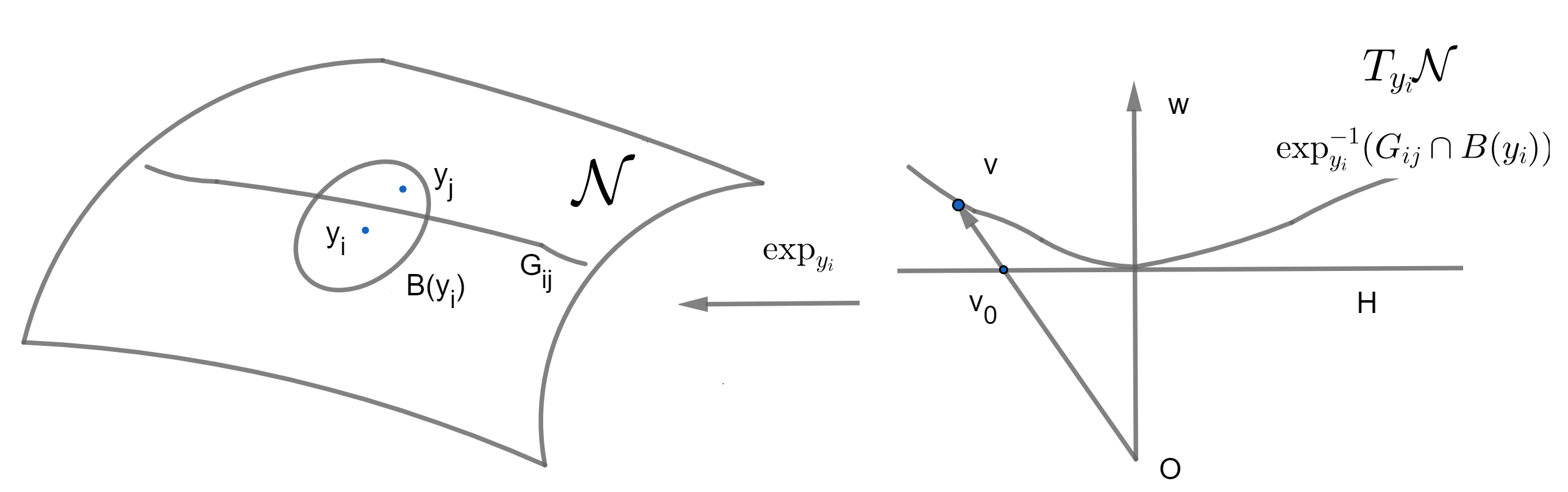
Figure 11. An illustration to the proof of Proposition 3.2

As $y_{j}$ is a fixed point, we treat $w$ as a fixed vector. Therefore, we use the notation $f_{w}(x)=f(x,w)$ to indicate $f_{w}$ is a function of $x\in B^{T_{y_{i}}\mathcal{N}}_{\delta}(0)$. Then, we can define a smooth function $F(t,x)$ on $\mathbb{R}\times B^{T_{y_{i}}\mathcal{N}}_{\delta}(0)$ as

(B.5) $$F(t,x)=|w|^{2}-2(1+t)x\cdot w+f_{w}((1+t)x).$$

Let $H$ be the $d-1$ dimensional hyperplane that perpendicularly bisects $w$ in $T_{y_{i}}\mathcal{N}$. Let $v_{0}$ be the vector on $H$ so that $v=(1+t_{0})v_{0}$. By (B.4), $F(t_{0},v_{0})=0$. If we can show that $\frac{\partial F(t_{0},v_{0})}{\partial t}\not=0$, then by the Implicit Function Theorem, there is a ball $B$ centered at $v_{0}$ so that $t=g(x)$ for $x\in B$ and $g$ is differentiable. Hence, $(1+g(x))x$ for $x\in B\cap H$ is a chart for $\exp_{y_{i}}^{-1}(B_{\delta}(\mathbf{y}_{i})\cap G_{ij})$ around $v$. We calculate $\frac{\partial F(t_{0},v_{0})}{\partial t}$:

(B.6) $$\frac{\partial F(t_{0},v_{0})}{\partial t}=-2v_{0}\cdot w+\nabla f_{w}(v)\cdot v_{0}.$$

By (B.3), $|\nabla f_{w}(v)|=O(|v||w|^{2})$ where the constant depends on the sectional curvatures at $\mathbf{y}_{i}$. Since the manifold is compact, the sectional curvatures have upper and lower bounds. Hence,

(B.7) $$\frac{\partial F(t_{0},v_{0})}{\partial t}=-2v_{0}\cdot w+\nabla f_{w}(v)\cdot v_{0}<-2|v_{0}||w|\cos(\theta)+|v_{0}|O(|v||w|^{2}),$$

where $\theta$ is the angle between $v_{0}$ and $w$. Since $v_{0}\in B^{T_{y_{i}}\mathcal{N}}_{\delta}(0)\cap H$, $\cos(\theta)>\frac{|w|}{2\delta}$. $v\in B^{T_{y_{i}}\mathcal{N}}_{\delta}(0)$, so $|v|<\delta$. Therefore, when $\delta$ is small enough,

(B.8) $$\frac{\partial F(t_{0},v_{0})}{\partial t}<|v_{0}||w|^{2}(-\frac{1}{\delta}+O(\delta))<0.$$

Next, we prove the second part of the proposition. $\mathbf{y}^{*}\in M_{ij}$ follows from the construction. Note that by the triangle inequality and the definition of the bisector, the geodesic sphere centered at $\mathbf{y}_{i}$ through $\mathbf{y}^{*}$ is tangent to $M_{ij}$ at $\mathbf{y}^{*}$. Hence, by Gauss’s Lemma, the minimizing geodesic between $y_{i}$ and $y_{j}$ is perpendicular to $M_{ij}$ at $\mathbf{y}^{*}$.

Appendix C Proof of Proposition 3.12 and Proposition 3.13

We start from a study of the matrix $C_{n,r}(\mathbf{y}_{k})$ in Definition 3.8 and relate it to its continuous form. Consider the local covariance matrix $C_{\mathbf{y}_{k},B^{\mathbb{R}^{\ell}}_{\sqrt{r}}(\mathbf{y}_{k})\cap\mathcal{N}}$ defined as follows.

(C.1) $$C_{\mathbf{y}_{k},B^{\mathbb{R}^{\ell}}_{\sqrt{r}}(\mathbf{y}_{k})\cap\mathcal{N}}= \int_{B^{\mathbb{R}^{\ell}}_{\sqrt{r}}(\mathbf{y}_{k})\cap\mathcal{N}}(\mathbf{y}-\mathbf{y}_{k})(\mathbf{y}-\mathbf{y}_{k})^{\top}\rho^{**}(\mathbf{y})dV_{\mathcal{N}}(\mathbf{y})\in\mathbb{R}^{\ell\times\ell}.$$

Suppose $C_{\mathbf{y}_{k},B^{\mathbb{R}^{\ell}}_{\sqrt{r}}(\mathbf{y}_{k})\cap\mathcal{N}}$ has the following eigendecomposition:

(C.2) $$C_{\mathbf{y}_{k},B^{\mathbb{R}^{\ell}}_{\sqrt{r}}(\mathbf{y}_{k})\cap\mathcal{N}}=U(\mathbf{y}_{k})\Lambda(\mathbf{y}_{k})U(\mathbf{y}_{k})^{\top}\in O(\ell),$$

where $\Lambda(\mathbf{y}_{k})$ is a diagonal matrix with the diagonal entries to be eigenvalues of $C_{\mathbf{y}_{k},B^{\mathbb{R}^{\ell}}_{\sqrt{r}}(\mathbf{y}_{k})\cap\mathcal{N}}$. Moreover, we have $\Lambda_{11}(\mathbf{y}_{k})\geq\Lambda_{22}(\mathbf{y}_{k})\geq\cdots\geq\Lambda_{\ell\ell}(\mathbf{y}_{k})$. $U(\mathbf{y}_{k})\in O(\ell)$ consists of the corresponding orthonormal eigenvectors of $C_{\mathbf{y}_{k},B^{\mathbb{R}^{\ell}}_{\sqrt{r}}(\mathbf{y}_{k})\cap\mathcal{N}}$. Intuitively, $C_{\mathbf{y}_{k},B^{\mathbb{R}^{\ell}}_{\sqrt{r}}(\mathbf{y}_{k})\cap\mathcal{N}}$ is the continuous form of the matrix $C_{n,r}(\mathbf{y}_{k})$.

By setting $\epsilon=\sqrt{r}$ in Proposition 3.2 in [56], we have the following lemma.

Lemma C.1.

Assume that $T_{\mathbf{y}_{k}}\mathcal{N}$ is generated by the first $d$ standard basis of $\mathbb{R}^{\ell}$.

(C.3) $$\Lambda(\mathbf{y}_{k}) =\frac{|S^{d-1}|P(\mathbf{y}_{k})r^{\frac{d+2}{2}}}{d(d+2)}\Big{(}\begin{bmatrix}I_{d\times d}&0\\ 0&0\\ \end{bmatrix}+O(r)\Big{)},$$

(C.4) $$U(\mathbf{y}_{k}) =\begin{bmatrix}X_{1}&0\\ 0&X_{2}\\ \end{bmatrix}+O(r),$$

where $X_{1}\in O(d)$ and $X_{2}\in O(\ell-d)$.

Above lemma says that the first $d$ eigenvectors of $C_{\mathbf{y}_{k},B^{\mathbb{R}^{\ell}}_{\sqrt{r}}(\mathbf{y}_{k})\cap\mathcal{N}}$ form an orthonormal basis of $T_{\mathbf{y}_{k}}\mathcal{N}$ up to an error of order $O(r)$. Note that, for simplicity, we assume $T_{\mathbf{y}_{k}}\mathcal{N}$ is generated by the first $d$ standard basis of $\mathbb{R}^{\ell}$ so that $U(\mathbf{y}_{k})$ can be expressed in the above block form. Suppose $C_{n,r}(\mathbf{y}_{k})$ has the following eigendecomposition:

(C.5) $$C_{n,r}(\mathbf{y}_{k})=U_{n}(\mathbf{y}_{k})\Lambda_{n}(\mathbf{y}_{k})U_{n}(\mathbf{y}_{k})^{\top}.$$

$\Lambda_{n}(\mathbf{y}_{k})$ is a diagonal matrix with the diagonal entries to be eigenvalues of $C_{n,r}(\mathbf{y}_{k})$. Moreover, we have $\Lambda_{n,11}(\mathbf{y}_{k})\geq\Lambda_{n,22}(\mathbf{y}_{k})\geq\cdots\geq\Lambda_{n,\ell\ell}(\mathbf{y}_{k})$. $U_{n}(\mathbf{y}_{k})\in O(\ell)$ consists of the corresponding orthonormal eigenvectors of $C_{n,r}(\mathbf{y}_{k})$.

The relation between the eigenstructure of $C_{\mathbf{y}_{k},B^{\mathbb{R}^{\ell}}_{\sqrt{r}}(\mathbf{y}_{k})\cap\mathcal{N}}$ and $C_{n,r}(\mathbf{y}_{k})$ is discussed in Lemma E.4 in [56].

Lemma C.2.

Assume that $T_{\mathbf{y}_{k}}\mathcal{N}$ is generated by the first $d$ standard basis of $\mathbb{R}^{\ell}$. When $n$ is large enough, with probability greater than $1-\frac{1}{n^{2}}$, for all $\mathbf{y}_{k}$,

(C.6) $$\Lambda_{n}(\mathbf{y}_{k}) =\Lambda(\mathbf{y}_{k})+O(\sqrt{\frac{\log n}{nr^{-\frac{d}{2}-2}}}),$$

(C.7) $$U_{n}(\mathbf{y}_{k}) =\begin{bmatrix}X^{\prime}_{1}&0\\ 0&X^{\prime}_{2}\\ \end{bmatrix}U(\mathbf{y}_{k})+O(\sqrt{\frac{\log n}{nr^{\frac{d}{2}-2}}}),$$

where $X^{\prime}_{1}\in O(d)$ and $X^{\prime}_{2}\in O(\ell-d)$.

Remark C.3.

Above lemma follows from Lemma E.4 in [56] if we choose $\epsilon=\sqrt{r}$ and $\rho\rightarrow\infty$ in Case 0 of Lemma E.4 in [56]. In fact, Case 0 of Lemma E.4 in [56] focuses on the first $d$ eigenpairs of the matrix $C_{\mathbf{y}_{k},B^{\mathbb{R}^{\ell}}_{\sqrt{r}}(\mathbf{y}_{k})\cap\mathcal{N}}$ of which we need to recover.

If we combine Lemma C.1 and Lemma C.2, we have

(C.8) $$\Lambda_{n}(\mathbf{y}_{k}) =\frac{|S^{d-1}|P(\mathbf{y}_{k})r^{\frac{d+2}{2}}}{d(d+2)}\begin{bmatrix}I_{d\times d}&0\\ 0&0\\ \end{bmatrix}+O(r^{\frac{d}{2}+2})+O(\sqrt{\frac{\log n}{nr^{-\frac{d}{2}-2}}}),$$

(C.9) $$U_{n}(\mathbf{y}_{k}) =\begin{bmatrix}U_{1}&0\\ 0&U_{2}\\ \end{bmatrix}+O(r)+O(\sqrt{\frac{\log n}{nr^{\frac{d}{2}-2}}}),$$

where $U_{1}\in O(d)$ and $U_{2}\in O(\ell-d)$. If $\frac{nr^{\frac{d}{2}}}{\log n}\rightarrow\infty$ as $n\rightarrow\infty$, then $\sqrt{\frac{\log n}{nr^{\frac{d}{2}-2}}}\leq r$. If $\frac{nr^{\frac{d}{2}+2}}{\log n}\rightarrow\infty$ as $n\rightarrow\infty$, then $\sqrt{\frac{\log n}{nr^{\frac{d}{2}-2}}}\leq r$ and $\sqrt{\frac{\log n}{nr^{-\frac{d}{2}-2}}}\leq r^{\frac{d}{2}+2}$. Hence, we have the following proposition.

Proposition C.4.

Assume that $T_{\mathbf{y}_{k}}\mathcal{N}$ is generated by the first $d$ standard basis of $\mathbb{R}^{\ell}$. If $\frac{nr^{\frac{d}{2}}}{\log n}\rightarrow\infty$ as $n\rightarrow\infty$, then with probability greater than $1-\frac{1}{n^{2}}$, for all $\mathbf{y}_{k}$,

(C.10) $$U_{n}(\mathbf{y}_{k}) =\begin{bmatrix}U_{1}&0\\ 0&U_{2}\\ \end{bmatrix}+O(r),$$

where $U_{1}\in O(d)$ and $U_{2}\in O(\ell-d)$.

If $\frac{nr^{\frac{d}{2}+2}}{\log n}\rightarrow\infty$ as $n\rightarrow\infty$, then with probability greater than $1-\frac{1}{n^{2}}$, for all $\mathbf{y}_{k}$,

(C.11) $$\Lambda_{n}(\mathbf{y}_{k}) =\frac{|S^{d-1}|P(\mathbf{y}_{k})r^{\frac{d+2}{2}}}{d(d+2)}\begin{bmatrix}I_{d\times d}&0\\ 0&0\\ \end{bmatrix}+O(r^{\frac{d}{2}+2}),$$

(C.12) $$U_{n}(\mathbf{y}_{k}) =\begin{bmatrix}U_{1}&0\\ 0&U_{2}\\ \end{bmatrix}+O(r),$$

where $U_{1}\in O(d)$ and $U_{2}\in O(\ell-d)$.

Above proposition should be understood in the following way. If $n$ and $r$ satisfy $\frac{nr^{\frac{d}{2}}}{\log n}\rightarrow\infty$ as $n\rightarrow\infty,$ then we have an approximation of the tangent space of $\mathcal{N}$ at $\mathbf{y}_{k}$, i.e. the first $d$ eigenvectors of $C_{n,r}(\mathbf{y}_{k})$ are the basis of $T_{\mathbf{y}_{k}}\mathcal{N}$ up to an error of order $O(r)$. If $n$ and $r$ satisfy $\frac{nr^{\frac{d}{2}+2}}{\log n}\rightarrow\infty$ as $n\rightarrow\infty$, the first $d$ eigenvectors of $C_{n,r}(\mathbf{y}_{k})$ are the basis of $T_{\mathbf{y}_{k}}\mathcal{N}$ up to an error of order $O(r)$. Moreover, there are $d$ significantly large eigenvalues of $C_{n,r}(\mathbf{y}_{k})$ which are close to the first $d$ eigenvalues of $C_{\mathbf{y}_{k},B^{\mathbb{R}^{\ell}}_{\sqrt{r}}(\mathbf{y}_{k})\cap\mathcal{N}}$.

Next, we show that the map $\tilde{\iota}_{k}$ in the definition 3.8 restricted on $B^{\mathbb{R}^{\ell}}_{r}(\mathbf{y}_{k})\cap\mathcal{N}$ is a $1+O(r)$ bi-Lipschitz homeomorphism.

Lemma C.5.

Suppose $r\rightarrow 0$ and $\frac{nr^{\frac{d}{2}}}{\log n}\rightarrow\infty$ as $n\rightarrow\infty$. Suppose $r$ is small enough, then with probability greater than $1-\frac{1}{n^{2}}$, for all $\mathbf{y}_{k}$ and any $\mathbf{y},\mathbf{y}^{\prime}\in B^{\mathbb{R}^{\ell}}_{r}(\mathbf{y}_{k})\cap\mathcal{N}$, we have

(C.13) $$\|\tilde{\iota}_{k}(\mathbf{y}^{\prime})-\tilde{\iota}_{k}(\mathbf{y})\|_{\mathbb{R}^{d}}=\|\iota_{k}(\mathbf{y}^{\prime}-\mathbf{y})\|_{\mathbb{R}^{d}}=d_{\mathcal{N}}(\mathbf{y},\mathbf{y}^{\prime})(1+O(r)).$$

Proof.

$\|\tilde{\iota}_{k}(\mathbf{y}^{\prime})-\tilde{\iota}_{k}(\mathbf{y})\|_{\mathbb{R}^{d}}=\|\iota_{k}(\mathbf{y}^{\prime}-\mathbf{y})\|_{\mathbb{R}^{d}}$ follows from the definition. Next, we prove $\|\iota_{k}(\mathbf{y}^{\prime}-\mathbf{y})\|_{\mathbb{R}^{d}}=d_{\mathcal{N}}(\mathbf{y},\mathbf{y}^{\prime})(1+O(r))$. For simplicity, we assume $\mathbf{y}_{k}=0$ and $T_{\mathbf{y}_{k}}\mathcal{N}$ is generated by the first $d$ standard basis of $\mathbb{R}^{\ell}$. For any $\mathbf{y}\in\mathbb{R}^{\ell}$, we use the following notation to simplify the proof:

(C.14) $$\mathbf{y}=[\![v,\,v^{\bot}]\!]\in\mathbb{R}^{\ell}\,,$$

where $v\in T_{\mathbf{y}_{k}}\mathcal{N}$ forms the first $d$ coordinates of $y$ and $v^{\bot}\in T^{\bot}_{\mathbf{y}_{k}}\mathcal{N}$ forms the last $\ell-d$ coordinates of $\mathbf{y}$. For any $\mathbf{y},\mathbf{y}^{\prime}\in B^{\mathbb{R}^{\ell}}_{r}(\mathbf{y}_{k})\cap\mathcal{N}$, suppose $\mathbf{y}=[\![v_{1},\,v_{1}^{\bot}]\!]$ and $\mathbf{y}^{\prime}=[\![v_{2},\,v_{2}^{\bot}]\!]$. Due to the manifold structure of $\mathcal{N}$, we have

(C.15) $$\|v_{1}^{\bot}-v_{2}^{\bot}\|_{\mathbb{R}^{\ell-d}}\leq\mathcal{C}_{1}r\|v_{1}-v_{2}\|_{\mathbb{R}^{d}},$$

for some constant $\mathcal{C}_{1}$ depending on the curvature of $\mathcal{N}$. Hence,

(C.16) $$\|v_{1}-v_{2}\|_{\mathbb{R}^{d}}\leq\|\mathbf{y}^{\prime}-\mathbf{y}\|_{\mathbb{R}^{\ell}}\leq\|v_{1}-v_{2}\|_{\mathbb{R}^{d}}\sqrt{1+\mathcal{C}^{2}_{1}r^{2}},$$

which is equivalent to

(C.17) $$\|v_{1}-v_{2}\|_{\mathbb{R}^{d}}=\|\mathbf{y}^{\prime}-\mathbf{y}\|_{\mathbb{R}^{\ell}}(1+O(r^{2})).$$

Moreover, suppose $\{\beta_{n,r,1},\cdots,\beta_{n,r,d}\}$ are orthonormal eigenvectors corresponding to $C_{n,r}(\mathbf{y}_{k})$’s largest $d$ eigenvalues. Then, by Proposition C.4

(C.18) $$\beta_{n,r,1}=[\![\beta_{i},0]\!]+O(r),$$

where $\{\beta_{i}\}_{i=1}^{d}$ form an orthonormal basis of $T_{\mathbf{y}_{k}}\mathcal{N}\approx\mathbb{R}^{d}$.

(C.19) $$\|\iota_{k}(\mathbf{y}^{\prime}-\mathbf{y})\|_{\mathbb{R}^{d}}= \|v_{1}-v_{2}\|_{\mathbb{R}^{d}}+\|\mathbf{y}^{\prime}-\mathbf{y}\|_{\mathbb{R}^{\ell}}O(r)$$

$$= \|\mathbf{y}^{\prime}-\mathbf{y}\|_{\mathbb{R}^{\ell}}(1+O(r^{2}))+\|\mathbf{y}^{\prime}-\mathbf{y}\|_{\mathbb{R}^{\ell}}O(r)=\|\mathbf{y}^{\prime}-\mathbf{y}\|_{\mathbb{R}^{\ell}}(1+O(r)),$$

where we apply (C.17) in the second last step.

By equation (3.76), we know that $d_{\mathcal{N}}(y,\mathbf{y}^{\prime})\leq 2D_{1}r$. Hence, by Lemma 3.9,

(C.20) $$\|\iota_{k}(\mathbf{y}^{\prime}-\mathbf{y})\|_{\mathbb{R}^{d}}= \|\mathbf{y}^{\prime}-\mathbf{y}\|_{\mathbb{R}^{\ell}}(1+O(r))=d_{\mathcal{N}}(\mathbf{y},\mathbf{y}^{\prime})(1+O(d^{2}_{\mathcal{N}}(\mathbf{y},\mathbf{y}^{\prime})))(1+O(r))$$

$$= d_{\mathcal{N}}(\mathbf{y},\mathbf{y}^{\prime})(1+O(r^{2}))(1+O(r))=d_{\mathcal{N}}(\mathbf{y},\mathbf{y}^{\prime})(1+O(r)).$$

∎

We introduce the following notations to prove the following lemma and proposition. Denote the boundary of $C_{k}$ by $\partial C_{k}$. Denote the boundary of $\tilde{\iota}_{k}(C_{k})$ by $\partial\tilde{\iota}_{k}(C_{k})=\tilde{\iota}_{k}(\partial C_{k})$. Let $\tilde{C}_{k,0}$ be the Voronoi cell in $\mathbb{R}^{d}$ containing $0$ constructed in the Step 4 in Algorithm 1. Denote the boundary of $\tilde{C}_{k,0}$ by $\partial\tilde{C}_{k}$. Denote $d^{\mathbb{R}^{d}}_{\mathcal{H}}(S_{1},S_{2})$ be the Hausdorff distance between two sets $S_{1}$ and $S_{2}$ in $\mathbb{R}^{d}$ with respect to the Euclidean metric.

Lemma C.6.

If $n$ is large enough, for $r$ satisfying Assumption 3.10, with probability greater than $1-\frac{1}{n^{2}}$, for all $\mathbf{y}_{k}$ , $d^{\mathbb{R}^{d}}_{\mathcal{H}}(\partial\tilde{\iota}_{k}(C_{k}),\partial\tilde{C}_{k})=O(r^{2})$.

Proof.

For simplicity, in this proof, we use $|\cdot|$ to denote $\|\cdot\|_{\mathbb{R}^{d}}$. Based on Assumption 3.10, the requirement of Lemma C.5 holds. Recall that in Assumption 3.10, we assume $B^{\mathbb{R}^{\ell}}_{r}(\mathbf{y}_{k})\cap\{\mathbf{y}_{i}\}_{i=1}^{n}=\{\mathbf{y}_{k,1},\cdots,\mathbf{y}_{k,N_{k}}\}$. We have $C_{k}\subset B^{\mathbb{R}^{\ell}}_{r}(\mathbf{y}_{k})$. Moreover, if $\Gamma_{kj}$ is a Voronoi surface of $C_{k}$ between $\mathbf{y}_{k}$ and $\mathbf{y}_{j}$, then $\mathbf{y}_{j}\in B^{\mathbb{R}^{\ell}}_{r}(\mathbf{y}_{k})$. We denote $\Gamma_{k,i}$ to be the Voronoi face between $\mathbf{y}_{k}$ and $\mathbf{y}_{k,i}$.

The proof has two steps, first we show that for any $v\in\partial\tilde{\iota}_{k}(C_{k})$, $d_{\mathbb{R}^{d}}(v,\partial\tilde{C}_{k})=O(r^{2})$. We need to consider two cases in this step.

Case 1: $v\in\tilde{C}_{k,0}$

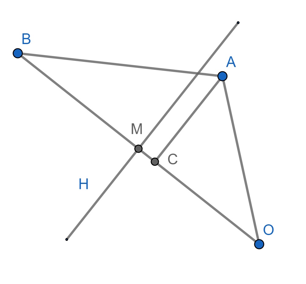
(a) The Case when $v=A\in\tilde{C}_{k,0}$

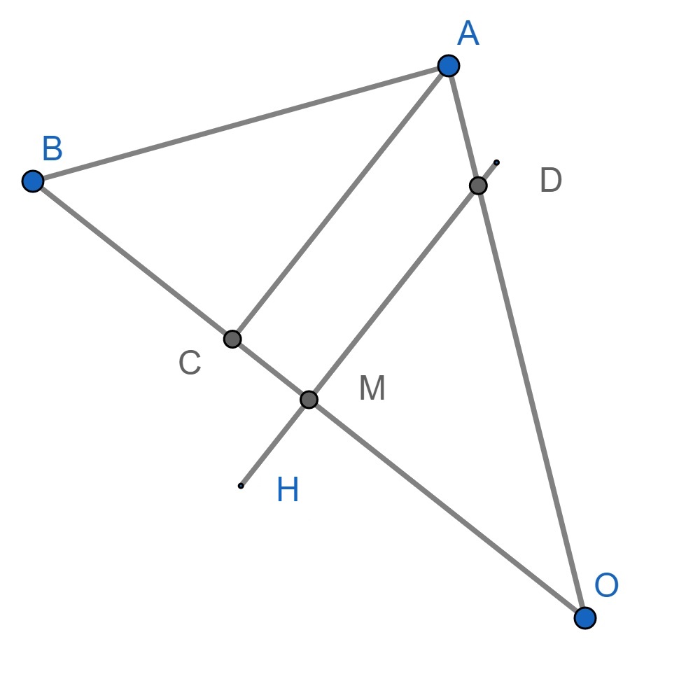
(b) The Case when $v=A\not\in\tilde{C}_{k,0}$

Figure 12. Illustrations of Case 1 and Case 2 in the proof of Lemma C.6.

Suppose $v=\tilde{\iota}_{k}(\mathbf{y})$ for some $\mathbf{y}\in\partial C_{k}$. Moreover $\mathbf{y}\in\Gamma_{k,i}$. In other word, $\mathbf{y}$ is on the Voronoi face between $\mathbf{y}_{k}$ and $\mathbf{y}_{k,i}\in B^{\mathbb{R}^{\ell}}_{r}(\mathbf{y}_{k})$. As shown in figure 12(a), let $O$ be the origin in $\mathbb{R}^{d}$. Let $A=v$ and $B=\tilde{\iota}_{k}(\mathbf{y}_{k,i})$. Let $H$ be the hyperplane in $\mathbb{R}^{d}$ which perpendicularly bisects $OB$. $M$ is the intersection of $H$ and $OB$. Let $C$ be the point on $OB$ so that $AC$ is perpendicular to $OB$. Since we assume $A\in\tilde{C}_{k,0}$, $C\in OM$. We have

(C.21) $$d_{\mathbb{R}^{d}}(A,H)= |CM|=\frac{|CB|-|CO|}{2}=\frac{|CB|^{2}-|CO|^{2}}{2(|CB|+|CO|)}$$

(C.22) $$= \frac{|AB|^{2}-|AC|^{2}-(|AO|^{2}-|AC|^{2})}{2|BO|}=\frac{(|AB|+|AO|)(|AB|-|AO|)}{2|BO|}$$

Since $\mathbf{y}\in\Gamma_{k,i}$, by equation (3.76), $d_{\mathcal{N}}(\mathbf{y},\mathbf{y}_{k,i})=d_{\mathcal{N}}(\mathbf{y},\mathbf{y}_{k})=a\leq D_{1}r$. By Lemma C.5, $|AB|=a(1+O(r))$ and $|AO|=a(1+O(r))$, hence $(|AB|+|AO|)(|AB|-|AO|)=2a^{2}O(r)\leq 2D^{2}_{1}O(r^{3})$. By Lemma C.5, $|BO|=d_{\mathcal{N}}(\mathbf{y}_{k},\mathbf{y}_{k,i})(1+O(r))$. By (2) in Assumption 3.10, $d_{\mathcal{N}}(\mathbf{y}_{k},\mathbf{y}_{k,i})\geq D_{2}r$. Hence,

(C.23) $$d_{\mathbb{R}^{d}}(A,H)=\frac{(|AB|+|AO|)(|AB|-|AO|)}{2|BO|}\leq\frac{D^{2}_{1}}{D_{2}}O(r^{2})=O(r^{2}).$$

Since $\tilde{C}_{k,0}$ is convex, $d_{\mathbb{R}^{d}}(A,\partial\tilde{C}_{k})\leq d_{\mathbb{R}^{d}}(A,H)$. The conclusion follows. Note that if $A\not\in\tilde{C}_{k,0}$, we still have $d_{\mathbb{R}^{d}}(A,H)=O(r^{2})$. However, it is not true that $d_{\mathbb{R}^{d}}(A,\partial\tilde{C})\leq d_{\mathbb{R}^{d}}(A,H)$.

Case 2: $v\not\in\tilde{C}_{k,0}$

Suppose $v=\tilde{\iota}_{k}(\mathbf{y})$ for some $\mathbf{y}\in\partial C_{k}$. As shown in figure 12(b), let $O$ be the origin in $\mathbb{R}^{d}$. Let $A=v$. Suppose $OA$ intersects with $\partial\tilde{C}_{k}$ at $D$. $D\in\tilde{F}_{k,j}$, where $\tilde{F}_{k,j}$ is Voronoi face in $\mathbb{R}^{d}$ between $O$ and $B=\tilde{\iota}_{k}(\mathbf{y}_{k,j})$. $H$ is the hyperplane that perpendicularly bisects $OB$. $M$ is the intersection between $H$ and $OB$. Note that $\tilde{F}_{k,j}\subset H$. Let $C$ be the point on $OB$ so that $AC$ is perpendicular to $OB$. Since we assume $A\not\in\tilde{C}_{k,0}$, $C\in BM$. We have

(C.24) $$|CM|= \frac{|CO|-|CB|}{2}=\frac{|CO|^{2}-|CB|^{2}}{2(|CB|+|CO|)}$$

(C.25) $$= \frac{|AO|^{2}-|AC|^{2}-(|AB|^{2}-|AC|^{2})}{2|BO|}=\frac{(|AB|+|AO|)(|AO|-|AB|)}{2|BO|}.$$

$\mathbf{y}\in\partial C_{k}$ but we may not have $\mathbf{y}\in\Gamma_{k,j}$, therefore, $a=d_{\mathcal{N}}(\mathbf{y},\mathbf{y}_{k,j})\geq d_{\mathcal{N}}(\mathbf{y},\mathbf{y}_{k})=b$. $d_{\mathcal{N}}(\mathbf{y},\mathbf{y}_{k,j})\leq d_{\mathcal{N}}(\mathbf{y},\mathbf{y}_{k})+d_{\mathcal{N}}(\mathbf{y}_{k,j},\mathbf{y}_{k})$, hence by equation (3.76), $b\leq D_{1}r$ and $a\leq 2D_{1}r$. By Lemma C.5, $|AB|=a(1+O(r))$ and $|AO|=b(1+O(r))$. Since $a\geq b$ and $|AB|\leq|AO|$, we have $0\leq a-b=D_{1}O(r^{2})$. Hence, $|AO|-|AB|=D_{1}O(r^{2})$. By Lemma C.5 and Assumption 3.10,

(C.26) $$|BO|=d_{\mathcal{N}}(\mathbf{y}_{k},\mathbf{y}_{k,j})(1+O(r))\geq D_{2}r(1+O(r)),$$

(C.27) $$|AO|=d_{\mathcal{N}}(\mathbf{y},\mathbf{y}_{k})(1+O(r))\leq D_{1}r(1+O(r)).$$

Hence, $(|AB|+|AO|)(|AB|-|AO|)\leq 2|AO|(|AB|-|AO|)\leq 2D^{2}_{1}O(r^{3})$. Moreover,

(C.28) $$|CM|=\frac{(|AB|+|AO|)(|AB|-|AO|)}{2|BO|}\leq\frac{D^{2}_{1}}{D_{2}}O(r^{2})=O(r^{2}).$$

At last,

(C.29) $$|AD|=\frac{|CM||AO|}{|OC|}\leq\frac{|CM||AO|}{|OM|}=\frac{2|CM||AO|}{|OB|}\leq\frac{2|CM|D_{1}r(1+O(r))}{D_{2}r(1+O(r))}=O(r^{2}).$$

Since $d_{\mathbb{R}^{d}}(A,\partial\tilde{C})\leq|AD|$, the conclusion follows.

In the second step, we show that for any $v\in\tilde{C}_{k}$, $d_{\mathbb{R}^{d}}(v,\partial\tilde{\iota}_{k}(C_{k}))=O(r^{2})$. The proof follows the similar argument as the first step, so we omit it. ∎

Now we prove the first main proposition.

Proof of Proposition 3.12

Proof.

By Assumption 3.10, for any $\mathbf{y}\in\partial C_{k}$, $\frac{1}{2}D_{2}r\leq d_{\mathcal{N}}(\mathbf{y},\mathbf{y}_{k})\leq D_{1}r$. By Lemma C.5, any for $v\in\partial\tilde{\iota}_{k}(C_{k})$, $\frac{1}{2}D_{2}r(1+O(r))\leq\|v\|_{\mathbb{R}^{d}}\leq D_{1}r(1+O(r))$. Hence, $\frac{1}{2}D_{2}r+O(r^{2})\leq\|v\|_{\mathbb{R}^{d}}\leq D_{1}r+O(r^{2})$. By Lemma C.6 and the triangle inequality, for any $v^{\prime}\in\partial\tilde{C}_{k}$, $\frac{1}{2}D_{2}r+O(r^{2})\leq\|v^{\prime}\|_{\mathbb{R}^{d}}\leq D_{1}r+O(r^{2})$. Since $\tilde{C}_{k,0}$ is convex, we conclude that there is a constant $\Omega$ such that $|\tilde{C}_{k,0}|=\Omega r^{d}+O(r^{d+1})$. By Lemma C.6 and the fact that $\tilde{C}_{k,0}$ is convex, $|\tilde{\iota}_{k}(C_{k})|=\Omega r^{d}+O(r^{d+1})=|\tilde{C}_{k,0}|(1+O(r))$. By Lemma C.5, $|C_{k}|=|\tilde{\iota}_{k}(C_{k})|(1+O(r))^{d}=|\tilde{\iota}_{k}(C_{k})|(1+O(r))$. Therefore, $|\tilde{C}_{k}|=|\tilde{C}_{k,0}|=|C_{k}|(1+O(r))$. ∎

Proof of Proposition 3.13

Proof.

We provide a sketch of the proof. Use $|\cdot|$ to denote the $d-1$ dimensional Hausdorff measure. $\partial A$ denotes the topological boundary of a set $A$. Suppose $B^{\mathbb{R}^{\ell}}_{r}(\mathbf{y}_{k})\cap\{\mathbf{y}_{i}\}_{i=1}^{n}=\{\mathbf{y}_{k,1},\cdots,\mathbf{y}_{k,N_{k}}\}$. Suppose $\Gamma_{k,i}$ is the Voronoi face between $\mathbf{y}_{k}$ and $\mathbf{y}_{k,i}$.

Step 1 We approximate the Voronoi face $\Gamma_{k,i}$ by a region in a $d-1$ dimensional affine subspace in $\mathbb{R}^{\ell}$.

Suppose the minimizing geodesic intersects the bisector $G$ between $\mathbf{y}$ and $\mathbf{y}_{k,i}$ at $\mathbf{y}^{*}_{k,i}$. Then, by Assumption 3.10 and Proposition 3.2, there is a $d-1$ dimensional subspace $S_{k,i}$ of $T_{\mathbf{y}^{*}_{k,i}}\mathcal{N}$ which is perpendicular to the tangent vector of the minimizing geodesic at $\mathbf{y}^{*}_{k,i}$. If we realize $T_{\mathbf{y}^{*}_{k,i}}\mathcal{N}$ as a subspace of $\mathbb{R}^{\ell}$, then the affine subspace $\mathbf{y}^{*}_{k,i}+S_{k,i}$ is tangent to $G$ at $\mathbf{y}^{*}_{k,i}$. Without loss of generality, we rotate and translate the manifold $\mathcal{N}$ so that $\mathbf{y}^{*}_{k,i}=0$ and $S_{k,i}$ is identified with the subspace of $\mathbb{R}^{\ell}$ generated by the first $d-1$ standard basis. By Assumption 3.10 and Proposition 3.2, there is an open subset of $S_{k,i}$ and denote $L_{k,i}$ to be its closure such that for any $\mathbf{y}\in\Gamma_{k,i}$, we have

(C.30) $$\mathbf{y}=(u,g_{1}(u),\cdots,g_{\ell-d+1}(u)),$$

where $u\in L_{k,i}\subset\mathbb{R}^{d-1}$ and $g_{i}:\mathbb{R}^{d-1}\rightarrow\mathbb{R}$. Moreover, $g_{j}(u)$ is smooth and $g_{j}(0)=0$ and $\nabla g_{j}(0)=0$. The second order derivative of $g_{i}$ can be bounded by the curvature of $\mathcal{N}$ at $\mathbf{y}_{k}$ and $\mathbf{y}_{k,i}$. By (1) in Assumption 3.10, $\Gamma_{k,i}\subset C_{k}\subset B^{\mathbb{R}^{\ell}}_{r}(\mathbf{y}_{k})$, hence for any $\mathbf{y}\in\Gamma_{k,i}$, $\|\mathbf{y}-\mathbf{y}_{k}\|_{\mathbb{R}^{\ell}}\leq r$. $\|\mathbf{y}^{*}_{k,i}-\mathbf{y}_{k}\|_{\mathbb{R}^{\ell}}\leq d_{\mathcal{N}}(\mathbf{y}^{*}_{k,i},\mathbf{y}_{k})=\frac{1}{2}d_{\mathcal{N}}(\mathbf{y}_{k,i},\mathbf{y}_{k}))\leq\frac{1}{2}D_{1}r$. Since $\mathbf{y}_{k,i}=0$,

(C.31) $$\|\mathbf{y}\|_{\mathbb{R}^{\ell}}=\|\mathbf{y}-\mathbf{y}^{*}_{k,i}\|_{\mathbb{R}^{\ell}}\leq\|\mathbf{y}-\mathbf{y}_{k}\|_{\mathbb{R}^{\ell}}+\|\mathbf{y}^{*}_{k,i}-\mathbf{y}_{k}\|_{\mathbb{R}^{\ell}}\leq(1+\frac{1}{2}D_{1})r.$$

By (C.30), for any $u\in L_{k,i}$, $\|u\|_{\mathbb{R}^{d-1}}\leq\|\mathbf{y}\|_{\mathbb{R}^{\ell}}\leq(1+\frac{1}{2}D_{1})r$. Thus, $L_{k,i}$ is contained in a $d-1$ dimensional ball of radius $(1+\frac{1}{2}D_{1})r$ in $\mathbb{R}^{d-1}$. Hence

(C.32) $$|L_{k,i}|\leq|S^{d-1}|(1+\frac{1}{2}D_{1})^{d-1}r^{d-1}$$

(C.30) implies that

(C.33) $$|\Gamma_{k,i}|=|L_{k,i}|+O(|L_{k,i}|^{\frac{d}{d-1}})=|L_{k,i}|+O(r^{d}),$$

where we use $|L_{k,i}|\leq|S^{d-1}|(1+\frac{1}{2}D_{1})^{d-1}r^{d-1}$ in the last step. Moreover,

(C.34) $$d^{\mathbb{R}^{\ell}}_{\mathcal{H}}(\partial\Gamma_{k,i},\partial L_{k,i})=\max_{u\in\partial L_{k,i}}\sqrt{g^{2}_{1}(u)+\cdots,g^{2}_{\ell-d+1}(u)}=O(r^{2}),$$

where $d^{\mathbb{R}^{\ell}}_{\mathcal{H}}$ is the Hausdorff distance with respect to the Euclidean metric of $\mathbb{R}^{\ell}$.

Step 2

This step is an analogue of Lemma C.5 when we apply $\tilde{\iota}_{k}$ to the affine subspace $\mathbf{y}^{*}_{k,i}+T_{\mathbf{y}^{*}_{k,i}}\mathcal{N}$. If we identify both $T_{\mathbf{y}^{*}_{k,i}}\mathcal{N}$ and $T_{\mathbf{y}_{k}}\mathcal{N}$ as the subspaces of $\mathbb{R}^{\ell}$, then we show that $T_{\mathbf{y}^{*}_{k,i}}\mathcal{N}$ is a small perturbation of $T_{\mathbf{y}_{k}}\mathcal{N}$ when $r$ is small. For simplicity, we rotate and translate the manifold so that $\mathbf{y}_{k}=0$ and $T_{\mathbf{y}_{k}}\mathcal{N}$ is generated by the first $d$ standard orthonormal basis $\{e_{1},\cdots,e_{d}\}$ of $\mathbb{R}^{\ell}$. By the manifold structure of $\mathcal{N}$, there is an orthonormal basis $\{e^{\prime}_{1},\cdots,e^{\prime}_{d}\}$ of $T_{\mathbf{y}^{*}_{k,i}}\mathcal{N}$ with $e^{\prime}_{i}=e_{i}+O(r^{2})$. By Proposition C.4 and the similar argument in Lemma C.5, we can show that $\tilde{\iota}_{k}$ restricted on the affine subspace $\mathbf{y}^{*}_{k,i}+T_{\mathbf{y}^{*}_{k,i}}\mathcal{N}$ is a $1+O(r)$ bi-Lipschitz homeomorphism.

Step 3

For simplicity,denote $\tilde{\iota}_{k}(\mathbf{y}^{*}_{k,i}+L_{k,i})$ by $\tilde{\iota}_{k}(L_{k,i})$, denote $\tilde{\iota}_{k}(\mathbf{y}^{*}_{k,i}+\partial L_{k,i})$ by $\tilde{\iota}_{k}(\partial L_{k,i})$ and denote $\partial\tilde{\iota}_{k}(\mathbf{y}^{*}_{k,i}+L_{k,i})$ by $\partial\tilde{\iota}_{k}(L_{k,i})$. Since $\tilde{\iota}_{k}$ restricted on the affine subspace $\mathbf{y}^{*}_{k,i}+T_{\mathbf{y}^{*}_{k,i}}\mathcal{N}$ is homeomorphism, $\partial\tilde{\iota}_{k}(L_{k,i})=\tilde{\iota}_{k}(\partial L_{k,i})$. Moreover, Lemma C.5 shows that $\tilde{\iota}_{k}$ restricted on $B^{\mathbb{R}^{\ell}}_{r}(\mathbf{y}_{k})\cap\mathcal{N}$ is a homeomorphism. Hence, $\partial\tilde{\iota}_{k}(\Gamma_{k,i})=\tilde{\iota}_{k}(\partial\Gamma_{k,i})$. Since $\tilde{\iota}_{k}$ is a projection,

(C.35) $$d^{\mathbb{R}^{d}}_{\mathcal{H}}(\partial\tilde{\iota}_{k}(\Gamma_{k,i}),\partial\tilde{\iota}_{k}(L_{k,i}))=d^{\mathbb{R}^{d}}_{\mathcal{H}}(\tilde{\iota}_{k}(\partial\Gamma_{k,i}),\tilde{\iota}_{k}(\partial L_{k,i}))\leq d^{\mathbb{R}^{\ell}}_{\mathcal{H}}(\partial\Gamma_{k,i},\partial L_{k,i})=O(r^{2}),$$

where we use (C.34) in the last step. Since $\tilde{\iota}_{k}$ is a projection, $\tilde{\iota}_{k}(L_{k,i})$ is a subset of a $d-1$ dimensional affine subspace of $\mathbb{R}^{d}$. Since $\tilde{\iota}_{k}$ restricted on the affine subspace $\mathbf{y}^{*}_{k,i}+T_{\mathbf{y}^{*}_{k,i}}\mathcal{N}$ is a $1+O(r)$ bi-Lipschitz homeomorphism,

(C.36) $$|L_{k,i}|=|\tilde{\iota}_{k}(L_{k,i})|(1+O(r)).$$

Step 4

Recall in the step (4) in Algorithm 1, we find the Voronoi cell decomposition of $\{0,\tilde{\iota}_{k}(\mathbf{y}_{k,1}),\cdots,\tilde{\iota}_{k}(\mathbf{y}_{k,N_{k}})\}$ in $\mathbb{R}^{d}$. The Voronoi cell containing $0$ is $\tilde{C}_{k,0}$. The Voronoi face between $0$ and $\tilde{\iota}_{k}(\mathbf{y}_{k,i})$ is denoted as $\tilde{F}_{k,i}$. If $\mathbf{y}\in\partial\Gamma_{k,i}$, then there is a third point $\mathbf{y}_{k,j}$ such that $d_{\mathcal{N}}(\mathbf{y},\mathbf{y}_{k})=d_{\mathcal{N}}(\mathbf{y},\mathbf{y}_{k,i})=d_{\mathcal{N}}(\mathbf{y},\mathbf{y}_{k,j})$. By using the similar argument in Lemma C.6, we can show that

(C.37) $$d^{\mathbb{R}^{d}}_{\mathcal{H}}(\partial\tilde{\iota}_{k}(\Gamma_{k,i}),\partial\tilde{F}_{k,i})=O(r^{2}).$$

By (C.35), we have

(C.38) $$d^{\mathbb{R}^{d}}_{\mathcal{H}}(\partial\tilde{\iota}_{k}(L_{k,i}),\partial\tilde{F}_{k,i})=O(r^{2}).$$

Step 5

By (1) in Assumption 3.10, $C_{k}\subset B^{\mathbb{R}^{\ell}}_{r}(\mathbf{y}_{k})\cap\mathcal{N}$. Since $\tilde{\iota}_{k}$ is a projection, $\tilde{\iota}_{k}(C_{k})$ is in the ball of radius $r$ centered at $0$ in $\mathbb{R}^{d}$. By Lemma C.6, $\tilde{C}_{k}$ is in the ball of radius $2r$ centered at $0$ in $\mathbb{R}^{d}$, when $r$ is small enough. $\tilde{F}_{k,i}$ is a convex polygon and is in a $d-1$ dimensional affine subspace $H_{k,i}$ in $\mathbb{R}^{d}$. We know that $\partial\tilde{F}_{k,i}=\cup_{j}\mathcal{C}_{j}$, where each $\mathcal{C}_{j}$ is a $d-2$ dimensional convex polygon. Each $\mathcal{C}_{j}$ is a ball of radius $2r$. Hence, we have $\mathcal{H}^{d-2}(\partial\tilde{F}_{k,i})=O(r^{d-2})$ and any $O(r^{2})$ neighborhood of $\partial\tilde{F}_{k,i}$ in $H_{k,i}$ has $d-1$ Hausdorff measure $O(r^{d})$. Since $d^{\mathbb{R}^{d}}_{\mathcal{H}}(\partial\tilde{\iota}_{k}(L_{k,i}),\partial\tilde{\Gamma}_{k,i})=O(r^{2})$ and $\tilde{\iota}_{k}(L_{k,i})$ is a subset of a $d-1$ dimensional affine subspace of $\mathbb{R}^{d}$, we rotate and translate $\tilde{\iota}_{k}(L_{k,i})$ so that $\partial\tilde{\iota}_{k}(L_{k,i})$ is in a $O(r^{2})$ neighborhood of $\partial\tilde{\Gamma}_{k,i}$ in $H_{k,i}$. Therefore,

(C.39) $$|\tilde{\iota}_{k}(L_{k,i})|=|\tilde{F}_{k,i}|+O(r^{d})$$

Combine (C.32), (C.33), (C.36) and (C.39), we have

(C.40) $$|\Gamma_{k,i}|=|\tilde{F}_{k,i}|+O(r^{d}).$$

If $\mathbf{y}_{\ell}=\mathbf{y}_{k,i}\in B^{\mathbb{R}^{\ell}}_{r}(\mathbf{y}_{k})$, then $\tilde{A}_{kl}=|\tilde{F}_{k,i}|$. So, $|\Gamma_{k\ell}|=\tilde{A}_{kl}+O(r^{d})$. Similarly, $|\Gamma_{\ell k}|=|\Gamma_{k\ell}|=\tilde{A}_{kl}+O(r^{d})$. Hence, $|\Gamma_{k\ell}|=\frac{\tilde{A}_{kl}+\tilde{A}_{kl}}{2}+O(r^{d})=A_{k\ell}+O(r^{d})$. If $A_{k\ell}\geq a_{1}r^{d}$, we automatically have the conclusion. If $A_{k\ell}<a_{1}r^{d}$, then $|\Gamma_{k\ell}|=O(r^{d})$ and $|\tilde{\Gamma}_{k\ell}|=a_{1}r^{d}$. So, we also have $|\Gamma_{k\ell}|=|\tilde{\Gamma}_{k\ell}|+O(r^{d})$.

∎

Appendix D Other standard time discretizations

Lemma D.1 below gives the maximum principle, and exponential convergence for an explicit scheme under Courant-Friedrichs-Lewy (CFL) condition. Lemma D.2 below gives the unconditional maximum principle, and exponential convergence for an implicit scheme.

Lemma D.1.

Let $\tilde{\eta}_{i}$ be the approximated jump rate and $\tilde{P}_{ij}$ be the approximated transition probability defined in (3.82). Let $\Delta t$ be the time step and consider the explicit scheme for (3.81)

(D.1) $$\frac{\rho_{i}^{n+1}|\tilde{C}_{i}|-\rho_{i}^{n}|\tilde{C}_{i}|}{\Delta t}=\left(\sum_{j\in\text{VF}(i)}\tilde{\eta}_{j}\tilde{P}_{ij}\rho_{j}^{n}|\tilde{C}_{j}|-\tilde{\eta}_{i}\rho_{i}^{n}|\tilde{C}_{i}|\right).$$

With the detailed balance property (3.83), and the CFL condition for $\Delta t$

(D.2) $$\Delta t\leq\frac{1}{\tilde{\eta}_{i}}=\frac{2|\tilde{C}_{i}|\pi_{i}}{\sum_{j\in\text{VF}(i)}\frac{\pi_{i}+\pi_{j}}{|y_{i}-y_{j}|}|\tilde{\Gamma}_{ij}|},$$

we have

1. the conversational law for $\rho_{i}^{k+1}|\tilde{C}_{i}|$, i.e.

   (D.3) $$\sum_{i}\rho_{i}^{k+1}|\tilde{C}_{i}|=\sum_{i}\rho_{i}^{k}|\tilde{C}_{i}|;$$

2. the equivalent updates for $u_{i}^{k+1}=\frac{\rho_{i}^{k+1}}{\pi_{i}}$

   (D.4) $$u^{k+1}=(I+\Delta tQ)u^{k},\quad Q:=\{b_{ij}\}\text{ with }b_{ij}:=\left\{\begin{array}[]{cc}-\tilde{\eta}_{i},&j=i;\\ \tilde{\eta}_{i}\tilde{P}_{ji},&j\neq i;\end{array}\right.$$

3. the maximum principle for $\frac{\rho_{i}}{\pi_{i}}$

   (D.5) $$\max_{i}j\frac{\rho^{k+1}_{j}}{\pi_{j}}\leq\max_{j}\frac{\rho^{k}_{j}}{\pi_{j}}.$$

4. the $\ell^{\infty}$ contraction

   (D.6) $$\max_{i}\left|\frac{\rho^{k+1}_{i}}{\pi_{i}}-1\right|\leq\max_{i}\left|\frac{\rho^{k}_{i}}{\pi_{i}}-1\right|;$$

5. the exponential convergence

   (D.7) $$\left\|\frac{\rho^{k}_{i}}{\pi_{i}}-1\right\|_{\ell^{\infty}}\leq c|\lambda_{2}|^{k},\quad|\lambda_{2}|<1,$$

   where $\lambda_{2}$ is the second eigenvalue (in terms of the magnitude) of $(I+\Delta tQ)$.

Lemma D.2.

Let $\tilde{\eta}_{i}$ be the approximated jump rate and $\tilde{P}_{ij}$ be the approximated transition probability defined in (3.82). Let $\Delta t$ be the time step and consider the implicit scheme

(D.8) $$\frac{\rho_{i}^{n+1}}{\pi_{i}}=\frac{\rho^{n}_{i}}{\pi_{i}}-\tilde{\eta}_{i}\Delta t\frac{\rho^{n+1}_{i}}{\pi_{i}}+\Delta t\sum_{j\in\text{VF}(i)}\tilde{\eta}_{i}\tilde{P}_{ji}\frac{\rho^{n+1}_{j}}{\pi_{j}}.$$

We have the following unconditional properties:

1. the conversational law for $\rho_{i}^{k+1}|\tilde{C}_{i}|$, i.e.

   (D.9) $$\sum_{i}\rho_{i}^{k+1}|\tilde{C}_{i}|=\sum_{i}\rho_{i}^{k}|\tilde{C}_{i}|;$$

2. the equivalent updates for $u_{i}^{k+1}=\frac{\rho_{i}^{k+1}}{\pi_{i}}$ with same $Q$ in (D.4)

   (D.10) $$(I-\Delta tQ)u^{k+1}=u^{k};$$

3. the maximum principle for $\frac{\rho_{i}}{\pi_{i}}$

   (D.11) $$\max_{i}\frac{\rho^{k+1}_{j}}{\pi_{j}}\leq\max_{j}\frac{\rho^{k}_{j}}{\pi_{j}}.$$

4. the $\ell^{\infty}$ contraction

   (D.12) $$\max_{i}\left|\frac{\rho^{k+1}_{i}}{\pi_{i}}-1\right|\leq\max_{i}\left|\frac{\rho^{k}_{i}}{\pi_{i}}-1\right|;$$

5. the exponential convergence

   (D.13) $$\left\|\frac{\rho^{k}_{i}}{\pi_{i}}-1\right\|_{\ell^{\infty}}\leq c|\lambda_{2}|^{k},\quad|\lambda_{2}|<1,$$

   where $\lambda_{2}$ is the second eigenvalue (in terms of the magnitude) of $(I-\Delta tQ)^{-1}$.

The proof of the two lemmas is same as Proposition 3.15 and we omit it. The advantage of the explicit scheme (D.1) is its efficiency but the disadvantage is the requirement of CFL condition on $\Delta t$; see (D.2). Indeed, the convergence rate for the explicit scheme (D.1) is very slow since the spectral gap vanishes as $\Delta t\to 0.$ On the other hand, the unconditionally stable implicit scheme (D.8) gives the exponential convergence (D.13) with fast rate when we take $\Delta t$ large enough but it is time-consuming to solve the inverse matrix in practice.

Appendix E Computations of source term in von Mises-Fisher’s ground-truth distribution

Recall the definition of von Mises-Fisher’s distribution with oscillated parameters. We compute the source term in (4.6)

(E.1) $$g(\theta,\varphi,t)= \rho\Big{[}\kappa^{2}\eta^{2}_{\theta}-\kappa\eta+\kappa\eta_{\theta}{\cot\theta}+\frac{1}{\sin^{2}\theta}(\kappa^{2}\eta^{2}_{\varphi}+\kappa\eta_{\varphi\varphi})-\frac{C^{\prime}}{C}\kappa^{\prime}-(\kappa^{\prime}\eta+\kappa\eta_{t})\Big{]},$$

$$C^{\prime}/C=\frac{\sinh\kappa-\kappa\cosh\kappa}{\kappa\sinh\kappa}.$$

Using

$$\eta_{\theta}=-\cos a\sin\theta+\sin a\cos\theta\cos(\varphi-b),\quad\eta_{\theta\theta}=-\cos a\cos\theta-\sin a\sin\theta\cos(\varphi-b)=-\eta,$$

$$\eta_{\varphi}=-\sin a\sin\theta\sin(\varphi-b),\quad\eta_{\varphi\varphi}=-\sin a\sin\theta\cos(\varphi-b)=\cos a\cos\theta-\eta,$$

$$\eta_{t}=-a^{\prime}\sin a\cos\theta+a^{\prime}\cos a\sin\theta\cos(\varphi-b)+b^{\prime}\sin a\sin\theta\sin(\varphi-b).$$

We obtain

$$\frac{g(\theta,\varphi,t)}{\rho}= \kappa^{2}[\eta^{2}_{\theta}+\frac{\eta_{\varphi}^{2}}{\sin^{2}\theta}]+\kappa[-\eta+\eta_{\theta}{\cot\theta}-\frac{\sin a\cos(\varphi-b)}{\sin\theta}]-\frac{C^{\prime}}{C}\kappa^{\prime}-(\kappa^{\prime}\eta+\kappa\eta_{t}),$$

$$= \kappa^{2}[\eta^{2}_{\theta}+\sin^{2}a\sin^{2}(\varphi-b)]+\kappa[-\eta+\eta_{\theta}{\cot\theta}-\frac{\sin a\cos(\varphi-b)}{\sin\theta}]-\frac{C^{\prime}}{C}\kappa^{\prime}-(\kappa^{\prime}\eta+\kappa\eta_{t}),$$

$$= \kappa^{2}[\eta^{2}_{\theta}+\sin^{2}a\sin^{2}(\varphi-b)]+\kappa[-\eta-\cos a\cos\theta-\sin a\sin\theta\cos(\varphi-b)]-\frac{C^{\prime}}{C}\kappa^{\prime}-(\kappa^{\prime}\eta+\kappa\eta_{t}),$$

$$= \kappa^{2}[\eta^{2}_{\theta}+\sin^{2}a\sin^{2}(\varphi-b)]-2\kappa\eta-\frac{C^{\prime}}{C}\kappa^{\prime}-(\kappa^{\prime}\eta+\kappa\eta_{t}),$$

which gives the source term (4.7).

References

- [1] https://commons.wikimedia.org/wiki/file:pangaea_continents.png.
- [2] Christopher Amante and Barry W Eakins. ETOPO1 1 arc-minute global relief model: procedures, data sources and analysis. US Department of Commerce, National Oceanic and Atmospheric Administration, National Environmental Satellite, Data, and Information Service, National Geophysical Data Center, Marine Geology and Geophysics Division, 2009.
- [3] Dominique Bakry, Ivan Gentil, Michel Ledoux, et al. Analysis and geometry of Markov diffusion operators, volume 103. Springer, 2014.
- [4] Jonathan Bates. The embedding dimension of laplacian eigenfunction maps. Applied and Computational Harmonic Analysis, 37(3):516–530, 2014.
- [5] John K Beem. Pseudo-Riemannian manifolds with totally geodesic bisectors. Proceedings of the American Mathematical Society, 49(1):212–215, 1975.
- [6] M. Belkin and P. Niyogi. Laplacian Eigenmaps for Dimensionality Reduction and Data Representation. Neural. Comput., 15(6):1373–1396, 2003.
- [7] Pierre Bérard, Gérard Besson, and Sylvain Gallot. Embedding Riemannian manifolds by their heat kernel. Geometric & Functional Analysis GAFA, 4(4):373–398, 1994.
- [8] Tyrus Berry, Dimitrios Giannakis, and John Harlim. Nonparametric forecasting of low-dimensional dynamical systems. Physical Review E, 91(3):032915, 2015.
- [9] Tyrus Berry and John Harlim. Nonparametric uncertainty quantification for stochastic gradient flows. SIAM/ASA Journal on Uncertainty Quantification, 3(1):484–508, 2015.
- [10] Jeff Calder and Nicolas Garcia Trillos. Improved spectral convergence rates for graph laplacians on -graphs and k-NN graphs. Applied and Computational Harmonic Analysis, 60:123–175, 2022.
- [11] Jeff Calder, Nicolas Garcia Trillos, and Marta Lewicka. Lipschitz regularity of graph Laplacians on random data clouds. SIAM Journal on Mathematical Analysis, 54(1):1169–1222, 2022.
- [12] Xiuyuan Cheng and Nan Wu. Eigen-convergence of gaussian kernelized graph Laplacian by manifold heat interpolation. Applied and Computational Harmonic Analysis, 61:132–190, 2022.
- [13] Shui-Nee Chow, Wen Huang, Yao Li, and Haomin Zhou. Fokker-planck equations for a free energy functional or markov process on a graph. Archive for Rational Mechanics and Analysis, 203(3):969–1008, 2012.
- [14] R. R. Coifman, I. G. Kevrekidis, S. Lafon, M. Maggioni, and B. Nadler. Diffusion maps, reduction coordinates, and low dimensional representation of stochastic systems. Multiscale Modeling & Simulation, 7(2):842–864, 2008.
- [15] Ronald R Coifman and Stéphane Lafon. Diffusion maps. Applied and Computational Harmonic Analysis, 21(1):5–30, 2006.
- [16] Peter Deuflhard and Marcus Weber. Robust perron cluster analysis in conformation dynamics. Linear Algebra and its Applications, 398:161–184, Mar 2005.
- [17] D. L. Donoho and C. Grimes. Hessian eigenmaps: Locally linear embedding techniques for high-dimensional data. Proceedings of the National Academy of Sciences, 100(10):5591–5596, 2003.
- [18] David B. Dunson, Hau-Tieng Wu, and Nan Wu. Spectral convergence of graph Laplacian and heat kernel reconstruction in from random samples. Applied and Computational Harmonic Analysis, 55:282–336, 2021.
- [19] W. E, T. Li, and E. Vanden-Eijnden. Optimal partition and effective dynamics of complex networks. Proceedings of the National Academy of Sciences, 105(23):7907–7912, Jun 2008.
- [20] Weinan E, Tiejun Li, and Eric Vanden-Eijnden. Applied stochastic analysis. Graduate studies in mathematics. American Mathematical Society, 2019.
- [21] Weinan E and Eric Vanden-Eijnden. Towards a theory of transition paths. J. Stat. Phys., 123(3):503, 2006.
- [22] Weinan E and Eric Vanden-Eijnden. Transition-path theory and path-finding algorithms for the study of rare events. Annual Review of Physical Chemistry, 61(1):391–420, Mar 2010.
- [23] Ivar Ekeland and Roger Temam. Convex Analysis and Variational Problems, volume 28. SIAM, 1999.
- [24] Matthias Erbar. Gradient flows of the entropy for jump processes. Annales de l’Institut Henri Poincaré, Probabilités et Statistiques, 50(3):920–945, Aug 2014.
- [25] Antonio Esposito, Francesco S Patacchini, André Schlichting, and Dejan Slepčev. Nonlocal-interaction equation on graphs: gradient flow structure and continuum limit. Archive for Rational Mechanics and Analysis, 240(2):699–760, 2021.
- [26] Robert Eymard, Thierry Gallouët, and Raphaèle Herbin. Finite volume methods. Handbook of numerical analysis, 7:713–1018, 2000.
- [27] Yuan Gao, Guangzhen Jin, and Jian-Guo Liu. Inbetweening auto-animation via fokker-planck dynamics and thresholding. Inverse Problems & Imaging, 15(5):843, 2021.
- [28] Yuan Gao, Tiejun Li, Xiaoguang Li, and Jian-Guo Liu. Transition path theory for langevin dynamics on manifold: optimal control and data-driven solver. to appear in Multiscale Modeling & Simulation, arXiv:2010.09988, 2022.
- [29] Yuan Gao and Jian-Guo Liu. A note on parametric bayesian inference via gradient flows. Annals of Mathematical Sciences and Applications, 2:261–282, 2020.
- [30] Yuan Gao and Jian-Guo Liu. Random walk approximation for irreversible drift-diffusion process on manifold: ergodicity, unconditional stability and convergence. arXiv preprint arXiv:2106.01344, 2021.
- [31] Yuan Gao and Jian-Guo Liu. Revisit of macroscopic dynamics for some non-equilibrium chemical reactions from a hamiltonian viewpoint. Journal of Statistical Physics, 189(2):1–57, 2022.
- [32] Yuan Gao and Jian-Guo Liu. A selection principle for weak KAM solutions via freidlin-wentzell large deviation principle of invariant measures. arXiv preprint arXiv:2208.11860, 2022.
- [33] Yuan Gao and Jian-Guo Liu. Thermodynamic limit of chemical master equation via nonlinear semigroup. arXiv preprint arXiv:2205.09313, 2022.
- [34] David Gilbarg and Neil S Trudinger. Elliptic partial differential equations of second order, volume 224. springer, 2015.
- [35] Elton P Hsu. Stochastic analysis on manifolds, volume 38. American Mathematical Soc., 2002.
- [36] Peter W Jones, Mauro Maggioni, and Raanan Schul. Manifold parametrizations by eigenfunctions of the Laplacian and heat kernels. Proceedings of the National Academy of Sciences, 105(6):1803–1808, 2008.
- [37] Stephane Lafon and Ann B Lee. Diffusion maps and coarse-graining: A unified framework for dimensionality reduction, graph partitioning, and data set parameterization. IEEE transactions on pattern analysis and machine intelligence, 28(9):1393–1403, 2006.
- [38] Rongjie Lai and Jianfeng Lu. Point cloud discretization of fokker–planck operators for committor functions. Multiscale Modeling Simulation, 16(2):710–726, 2018.
- [39] Lei Li and Jian-Guo Liu. Large time behaviors of upwind schemes by jump processes. Math. Comp., 89:2283–2320, 2020.
- [40] Tiejun Li, Jian Liu, and E Weinan. Probabilistic framework for network partition. Physical Review E, 80(2):026106, 2009.
- [41] Anning Liu, Jian-Guo Liu, and Yulong Lu. On the rate of convergence of empirical measure in -wasserstein distance for unbounded density function. Quarterly of Applied Mathematics, 77(4):811–829, 2019.
- [42] Jan Maas. Gradient flows of the entropy for finite markov chains. Journal of Functional Analysis, 261(8):2250–2292, Oct 2011.
- [43] Philipp Metzner, Christof Schütte, and Eric Vanden-Eijnden. Transition path theory for markov jump processes. Multiscale Modeling & Simulation, 7(3):1192–1219, Jan 2009.
- [44] Alexander Mielke, D. R. Michiel Renger, and Mark A. Peletier. On the relation between gradient flows and the large-deviation principle, with applications to markov chains and diffusion. Potential Analysis, 41(4):1293–1327, Nov 2014.
- [45] Boaz Nadler, Stéphane Lafon, Ronald R Coifman, and Ioannis G Kevrekidis. Diffusion maps, spectral clustering and reaction coordinates of dynamical systems. Applied and Computational Harmonic Analysis, 21(1):113–127, 2006.
- [46] Jacobus W Portegies. Embeddings of Riemannian manifolds with heat kernels and eigenfunctions. Communications on Pure and Applied Mathematics, 69(3):478–518, 2016.
- [47] Jan-Hendrik Prinz, Hao Wu, Marco Sarich, Bettina Keller, Martin Senne, Martin Held, John D. Chodera, Christof Schütte, and Frank Noé. Markov models of molecular kinetics: Generation and validation. The Journal of Chemical Physics, 134(17):174105, May 2011.
- [48] Mary A. Rohrdanz, Wenwei Zheng, Mauro Maggioni, and Cecilia Clementi. Determination of reaction coordinates via locally scaled diffusion map. The Journal of Chemical Physics, 134(12):124116, 2011.
- [49] S. T. Roweis and L. K. Saul. Nonlinear dimensionality reduction by locally linear embedding. Science, 290(5500):2323–2326, 2000.
- [50] Christof Schütte, Frank Noé, Jianfeng Lu, Marco Sarich, and Eric Vanden-Eijnden. Markov state models based on milestoning. The Journal of Chemical Physics, 134(20):204105, May 2011.
- [51] Amit Singer and H-T Wu. Vector diffusion maps and the connection Laplacian. Communications on pure and applied mathematics, 65(8):1067–1144, 2012.
- [52] Amit Singer and Hau-Tieng Wu. Spectral convergence of the connection laplacian from random samples. Information and Inference: A Journal of the IMA, 6(1):58–123, 2016.
- [53] J. B. Tenenbaum, V. de Silva, and J. C. Langford. A Global Geometric Framework for Nonlinear Dimensionality Reduction. Science, 290(5500):2319–2323, 2000.
- [54] Nicolás García Trillos, Moritz Gerlach, Matthias Hein, and Dejan Slepčev. Error estimates for spectral convergence of the graph Laplacian on random geometric graphs toward the laplace–beltrami operator. Foundations of Computational Mathematics, 20(4):827–887, 2020.
- [55] Nicolás Garcia Trillos and Dejan Slepčev. On the rate of convergence of empirical measures in -transportation distance. Canadian Journal of Mathematics, 67(6):1358–1383, 2015.
- [56] Hau-Tieng Wu and Nan Wu. Think globally, fit locally under the manifold setup: Asymptotic analysis of locally linear embedding. The Annals of Statistics, 46(6B):3805–3837, 2018.
- [57] Amber Yuan, Jeff Calder, and Braxton Osting. A continuum limit for the pagerank algorithm. European Journal of Applied Mathematics, 33(3):472–504, 2022.