Towards Exascale Design of Soft Mesoscale Materials

1 Abstract

We provide a brief survey of our current developments in the simulation-based design of novel families of mesoscale porous materials using computational kinetic theory. Prospective applications on exascale computers are also briefly discussed and commented on, with reference to two specific examples of soft mesoscale materials: microfluid crystals and bi-continuous jels.

2 Introduction

Complex fluid-interface dynamics [1, 2, 3, 4], disordered liquid-liquid emulsions [5, 6], soft-flowing microfluidic crystals [7, 8, 9, 10], all stand as complex states of matter which, besides raising new challenges to modern non-equilibrium thermodynamics, pave the way to many engineering applications, such as combustion and food processing [11, 12], as well as to questions in fundamental biological and physiological processes, like blood flows and protein dynamics [13].

In particular this novel state of soft matter opens up exciting prospects for the design of new materials whose effective building blocks are droplets instead of molecules [14, 7, 15, 16].

The design of new materials has traditionally provided a relentless stimulus to the development of computational schemes spanning the full spectrum of scales, from electrons to atoms and molecules, to supramolecular structures all the way up to the continuum, encompassing over ten decades in space (say from Angstroms to meters) and at least fifteen in time (from femtoseconds to seconds, just to fix ideas). Of course, no single computational model can handle such huge spectrum of scales, each region being treated by dedicated and suitable methods, such as electronic structure simulations, ab-initio molecular dynamics, classical molecular dynamics, stochastic methods, lattice kinetic theory, finite difference and finite elements for continuum fields. Each of these methods keeps expanding its range of applicability, to the point of generating overlap regions which enable the development of powerful multiscale procedures [17, 18, 19, 20, 21, 22, 23].

In this paper we focus on a very specific window of material science, meso-materials, namely materials whose “effective” constitutive bricks are neither atoms nor molecules, but droplets instead.

Obviously, droplets cannot serve as “super-molecules” in a literal sense, since they generally lack chemical specificity. Yet, in recent years, droplets have revealed unsuspected capabilities of serving as building blocks (motifs) for the assembly of new types of soft materials, such as dense foams, soft glasses, microfluidic crystals and many others [14, 7, 15, 16].

Droplets offer a variety of potential advantages over molecules, primarily the possibility of feeding large-scale productions of soft materials, such as scaffolds for tissue engineering and other biomedical applications [1, 2, 24].

From a computational standpoint, mesoscale materials offer the opportunity to deploy mesoscale models with reduced needs of down-coupling to molecular dynamics and even less for to upward coupling to continuum methods. Mesoscale particle methods [25, 26] and especially lattice Boltzmann methods [27, 28, 29] stand out as major techniques in point. In this paper we focus precisely on the recent extensions of the latter which are providing a versatile tool for the computational study of such droplet-based mesoscale materials.

The main issue of this class of problems is that they span six or more orders of magnitude in space (nm to mm) and nearly twice as many in time, thus making the direct simulation of their dynamics unviable even on most powerful present-day supercomputers. Why six orders? Simply because the properties of such materials are to a large extent controlled by nanoscale interactions between near-contact fluid-fluid interfaces, which affect the behaviour of the entire device, typically extending over millimiter-centimeters scales. Why twice as many in time? Typically, because the above processes are driven by capillary forces, resulting in very slow motion and long equilibration times, close to the diffusive scaling $t_{dif}\sim L^{2}$, $t_{dif}$ being the diffusive equilibration time of a device of size $L$.

Notwithstanding such huge computational demand, a clever combination of large-scale computational resources and advanced multiscale modelling techniques may provide decisive advances in the understanding of the aforementioned complex phenomena and on the ensuing computational design of new mesoscale materials. Many multiscale techniques have emerged in the past two decades, based on static or moving grid methods, as well as various forms of particle dynamics, both at the atomistic and mesoscale levels [30, 31, 32].

In this paper, we shall be concerned mostly with a class of mathematical models known as Lattice Boltzmann (LB) methods, namely a lattice formulation of a Boltzmann’s kinetic equation, which has found widespread use across a broad range of problems involving complex states of flowing matter at all scales, from macroscopic fluid turbulence, to micro and nanofluidics [27].

Among others, one of the main perks of the LB method is its excellent amenability to massively parallel implementations, including forthcoming Exascale platforms. From the computational point of view an Exascale system (the supercomputer class foreseen in 2022) will be able to deliver a peak performance of more then one billion of billions floating-point operations per second ($10^{18}$), an impressive figure that, once properly exploited, can benefit immensely soft matter simulations.

As a matter of fact, attaining Exaflop performance on these applications is an open challenge, as it requires a synergic integration of many different skills and a performance-oriented match between system architecture and the algorithmic formulation of the mathematical model.

In this paper we provide a description of the different key points that need to be addressed to achieve Exascale performance in Lattice Boltzmann simulations of soft mesoscale materials.

The article is organized as follows.

In section 3, for the sake of self-consistency, we provide a brief introduction to the main features of the LB method.

In section 4 a qualitative description of the up-to-date performance of pre-exascale computers is discussed, together with an eye at LB performances on such pre-exascale (Petascale) computers for macroscopic hydrodynamics.

In section 5 a concrete LB application to microfluidic problems is presented. In section 6 a new high-perfomance lattice Boltzmann code for colloidal flows is presented.

Finally, in section 7 partial conclusions are drawn together with an outlook of future developments

3 Basics of Lattice Boltzmann Method

The LB method was developed in the late 1980’s in a (successful) attempt to remove the statistical noise hampering the lattice gas cellular automata (LGCA) approach to fluid dynamic simulations [27].
Over the subsequent three decades, it has witnessed an impressive boost of applications across a remarkably broad spectrum of complex flow problems, from fully developed turbulence to relativistic flow all the way down to quark-gluon plasmas [22, 33].
The key idea behind LB is to solve a minimal Boltzmann Kinetic Equation (BKE) on a suitable phase-space-time crystal.

This means tracing the dynamics of a set of discrete distribution functions (often named populations) $f_{i}(\vec{x};t)$, expressing the probability of finding a particle at position $\vec{x}$ and time $t$ with a discrete velocity $\vec{v}=\vec{c}_{i}$.

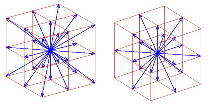
Figure 1: Left: D3Q27 lattice, a three dimensional mesh composed of a set of 27 discrete velocities. Right: D3Q19 lattice, a three dimensional mesh composed of a set of 19 discrete velocities.

To correctly solve the Boltzmann kinetic equation, the set of discrete velocities must be chosen in order to secure enough symmetry to comply with mass-momentum-energy conservation laws of macroscopic hydrodynamics as well as with rotational symmetry. In Fig. 1, two typical 3D lattices used for current LB simulations are shown, one with a set of 27 velocities (D3Q27, left) and the other one with 19 discrete velocities (D3Q19, right).

In its simplest and most compact form, the LB equation reads as follows:

$$f(\vec{x}+\vec{c}_{i},t+1)=f^{\prime}_{i}(\vec{x};t)\equiv(1-\omega)f_{i}(\vec{x};t)+\omega f_{i}^{eq}(\vec{x};t)+S_{i},\;\;i=1,b$$ (1)

where $\vec{x}$ and $\vec{c}_{i}$ are 3D vectors in ordinary space, $f_{i}^{eq}$ are the equilibrium distribution functions and $S_{i}$ is a source term. Such equation represents the following situation: the populations at site $\vec{x}$ at time $t$ collides (a.k.a. collision step) and produce a post-collision state $f^{\prime}_{i}(\vec{x};t)$, which is then scattered away to the corresponding neighbour (a.k.a. propagation step) at $\vec{x}_{i}$ at time $t+1$.

The lattice time step is made unitary, so that $\vec{c}_{i}$ is the length of the link connecting a generic lattice site node $\vec{x}$ to its $b$ neighbors, located at $\vec{x}_{i}=\vec{x}+\vec{c}_{i}$. In the D3Q19 lattice, for example, the index $i$ runs from $1$ to $19$, hence there are $19$ directions of propagation (i.e. neighbors) for each grid-point $\vec{x}$.

The local equilibrium populations are provided by a lattice truncation, to second order in the Mach number $M=u/c_{s}$, of the Maxwell-Boltzmann distribution, namely

$$f_{i}^{eq}(\vec{x};t)=w_{i}\rho(1+u_{i}+q_{i})$$ (2)

where $w_{i}$ is a set of weights normalized to unity, $u_{i}=\frac{\vec{u}\cdot\vec{c}_{i}}{c_{s}^{2}}$ and $q_{i}=(c_{ia}c_{ib}-c_{s}^{2}\delta_{ab})u_{a}u_{b}/2c_{s}^{4}$, with $c_{s}$ equal to the speed of sound in the lattice, and an implied sum over repeated latin indices $a,b=x,y,z$.

The source term $S_{i}$ of Eq. 1 typically accounts for the momentum exchange between the fluid and external (or internal) fields, such as gravity or self-consistent forces describing potential energy interactions within the fluid.

By defining fluid density and velocity as

$$\rho=\sum_{i}f_{i}\hskip 56.9055pt\vec{u}=(\sum_{i}f_{i}\vec{c}_{i})/\rho,$$ (3)

the Navier-Stokes equations for an isothermal quasi-incompressible fluid can be recovered in the continuum limit if the lattice has the suitable symmetries aforementioned and the local equilibria are chosen according to Eq. 2.

Finally, the relaxation parameter $\omega$ in Eq. 1 controls the viscosity of the lattice fluid according to

$$\nu=c_{s}^{2}(\omega^{-1}-1/2).$$ (4)

Further details about the method can be found in Ref. [28, 34].

One of the main strengths of the LB scheme is that, unlike advection, streaming is i) exact, since it occurs along straight lines defined by the lattice velocity vectors $\vec{c}_{i}$, regardless of the complex structure of the fluid flow, and ii) it is implemented via a memory-shift without any floating-point operation. This also allows to handle fairly complex boundary conditions [35] in a more conceptually transparent way with respect to other mesoscale simulation techniques [36].

3.1 Multi-component flows

The LB method successfully extends to the case of multi-component and multi-phase fluids. In a binary fluid, for example, each component (denoted by $r$ and $b$ for red and blue, respectively) comes with its own populations plus a term modeling the interactions between fluids.

In this case the equations of motion read as follows:

$$f^{r}_{i}(\vec{x}+\vec{c}_{i};t+1)=(1-\omega_{eff})f^{r}_{i}(\vec{x};t)+\omega_{eff}f_{i}^{eq,r}(\rho^{r};\vec{u})+S^{r}_{i}(\vec{x};t)$$ (5)

$$f^{b}_{i}(\vec{x}+\vec{c}_{i};t+1)=(1-\omega_{eff})f^{b}_{i}(\vec{x};t)+\omega_{eff}f_{i}^{eq,b}(\rho^{b};\vec{u})+S^{b}_{i}(\vec{x};t)$$ (6)

$$\omega_{eff}=2c_{s}^{2}/(2\bar{\nu}-c_{s}^{2})$$ (7)

$$\frac{1}{\bar{\nu}}=\frac{\rho_{k}}{(\rho_{k}+\rho_{\bar{k}})}\frac{1}{\nu_{k}}+\frac{\rho_{\bar{k}}}{(\rho_{k}+\rho_{\bar{k}})}\frac{1}{\nu_{\bar{k}}}$$ (8)

where $\omega_{eff}$ is related to the kinematic viscosity $\bar{\nu}$ of the mixture of the two fluids.

The extra term $S^{r}_{i}(\vec{x};t)$ of Eq. 5 (and similarly for $S^{b}$) can be computed as the difference between the local equilibrium population, calculated at a shifted fluid velocity, and the one taken at the effective velocity of the mixture [37], namely:

$$S^{r}_{i}(\vec{r};t)=f_{i}^{eq,r}(\rho^{r},\vec{u}+\frac{\vec{F}^{r}\Delta t}{\rho^{r}})-f_{i}^{eq,r}(\rho^{r},\vec{u}).$$ (9)

Here $\vec{F}^{r}$ is an extra cohesive force, usually defined as [38]

$$\vec{F}^{r}(\vec{x},t)=\rho^{r}(\vec{x},t)G_{C}\sum_{i}w_{i}\rho^{b}(\vec{x}+\vec{c}_{i},t)\vec{c_{i}},$$ (10)

capturing the interaction between the two fluid components. In Eq. 10, $G_{C}$ is a parameter tuning the strength of this intercomponent force, and takes positive values for repulsive interactions and negative for attractive ones.

This formalism has proved extremely valuable for the simulation of a broad variety of multiphase and multi-component fluids and represents a major mainstream of current LB research.

4 LB on Exascale class computers

Exascale computers are the next major step in the high performance computing arena, the deployment of the first Exascale class computers being planned at the moment for 2022. To break the barrier of $10^{18}$ floating point operations per second, this class of machines will be based on a hierarchical structure of thousands of nodes, each with up to hundreds cores using many accelerators like GPGPU (General Purpose GPU or similar devices) per node. Indeed, a CPU-only Exascale Computer is not feasible due to heat dissipation constraints, as it would demand more than of 100MW of electric power!

As a reference, the current top-performing Supercomputer (Summit) in 2019 is composed of 4608 nodes, with 44 cores per node and 6 Nvidia V100 GPU per node, falling short of the Exascale target by a factor five, namely 200 Petaflops (see online at Top500, [39]), and over 90% of the computational performance being delivered by the GPUs.

Since no major improvement of single-core clock time is planned, due again to heat power constraints, crucial to achieve exascale performance is the ability to support concurrent execution of many tasks in parallel, from $O(10^{4})$ for hybrid parallelization (e.g. OpenMP+MPI or OpenAcc+MPI) up to $O(10^{7})$ for a pure MPI parallelization.

Hence, three different levels of parallelism have to be implemented for an efficient Exascale simulation: i) at core/floating point unit level: (Instruction level parallelism, vectorization), ii) at node level: (i.e., shared memory parallelization with CPU or CUDA, for GPU, threads), iii) at cluster level: (i.e., distributed memory parallelization among tasks).

All these levels have to be efficiently orcherstrated to achieve performance by the user’s implementations, together with the tools (compilers, libraries) and technology and the topology of the network, as well as the efficiency of the communication software. Not to mention other important issues, like reliability, requiring a fault tolerant simulation environment [40, 41].

How does LB score in this prospective scenario?

In this respect, the main LB features are as follows:

• Streaming step is exact (zero round-off)

• Collision step is completely local (zero communication)

• First-neighbors communication (eventually second for high-order formulations)

• Conceptually easy-to-manage boundary conditions (e.g. porous media)

• Both pressure and fluid stress tensor are locally available in space and time

• Emergent interfaces (no front-tracking) for multi-phase/species simulation

All features above are expected to facilitate exascale implementations [42]. In Ref. [43], an overview of different LB code implementations on a variety of large-scale HPC machines is presented, and it is shown that LB is, as a matter of fact, in a remarkable good position to exploit Exascale systems.

In the following we shall present some figures that can be reached with LB codes on exascale systems.

According to the roofline model [44], achievable performance can be ranked in terms of Operational Intensity (OI), defined as the ratio between flops performed and data that need to be loaded/stored from/to memory. At low OI ($<10$), the performance is limited by the memory bandwidth, while for higher values the limitation comes from the floating point units availability. It is well known that LB is a bandwidth limited numerical scheme, like any other CFD model. Indeed, the OI index for LB schemes is around 0.7 for double precision (DP) simulations using a D3Q19 lattice (see Fig. 2 where the roofline for LB is shown).

In Fig. 3, a 2D snapshot of the vorticity of the flow around a 3D cylinder at $Re=2000$ is shown ([45] in preparation).
This petascale class simulation was performed with an hybrid MPI-OpenMP parallelization (using 128 Tasks and 64 threads per task), using a single-phase, single time relaxation, 3D lattice. Using $O(10^{4})$ present-day GPUs, a hundred billion lattice simulation would complete one million time-steps in something between $1$ and $3$ hours, corresponding to about 3 and 10 TLUPS (1 Tera LUPS is a trillion Lattice Units per Second). So using an Exascale machine more realistic structure, both in terms of size, complexity (i.e. decorated structure) and simulated time can be performed [46]. To achieve this we must be able to handle order of $10^{4}$ tasks, and each of them must be split in many, order of $1^{\prime}000$, GPUS threads-like processes.

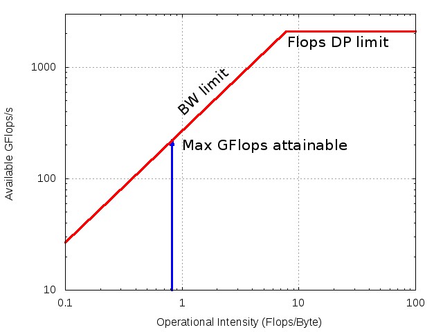
Figure 2: Roofline model for single-phase, single time relaxation, Lattice Boltzmann. The vertical line indicates the performance range using double precision.

Figure 3: Vorticity of a flow around a cylinder at Reynolds number $=2000$. The color map indicates the direction of rotation, blue for clockwise and red for counterclockwise. The flow was simulated with an optimised LB code for macroscopic hydrodynamics [42]

What does this mean in terms of the multiscale problems sketched in the opening of this article?

With a one micron lattice spacing and one nanosecond timestep, this means simulating a cubic box 5 mm in side over one millisecond in time. Although this does not cover the full six orders in space, from, say, 10 nanometers to centimeters, which characterize most meso-materials, it offers nonetheless a very valuable order of magnitude boost in size as compared to current applications.

5 LB method for microfluidic crystals

As mentioned in the Introduction, many soft matter systems host concurrent interactions encompassing six or more decades in space and nearly twice as many in time. Two major directions can be endorsed to face this situation: the first consists in developing sophisticated multiscale methods capable of covering five-six spatial decades through a clever combination of advanced computational techniques, such as local grid-refinement, adaptive grids, or grid-particle combinations [47, 48, 49, 50, 51].

The second avenue consists in developing suitable coarse-grained models, operating at the mesoscale, say microns, through the incorporation of effective forces and potentials designed in such a way as to retain the essential effects of the fine-grain scales on the coarse-grained ones (often providing dramatic computational savings)

Of course, the two strategies are not mutually exclusive; on the contrary, they should be combined in a synergistic fashion, typically employing as much coarse-graining as possible to reduce the need for high-resolution techniques.

In [9], the second strategy has been successfully adopted to the simulation of microdevices. Experiments [7, 8] have shown that a soft flowing microfluidic crystal can be designed by air dispersion in the fluid with a flow focuser: the formation of drops is due to the balance between pressure drop, due to the sudden expansion of the channel, and the shear stress, exerted by the continuous phase inside the nozzle.

In Fig. 4 (top), we show the typical experimental setup for the production of ordered dispersion of mono-disperse air droplets.

Figure 4: (Top). Flow focuser used for the production of air bubbles [7, 8]. Gas is injected from the horizontal branch at pressure $P_{g}$ while air enters at flow rate $Q_{l}/2$ from the two vertical braches. They are focused into a striction of width $\simeq 100$ $\mu$m, and resulting air bubbles are collected downstream in the outlet chamber. (Bottom) Lattice Boltzmann simulation showing the production of roughly mono-disperse fluid droplets within a microfluidic flow focuser. The red phase represents the dispersed fluid (oil) while the black phase the continuous one (water).

In our LB experiments (Fig. 4, bottom), droplet formation is controlled by tuning i) the dispersion-to-continuous flow ratio $\alpha$ (defined as $\alpha=u_{d}/2u_{c}$, where $u_{d}$ and $u_{c}$ are the speeds of the dispersed and the continuous phase at the inlet channel) and by ii) the mesoscopic force $F_{rep}$ modeling the repulsive effect of a surfactant confined at the fluid interface.

The dispersed phase (in red in Fig. 4, bottom) is pumped with a predefined speed $u_{d}$ within the horizontal branch, whereas the continuous phase (black) comes from the two vertical branches at speed $u_{c}$. They are driven into the orifice ,where the droplet form and are finally collected in the outlet chamber. A schematic representation of $F_{rep}$ on the lattice is reported in Fig.5. This term enters the LB equation as a forcing contribution acting solely at the fluid interfaces when in close contact. Its analytical expression is

$$F_{rep}=-A_{h}[h(x)]n\delta_{I},$$ (11)

where $\delta_{I}\propto\nabla\psi$ is a function, proportional to the fluid concentration $\psi$, confining the near-contact force at the fluid interface, while $A_{h}[h(x)]$ sets the strength of the near-contact interactions. It is equal to a positive constant $A$ if $h<h_{min}$ and it decays as $h^{-3}$ if $h>h_{min}$, with $h_{min}=3-4$ lattice units. Although other functional forms of $A[h(x)]$ are certainly possible, this one proves sufficient to capture the effects occurring at the sub-micron scale, such as the stabilization of the fluid film formed between the interfaces and the inhibition of droplet merging.

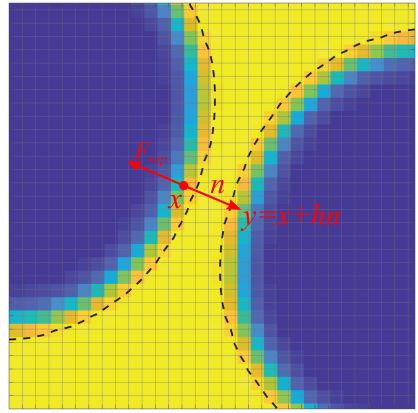
Figure 5: Close-up view of the modelling of the near interaction between two droplets. $F_{rep}$ is the repulsive force and $n$ is the unit vector perpendicular to the interfaces, while $x$ and $y$ indicate the positions, at distance $h$, located within the fluid interface.

An appropriate dimensionless number capturing the competition between surface tension $\sigma$ and the near-contact forces $F_{rep}$ can be defined as $N_{c}=A\Delta{x}/\sigma$, where $\Delta{x}$ is the lattice spacing.

Usually, if $N_{c}\ll 1$, capillary effects dominate and drops merge, whereas if $N_{c}\sim 1$, close contact interactions prevail and droplet fusion is inhibited. A typical arrangement reproducing the latter case is shown in Fig. 4, obtained for $A_{h}=1$ and $N_{c}=0.1$.

These results suggest that satisfactory compliance with experimental results can be achieved by means of suitable coarse-grained models, which offer dramatical computational savings over grid-refinement methods.

However, success or failure of coarse graining must be tested case by case, since approximations which hold for some materials, say dilute microfluidic crystals, may not necessarily apply to other materials, say dense emulsions in which all the droplets are in near-touch with their neighbours. In this respect, significant progress might be possible by resorting to Machine-Learning techniques [52, 53], the idea being of semi-automating the procedure of developing customized coarse-grained models, as detailed in the next section.

5.1 Machine-learning for LB microfluidics

Machine learning has taken modern science and society by storm. Even discounting bombastic claims mostly devoid of scientific value, the fact remains that the idea of automating difficult tasks through the aid of properly trained neural networks may add a new dimension to the space of scientific investigation [54, 55, 56]. For a recent critical review, see for instance [57].

In the following, we portray a prospective machine-assisted procedure to facilitate the computational design of microfluidic devices for soft mesoscale materials. The idea is to “learn” the most suitable coarse-grained expression of the Korteweg tensor, the crucial quantity controlling non-ideal interactions in soft mesoscale materials.

The procedure develops through three basic steps: 1) Generate high-resolution data via direct microscale simulations; 2) Generate coarse-grained data upon projection (averaging) of high-resolution data; 3) Derive the coarse-grained Korteweg tensor using machine learning techniques fed with data from step 2).

The first step consists of performing very high resolution simulations of a microfluidic device, delivering the fluid density $\rho_{f}(\vec{x}_{f},t_{f})$, the flow field $\vec{u}_{f}(\vec{x}_{f},t_{f})$ at each lattice location $\vec{x}_{f}$ and given time instant $t_{f}$ of a fine-grid simulation with $N_{f}$ lattice sites and $M_{f}$ timesteps, for a total of $D_{f}=4N_{f}M_{f}$ degrees of freedom in three spatial dimensions. To be noted that such fine-grain information may be the result of an underlying molecular dynamics simulation.

The second step consists of coarse-graining the high-resolution data to generate the corresponding “exact” coarse-grained data. Upon suitable projection, for instance averaging over blocks of $B=b^{4}$ fine-grain variables, $b$ being the spacetime blocking factor, this provides the corresponding (“exact”) coarse-grained density and velocity $\rho_{c}$ and $\vec{u}_{c}$, for a total of $D_{c}=D_{f}/B\ll D_{f}$ degrees of freedom.

The third step is to devise a suitable model for the Korteweg tensor at the coarse scale $x_{c}=bx_{f}$. A possible procedure is to postulate parametric expressions of the coarse-grained Korteweg tensor, run the coarse grained simulations and perform a systematic search in parameter space, by varying the parameters in such a way as to minimize the departure between the ”exact” expression $K_{c}=\mathcal{P}\rho_{f}$ obtained by projection of the fine-grain simulations and the parametric expression $K_{c}[\rho_{c};\lambda]$, where $\lambda$ denotes the parameters of the coarse-grained model, typically the amplitude and range of the coarse-grained forces.

The optimization problem reads as follows: find $\lambda$ such as to minimise the error,

$$e[\lambda]=\left\lVert(P_{c},P_{c}[\lambda])\right\rVert$$ (12)

where $\left\lVert..\right\rVert$ denotes a suitable metrics in the $D_{c}$-dimensional functional space of solutions.

This is a classical and potentially expensive optimization procedure.

A possible way to reduce its complexity is to leverage the machine learning paradigm by instructing a suitably designed neural network (NN) to “learn” the expression of $K_{c}$ as a functional of the coarse-grained density field $\rho_{c}$. Formally:

$$K_{c}^{ml}=\sigma_{L}[W\rho_{c}]$$ (13)

where $\rho_{c}=\mathcal{P}\rho_{f}$ is the “exact” coarse-grained density and $\sigma_{L}$ denotes the set of activation functions of a $L$-levels deep neural network, with weights $W$.

Note that the left hand side is an array of $6D_{c}$ values, six being the number of independent components of the Korteweg tensor in three dimensions, while the input array $\rho_{c}$ contains only $D_{c}$ entries. Hence, the set of weights in a fully connected NN contains $36N_{c}^{2}$ entries. This looks utterly unfeasible, until one recalls that the Korteweg tensor only involves the Laplacian and gradient product of the density field

$$K_{ab}=\lambda[\rho\Delta\rho+\frac{1}{2}(\nabla\rho)^{2}]\delta_{ab}-\lambda\nabla_{a}\rho\nabla_{b}\rho$$

where $a,b=x,y,z$ and $\lambda$ controls the surface tension.

The coarse-grain tensor is likely to expose additional nonlocal terms, but certainly no global dependence, meaning that the set of weights connecting the value of the $K$-tensor at a given lattice site to the density field should be of the order of O(100) at most.

For the sake of generality, one may wish to express it in integral form

$$K_{c}(\vec{x}_{c})=\rho(\vec{x}_{c})\int G(\vec{x}_{c},\vec{y}_{c})\rho(\vec{y}_{c})d\vec{y}_{c}$$ (14)

and instruct the machine to learn the kernel $G$.

This is still a huge learning task, but not an unfeasible one, the number of parameters being comparable to similar efforts in ab-initio molecular dynamics, whereby the machine learns multi-parameter coarse-grained potentials [58, 59].

Further speed can be gained by postulating the functional expression of the coarse grained $K$-tensor in formal analogy with recent work on turbulence modelling [60], i.e. based on the basic symmetries of the problem, which further constrains the functional dependence of $K_{c}$ on the density field.

Work is currently in progress to implement the aforementioned ideas.

6 High-performance LB code for bijel materials

For purely illustrative puroposes, in this section we discuss a different class of complex flowing systems made up of colloidal particles suspended in a binary fluid mixture, such as oil and water.

A notable example of such materials is offered by bijels [4], soft materials consisting of a pair of bi-continuous fluid domains, frozen into a permanent porous matrix by a densely monolayer of colloidal particles adsorbed onto the fluid-fluid interface.

The mechanical properties of such materials, such as elasticity and pore size, can be fine-tuned through the radius and the volume fraction of the particles, typically in the range $0.01<\phi<0.1$, corresponding to a number

$$N=\frac{3\phi}{4\pi}(\frac{L}{R})^{3}$$

of colloids of radius $R$ in a box of volume $L^{3}$.

Since the key mechanisms for arrested coarsening are i) the sequestration of the colloids around the interface and ii) the replacement of the interface by the colloid itself, the colloidal radius should be significantly larger than the interface width, $R/w>2$. Given that LB is a diffuse-interface method and the interfaces span a few lattice spacings (say three to five), the spatial hierarchy for a typical large scale simulation with, say, one billion grid points reads as follows:

$$dx=1,\;w=3\div 5,\;R=10\div 50,L=1000$$

With a typical volume fraction $\phi=0.1$, these parameters correspond to about $N\sim 10^{3}\div 10^{5}$ colloids.

In order to model bijels, colloidal particles are represented as rigid spheres of radius $R$, moving under the effect of a total force ($\vec{F}_{p}$) and torque ($\vec{T}_{p}$), both acting on the center of mass $\vec{r}_{p}$ of the $p$-th particle.

The particle dynamics obeys Newton’s equations of motion (EOM):

$$\frac{d\vec{r}_{p}}{dt}=\vec{u}_{p},\hskip 14.22636ptm_{p}\frac{d\vec{u}_{p}}{dt}=\vec{F}_{p},\hskip 14.22636ptI_{p}\frac{d\vec{\omega}_{p}}{dt}=\vec{T}_{p},$$ (15)

where $\vec{u}_{p}$ is the particle velocity and $\vec{\omega}_{p}$ is the corresponding angular velocity. The force on each particle takes into account the interactions with the fluid and the inter-particle forces, including the lubrication term [61, 62]. Hence, the equations of motion (EOM) are solved by a leapfrog approach, using quaternion algebra for the rotational component ([63, 64]).

The computation is parallelised using MPI. While for the hydrodynamic part the domain is equally distributed (according to a either 1D, or 2D or 3D domain decomposition), for the particles a complete replication of their physical coordinates (position, velocity, angular velocity) is performed.

More specifically, $\vec{r}_{p}$, $\vec{v}_{p}$ and $\vec{\omega}_{p}$ are allocated and maintained in all MPI tasks, but each MPI task solves EOM only for the particles whose centers of mass lie in its sub-domain, defined by the fluid partition. Whenever a particle crosses two or more sub-domains, the force and torque are computed with an MPI reduction and once the time step is completed, new values of $\vec{r}_{p}$, $\vec{v}_{p}$ and $\vec{\omega}_{p}$ are broadcasted to all tasks.

Even at sizeable volume fractions (such as $\phi=0.2$), the number of particles is of the order of ten-twenty thousands, hence much smaller than the dimension of the simulation box ($L^{3}=1024^{3}$), which is why the “replicated data” strategy ([65, 66]) does not significantly affect the MPI communication time (see Fig.6).

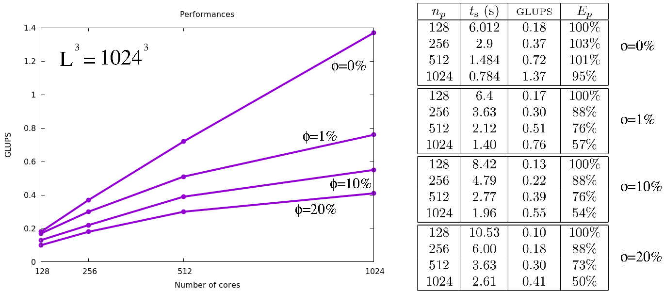
Figure 6: Left: GLUPS versus number of cores measured in a cubic box of linear size $L=1024$, in which spherical colloids are dispersed in a bicontinuous fluid. From the top to the bottom, the box was filled with $N=0$, $N=15407$, $N=154072$, and $N=308144$ colloids, corresponding to a particle volume fraction $\phi$ equal to 0%, 1%, 10% and 20%, respectively. Right: Run (wall-clock) time, in seconds, per single time step iteration, $t_{\text{s}}$, with corresponding GLUPS and parallel efficiency, $E_{p}$, versus the number of computing cores, $n_{p}$ for the same system. Note that the parallel efficiency is reported in percentage.

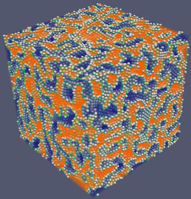
Figure 7: Typical morphology of a bijel material obtained by dispersing rigid colloids (of radius $R=5.5$ lu) in a bicontinuous fluid. Particles are adsorbed at the fluid interface and, if their volume fraction is sufficiently high, domain coarsening arrests. Red and blue colors indicate the two fluid components while grey spheres are colloids.

Results from a typical simulation of a bijel are shown in Fig.7, in which solid particles accumulate at the interface leading to the arrest of the domain coarsening of the bi-continuous fluid, which in turn supports the the formation of a soft and highly porous fluid matrix. Further results are shown in Fig 8, in which the bijel is confined within solid walls with opposite speeds $\pm U=0.01$, hence subject to a shear $S=2U/H$, $H$ being the channel width. The complex and rich rheology of such confined bijels is a completely open research item, which we are currently pursuing through extensive simulations using LBsoft, a open-source software for soft glassy emulsion simulations [67].

Figure 8 reports the bijel before and after applying the shear over half-million timesteps. From this figure, it is apparent that the shear breaks the isotropy of the bijel, leading to a highly directional structure aligned along the shear direction. Further simulations show that upon releasing the shear for another half-million steps does not recover the starting condition, showing evidence of hysteresis.

This suggests the possibility of controlling the final shape of the bijel by properly fine-tuning the magnitude of the applied shear, thereby opening the possibility to exploit the shear to imprint the desired shape to bijels within controlled manufacturing processes.

Systematic work along these lines is currently in progress

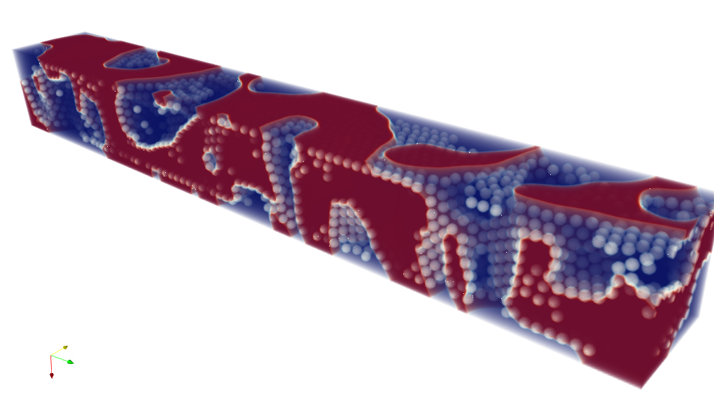
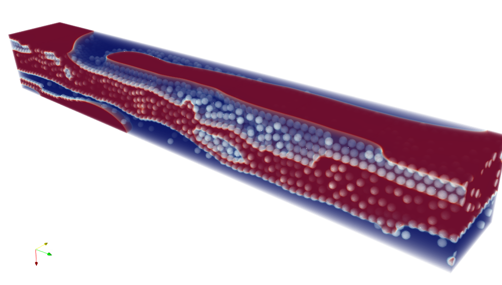
Figure 8: Bijel in a channel of $128\times 128\times 1024$ lu: top and bottom walls slide with opposite directions (aligned with the mainstream axis $z$). Left-right walls are bounce-back while the mainstream axis $z$ is periodic. The main parameters are as follows: wall speed $U=0.01$, volume fraction $\phi=0.15$, sphere radius $R=5.5$ lu. Top: Initial configuration. Bottom: Elongated structures after half-million steps with applied shear.

As to performance, LBsoft delivers GLUPS on one-billion gridpoint configurations on large-scale parallel platforms, with a parallel efficiency ranging from above ninety percent for plain LB (no colloids), down to about fifty percent with twenty percent colloidal volume fractions (see Fig. 6).

Assuming parallel performance can be preserved up to TLUPS, on a Exascale computer, one could run a trillion gridpoint simulation (four decades in space) over one million timesteps in about two weeks wall-clock time.

Setting the lattice spacing at $1$ nm to fully resolve the colloidal diameter ($10-100$ nm), this corresponds to a sample of material of $10$ micron in side, over a time span of about one microsecond.

By leveraging dynamic grid refinement around the interface, both space and time spans could be boosted by two orders of magnitude. However, the programming burden appears fairly significant, especially due to the presence of the colloidal particles.

Work along these lines is also in progress.

7 Summary and outlook

Summarising, we have discussed some of the main challenges and prospects of Exascale LB simulations of soft flowing systems for the design of novel soft mesoscale materials, such as microfluidic crystals and colloidal bijels.

Despite major differences in the basic physics, both systems raise a major challenge to computer modelling, due to the coexistence of dynamic interactions over about six decades in space, from tens of nanometers for near-contact interactions, up to the centimeter scale of the experimental device. Covering six spatial decades by direct numerical simulations is beyond reach even for Exascale computers, which permit to span basically four (a trillion gridpoints). The remaining two decades can either be simulated via local-refinement methods, such as multigrid or grid-particle hybrid formulations, or by coarse-graining, i.e. subgrid modeling of the near-contact interactions acting below the micron scale. Examples of both strategies have been discussed and commented on.

We conclude with two basic takehome’s: 1) Extracting exascale performance from exascale computers requires a concerted multi-parallel approach, no “magic paradigm” is available, 2) even with exascale performance secured, only four spatial decades can be directly simulated, hence many problems in soft matter research will still require an appropriate blend of grid-refinement techniques and coarse-grained models. The optimal combination of such two strategies is most likely problem-dependent, and in some fortunate instances, the latter alone may suffice. However, in general, future generations of computational soft matter scientists should be prepared to imaginative and efficient ways of combining the two.

8 Acknowledgements

S. S., F. B., M. L., A. M. and A. T. acknowledge funding from the European Research Council under the European Union’s Horizon 2020 Framework Programme (No. FP/2014-2020) ERC Grant Agreement No.739964 (COPMAT).

References

- [1] A. Fernandez-Nieves, A. M. Puertas, Fluids, colloids, and soft materials: an introduction to soft matter physics, Wiley Online Library, 2016.
- [2] R. Piazza, Soft matter: the stuff that dreams are made of, Springer Science & Business Media, 2011.
- [3] M. Doi, Soft matter physics, Oxford University Press, 2013.
- [4] K. Stratford, R. Adhikari, I. Pagonabarraga, J.-C. Desplat, M. E. Cates, Colloidal jamming at interfaces: A route to fluid-bicontinuous gels, Science 309 (5744) (2005) 2198–2201.
- [5] S. Frijters, F. Günther, J. Harting, Effects of nanoparticles and surfactant on droplets in shear flow, Soft Matter 8 (24) (2012) 6542–6556.
- [6] M. Costantini, C. Colosi, J. Guzowski, A. Barbetta, J. Jaroszewicz, W. Swieszkowski, M. Dentini, P. Garstecki, Highly ordered and tunable polyhipes by using microfluidics, Journal of Materials Chemistry B 2 (16) (2014) 2290–2300.
- [7] J.-P. Raven, P. Marmottant, Microfluidic crystals: dynamic interplay between rearrangement waves and flow, Physical review letters 102 (8) (2009) 084501.
- [8] P. Marmottant, J.-P. Raven, Microfluidics with foams, Soft Matter 5 (18) (2009) 3385–3388.
- [9] A. Montessori, M. Lauricella, N. Tirelli, S. Succi, Mesoscale modelling of near-contact interactions for complex flowing interfaces, Journal of Fluid Mechanics 872 (2019) 327–347.
- [10] A. Montessori, M. Lauricella, A. Tiribocchi, S. Succi, Modeling pattern formation in soft flowing crystals, Physical Review Fluids 4 (7) (2019) 072201.
- [11] R. Cant, E. Mastorakos, An introduction to turbulent reacting flows, Imperial College Press, 2008.
- [12] G. Muschiolik, E. Dickinson, Double emulsions relevant to food systems: preparation, stability, and applications, Comprehensive Reviews in Food Science and Food Safety 16 (3) (2017) 532–555.
- [13] M. Bernaschi, S. Melchionna, S. Succi, Mesoscopic simulations at the physics-chemistry-biology interface, Reviews of Modern Physics 91 (2) (2019) 025004.
- [14] P. Garstecki, G. M. Whitesides, Flowing crystals: Nonequilibrium structure of foam, Physical review letters 97 (2) (2006) 024503.
- [15] A. Abate, D. Weitz, High-order multiple emulsions formed in poly (dimethylsiloxane) microfluidics, Small 5 (18) (2009) 2030–2032.
- [16] T. Beatus, R. H. Bar-Ziv, T. Tlusty, The physics of 2d microfluidic droplet ensembles, Physics reports 516 (3) (2012) 103–145.
- [17] E. Weinan, Principles of multiscale modeling, Cambridge University Press, 2011.
- [18] M. Levitt, Birth and future of multiscale modeling for macromolecular systems (nobel lecture), Angewandte Chemie International Edition 53 (38) (2014) 10006–10018.
- [19] S. Yip, M. P. Short, Multiscale materials modelling at the mesoscale, Nature materials 12 (9) (2013) 774–777.
- [20] J. Q. Broughton, F. F. Abraham, N. Bernstein, E. Kaxiras, Concurrent coupling of length scales: methodology and application, Physical review B 60 (4) (1999) 2391.
- [21] J. J. De Pablo, Coarse-grained simulations of macromolecules: from dna to nanocomposites, Annual review of physical chemistry 62 (2011) 555–574.
- [22] S. Succi, Lattice boltzmann across scales: from turbulence to dna translocation, The European Physical Journal B 64 (3-4) (2008) 471–479.
- [23] G. Falcucci, S. Ubertini, C. Biscarini, S. Di Francesco, D. Chiappini, S. Palpacelli, A. De Maio, S. Succi, Lattice boltzmann methods for multiphase flow simulations across scales, Communications in Computational Physics 9 (2) (2011) 269–296.
- [24] R. Mezzenga, P. Schurtenberger, A. Burbidge, M. Michel, Understanding foods as soft materials, Nature materials 4 (10) (2005) 729–740.
- [25] G. Gompper, T. Ihle, D. Kroll, R. Winkler, Multi-particle collision dynamics: A particle-based mesoscale simulation approach to the hydrodynamics of complex fluids, in: Advanced computer simulation approaches for soft matter sciences III, Springer, 2009, pp. 1–87.
- [26] H. Noguchi, N. Kikuchi, G. Gompper, Particle-based mesoscale hydrodynamic techniques, EPL (Europhysics Letters) 78 (1) (2007) 10005.
- [27] S. Succi, The lattice Boltzmann equation: for complex states of flowing matter, Oxford University Press, 2018.
- [28] T. Kruger, H. Kusumaatmaja, A. Kuzmin, O. Shardt, G. Silva, E. M. Viggen, The lattice boltzmann method, Springer International Publishing 10 (2017) 978–3.
- [29] A. D´Orazio, S. Succi, Boundary conditions for thermal lattice boltzmann simulations, International Conference on Computational Science (2003) 977–986.
- [30] Z.-G. Feng, E. E. Michaelides, The immersed boundary-lattice boltzmann method for solving fluid–particles interaction problems, Journal of Computational Physics 195 (2) (2004) 602–628.
- [31] M. Praprotnik, L. Delle Site, K. Kremer, Adaptive resolution scheme for efficient hybrid atomistic-mesoscale molecular dynamics simulations of dense liquids, Physical Review E 73 (6) (2006) 066701.
- [32] A. Tiribocchi, F. Bonaccorso, M. Lauricella, S. Melchionna, A. Montessori, S. Succi, Curvature dynamics and long-range effects on fluid–fluid interfaces with colloids, Soft matter 15 (13) (2019) 2848–2862.
- [33] S. Succi, Lattice boltzmann 2038, EPL (Europhysics Letters) 109 (5) (2015) 50001.
- [34] A. Montessori, G. Falcucci, Lattice Boltzmann modeling of complex flows for engineering applications, Morgan & Claypool Publishers, 2018.
- [35] S. Leclaire, A. Parmigiani, O. Malaspinas, B. Chopard, J. Latt, Generalized three-dimensional lattice boltzmann color-gradient method for immiscible two-phase pore-scale imbibition and drainage in porous media, Physical Review E 95 (3) (2017) 033306.
- [36] U. D. Schiller, T. Krüger, O. Henrich, Mesoscopic modelling and simulation of soft matter, Soft matter 14 (1) (2018) 9–26.
- [37] A. Kupershtokh, New method of incorporating a body force term into the lattice boltzmann equation, in: Proc. 5th International EHD Workshop, University of Poitiers, Poitiers, France, 2004, pp. 241–246.
- [38] X. Shan, H. Chen, Lattice boltzmann model for simulating flows with multiple phases and components, Physical review E 47 (3) (1993) 1815.
- [39] TOP500 Supercomputer Sites, https://www.top500.org/ (last accessed April 3, 2020).
- [40] G. Da Costa, T. Fahringer, J. A. R. Gallego, I. Grasso, A. Hristov, H. D. Karatza, A. Lastovetsky, F. Marozzo, D. Petcu, G. L. Stavrinides, et al., Exascale machines require new programming paradigms and runtimes, Supercomputing frontiers and innovations 2 (2) (2015) 6–27.
- [41] M. Snir, R. W. Wisniewski, J. A. Abraham, S. V. Adve, S. Bagchi, P. Balaji, J. Belak, P. Bose, F. Cappello, B. Carlson, et al., Addressing failures in exascale computing, The International Journal of High Performance Computing Applications 28 (2) (2014) 129–173.
- [42] S. Succi, G. Amati, M. Bernaschi, G. Falcucci, M. Lauricella, A. Montessori, Towards exascale lattice boltzmann computing, Computers & Fluids 181 (2019) 107–115.
- [43] Z. Liu, X. Chu, X. Lv, H. Meng, S. Shi, W. Han, J. Xu, H. Fu, G. Yang, Sunwaylb: Enabling extreme-scale lattice boltzmann method based computing fluid dynamics simulations on sunway taihulight, in: 2019 IEEE International Parallel and Distributed Processing Symposium (IPDPS), IEEE, 2019, pp. 557–566.
- [44] S. Williams, A. Waterman, D. Patterson, Roofline: an insightful visual performance model for multicore architectures, Communications of the ACM 52 (4) (2009) 65–76.
- [45] G. Amati, Exascale machine & lattice boltzmann performance (dsfd 2020 conference).
- [46] V. Krastev, G. Amati, S. Succi, G. Falcucci, On the effects of surface corrugation on the hydrodynamic performance of cylindrical rigid structures, The European Physical Journal E 41 (2018) 95.
- [47] M. Mehl, M. Lahnert, Adaptive grid implementation for parallel continuum mechanics methods in particle simulations, The European Physical Journal Special Topics 227 (14) (2019) 1757–1778.
- [48] M. Lahnert, C. Burstedde, C. Holm, M. Mehl, G. Rempfer, F. Weik, Towards lattice-boltzmann on dynamically adaptive grids–minimally-invasive grid exchange in espresso, in: Proceedings of the ECCOMAS Congress, 2016, pp. 1–25.
- [49] D. Lagrava, O. Malaspinas, J. Latt, B. Chopard, Advances in multi-domain lattice boltzmann grid refinement, Journal of Computational Physics 231 (14) (2012) 4808–4822.
- [50] A. Dupuis, B. Chopard, Theory and applications of an alternative lattice boltzmann grid refinement algorithm, Physical Review E 67 (6) (2003) 066707.
- [51] O. Filippova, D. Hänel, Grid refinement for lattice-bgk models, Journal of Computational physics 147 (1) (1998) 219–228.
- [52] Y. LeCun, Y. Bengio, G. Hinton, Deep learning, nature 521 (7553) (2015) 436–444.
- [53] I. Goodfellow, Y. Bengio, A. Courville, Deep learning. vol. 1 (2016).
- [54] G. Carleo, I. Cirac, K. Cranmer, L. Daudet, M. Schuld, N. Tishby, L. Vogt-Maranto, L. Zdeborová, Machine learning and the physical sciences, Reviews of Modern Physics 91 (4) (2019) 045002.
- [55] M. Brenner, J. Eldredge, J. Freund, Perspective on machine learning for advancing fluid mechanics, Physical Review Fluids 4 (10) (2019) 100501.
- [56] Y. Bar-Sinai, S. Hoyer, J. Hickey, M. P. Brenner, Learning data-driven discretizations for partial differential equations, Proceedings of the National Academy of Sciences 116 (31) (2019) 15344–15349.
- [57] S. Succi, P. V. Coveney, Big data: the end of the scientific method?, Philosophical Transactions of the Royal Society A 377 (2142) (2019) 20180145.
- [58] L. Zhang, D.-Y. Lin, H. Wang, R. Car, E. Weinan, Active learning of uniformly accurate interatomic potentials for materials simulation, Physical Review Materials 3 (2) (2019) 023804.
- [59] J. Behler, M. Parrinello, Generalized neural-network representation of high-dimensional potential-energy surfaces, Physical review letters 98 (14) (2007) 146401.
- [60] R. Fang, D. Sondak, P. Protopapas, S. Succi, Neural network models for the anisotropic reynolds stress tensor in turbulent channel flow, Journal of Turbulence (2019) 1–19.
- [61] A. J. Ladd, Numerical simulations of particulate suspensions via a discretized boltzmann equation. part 1. theoretical foundation, Journal of fluid mechanics 271 (1994) 285–309.
- [62] N.-Q. Nguyen, A. Ladd, Lubrication corrections for lattice-boltzmann simulations of particle suspensions, Physical Review E 66 (4) (2002) 046708.
- [63] D. Rozmanov, P. G. Kusalik, Robust rotational-velocity-verlet integration methods, Physical Review E 81 (5) (2010) 056706.
- [64] M. Svanberg, An improved leap-frog rotational algorithm, Molecular physics 92 (6) (1997) 1085–1088.
- [65] W. Smith, Molecular dynamics on hypercube parallel computers, Computer Physics Communications 62 (2-3) (1991) 229–248.
- [66] W. Smith, Molecular dynamics on distributed memory (mimd) parallel computers, Theoretica chimica acta 84 (4-5) (1993) 385–398.
- [67] F. Bonaccorso, A. Montessori, A. Tiribocchi, G. Amati, M. Bernaschi, M. Lauricella, S. Succi, Lbsoft: A parallel open-source software for simulation of colloidal systems, submitted to Computer Physics Communications.