Cavity quantum electro-optics:
Microwave-telecom conversion in the quantum ground state

Abstract

Fiber optic communication is the backbone of our modern information society, offering high bandwidth, low loss, weight, size and cost, as well as an immunity to electromagnetic interference Hecht1999 . Microwave photonics lends these advantages to electronic sensing and communication systems Capmany2007 , but - unlike the field of nonlinear optics - electro-optic devices so far require classical modulation fields whose variance is dominated by electronic or thermal noise rather than quantum fluctuations. Here we present a cavity electro-optic transceiver Matsko2007 ; Tsang2010 ; Tsang2011 ; Rueda2016 ; Javerzac-Galy2016 ; Soltani2017 operating in a millikelvin environment with a mode occupancy as low as $0.025\,\pm 0.005$ noise photons. Our system is based on a lithium niobate whispering gallery mode resonator, resonantly coupled to a superconducting microwave cavity via the Pockels effect Cohen2001 ; Ilchenko2003 ; Fan2018 ; Witmer2020 . For the highest continuous wave pump power of 1.48 mW we demonstrate bidirectional single-sideband conversion of X band microwave to C band telecom light with a total (internal) efficiency of 0.03% (0.7%) and an added output conversion noise of 5.5 photons. The high bandwidth of $10.7\,\text{MHz}$ combined with the observed very slow heating rate of 1.1 noise photons $\text{s}^{-1}$ puts quantum limited pulsed microwave-optics conversion within reach. The presented device is versatile and compatible with superconducting qubits Reed2017 , which might open the way for fast and deterministic entanglement distribution between microwave and optical fields Rueda2019 ; Zhong2020 , for optically mediated remote entanglement of superconducting qubits Kurpiers2018 , and for new multiplexed cryogenic circuit control and readout strategies Ruedacombs ; Youssefi2020 .

The last three decades have witnessed the emergence of a great diversity of controllable quantum systems, and superconducting Josephson circuits are one of the most promising candidates for the realization of scalable quantum processors Arute2019 . However, quantum states encoded in microwave frequency excitations are very sensitive to thermal noise and electromagnetic interference. Short distance quantum networks could be realized with cryo-cooled transmission lines but longer distances and high density networks require coherent upconversion to shorter wavelength information carriers, ideally compatible with existing near infrared (1550 nm) fiber optic technology. So far no solution exists to deterministically interconnect remote quantum microwave systems, such as superconducting qubits Arute2019 and quantum dots or spins in solids Burkard2020 ; Awschalom2018 via a room temperature link with sufficient fidelity to build large-scale quantum networks Kimble2008 . Solving this challenge might not only facilitate a new generation of more power efficient classical communication systems Capmany2007 , but eventually also enable quantum secure communication, modular quantum computing clusters Wehner2018 and powerful quantum sensing networks.

An ideal quantum signal converter Lecocq2016 needs to achieve a total bidirectional conversion efficiency close to unity $\eta\sim 1$ for quantum level signals with a minimum amount of added noise $N\ll 1$ over a large instantaneous bandwidth that allows for fast transduction compared to typical qubit coherence times. Many different platforms are already being explored for microwave to optical photon conversion Lambert2020 ; Lauk2020 . Electro-optomechanical systems have shown very encouraging efficiencies Higginbotham2018 ; Arnold2020 , but typically suffer from a limited bandwidth in the kHz range. Electro-optic Rueda2016 ; Fan2018 ; Witmer2020 or piezo-optomechanical Vainsencher2016 ; Jiang2020 ; Han2020 conversion can be faster but the conversion noise properties have not been quantified. Facilitated by efficient photon counting and low duty cycle operation, unidirectional transduction of quantum level signals has also recently been shown Forsch2020 ; Mirhosseini2020 , but ground state operation has not been demonstrated in a bidirectional interface so far. In this work we present such a device operating continuously with a microwave mode occupancy $N_{\text{e}}\leq 1$, for a pump laser power of up to $P_{p}=23.5\,\mu$W resulting in a total bidirectional conversion efficiency of $\eta_{\text{tot}}=9.1\times 10^{-6}$. The maximum achieved total efficiency of $\eta_{\text{tot}}=0.03\,\%$ is limited by the highest pump laser power of $P_{p}=1.48$ mW for the available setup at millikelvin temperatures.

Theory
Electro-optic converters make use of the nonlinear properties of non-centrosymmetric crystals to couple optical and microwave degrees of freedom. Our resonant transducer has two high quality factor optical modes whose frequency difference matches the resonance frequency of a microwave mode. The system’s interaction Hamiltonian is given as Tsang2010

$$\hat{H}_{\text{int}}=\hbar g(\hat{a}_{e}\hat{a}_{p}\hat{a}_{o}^{\dagger}+\hat{a}_{e}^{\dagger}\hat{a}_{p}^{\dagger}\hat{a}_{o}),$$ (1)

where $\hat{a}_{e}$, $\hat{a}_{p}$, and $\hat{a}_{o}$ stand for the annihilation operators for the microwave, optical pump, and optical signal mode, respectively. This Hamiltonian describes two reciprocal three-wave mixing processes that involve creation and annihilation of photons while respecting energy conservation. The nonlinear vacuum coupling rate $g$ for this interaction depends on the material’s effective electro-optic coefficient $r$ and the spatial overlap of the three modes Rueda2016

$$g=r\,\sqrt{\frac{\varepsilon_{p}\varepsilon_{o}}{\varepsilon_{e}}}\sqrt{\frac{\hbar\omega_{e}\omega_{p}\omega_{o}}{8\varepsilon_{0}V_{e}V_{p}V_{o}}}\int dV\psi_{e}\psi_{p}\psi_{o}^{\star},$$ (2)

with the mode frequency $\omega_{k}$, the relative permittivity $\varepsilon_{k}$ and permeability $\mu_{k}=1$, the effective mode volume $V_{k}$, and the normalized spatial field distribution $\psi_{k}$ defined such that the single-photon electric field for mode $k\in\{e,p,o\}$ can be written as $E_{k}(\vec{r})=\sqrt{\hbar\omega_{k}/(2\varepsilon_{0}\varepsilon_{k}V_{k})}\psi_{k}(\vec{r})$. All three modes are whispering gallery modes (WGM) strekalov2016 whose spatial field distribution can be separated in the cross-sectional and azimuthal part $\psi_{k}(r,z,\phi)=\Psi_{k}(r,z)e^{-im_{k}\phi}$. The integral in Eq. (2) is non-zero only if the azimuthal numbers of the participating modes fulfill $m_{o}=m_{p}+m_{e}$, which is also known as phase matching or angular momentum conservation.

In our conversion scheme we drive the mode $\hat{a}_{p}$ with a bright coherent tone $\hat{a}_{p}\rightarrow\alpha_{p}$, which simplifies Eq. (1) to

$$\hat{H}_{\text{int}}=\hbar\alpha_{p}g(\hat{a}_{e}\hat{a}_{o}^{\dagger}+\hat{a}_{e}^{\dagger}\hat{a}_{o}).$$ (3)

This is known as the beam splitter Hamiltonian and it corresponds to a linear coupling between the optical mode $\hat{a}_{o}$ and microwave mode $\hat{a}_{e}$. From the enhanced coupling rate $\alpha_{p}g$, we define the multi-photon cooperativity as $C=4|\alpha_{p}|^{2}g^{2}/(\kappa_{o}\kappa_{e})$, where $\kappa_{o}$ and $\kappa_{e}$ are the total loss rates of the optical and microwave mode, respectively. The multi-photon cooperativity is the figure of merit in most of the resonant electro-optic devices, both for frequency conversion and entanglement generation Tsang2011 ; Rueda2016 ; Fan2018 ; Rueda2019 .

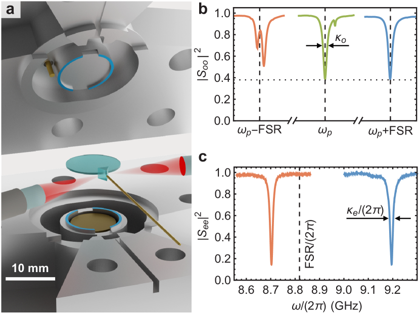
Figure 1: Resonant electro-optic device. a, Exploded-view rendering of the electro-optic converter. The WGM resonator (light blue disc) is clamped between two aluminum rings (blue shaded areas) of the top and bottom part of the aluminum microwave cavity. Two GRIN-lenses are used to focus the optical input and output beams (red) on a diamond prism surface in close proximity of the optical resonator. The microwave tone is coupled in and out of the cavity using a coaxial pin coupler at the top of the cavity (gold). The prism, both lenses and the microwave tuning cylinder (gold shaded inside the lower ring) positions can be adjusted with 8 linear piezo positioners. b, Optical reflection spectrum of the WGM resonator at base temperature ($\sim 7$ mK). The optical pump mode at $\omega_{p}/(2\pi)\approx 193.5$ THz (green) and signal mode (blue) are critically coupled and separated by one free spectral range (FSR, dashed lines). On resonance 38% of the optical power is reflected without entering the WGM resonator due to imperfect optical mode overlap $\Lambda$ (horizontal dotted line). The lower sideband mode (red) was chosen to couple to a mode family of different polarization, which splits it and facilitates the single-sideband selectivity of the converter. c, Reflection spectrum of the microwave cavity at base temperature ($\sim 7$ mK) for the tuning cylinder in its up position (blue line) and in its down position (red line). With a tuning range of $\sim\,0.5$ GHz we can readily match the cavity frequency with that of the optical free spectral range $\text{FSR}/(2\pi)=8.818$ GHz (dashed line).

Device
The electro-optic transducer consists of a z-cut LiNbO₃ WGM resonator, with a major radius $R=2.5$ mm, sidewall surface radius $\rho\approx 0.7$ mm and a thickness $d=0.15$ mm, coupled to a superconducting aluminum cavity as shown in Fig. 1a. The top and bottom rings of the cavity are designed to confine the microwave mode at the rim of the WGM resonator and maximize the spatial mode overlap with the two optical modes. Here we use type-0 frequency conversion, where all the participating waves are polarized parallel to the material’s optic and symmetry axis, addressing the highest electro-optic tensor component of LiNbO₃. We work with two optical modes of the WGM resonator that are spectrally separated by the resonator’s optical free spectral range (FSR) as shown in Fig. 1b. The pump mode has an azimuthal number $m_{p}\approx 20\times 10^{3}$ and the signal mode $m_{o}=m_{p}+1$. The $m_{p}-1$ mode’s participation in the resonant interaction is suppressed due to its avoided crossing with another mode family Rueda2016 , leaving only 2 optical modes in the process. We use an antireflection coated diamond prism to feed the optical pump into the optical resonator via evanescent coupling. The prism is attached to a linear piezo positioning stage that allows to accurately tune the extrinsic optical coupling rate $\kappa_{\text{ex},o}$ in-situ. The continuous wave optical pump is a $\sim 10$ kHz linewidth coherent laser tone that is locked to the resonance of the optical pump WGM at $\omega_{p}/(2\pi)\approx 193.5$ THz for conversion measurements. The cryostat optical input line consists of a single mode fiber with a GRIN-lens at its end to focus the optical beam at the prism-WGM resonator coupling point. The reflected optical pump is collected with a second GRIN-lens and coupled to the output line fiber for further measurements at room temperature.

At base temperature ($\sim 7$ mK) we measure an optical mode separation $\text{FSR}/(2\pi)=8.818$ GHz and an intrinsic optical loss rate $\kappa_{\text{in},o}=9.46$ MHz, which corresponds to a quality factor $Q_{\text{in},o}=2.0\times 10^{7}$ - a reduction by a factor 10 (5) from the measured room temperature value outside (inside) the microwave cavity. The chosen optical pump and signal modes have a contrast of 62% at critical coupling ($Q_{\text{ex},o}=Q_{\text{in},o}$) as shown in Fig. 1b, due to an imperfect spatial field mode overlap $\Lambda^{2}=0.38$ between the optical WGM and the optical input beam (see Supplementary Material). In this work we keep the optical system critically coupled to maximize the optical photon number for a given input power. The optical signal at $\omega_{o}=\omega_{p}+\text{FSR}$ for optical to microwave conversion is created using a suppressed-carrier single-sideband modulator and sent through the same optical path as the pump tone, see Supplementary Information.

The chosen microwave cavity mode undergoes one oscillation around a full azimuthal roundtrip $m_{e}=1$, and its frequency is matched to the optical FSR in order to fulfill the conditions of phase matching and energy conservation. We use an aluminum cylinder centered below the WGM resonator and attached to a vertical piezo positioner that shifts the microwave resonance frequency $\omega_{e}/(2\pi)$ from 8.70 to 9.19 GHz at base temperature as shown in Fig. 1c. Microwave tones are sent to the device through a heavily attenuated transmission line and subsequently coupled to the cavity via a coaxial pin coupler mounted in the top part of the cavity as shown in Fig. 1a. The reflected microwave tone and the down-converted optical signal pass two circulators before amplification and measurement with a vector network analyzer (VNA) or an electronic spectrum analyzer (ESA), see Supplementary Information. From the VNA reflection measurements, we extract the resonance frequency $\omega_{e}$, the intrinsic loss rate $\kappa_{\text{in},e}=6.7$ MHz and the extrinsic coupling rate $\kappa_{\text{ex},e}=3.7$ MHz of the microwave resonance mode.

Bidirectional Conversion
In our system the microwave-to-optics and optics-to-microwave photon conversion efficiencies are equal Tsang2011 . The total input-output electro-optic photon conversion efficiency, defined on resonance, is given as

$$\eta_{\text{tot}}=\eta_{e}\eta_{o}\Lambda^{2}\frac{4C}{(1+C)^{2}},$$ (4)

with coupling efficiencies $\eta_{k}=\kappa_{\text{ex},k}/\kappa_{k}$ and $\kappa_{k}=\kappa_{\text{in},k}+\kappa_{\text{ex},k}$. We determine the bidirectional conversion efficiency of the device $\eta_{\text{tot}}=\sqrt{\eta_{eo}\eta_{oe}}$, independent of the specifics of the measurement setup Andrews2014 , such as the optical and microwave input attenuations $\beta_{1},\beta_{3}$ and output amplifications $\beta_{2},\beta_{4}$ (see Supplementary Material). Performing 4 independent measurements of the coherent scattering parameters $|S_{ij}|^{2}\propto|\hat{a}_{\text{out},i}/\hat{a}_{\text{in},j}|^{2}$ with $i,j=\{e,o\}$ for every optical pump power setting

$$\eta_{\text{tot}}=\sqrt{\frac{|S_{eo}(\omega_{0})|^{2}\cdot|S_{oe}(\omega_{0})|^{2}}{|S_{ee}(\omega_{\Delta})|^{2}\cdot|S_{oo}(\omega_{\Delta})|^{2}}}=\sqrt{\frac{\beta_{1}\eta_{eo}\beta_{4}\cdot\beta_{3}\eta_{oe}\beta_{2}}{\beta_{1}\beta_{2}\cdot\beta_{3}\beta_{4}}},$$ (5)

we obtain the in-situ calibrated device efficiency $\eta_{\text{tot}}$ from the optical fiber to the microwave coaxial line. Here the optics-to-microwave $|S_{eo}|^{2}$ and microwave-to-optics $|S_{oe}|^{2}$ power ratios are measured on resonance $\omega_{0}=\omega_{e},\omega_{o}$ and the reflected optical $|\text{S}_{oo}|^{2}$ and microwave $|\text{S}_{ee}|^{2}$ tones are measured at a detuning such that $|\omega_{\Delta}-\omega_{0}|\gg\kappa_{e},\kappa_{o}$ respectively. For higher accuracy we take into account frequency dependent baseline variations using the full measured reflection scattering parameters.

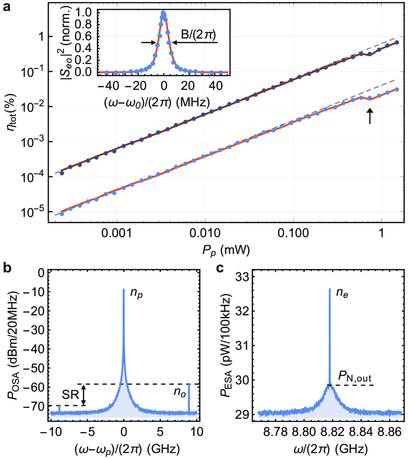
Figure 2: Bidirectional microwave-optics conversion. a, Measured photon conversion efficiency $\eta_{\text{tot}}$ (light blue points) and inferred internal device efficiency $\eta_{\text{int}}=\eta_{\text{tot}}/(\eta_{e}\eta_{o}\Lambda^{2})$ (dark blue points) together with theory (red lines), i.e. Eq. (4) taking into account measured cavity linewidth changes. The dashed lines are linear fits for the 10 lowest power data points respectively. The arrow marks the input power where the aluminum cavity goes from super to normal conducting. The inset shows the measured and normalized coherent optics-to-microwave conversion power ratio for $P_{p}=18.7\,\mu\text{W}$ and $P_{o}=267\,\text{nW}$, as a function of the detuning between the optical signal frequency and $\omega_{o}$ (blue points) together with theory Eq. (6) (red line), indicating the conversion bandwidth $B/(2\pi)=9.0$ MHz. b, Measured optical power spectrum for microwave-to-optical conversion at $P_{p}=1.48\,\text{mW}$. The weak coherent microwave tone $P_{e}=1.0\,\text{nW}$ generates two optical sidebands (blue and red) with a suppression ratio of $SR=10.7$ dB. The center and sideband peaks are proportional to the intra-cavity pump $n_{p}$ and converted optical signal $n_{o}$ photon numbers respectively. The noise floor is set by the resolution bandwidth. c, Measured power spectrum for optical-to-microwave conversion at $P_{p}=2.35\,\mu\text{W}$. The weak optical input signal $P_{o}=161\,\text{nW}$ generates a single coherent microwave tone at $\omega_{o}-\omega_{p}$. In this particular example $n_{e}=1.2$ intra-cavity microwave photons are generated with an incoherent noise floor $P_{N,\text{out}}$ corresponding to an added output conversion noise of $N_{\text{out}}=0.4\,\text{photons}\,\text{s}^{-1}\,\text{Hz}^{-1}$ in the center of the microwave cavity bandwidth.

In Fig. 2a we show the measured values of the total $\eta_{\text{tot}}$ (light blue) and the calculated internal conversion efficiency $\eta_{\text{int}}=\eta_{\text{tot}}/(\eta_{e}\eta_{o}\Lambda^{2})$ (dark blue) together with Eq. (4) taking into account measured cavity linewidth changes (red lines) as a function of the incident optical pump $P_{p}$. As the pump power increases, the conversion efficiency departs only slightly from the expected linear behavior for the low cooperativity limit $(C\ll 1)$ (dashed lines). For $P_{p}\approx$ 700 $\mu$W (arrow), $\eta_{\text{tot}}$ drops because the aluminum cavity undergoes a phase transition from the superconducting to the normal conducting state, which is accompanied by a sudden increase of $\kappa_{\text{in},e}$, see Supplementary Information. The highest conversion efficiency $\eta_{\text{tot}}=3.16\times 10^{-4}$ is reached for the maximum available pump power $P_{p}=1.48$ mW, where the refrigerator base plate reaches a steady state temperature of $T_{f}=320$ mK with theoretical microwave mode occupation of $N_{f}=0.36$.

From the measured values of the bidirectional conversion efficiency $\eta_{\text{tot}}$ and coupling rates $\kappa_{\text{in},e}$ at each optical pump power $P_{p}$, which is related to the drive strength and pump photon number $n_{p}=|\alpha|^{2}=4P_{p}\Lambda^{2}\kappa_{\text{ex},o}/(\hbar\omega_{p}\kappa_{o}^{2})$, we extract the values of the multi-photon cooperativity in the system, ranging from $C=1.23\times 10^{-7}$ for the lowest, to $C=1.67\times 10^{-3}$ for the highest $P_{p}$. From this we deduce the maximum internal photon conversion efficiency $\eta_{\text{int}}=4C/(1+C)^{2}$ of 0.67%. We find very good agreement between the measured conversion efficiency and Eq. (4) (solid red lines) for $g/(2\pi)=40$ Hz, close to the directly measured (simulated) value of 36.1 Hz (36.2 Hz) at room temperature.

The normalized optics-to-microwave conversion as a function of the optical signal frequency is shown in the inset of Fig. 2a. The solid red line corresponds to the theoretical expectation for the conversion spectrum Tsang2011

$$\frac{|\text{S}_{ij}(\omega-\omega_{0})|^{2}}{|\text{S}_{ij}(\omega_{0})|^{2}}=\\ \left(\left(1-\frac{4(\omega-\omega_{0})^{2}}{\kappa_{o}\kappa_{e}}\right)^{2}+\frac{4(\omega-\omega_{0})^{2}(\kappa_{o}+\kappa_{e})^{2}}{\kappa^{2}_{o}\kappa^{2}_{e}}\right)^{-1},$$ (6)

where $\kappa_{e}$ and $\kappa_{o}/(2\pi)=18.92$ MHz were independently extracted from direct reflection measurements. The bandwidth $B/(2\pi)=9.0$ MHz at $P_{p}=18.7\,\mu\text{W}$ with $\kappa_{e}/(2\pi)=11.32$ MHz is in excellent agreement with the theoretical model for both conversion directions (see Supplementary Material). $B/(2\pi)$ increases from 8.51 MHz (calculated, $\kappa_{e}=10.45$ MHz) for the lowest to 10.68 MHz (measured, $\kappa_{e}=14.85$ MHz) for the highest optical pump power.

Selective up-conversion is an important feature of electro-optic transducers, because of the intrinsic noiseless nature of the up-conversion process. Figure 2b displays the measured microwave-to-optics conversion power spectrum corresponding to the highest pump power. Single sideband conversion with a suppression ratio of 10.7 dB in favor of up-conversion can be observed. This is expected from the asymmetric FSR in our WGM resonator due to the splitting of the lower sideband mode as shown in Fig. 1b. The generated microwave output power spectrum from the optics-to-microwave conversion is shown in Fig. 2c, where the peak at the center represents the coherently converted signal power at the microwave cavity output and the broadband incoherent baseline is due to the thermal noise added to the microwave output as a result of optical absorption.

Added noise
The optical pump causes dielectric heating due to absorption in the lithium niobate. In addition, stray light and evanescent fields can lead to direct breaking of Cooper pairs in the superconducting cavity. Both effects cause an increased surface resistance and in turn a larger microwave cavity linewidth $\kappa_{\text{in},e}$ (see Supplementary Information). The optical heating causes an increase of the microwave cavity bath $N_{b}$ and the microwave waveguide bath $N_{\text{wg}}$, both are related to the incoherent microwave mode occupancy Xu2020

$$N_{e}=\eta_{e}N_{\text{wg}}+(1-\eta_{e})N_{b}.$$ (7)

The two bath populations are directly accessible via the detected output noise spectrum given by

$$N_{\text{det}}(\omega)=\frac{4\kappa_{\text{in},e}\kappa_{\text{ex},e}}{\kappa^{2}_{e}+4\omega^{2}}\left(N_{b}-N_{\text{wg}}\right)+N_{\text{wg}}+N_{\text{sys}}$$ (8)

in the low cooperativity limit. The conversion noise at the output port of the device $N_{\text{out}}=N_{\text{det}}-N_{\text{sys}}$ in units of $\text{photons}\,\text{s}^{-1}\,\text{Hz}^{-1}$ is related to the measured power spectrum $P_{\text{ESA}}$ via $N_{\text{det}}(\omega)=P_{\text{ESA}}(\omega)/(\hbar\omega_{e}\beta_{4})$. Here $N_{\text{sys}}=12.74\pm 0.36$ and $\beta_{4}=(67.05\pm 0.16)$ dB are the calibrated noise photon number and gain of the measurement setup as referenced to the converter output port.

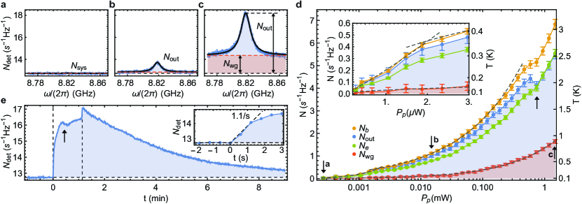
Figure 3: Conversion noise and mode population. a, b, c, Measured microwave output noise spectrum (blue line) in units of $\text{photons}\,\text{s}^{-1}\,\text{Hz}^{-1}$ for (a) $P_{p}=0.23\,\mu$W, (b) 14.82 $\mu$W and (c) 1.48 mW together with a fit to Eq. (8) (black line). In all three panels the dashed black line indicates the measurement system noise floor $N_{\text{sys}}$ and the dashed red line indicates the broad-band noise offset $N_{\text{wg}}$. d, External waveguide bath population $N_{\text{wg}}$ (red), total output noise photons $N_{\text{out}}$ (blue), microwave mode bath $N_{b}$ (yellow) and mode occupancy $N_{e}$ (green) as a function of $P_{p}$. The error bars of $N_{\text{wg}}$ and $N_{\text{out}}$ at low $P_{p}$ are dominated by systematic errors due to slow absolute variations of the baseline of $\pm 0.03$ quanta. The error bars of $N_{b}$ represent the 95% confidence interval of the fit to Eq. (8) which also dominates the uncertainty of $N_{e}$ since $N_{\text{wg}}<N_{\text{b}}$. The error bars at high $P_{p}$ are dominated by the accuracy of the $N_{\text{sys}}$ calibration. The shown error bars are the extrema of these absolute and relative uncertainties. The inset shows the region where the microwave bath occupancy $N_{b}<1$ on a linear scale. The dashed gray lines indicate fitted power laws, specifically $N_{\text{wg}}\propto P_{p}^{0.55}$ over the full range of powers, $N_{\text{b}}\propto P_{p}^{1.14}$ up to $P_{p}\sim 2\,\mu$W (see inset) and $N_{\text{b}}\propto P_{p}^{0.45}$ at higher powers. e, Microwave output noise $N_{\text{out}}$ measured on resonance over a 500 kHz resolution bandwidth in units of $\text{photons}\,\text{s}^{-1}\,\text{Hz}^{-1}$ (blue line) on top of the measurement system noise floor $N_{\text{sys}}$ (dashed horizontal line) as a function of time. The system is excited with a rectangular optical pulse of $P_{p}=1.48\,$mW and a length of 68 seconds (dashed vertical lines). The arrow indicates the time of approximately 30 seconds when superconductivity breaks, the cavity quality factor degrades and the frequency detunes from the measurement frequency. This process is reversed at the end of the pulse when the cavity tunes back and the detected noise increases temporarily. The inset shows the fastest time scale, i.e. the initial heating rate of $dN_{\text{out}}/dt\approx 1.1\,\text{noise photons\, s}^{-1}$.

In Fig. 3a-c we show the measured noise spectrum obtained by normalizing with a no-pump baseline reference measurement when the sample is cold $N_{\text{det}}=N_{\text{sys}}P_{\text{ESA}}/P_{\text{ESA}(P_{p}=0)}$ for three different pump powers with the same y-axis scale and no signal tone applied. For the lowest pump power $P_{p}=0.23\,\mu$W only the $N_{\text{sys}}$ offset is discernible (dashed black lines in panels a-c). For the intermediate power $P_{p}=14.82\,\mu$W the total output microwave noise $N_{\text{out}}=1.01\pm 0.07$ appears as a Lorentzian curve (blue line) with a broad band noise background $N_{\text{wg}}=0.13\pm 0.04$ (red dashed line). For the largest applied power $P_{p}=1.48$ mW we observe a maximum of $N_{\text{out}}=5.51\pm 0.20$ and $N_{\text{wg}}=1.64\pm 0.08$, significantly hotter than the dilution refrigerator base plate at $N_{f}=0.36$. This is expected for a steady-state localized noise source, such as the optically pumped dielectric resonator, which has a finite temperature dependent thermalization rate to equilibrate with the environment.

The added conversion noise referenced to the device output $N_{\text{out}}$ (blue), the broad band waveguide noise $N_{\text{wg}}$ (red), the microwave bath $N_{b}$ (yellow) and mode occupancy $N_{e}$ (green) for different optical pump powers $P_{p}$ are shown in Fig. 3d. Sub-photon microwave output noise as low as $N_{\text{out}}=0.03^{+0.04}_{-0.03}$ and microwave mode occupancies as low as $N_{e}=0.025\pm 0.005$ are achieved for a continuous wave pump power of $P_{p}=0.26\,\mu$W where the total conversion efficiency is $\eta_{\text{tot}}=8.8\times 10^{-8}$.

As the pump power is increased, we observe a smooth growth of the waveguide noise starting from an equivalent temperature of $T_{\text{wg}}=78^{+50}_{-17}$ mK and roughly proportional to $\sqrt{P_{p}}$ over 4 orders of magnitude. This is expected if the effective thermal conductivity to the cold refrigerator bath of approximately constant temperature is increasing linearly such that the heat flow $q$ matches the dissipated part of the pump power $q\propto P_{p}\propto T\cdot\Delta T$, as predicted Woodcraft2005 for normal conducting metals such as the copper coaxial port attached to the superconducting cavity.

In contrast, for the microwave bath we observe 3 distinct regions of heating. Up to about $2\,\mu$W the scaling is approximately linear, which is expected for local heating with a fixed thermalization to the cold bath. The thermal conductivity of superconducting aluminum far below the critical temperature is exponentially suppressed Woodcraft2005 so this thermalization could be due to radiation or direct excitation of quasiparticles. In this important range of noise photon numbers, a high conductivity copper cavity might therefore show a significantly slower trend. Above $2\,\mu$W the scaling is approximately $\sqrt{P_{p}}$, which indicates that part of the cavity, such as the small rings holding the disk, are normal conducting. This is confirmed by an increase in the internal losses (see Supplementary Information). At $P_{p}\approx 0.7$ mW we see a sharp drop in the output noise due to a sudden increase of $\kappa_{\text{in},e}$ from 8.6 to 11.2 MHz. The temporarily slower increase of $N_{b}$ suggests that this is also accompanied by an higher thermalization rate to the cold refrigerator bath, indicating that the entire aluminum cavity undergoes a phase transition at this input power. This interpretation of the data is backed up by stable cavity properties beyond this power (see Supplementary Material). The lowest measured bath occupancies are consistent with qubit measurements for a similar amount of shielding without optics Fink2010 and could be further improved with sensitive radiometry measurements Wang2019 ; Scigliuzzo2020 .

In Fig. 3e we show the time dependence of the measured output noise when the system is excited with a resonant optical square pulse. The measured rise time to the maximum power of $P_{p}=1.48$ mW is 1 ms. Facilitated by its macroscopic device design with a large heat capacity and contact surface area to the cold refrigerator bath, we observe that the fastest timescale at the onset of the square pulse is as low as 1.1 photons s^-1. This is roughly $10^{7}$ times slower compared to state of the art microscopic microwave devices pulsed with $\sim 10^{3}$ times lower power Mirhosseini2020 . Assuming - as a worst case scenario - a linear increase of the heating rate with the applied power, we can project $N_{\text{out}}<10^{-4}$ for a single 100 ns long pulse of power 1 W. For this power $C>1$ with unity internal conversion efficiency and interesting new physics to be unlocked.

Conclusion
The presented bidirectional microwave-optical interface operates in the quantum ground state $N_{e}\ll 1$, as verified by measuring the minimal noise $N_{\text{out}}\ll 1$ added to a converted microwave output signal. Compared to recent probabilistic unidirectional transduction of quantum level signals we showed somewhat lower Mirhosseini2020 and orders of magnitude higher Forsch2020 efficiency. The very high instantaneous bandwidth of $10.7$ MHz compared to typical $100$ Hz repetition rates in previous experiments provides a very promising outlook to be able to also verify the quantum statistics using sensitive heterodyne Rueda2019 or photon detection measurements Zhong2020 in the near future. Furthermore, bandwidth-matched high power pulsed operation schemes should also enable deterministic protocols due to the observed slow heating timescales, i.e. the conversion of quantum level signals with an equivalent input noise $N_{\text{in}}=N_{\text{out}}/\eta_{\text{tot}}\ll 1$. Such a fast and high fidelity quantum microwave photonic interface together with the non-Gaussian resources of superconducting qubits Kurpiers2018 might then provide the practical foundation to extend the range of current fiber optic quantum networks Briegel1998 in analogy to optical-electrical-optical repeaters in the early days of classical fiber optic communication Hecht1999 .

Acknowledgements The authors acknowledge the support from T. Menner, A. Arslani, and T. Asenov from the Miba machine shop for machining the microwave cavity, and S. Barzanjeh, F. Sedlmeir and C. Marquardt for fruitful discussions. This work was supported by IST Austria, the European Research Council under grant agreement number 758053 (ERC StG QUNNECT), and the Austrian Science Fund (FWF) through BeyondC (F71). WH is the recipient of an ISTplus postdoctoral fellowship with funding from the European Union’s Horizon 2020 research and innovation program under the Marie Skłodowska-Curie grant agreement No. 754411. GA is the recipient of a DOC fellowship of the Austrian Academy of Sciences at IST Austria. JMF acknowledges support from the European Union’s Horizon 2020 research and innovation programs under grant agreement No 732894 (FET Proactive HOT), 862644 (FET Open QUARTET), and a NOMIS foundation research grant.
Authors contributions WH, AR, RS, MW and GA worked on the setup and performed the measurements. Data analysis was done by WH, AR and JMF. Analytical modeling and analysis was done by AR and FEM simulations by RS. AR, HGLS and JMF conceived the project. All authors contributed to the manuscript. JMF supervised the project.
Competing interests The authors declare no competing interests.
Data availability The data and code used to produce the results of this manuscript will be made available via an online repository before publication.

Appendix A Measurement setup

The measurement setup used to characterize the performance of the electro-optic converter is shown in Fig. S1.

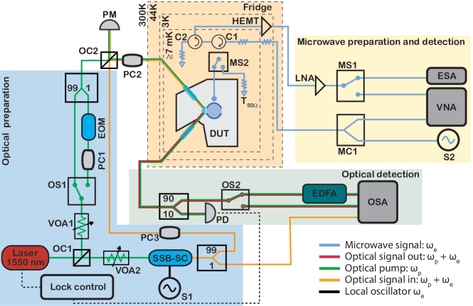
Figure S1: Measurement setup. A tunable laser is equally split (50/50) into two paths at the optical coupler OC1. The upper path is used as the optical pump and it goes through a variable optical attenuator VOA1 that allows to vary $P_{p}$. The optical pump can then be either sent directly to the cryostat fiber, or it can go first through an electro-optic modulator (EOM) in order to create sidebands for spectroscopy calibration. The second path (horizontal) is used to generate the optical signal. It goes also through a variable optical attenuator and it is then frequency up-shifted by $\omega_{e}$ ($\sim$FSR) using a single sideband EO-modulator with suppressed carrier (SSB-SC) driven by a microwave source with local oscillator frequency $\omega_{e}$ (S1). A small fraction (1%) of this signal is picked up and sent directly to an optical spectrum analyzer (OSA) for sideband and carrier suppression ratio monitoring. The rest (99%) is recombined with the pump at OC2, sent to the fridge input fiber and the total power is monitored with a power meter (PM). The optical tones are focused on the prism with a GRIN-lens which then feeds the WGM resonator via evanescent coupling. Polarization controllers PC2 and PC3 are set to achieve maximum coupling to a TE polarized cavity mode. The reflected (or created) optical sideband signal and the reflected pump are collected with the second GRIN-lens and coupled to the cryostat output fiber. The optical signal is then split: 90% of the power goes to the OSA and 10% is sent to a photodiode (PD), which is used for mode spectroscopy and to lock on the optical mode resonance during the conversion measurement. The 90% arm is either sent directly to the OSA, or goes through an EDFA for amplification, depending on the microwave to optics converted signal power. On the microwave side, the signal is sent from the microwave source S2 (or from the VNA for microwave mode spectroscopy) to the fridge input line via the microwave combiner (MC1). The input line is attenuated with attenuators distributed between 3 K and 10 mK with a total of 60 dB in order to suppress room temperature microwave noise. Circulator C1 redirects the reflected tone from the cavity to the amplified output line, while C2 redirects noise coming in from the output line to a matched 50$\Omega$ termination. The output line is amplified at 3 K by a HEMT-amplifier and then at room temperature again with a low noise amplifier (LNA). The output line is connected to switch MS1, to select between an ESA or a VNA measurement. Lastly, microwave switch MS2 allows to swap the device under test (DUT) for a temperature $T_{\text{50}\Omega}$ controllable load, which serves as a broad band noise source in order to calibrate the output line’s total gain and added noise (see D.2)

Appendix B Optical resonator

B.1 WGM resonator fabrication

The whispering gallery mode (WGM) resonator was manufactured from a z-cut congruent undoped lithium niobate wafer. The resonator initial dimensions were a major radius of $R=2.5$ mm, a curvature radius of $\rho\approx 0.7$ mm and an initial thickness $d=$0.5\text{\,}\mathrm{m}\mathrm{m}$$. The lateral surface was polished with diamond slurry from 9 $\mu$m (rms particle diameter) down to 1 $\mu$m. Subsequently, the resonator was thinned down to a 0.15 mm thickness with 5 $\mu$m diamond slurry in a lapping machine. Top and bottom surfaces were then finished by chemical-mechanical polishing.

B.2 Optical prism coupling

We couple the optical pump into the resonator via frustrated total internal reflection between the prism and the resonator surface. The optical beam coming from the cryostat input optical fiber is focused to the coupling window with an angle $\Phi_{c}\approx 50^{\circ}$ using a gradient index (GRIN) lens (see Fig. 1a). The reflected pump and the converted optical signal are caught by a second GRIN lens and directed to the the cryostat output optical fiber. The diamond prism is an isosceles triangle with basis angle 53^∘ and height 0.8 mm. The prism’s input and output sides are anti-reflexion coated, and it is fixed from the backside to a copper wire as shown in Fig. 1a. The copper wire goes through a small canal outside the microwave cavity and is attached to a linear piezo-positioning stage (PS). This way the distance $d$ between the WGM resonator and the prism coupling surface can be controlled with nanometer scale precision.

In order to reduce GRIN lens misalignments during cool down, we machine a single piece, oxygen-free copper holder which has the prism-WGM resonator coupling point at its center. Furthermore, we set up a low temperature realignment system which consists of two ANPx101-LT and one ANPz101-LT PSs from attocube for each GRIN lens, allowing us to align them in the x-y-z direction. A feedback algorithm tracks the overall optical transmission as well as the optical mode contrast during the dilution refrigerator cooldown to 3 K where the final alignments are performed before condensation and further cooldown to the cryogenic base temperature of about 7 mK.

B.3 Optical characterization

The optical resonator is characterized by analyzing its reflection spectrum. We sweep the frequency $\omega/(2\pi)$ of an optical tone over several GHz around 1550 nm and measure the intensity of the reflected signal on a photodiode (PD in Fig. S1). In Fig. S2a we show the pump mode spectrum for a TE polarized tone, whose polarization is parallel to the WGM resonator’s symmetry and optical axis. The optical free spectral range (FSR) for this mode was measured by superimposing it with EOM-generated sidebands from modes one FSR away Rueda2016 (see Fig. S1 for the EOM). The measured optical FSR changed from 8.79 GHz at room temperature to 8.82 GHz at base temperature.

To characterize the coupling to the optical system, we measure the optical mode spectrum for different positions of the prism, thus changing $\kappa_{\text{ex},o}$. The normalized spectrum of the chosen mode follows the analytical model RuedaSanchez2018

$$\frac{|\text{S}_{oo}(\omega-\omega_{o})|^{2}}{|\text{S}_{oo}(\Delta\omega)|^{2}}=1-\frac{4\kappa_{\text{ex},o}\Lambda^{2}(\kappa_{o}-\Lambda^{2}\kappa_{\text{ex},o})}{\kappa^{2}_{o}+4(\omega-\omega_{o})^{2}},$$ (9)

where the factor $\Lambda$ describes the electric field overlap between the evanescent tail of the beam reflecting on the prism and the resonator mode and $\Delta\omega\gg\kappa_{o}$. The external coupling rate $\kappa_{\text{ex},o}$ strongly depends on the distance $d$ between the prism and the resonator

$$\kappa_{\text{ex},o}(d)=\kappa_{\text{ex},o}^{\text{max}}\cdot\exp(-k_{0}\cdot d)$$ (10)

with $\kappa_{\text{ex},o}^{\text{max}}=\kappa_{\text{ex},o}(d=0)$ and $k_{0}=\omega_{o}\sqrt{n^{2}_{\text{LN}}-1}/c$ RuedaSanchez2018 , $n_{\text{LN}}$ the refractive index of LN and $c$ the speed of light in vacuum. We control the distance by applying a DC-voltage to the piezo stage $d\propto-V_{\text{dc}}$ and measure the transmission spectrum. The fitted total optical linewidth $\kappa_{o}=\kappa_{\text{ex},o}+\kappa_{\text{in},o}$ as a function of $V_{\text{dc}}$ is shown in Fig. S2a. From an exponential fit of the measured $\kappa_{o}$ (red line), we extract the offset corresponding to $\kappa_{\text{in},o}/(2\pi)=9.46$ MHz. Furthermore, at critical coupling ($\kappa_{\text{ex},o}=\kappa_{\text{in},o}$), we extract $\Lambda^{2}=0.38$ from a fit to Eq. (9) as shown in Fig. S2a. The intra-cavity photon number for the optical pump is given by

$$n_{p}(\omega)=\frac{P_{p}\Lambda^{2}}{\hbar\omega_{p}}\cdot\frac{4\kappa_{\text{ex},o}}{\kappa_{o}^{2}+4(\omega-\omega_{p})^{2}},$$ (11)

where $P_{p}$ stands for the optical pump power sent to the resonator-prism interface. The WGM resonators’s FSR and linewidth do not change over the full optical pump power range.

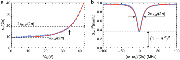
Figure S2: Optical coupling. a, Measured $\kappa_{o}/(2\pi)$ as a function of piezo Voltage $V_{\text{dc}}$ (blue points) and exponential fit (red line). For large distances $d\propto-V_{\text{dc}}$ we find $\kappa_{o}/(2\pi)=\kappa_{\text{in},o}/(2\pi)=9.46$ MHz. The lower dashed line indicates the lower limit $\kappa_{o}=\kappa_{\text{in},o}$. The upper dashed line shows the critical coupling condition where $\kappa_{\text{in},o}=\kappa_{\text{ex},o}$ and $\kappa_{o}=2\kappa_{\text{in},o}$ with the corresponding $V_{\text{dc}}$ (vertical arrow). b, Measured optical reflection spectrum around 1550 nm at base temperature for critical coupling (arrow in panel a). Due to imperfect optical mode matching quantified by $\Lambda^{2}=0.38$ an amount proportional to $(1-\Lambda^{2})^{2}$ of the input power is reflected at critical coupling (dashed line).

Appendix C Microwave cavity

C.1 Design

The conversion efficiency between the optical and microwave modes depends strongly on the microwave electric field confinement at the rim of the WGM resonator. Our hybrid system, based on a 3D-microwave cavity and a WGM resonator, offers a high degree of freedom to control the microwave spatial distribution $\psi_{e}(\vec{r})$, microwave resonance frequency $\omega_{e}$ and external coupling rate $\kappa_{\text{ex},e}$. We used finite element method (FEM) simulations in order to find suitable design parameters for the microwave cavity.

A schematic drawing of the microwave cavity with its important dimensions is shown in Fig. S3a. The LiNbO₃ WGM resonator is clamped between two aluminum rings (highlighted in blue). In this way we maximize the microwave electric field overlap with the optical mode, the latter being confined close to the rim of the WGM resonator (see Fig. S3b). The microwave spatial electric field distribution shows one full oscillation along the circumference of the WGM resonator (see Fig. S3c and d) to fulfill the phase matching condition. The aluminum rings have a cut in the middle in order to maximize the field participation factor and minimize potential magnetic losses in the dielectric. The cavity’s cylindrical inner volume can be tailored to achieve the desired microwave resonance frequency, which can then be tuned by $\sim 500$ MHz in situ, by moving an aluminum cylinder placed inside the lower ring. This allows to compensate the thermal contraction induced frequency shift that occurs during cooldown of the device. The top right part of the shown top half of the cavity is cut out in order to facilitate the assembly of the device.

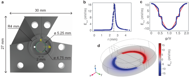
Figure S3: Microwave cavity design. a, Computer aided design drawing of the top part of the aluminum microwave cavity. b, FEM simulation of the single photon electric field distribution of the $m=1$ mode of the microwave cavity. Shown is the z direction of the field along the radial axis at $z=0$ (in the center of the WGM) and $\phi=0$ (yellow dashed line in panel a). The horizontal dashed line marks the position of the edge of the WGM resonator. c, FEM simulation of the z component of the single photon electric field taken at the position of the optical mode maximum and plotted as a function of the azimuthal angle $\phi$ (yellow dashed circle in panel a). The red line is a sinusoidal function as a guide to the eye. d, FEM simulation of the z component of the single photon electric field in the $z=0$ plane of the $m=1$ microwave resonance.

C.2 FEM simulation of electro-optic coupling

From FEM simulations we obtain the single photon spatial electric field distribution given as $E_{e,z}(r,z,\phi)=E_{e,z}^{\text{max}}\Psi_{e}(r,z)(1+f(\phi))\cos(\phi)$, where $\Psi_{e}(r,z)$ is normalized to 1, $r=\sqrt{x^{2}+y^{2}}$ and $\phi=\text{arctan(y/x)}$, see also Fig S3d. For this simulation we used the reported wong2002properties dielectric permittivity of lithium niobate at 9 GHz, i.e. $\varepsilon_{e}={(42.5,42.5,26)}$. The function $f(\phi)$ is symmetric and describes the deviation of the azimuthal field distribution from a pure sinusoidal shape as shown in Fig. S3c. The optical mode is distributed along the ring $\{r=r_{o},\;z=0,\;\phi\in[0\;2\pi]\}$ and the maximum value of the microwave electric field on this ring is $E_{eo}=E_{e,z}(r_{o},0,\phi_{\text{max}})=E_{e,z}^{\text{max}}\Psi_{e}(r_{o},0)=11.1$ mV/m. The optical mode being a clockwise (C) traveling wave, we must decompose the stationary microwave field into a clockwise and a counterclockwise (CC) traveling wave in order to calculate the coupling

$$E_{e,z}(r_{o},0,\phi,t) = E_{eo}(1+f(\phi))\cos(\phi)\cos(\omega_{e}t)$$ (12)

$$= E_{eo}(1+f(\phi))\left(\frac{e^{-i(\phi-\omega_{e}t)}+e^{i(\phi-\omega_{e}t)}+e^{-i(\phi+\omega_{e}t)}+e^{i(\phi+\omega_{e}t)}}{4}\right)$$

$$= E^{+}_{\text{C}}+E_{\text{C}}^{-}+E^{+}_{\text{CC}}+E^{-}_{\text{CC}}.$$

By introducing $E_{e,z}(r_{o},0,\phi,t)$ into Eq. (2), we get ($E^{+}_{\text{CC}}$ and $E^{-}_{\text{CC}}$ do not participate in the interaction)

$$g=n_{p}n_{o}r\sqrt{\frac{\omega_{p}\omega_{o}}{4V_{o}V_{p}}}\frac{E_{eo}}{4}\int dV(\psi_{o}^{*}\psi_{p}e^{-i\phi}+\psi_{o}^{*}\psi_{p}e^{-i\phi}f(\phi)).$$ (13)

Where $n_{p}$ and $n_{o}$ are the refractive indices of the pump $\omega_{p}$ and the sideband $\omega_{o}$. The effective mode volumes $V_{k}$ are given by the integral $\int\text{d}V\psi_{k}\psi_{k}^{*}$ over the respective optical field spatial distributions $\psi_{p}=\Psi_{p}(r,\theta)e^{-im}$ and $\psi_{o}=\Psi_{o}(r,\theta)e^{-i(m+1)}$. The second term in the integral in Eq. (13) is zero due to the symmetry of $f(\phi)$, reducing Eq. (13) to

$$g=\frac{1}{8}\ n_{p}^{2}\omega_{o}r_{33}E_{eo}$$ (14)

where $n_{o}\approx n_{p}=2.13$ ($\varepsilon_{o}\approx\varepsilon_{p}=4.54$) is the extra-ordinary refractive index (dielectric permittivity) of LN at $\omega_{o}\approx\omega_{p}=(2\pi)\times 193.5$ THz and $r_{33}=31$ pm/V is the electro-optic coefficient. For these values we estimate $g_{\text{sim}}/(2\pi)=38$ Hz at room temperature.

C.3 Room temperature measurement of $g$

The system was assembled at room temperature and a microwave tone was fed into the cavity with a coaxial probe coupler of length 1.2 mm. By displacing the tuning cylinder the cavity frequency $\omega_{e}/(2\pi)$ could be shifted from 8.40 to 9.22 GHz, slightly shifted up compared to numerical simulations. We attribute this to small air gaps between the WGM resonator and the aluminum disk, which decrease the effective dielectric constant between the electrodes. To match the measured frequency range exactly, we introduce an air gap of only $\sim$ 1 $\mu$m in the simulations, bringing down the estimated coupling to $g_{\text{sim}}/(2\pi)=36.2$ Hz,

At $\omega_{e}=\text{FSR}$, the microwave mode has the parameters $\kappa_{\text{ex},e}/(2\pi)=2.48$ MHz and $\kappa_{\text{in},e}/(2\pi)=29$ MHz. We infer the nonlinear coupling constant of the system by applying a strong microwave drive tone to the cavity and measuring the resulting optical mode splitting $S\approx 4\sqrt{n_{e}}g_{\text{rt}}$ as described in Ref. Ruedacombs . In Fig. S4a we show a measured splitting of $S/(2\pi)=220$ MHz for a 9.3 dBm microwave pump power applied on resonance. This corresponds to $g_{\text{rt}}/(2\pi)=36.1$ Hz, a five fold improvement compared to earlier results Rueda2016 , and in excellent agreement with the simulations.

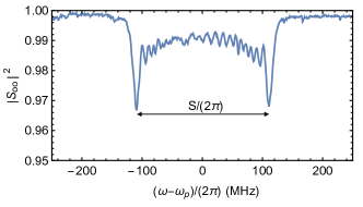
Figure S4: Direct measurement of $g$. Measured optical mode splitting of $S/(2\pi)=220$ MHz at room temperature, obtained with an input power of 9.3 dBm applied to the microwave cavity at $\omega_{e}$. $S\approx 4\sqrt{n_{e}}g_{\text{rt}}$ is related to the measured single photon coupling strength $g_{\text{rt}}/(2\pi)=36.1$ Hz via the calculated intra-cavity photon number $n_{e}=2.3\times 10^{12}$ Ruedacombs .

C.4 Microwave cavity fabrication

The microwave cavity is milled out of a block of pure aluminum (5N). It is divided into a lower and upper part, that are closed after placing the WGM resonator and the prism using brass screws. The internal geometry can be seen in Fig. S3a. When closing the cavity the pure aluminum rings get in contact with the optical resonator. The rings deform slightly, which minimizes the formation of air gaps that would otherwise reduce $g$.

C.5 Microwave characterization

The microwave resonance tuning range was measured with a VNA connected to the cryostat transmission line as shown in Fig. S1. The resonance frequency can be tuned from 8.70 GHz to 9.19 GHz as shown in the main text. This range is at slightly higher frequency compared to the room temperature one. This we attribute to thermal contraction that leads to small air gaps. The decay rates of the microwave mode at the cryogenic base temperature and the lowest optical input power are $\kappa_{\text{ex},e}/(2\pi)=3.7$ MHz and $\kappa_{\text{in},e}/(2\pi)=6.7$ MHz.

Unlike the optical system, the microwave cavity’s parameters undergo changes as a function of the optical pump power $P_{p}$ applied to the WGM resonator. In Fig. S5a we show the normalized spectra of the microwave resonance at the smallest (blue) and largest (red) optical pump power together with a Lorentzian fit. From these measurements we extract the microwave resonance frequency $\omega_{e}$ (shown in panel b) and the internal and external loss rates $\kappa_{\text{in,ex},e}$ (shown in panel c) as function of $P_{p}$. $\kappa_{\text{ex},e}$ depends only on the fixed geometry and is approximately constant. In contrast $\kappa_{\text{in},e}$ increases and $\omega_{e}$ decreases with increasing $P_{p}$ until the microwave cavity undergoes the superconducting phase transition. Once the normal conducting state is reached, a further increase of $P_{p}$ does not lead to any perceptible change, as can be seen in Fig. S5 panels b and c. The microwave resonance red shift (see Fig. S5c) and the $\kappa_{\text{in},e}$ increase are expected due to optically induced creation of quasiparticles in the aluminum cavity as discussed for example in Ref. Witmer2020 . While the local heating is significant, the temperature of the mixing chamber plate of the dilution refrigerator follows a slow ($P_{p}^{0.48}$ at intermediate powers) rise from $T_{f}=7$ mK up to $T_{f}=320$ mK as shown in Fig. S5d.

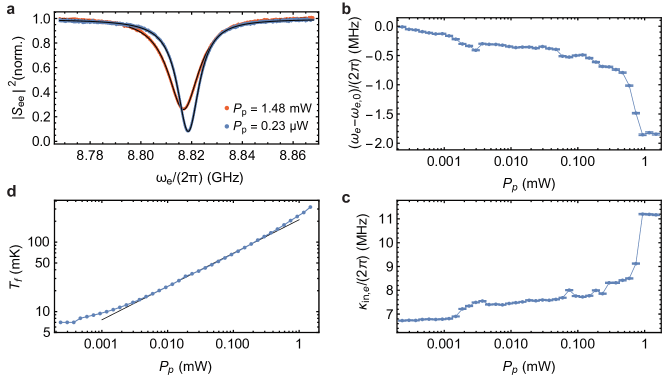
Figure S5: Microwave cavity properties. a, Measured reflection spectra of the microwave resonance for the minimum (blue), and maximum (red) applied optical pump power $P_{p}$ together with Lorentzian fits (black lines). b, Fitted microwave resonance frequency $\omega_{e}-\omega_{e,0}$ as a function of $P_{p}$ with the error bars indicating the 95% confidence interval of the fit. $\omega_{e,0}$ is the fitted resonance frequency obtained for the minimum optical pump power of $P_{p}=0.23\,\mu$W. c, Fitted microwave intrinsic loss rate $\kappa_{\text{in},e}$ as a function of $P_{p}$ with the error bars indicating the 95% confidence interval of the fit. d, The mixing chamber temperature sensor reading $T_{f}$ of the dilution refrigerator as a function of the optical pump power $P_{p}$ (blue points) and a power law fit $T_{f}\propto P_{p}^{0.48}$ to the intermediate power range (black line).

Appendix D Frequency conversion

D.1 Theoretical model

We model the input-output response of the electro-optic system by taking into account external coupling rates $\kappa_{\text{ex},i}$ and internal loss rates $\kappa_{\text{in},i}$ to the external and internal thermal baths, as shown in Fig. S6a. First, we define the coherent conversion matrix as the ratio between the output and the input photon numbers in the absence of noise

$$\eta_{ij}=n_{\text{out},i}/n_{\text{in},j},$$ (15)

for $i,j\in\{o,e\}$. The matrix $\eta_{ij}$ is derived in Ref. Tsang2011 ; RuedaSanchez2018 and its explicit form is given as

$$\left[\begin{array}[]{c}n_{\text{out},o}(\omega)\\ n_{\text{out},e}(\omega)\end{array}\right]=M(\omega)\begin{bmatrix}|(i\omega+\Lambda^{2}\kappa_{\text{ex},o}-\kappa_{o}/2)(\kappa_{e}/2-i\omega)+|G|^{2}|^{2}&\Lambda^{2}\kappa_{\text{ex},e}\kappa_{\text{ex},o}|G|^{2}\\ \kappa_{\text{ex},e}\kappa_{\text{ex},o}|G|^{2}\Lambda^{2}&|(i\omega+\kappa_{\text{ex},e}-\kappa_{e}/2)(\kappa_{o}/2-i\omega)+|G|^{2}|^{2}\end{bmatrix}\times\left[\begin{array}[]{c}n_{\text{in},o}(\omega)\\ n_{\text{in},e}(\omega)\end{array}\right],$$ (16)

where $M^{-1}(\omega)=|(-i\omega+\kappa_{o}/2)(-i\omega+\kappa_{e}/2)+|G|^{2}|^{2}$ and $G=\sqrt{n_{p}}g$, with $n_{p}$ given by Eq. (11).

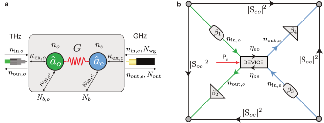
Figure S6: Electro-optic photon conversion. a, Schematic representation of the microwave $(\hat{a}_{e})$ and optical $(\hat{a}_{o})$ modes with coherent populations $n_{e}$ and $n_{o}$ and incoherent occupancies $N_{e}$ and $N_{o}$ (not shown). The electro-optic coupling strength $G=\sqrt{n_{p}}g$ originates from the Pockels effect in the lithium niobate WGM resonator. Both modes are coupled to an internal thermal bath $N_{b}$ and $N_{b,o}$ with the rates $\kappa_{\text{in},i}$. They are also coupled the respective coaxial and fiber waveguides with the rates $\kappa_{\text{ex},i}$. At finite temperature the microwave waveguide has a thermal bath occupancy $N_{\text{wg}}$ and also hosts the total output noise $N_{\text{out}}$ measured in the experiment. b, The $\text{S}_{ij}$ coefficients are defined between the microwave and optical input and output ports outside the cryostat (gray circles). Attenuation for the optical input and output path are $\beta_{1}=-4.81$ dB and $\beta_{2}=-5.5$ dB (without EFDA), or the gain $\beta_{2}=+30.8$ dB (with EFDA). An observed gain saturation at high pump powers is measured and corrected. Attenuation and gain of the microwave input and output path are $\beta_{3}=-74.92$dB and $\beta_{4}=+67.05$dB, respectively. From two conversion measurements on resonance ($S_{ij}$) and two reflection measurements out of resonance ($S_{ii}$) where $\eta_{ii}=1$, we infer the bidirectional photon conversion efficiency of the device according to Eq. (5) and referenced to the input and output photon numbers $n_{\text{in},i}$ and $n_{\text{out},i}$.

The noise performance is one of the most important characteristics of a quantum converter. In our system, we consider two noise sources that affect the microwave mode. The first one is the noise in the waveguide $N_{\text{wg}}$, which can be seen as the external bath of the 50 $\Omega$ semirigid copper coaxial port. The second noise source is given by the internal bath of the system $N_{b}$ as shown in Fig. S6a. The optical waveguide noise $N_{\text{wg},o}$ in the fiber and the internal optical bath noise $N_{b,o}$ are neglected, because $\hbar\omega_{o}\ggg k_{B}T$. In the low cooperativity limit we also neglect the thermal occupancy of the optical mode $N_{o}$, which would give rise to optical output noise $N_{\text{out},o}$.

We define the noise conversion matrix $\sigma_{ij}$ as the ratio between the output noises and the microwave input noise to the system in the absence of any coherent signal as Tsang2011 ; RuedaSanchez2018

$$\left[\begin{array}[]{c}N_{\text{out},o}(\omega)\\ N_{\text{out}}(\omega)\end{array}\right]=M(\omega)\begin{bmatrix}\kappa_{\text{ex},e}\kappa_{\text{ex},o}|G|^{2}&\kappa_{\text{in},e}\kappa_{\text{ex},o}|G|^{2}\\ |(i\omega+\kappa_{\text{ex},e}-\kappa_{e}/2)(-i\omega+\kappa_{o}/2)+|G|^{2}|^{2}&\kappa_{\text{in},e}\kappa_{\text{ex},e}|(-i\omega+\kappa_{o}/2)|^{2}\end{bmatrix}\times\left[\begin{array}[]{c}N_{\text{wg}}(\omega)\\ N_{b}(\omega)\end{array}\right],$$ (17)

where $N_{\text{wg}}(\omega)=(\exp(\hbar\omega/k_{B}T_{\text{wg}})-1)^{-1}$ and $N_{b}(\omega)=(\exp(\hbar\omega/k_{B}T_{\text{b}})-1)^{-1}$ are wide band distributions compared to $\kappa_{\text{ex},e}$, such that they can be approximated as constant.

The full input-output model including vacuum noise is given as

$$\textbf{n}_{\text{out}}(\omega)+\textbf{N}_{\text{out}}(\omega)=\eta_{ij}(\omega)\cdot\textbf{n}_{\text{in}}(\omega)+\sigma_{ij}(\omega)\cdot\textbf{N}_{\{\text{wg},b\}}(\omega)+\textbf{n}_{\text{vac}}.$$ (18)

with $\textbf{n}_{\text{vac}}=\left[\begin{array}[]{c}0.5\\ 0.5\end{array}\right]$.

The device is fixed to the mixing chamber of a dilution refrigerator with a base temperature of $\sim$ 7mK, preventing direct access to the device’s input and output ports, see Fig. S1. In Fig. S6b we present a simplified schematic of the measurement setup, with attenuation and gain $\beta_{1}$, $\beta_{2}$ for the optical path, and $\beta_{3}$, $\beta_{4}$ for the microwave path. We define the measured scattering matrix including the transmission lines on resonance as

$$|\text{S}_{ij}(\omega_{0})|^{2}=\frac{1}{(1+C)^{2}}\begin{bmatrix}\beta_{2}(2\Lambda^{2}\eta_{o}-1+C)^{2}\beta_{1}&\Lambda^{2}\beta_{2}4\eta_{o}\eta_{e}C\beta_{3}\\ \beta_{4}4\eta_{o}\eta_{e}C\beta_{1}\Lambda^{2}&\beta_{4}(2\eta_{e}-1+C)^{2}\beta_{3}\end{bmatrix},$$ (19)

where $\eta_{i}=\kappa_{\text{ex},i}/\kappa_{i}$ and $C=\frac{4n_{p}g^{2}}{\kappa_{o}\kappa_{e}}$ stands for the multi-photon electro-optic cooperativiy. For large signal detuning $\omega_{\Delta}=\omega-\omega_{0}\gg\kappa_{e},\kappa_{o}$ with $\omega_{0}=\omega_{e},\omega_{o}$ the scattering matrix simplifies to

$$|\text{S}_{ij}(\omega_{\Delta})|^{2}=\begin{bmatrix}\beta_{2}\beta_{1}&0\\ 0&\beta_{4}\beta_{3}\end{bmatrix}.$$ (20)

We infer the bidirectional conversion efficiency at each optical pump power by measuring the microwave-to-optics and optics-to-microwave transmissions on resonance and the microwave-to-microwave and optics-to-optics reflections off resonance. The total device efficiency can then be defined as

$$\eta_{\text{tot}}=\sqrt{\frac{|\text{S}_{eo}(\omega_{0})|^{2}\cdot|\text{S}_{oe}(\omega_{0})|^{2}}{|\text{S}_{ee}(\omega_{\Delta})|^{2}\cdot|\text{S}_{oo}(\omega_{\Delta})|^{2}}}=\eta_{o}\eta_{e}\Lambda^{2}\frac{4C}{(1+C)^{2}}.$$ (21)

In the limits for $C\ll 1$ this can be approximated as

$$\eta_{\text{ext}}\approx 4\eta_{o}\eta_{e}\Lambda^{2}C=\frac{64\eta^{2}_{o}\eta_{e}\Lambda^{4}g^{2}P_{p}}{\hbar\omega_{p}\kappa_{o}^{2}\kappa_{e}}.$$ (22)

This equation was used to calculate the nonlinear coupling constant in the main text. It can be also shown that in the limit of $C\ll 1$, $\Lambda<1$ and $\eta_{e}\neq 0.5$, the bidirectional efficiency can be estimated using only resonant measurements

$$\eta_{\text{tot}}=(2\Lambda^{2}\eta_{o}-1)(2\eta_{e}-1)\sqrt{\frac{|\text{S}_{eo}(\omega_{0})|^{2}\cdot|\text{S}_{oe}(\omega_{0})|^{2}}{|\text{S}_{ee}(\omega_{0})|^{2}\cdot|\text{S}_{oo}(\omega_{0})|^{2}}}=\eta_{o}\eta_{e}\Lambda^{2}\frac{4C}{(1+C)^{2}},$$ (23)

where $\Lambda$ and $\eta_{i}$ are measured accurately from microwave and optical spectroscopy.

The system noise originates from the microwave resonator and waveguide baths $N_{b}$ and $N_{\text{wg}}$ respectively. By applying the matrix to the noise vector in Eq. (17) we can solve for the output noise $N_{\text{out}}$, which simplifies in the low cooperativity limit ($G^{2}\ll\kappa_{o}\kappa_{e}$) to

$$N_{\text{out},e}(\omega)=\frac{4\kappa_{\text{in},e}\kappa_{\text{ex},e}}{\kappa^{2}_{e}+4\omega^{2}}\left(N_{b}-N_{\text{wg}}\right)+N_{\text{wg}}+0.5.$$ (24)

In our system the resonator bath $N_{b}$ is always hotter than the waveguide bath $N_{\text{wg}}$, because the dominant part of the dielectric absorption takes place right inside the resonator. Therefore, the output noise spectrum $N_{\text{out}}(\omega)$ always consists of a Lorentzian function with amplitude $N_{b}-N_{\text{wg}}$ on top of the broad band noise level $N_{\text{wg}}$ as shown in Fig. 3. Finally, following the same formalism the integrated (dimensionless) internal microwave mode occupancy is given as

$$N_{e}=\frac{\kappa_{\text{ex},e}N_{\text{wg}}+\kappa_{\text{in},e}N_{b}}{\kappa_{e}}=\eta_{e}N_{\text{wg}}+(1-\eta_{e})N_{b}.$$ (25)

D.2 Microwave calibration

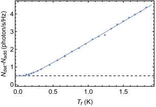
Figure S7: System noise calibration. Measured noise (dots) together with a fit to Eq. (26) (line) shown in units of photons using $N_{\text{det}}-N_{\text{add}}=P_{\text{ESA}}/(\hbar\omega_{e}\beta_{4}\text{BW})-N_{\text{add}}$. The dashed line indicates the half vacuum noise photon added by the measurement.

The microwave transmission line is characterized by the input attenuation $\beta_{3}$, the output gain $\beta_{4}$ and the total added noise of the output line $N_{\text{sys}}$. The output line is first calibrated by using a 50 $\Omega$ load, a resistive heater, and a thermometer that are thermally connected. Weak thermal contact to the mixing chamber of the dilution refrigerator allows to change the temperature $T_{50\Omega}$ of the 50 $\Omega$ load without heating up the mixing chamber. We vary $T_{50\Omega}$ from 21.5 mK to 1.8 K and measure the amplified thermal noise on a spectrum analyzer. The measured power spectral density $P_{\text{ESA}}(\omega)$ is approximately constant around the microwave resonance frequency $\omega_{e}$ and its temperature dependence follows

$$P_{\text{ESA}}=\hbar\omega_{e}\beta_{4}\text{BW}\left(\frac{1}{2}\coth{\left(\frac{\hbar\omega_{e}}{2k_{\text{B}}T_{50\Omega}}\right)}+N_{\text{add}}\right),$$ (26)

where BW stands for the chosen resolution bandwidth, $k_{\text{B}}$ is Boltzmann’s constant and $N_{\text{add}}$ is the effective noise added to the signal at the output port of the device due to amplifiers and losses. At $T_{50\Omega}=0$ K this reduces to $P_{\text{ESA}}=\hbar\omega_{e}\beta_{4}\text{BW}N_{\text{sys}}$ with $N_{\text{sys}}=N_{\text{add}}+0.5$. Figure S7 shows the detected noise $N_{\text{det}}-N_{\text{add}}=P_{\text{ESA}}/(\hbar\omega_{e}\beta_{4}\text{BW})-N_{\text{add}}$ as a function of the load temperature $T_{50\Omega}$. The values for gain and added noise obtained from a fit to Eq. (26) are $67.65\pm 0.05$ dB and $10.66\pm 0.15$ as shown in Fig. S7. The emitted black body radiation undergoes the same losses and gains, as shown in Fig. S1, up an independently calibrated cable length difference right at the sample output resulting in an additional loss of $0.6\pm 0.09$ dB. Taking into account this addition loss we arrive at the corrected gain and system noise $\beta_{4}=67.05\pm 0.16$ dB and $N_{\text{sys}}=12.74\pm 0.36$. For the stated error bars we take into account the 95% confidence interval of the fit, an estimated temperature sensor accuracy of $\pm 2.5\%$ over the relevant range, as well as the estimated inaccuracy in the cable attenuation difference. The input attenuation is then easily deduced from a VNA reflection measurement $|\text{S}_{ee}|^{2}$ that yields $\beta_{3}=-74.92\pm 0.16$ dB.

D.3 Optical calibration

The optical transmission lines consist mainly of two optical single mode fibers. The input optical line starts from the OC2 (see Fig. S1) and terminates at the WGM resonator-prism interface. The output optical line is defined from the WGM resonator-prism interface to the OSA (see Fig. S1). From the measured external conversion efficiencies $\eta_{\text{tot}}$ and the microwave line calibration, we can determine the losses of the input and output transmission lines using

$$\frac{P_{\text{out},o}}{\omega_{o}}=\beta_{2}\eta_{\text{tot}}\beta_{3}\frac{P_{\text{in},e}}{\omega_{e}}$$

$$\frac{P_{\text{out},e}}{\omega_{e}}=\beta_{4}\eta_{\text{tot}}\beta_{1}\frac{P_{\text{in},o}}{\omega_{o}}$$ (27)

where $P_{\text{in},i}$ are the input powers of our transmission lines coming out from OC2 and S2 and $P_{\text{out},i}$ are the measured powers at the end of the transmission lines measured with the OSA and ESA. The procedure yields the input attenuation $\beta_{1}=-4.81$ dB and the output gain (via EDFA) $\beta_{2}=+30.8$ dB. For measurements above $P_{p}=0.1$ mW, we bypass the EDFA by switching OS2, resulting in an output attenuation of $\beta_{2}=-5.5$dB.

D.4 Bidirectionality

Figure S8 shows the measured total conversion efficiency as a function of signal frequency (dots) using Eq. (27) together with theory (lines) using Eq. (6) in both conversion directions for two different pump powers. Because the optical calibration Eq. (27) assumes symmetric bidirectionality we also find that the measurement results are perfectly symmetric. Nevertheless, direct measurements of $\beta_{1}$ taken at room temperature of -2.6 dB are in good agreement with the optical calibration. We attribute the additional loss of up to 2.2 dB to changes in the optical alignment during the cooldown, e.g. in the cold APC connector, as well as reflection loss at the first prism surface that is not included in the room temperature calibration.

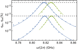
Figure S8: Conversion bandwidth and bidirectionality. Measured total conversion efficiency $\eta_{eo}$ (blue dots) and $\eta_{oe}$ (green dots) as a function of output signal frequency $\omega$ (optics to microwave, blue) or $\omega=\omega_{o}-\omega_{p}$ (microwave to optics, green) for $P_{p}$=18.7 $\mu$W and $P_{p}$=1.48 mW. Microwave-to-optics conversion (green) is displaced by 10 MHz for better visibility. Dashed lines indicate the maxima of the theory curves in agreement with the results reported in the main text.

References

- (1) Hecht, J. City of Light: The Story of Fiber Optics (Oxford University Press, 1999).
- (2) Capmany, J. & Novak, D. Microwave photonics combines two worlds. Nature Photonics 1, 319–330 (2007).
- (3) Matsko, A. B., Savchenkov, A. A., Ilchenko, V. S., Seidel, D. & Maleki, L. On fundamental quantum noises of whispering gallery mode electro-optic modulators. Opt. Express 15, 17401–17409 (2007).
- (4) Tsang, M. Cavity quantum electro-optics. Physical Review A 81, 063837 (2010).
- (5) Tsang, M. Cavity quantum electro-optics. II. Input-output relations between traveling optical and microwave fields. Physical Review A 84, 043845 (2011).
- (6) Rueda, A. et al. Efficient microwave to optical photon conversion: an electro-optical realization. Optica 3, 597–604 (2016).
- (7) Javerzac-Galy, C. et al. On-chip microwave-to-optical quantum coherent converter based on a superconducting resonator coupled to an electro-optic microresonator. Phys. Rev. A 94, 053815 (2016).
- (8) Soltani, M. et al. Efficient quantum microwave-to-optical conversion using electro-optic nanophotonic coupled resonators. Phys. Rev. A 96, 043808– (2017).
- (9) Cohen, D., Hossein-Zadeh, M. & Levi, A. High-q microphotonic electro-optic modulator. Solid-State Electronics 45, 1577–1589 (2001).
- (10) Ilchenko, V. S., Savchenkov, A. A., Matsko, A. B. & Maleki, L. Whispering-gallery-mode electro-optic modulator and photonic microwave receiver. J. Opt. Soc. Am. B 20, 333–342 (2003).
- (11) Fan, L. et al. Superconducting cavity electro-optics: A platform for coherent photon conversion between superconducting and photonic circuits. Science Advances 4 (2018).
- (12) Witmer, J. D. et al. A silicon-organic hybrid platform for quantum microwave-to-optical transduction. Quantum Science and Technology (2020).
- (13) Reed, A. P. et al. Faithful conversion of propagating quantum information to mechanical motion. Nature Physics 13, 1163–1167 (2017).
- (14) Rueda, A., Hease, W., Barzanjeh, S. & Fink, J. M. Electro-optic entanglement source for microwave to telecom quantum state transfer. npj Quantum Information 5, 108– (2019).
- (15) Zhong, C. et al. Proposal for heralded generation and detection of entangled microwave–optical-photon pairs. Phys. Rev. Lett. 124, 010511– (2020).
- (16) Kurpiers, P. et al. Deterministic quantum state transfer and remote entanglement using microwave photons. Nature 558, 264–267 (2018).
- (17) Rueda, A., Sedlmeir, F., Kumari, M., Leuchs, G. & Schwefel, H. G. L. Resonant electro-optic frequency comb. Nature 568, 378–381 (2019).
- (18) Youssefi, A. et al. Cryogenic electro-optic interconnect for superconducting devices (2020). arXiv:eprint 2004.04705.
- (19) Arute, F. et al. Quantum supremacy using a programmable superconducting processor. Nature 574, 505–510 (2019).
- (20) Burkard, G., Gullans, M. J., Mi, X. & Petta, J. R. Superconductor-semiconductor hybrid-circuit quantum electrodynamics. Nature Reviews Physics (2020).
- (21) Awschalom, D. D., Hanson, R., Wrachtrup, J. & Zhou, B. B. Quantum technologies with optically interfaced solid-state spins. Nature Photonics 12, 516–527 (2018).
- (22) Kimble, H. J. The quantum internet. Nature 453, 1023–1030 (2008).
- (23) Wehner, S., Elkouss, D. & Hanson, R. Quantum internet: A vision for the road ahead. Science 362, eaam9288 (2018).
- (24) Lecocq, F., Clark, J. B., Simmonds, R. W., Aumentado, J. & Teufel, J. D. Mechanically mediated microwave frequency conversion in the quantum regime. Phys. Rev. Lett. 116, 043601 (2016).
- (25) Lambert, N. J., Rueda, A., Sedlmeir, F. & Schwefel, H. G. L. Quantum information technologies: Coherent conversion between microwave and optical photons – an overview of physical implementations. Advanced Quantum Technologies 3, 2070011 (2020).
- (26) Lauk, N. et al. Perspectives on quantum transduction. Quantum Science and Technology 5, 020501 (2020).
- (27) Higginbotham, A. P. et al. Harnessing electro-optic correlations in an efficient mechanical converter. Nature Physics 14, 1038–1042 (2018).
- (28) Arnold, G. et al. Converting microwave and telecom photons with a silicon photonic nanomechanical interface. arXiv:2002.11628 (2020).
- (29) Vainsencher, A., Satzinger, K. J., Peairs, G. A. & Cleland, A. N. Bi-directional conversion between microwave and optical frequencies in a piezoelectric optomechanical device. Applied Physics Letters 109, 033107 (2016).
- (30) Jiang, W. et al. Efficient bidirectional piezo-optomechanical transduction between microwave and optical frequency. Nature Communications 11, 1166 (2020).
- (31) Han, X. et al. 10-ghz superconducting cavity piezo-optomechanics for microwave-optical photon conversion (2020). arXiv:eprint 2001.09483.
- (32) Forsch, M. et al. Microwave-to-optics conversion using a mechanical oscillator in its quantum ground state. Nature Physics 16, 69–74 (2020).
- (33) Mirhosseini, M., Sipahigil, A., Kalaee, M. & Painter, O. Quantum transduction of optical photons from a superconducting qubit (2020). arXiv:eprint 2004.04838.
- (34) Strekalov, D. V., Marquardt, C., Matsko, A. B., Schwefel, H. G. L. & Leuchs, G. Nonlinear and quantum optics with whispering gallery resonators. Journal of Optics 18, 123002 (2016).
- (35) Andrews, R. W. et al. Bidirectional and efficient conversion between microwave and optical light. Nature Physics 10, 321–326 (2014).
- (36) Xu, M. et al. Radiative cooling of a superconducting resonator. Phys. Rev. Lett. 124, 033602– (2020).
- (37) Woodcraft, A. L. Recommended values for the thermal conductivity of aluminium of different purities in the cryogenic to room temperature range, and a comparison with copper. Cryogenics 45, 626–636 (2005).
- (38) Fink, J. M. et al. Quantum-to-classical transition in cavity quantum electrodynamics. Phys. Rev. Lett. 105, 163601 (2010).
- (39) Wang, Z. et al. Quantum microwave radiometry with a superconducting qubit. arXiv:1909.12295 (2019).
- (40) Scigliuzzo, M. et al. Primary thermometry of propagating microwaves in the quantum regime. arXiv:2003.13522 (2020).
- (41) Briegel, H.-J., Dür, W., Cirac, J. I. & Zoller, P. Quantum repeaters: The role of imperfect local operations in quantum communication. Phys. Rev. Lett. 81, 5932– (1998).
- (42) Rueda Sanchez, A. R. Resonant Electrooptics. Doctoral thesis, Friedrich-Alexander-Universität Erlangen-Nürnberg (FAU) (2018).
- (43) Wong, K. Properties of Lithium Niobate. EMIS datareviews series (INSPEC, The Institution of Electrical Engineers, London, UK, 2002).