MTFuzz: Fuzzing with a Multi-task Neural Network

Abstract.

Fuzzing is a widely used technique for detecting software bugs and vulnerabilities. Most popular fuzzers generate new inputs using an evolutionary search to maximize code coverage. Essentially, these fuzzers start with a set of seed inputs, mutate them to generate new inputs, and identify the promising inputs using an evolutionary fitness function for further mutation.

Despite their success, evolutionary fuzzers tend to get stuck in long sequences of unproductive mutations. In recent years, machine learning (ML) based mutation strategies have reported promising results. However, the existing ML-based fuzzers are limited by the lack of quality and diversity of the training data. As the input space of the target programs is high dimensional and sparse, it is prohibitively expensive to collect many diverse samples demonstrating successful and unsuccessful mutations to train the model.

In this paper, we address these issues by using a Multi-Task Neural Network that can learn a compact embedding of the input space based on diverse training samples for multiple related tasks (i.e., predicting for different types of coverage). The compact embedding can guide the mutation process by focusing most of the mutations on the parts of the embedding where the gradient is high. MTFuzz uncovers $11$ previously unseen bugs and achieves an average of $2\times$ more edge coverage compared with 5 state-of-the-art fuzzer on 10 real-world programs.

1. Introduction

Coverage-guided graybox fuzzing is a widely used technique for detecting bugs and security vulnerabilities in real-world software (Zalewski, 2017; Darpa, 2016; Zalewski, 2017; Manes et al., 2018; Wang et al., 2019a; Nilizadeh et al., 2019; You et al., 2018; Lemieux and Sen, 2018; She et al., 2019b; Godefroid et al., 2008a; Arya and Neckar, 2012; Evans et al., 2011; Moroz and Serebryany, 2016). The key idea behind a fuzzer is to execute the target program on a large number of automatically generated test inputs and monitor the corresponding executions for buggy behaviors. However, as the input spaces of real-world programs are typically very large, unguided test input generation is not effective at finding bugs. Therefore, most popular graybox fuzzers use evolutionary search to generate new inputs; they mutate a set of seed inputs and retain only the most promising inputs (i.e., inputs exercising new program behavior) for further mutations (Zalewski, 2017; Wang et al., 2019a; Nilizadeh et al., 2019; You et al., 2018; Wei et al., 2018; Li et al., 2017; Godefroid et al., 2017; Lemieux and Sen, 2018; Jiang et al., 2018).

However, the effectiveness of traditional evolutionary fuzzers tends to decrease significantly over fuzzing time. They often get stuck in long sequences of unfruitful mutations, failing to generate inputs that explore new regions of the target program (Chen and Chen, 2018; She et al., 2019b, a). Several researchers have worked on designing different mutation strategies based on various program behaviors (e.g., focusing on rare branches, call context, etc.) (Lemieux and Sen, 2018; Chen and Chen, 2018). However, program behavior changes drastically, not only across different programs but also across different parts of the same program. Thus, finding a generic robust mutation strategy still remains an important open problem.

Recently, Machine Learning (ML) techniques have shown initial promise to guide the mutations (Saavedra et al., 2019; She et al., 2019b; Rajpal et al., 2017). These fuzzers typically use existing test inputs to train ML models and learn to identify promising mutation regions that improve coverage (She et al., 2019b; Godefroid et al., 2017; Rajpal et al., 2017; Saavedra et al., 2019). Like any other supervised learning technique, the success of these models relies heavily on the number and diversity of training samples. However, collecting such training data for fuzzing that can demonstrate successful/unsuccessful mutations is prohibitively expensive due to two main reasons. First, successful mutations that increase coverage are often limited to very few, sparsely distributed input bytes, commonly known as hot-bytes, in a high-dimensional input space. Without knowing the distribution of hot-bytes, it is extremely hard to generate successful mutations over the sparse, high-dimensional input space (She et al., 2019b; Saavedra et al., 2019). Second, the training data must be diverse enough to expose the model to various program behaviors that lead to successful/unsuccessful mutations—this is also challenging as one would require a large number of test cases exploring different program semantics. Thus, the ML-based fuzzers suffer from both sparsity and lack of diversity of the target domain.

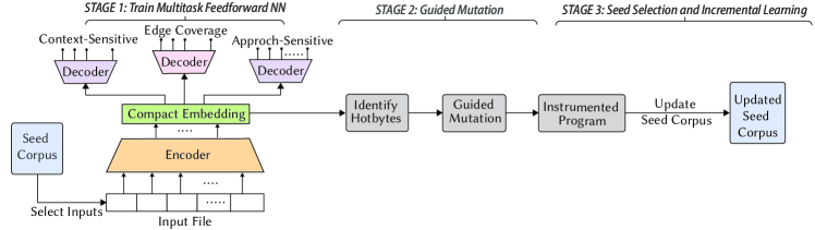
Figure 1. Overview of MTFuzz

In this paper, we address these problems using Multi-Task Learning, a popular learning paradigm used in domains like computer vision to effectively learn common features shared across related tasks from limited training data. In this framework, different participating tasks allow an ML model to effectively learn a compact and more generalized feature representation while ignoring task-specific noises. To jointly learn a compact embedding of the inputs, in our setting, we use different tasks for predicting the relationship between program inputs and different aspects of fuzzing-related program behavior (e.g., different types of edge coverage). Such an architecture addresses both the data sparsity and lack of diversity problem. The model can simultaneously learn from diverse program behaviors from different tasks as well as focus on learning the important features (hot bytes in our case) across all tasks. Each participating task will provide separate pieces of evidence for the relevance or irrelevance of the input features (Ruder, 2017).

To this end, we design, implement, and evaluate MTFuzz, a Multi-task Neural Network (MTNN) based fuzzing framework. Given the same set of test inputs, MTFuzz learns to predict three different code coverage measures showing various aspects of dynamic program behavior:

1. edge coverage: which edges are explored by a test input (Zalewski, 2017; She et al., 2019b)?

2. approach-sensitive edge coverage: if an edge is not explored, how far off it is (i.e., approach level) from getting triggered (McMinn and Holcombe, 2004a; Arcuri, 2010; McMinn, 2011; Pachauri and Srivastava, 2013)?

3. context-sensitive edge coverage: from which call context an explored edge is called (Chen and Chen, 2018; Wang et al., 2019b)?

Note that our primary task, like most popular fuzzers, is to increase edge coverage. However, the use of call context and approach level provides additional information to boost edge coverage.

Architecturally, the underlying MTNN contains a group of hidden layers shared across the participating tasks, while still maintaining task-specific output layers. The last shared layer learns a compact embedding of the input space as shown in Figure 1. Such an embedding captures a generic compressed representation of the inputs while preserving the important features, i.e., hot-byte distribution. We compute a saliency score (She et al., 2019a) of each input byte by computing the gradients of the embedded representation w.r.t. the input bytes. Saliency scores are often used in computer vision models to identify the important features by analyzing the importance of that feature w.r.t. an embedded layer (Simonyan et al., 2013). By contrast, in this paper, we use such saliency scores to guide the mutation process—focus the mutations on bytes with high saliency scores.

Our MTNN architecture also allows the compact embedding layer, once trained, to be transferred across different programs that operate on similar input formats. For example, compact-embedding learned with MTFuzz for one xml parser may be transferred to other xml parsers. Our results (in RQ4) show that such transfer is quite effective and it reduces the cost to generate high quality data from scratch on new programs which can be quite expensive. Our tool is available at https://git.io/JUWkj and the artifacts available at doi.org/10.5281/zenodo.3903818.

We evaluate MTFuzz on 10 real world programs against 5 state-of-the-art fuzzers. MTFuzz covers at least 1000 more edges on 5 programs and several 100 more on the rest. MTFuzz also finds a total of 71 real-world bugs (11 previously unseen) (see RQ1). When compared to learning each task individually, MTFuzz offers significantly more edge coverage (see RQ2). Lastly, our results from transfer learning show that the compact-embedding of MTFuzz can be transferred across parsers for xml and elf binaries.

Overall, our paper makes the following key contributions:

• We present a novel fuzzing framework based on multi-task neural networks called MTFuzz that learns a compact embedding of otherwise sparse and high-dimensional program input spaces. Once trained, we use the salience score of the embedding layer outputs w.r.t. the input bytes to guide the mutation process.

• Our empirical results demonstrate that MTFuzz is significantly more effective than current state-of-the-art fuzzers. On $10$ real world programs, MTFuzz achieves an average of $2\times$ and up to $3\times$ edge coverage compared to Neuzz, the state-of-the-art ML-based fuzzer. MTFuzz also finds $11$ previously unknown bugs other fuzzers fail to find. The bugs have been reported to the developers.

• We demonstrate that transferring of the compact embedding across programs with similar input formats can significantly increase the fuzzing efficiency, e.g., transferred embeddings for different file formats like ELF and XML can help MTFuzz to achieve up to $14\times$ edge coverage compared to state-of-the-art fuzzers.

2. Background: Multi-task Networks

Multi-task Neural Networks (MTNN) are becoming increasingly popular in many different domains including optimization (Argyriou et al., 2008; Gong et al., 2014), natural language processing (Collobert and Weston, 2008; Binge and Sogaard, 2017), and computer vision (Standley et al., 2019). The key intuition behind MTNN is that it is useful for related tasks to be learned jointly so that each task can benefit from the relevant information available in other tasks (Caruana, 1996, 1997; Standley et al., 2019; Zamir et al., 2018). For example, if we learn to ride a unicycle, a bicycle, and a tricycle simultaneously, experiences gathered from one usually help us to learn the other tasks better (Zhang and Yang, 2017). In this paper, we use a popular MTNN architecture called hard parameter sharing (Caruana, 1997), which contain two groups of layers (see Fig. 5): a set of initial layers shared among all the tasks, and several individual task-specific output layers. The shared layers enable a MTNN to find a common feature representation across all the tasks. The task specific layers use the shared feature representation to generate predictions for the individual tasks  (Kokkinos, 2017; Standley et al., 2019; Ruder, 2017).

MTNN Training. While MTNNs can be used in many different ML paradigms, in this paper we primarily focus on supervised learning. We assume that the training process has access to a training dataset $\mathcal{X}=\{x_{1},x_{2},...,x_{n}\}$. The training data contains the ground truth output labels for each task. We train the MTNN on the training data using standard back-propagation to minimize a multi-task loss.

Multi-task Loss. An MTNN is trained using a multi-task loss function, $\mathcal{L}$. We assume that each individual task $\tau_{i}$ in the set of tasks $\mathcal{T}=\{\tau_{1},\tau_{2},...,\tau_{m}\}$ has a corresponding loss function $\mathcal{L}_{i}$. The multi-task loss is computed as a weighted sum of each individual task loss. More formally, it is given by $\mathcal{L}=\sum^{m}_{i=1}\alpha_{i}\cdot\mathcal{L}_{i}$. Here, $\alpha_{i}$ represents the weight assigned to task $i$. The goal of training is to reduce the overall loss. In practice, the actual values of the weights are decided based on the relative importance of each task. Most existing works assign equal weights to the tasks (Uhrig et al., 2016; Teichmann et al., 2018; Liao et al., 2016).

The multi-task loss function forces the shared layer to learn a general input representation for all tasks offering two benefits:

1)  Increased generalizibility. The overall risk of overfitting in multi-task models is reduced by an order of $m$ (where $\mathit{m}$ is the number of tasks) compared to single task models (Baxter, 1997). Intuitively, the more tasks an MTNN learns from, the more general the compact representation is in capturing features of all the tasks. This prevents the representation from overfitting to the task-specific features.

2)  Reduced sparsity. The shared embedding layer in an MTNN can be designed to increase the compactness of the learned input representation. Compared with original input layer, a shared embedding layer can achieve same expressiveness on a given set of tasks while requiring far fewer nodes. In such compact embedding, the important features across different tasks will be boosted with each task contributing its own set of relevant features (Ruder, 2017).

3. Methodology

This section presents a brief overview of MTFuzz that aims to maximize edge coverage with the aid of two additional coverage measures: context-sensitive edge coverage and approach-sensitive edge coverage using multi task learning. Figure 1 illustrates an end-to-end workflow of the proposed approach. The first stage trains an MTNN to produce a compact embedding of an otherwise sparse input space while preserving information about the hot bytes i.e., the input bytes have the highest likelihood to impact code coverage (Section 3.2). The second stage identifies these hot bytes and focuses on mutating them (Section 3.3). Finally, in the third stage, the seed corpus is updated with the mutated inputs and retains only the most interesting new inputs (Section 3.4).

3.1. Modeling Coverage as Multiple Tasks

The goal of any ML-based fuzzers, including MTFuzz, is to learn a mapping between input space and code coverage. The most common coverage explored in the literature is edge coverage, which is an effective measure and quite easy to instrument. However, it is coarse-grained and misses many interesting program behavior (e.g., explored call context) that are known to be important to fuzzing. One workaround is to model path coverage by tracking the program execution path per input. However, keeping track of all the explored paths can be computationally intractable since it can quickly lead to a state-space explosion on large programs (Wang et al., 2019b). As an alternative, in this work, we propose a middle ground: we model the edge coverage as the primary task of the MTNN, while choosing two other fine-granular coverage metrics (approach-sensitive edge coverage and context-sensitive edge coverage) as auxiliary tasks to provide useful additional context to edge coverage.

3.1.1. Edge coverage: Primary Task. 

Edge coverage measures how many unique control-flow edges are triggered by a test input as it interacts with the program. It has become the de-facto code coverage metric (Zalewski, 2017; She et al., 2019b; Lemieux and Sen, 2018; You et al., 2018) for fuzzing. We model edge coverage prediction as the primary task of our multi-task network, which takes a binary test case as input and predicts the edges that could be covered by the test case. For each input, we represent the edge coverage as an edge bitmap, where value per edge is set to 1 or 0 depending on whether the edge is exercised by the input or not.

In particular, in the control-flow-graph of a program, an edge connects two basic blocks (denoted by prev_block and cur_block) (Zalewski, 2017). A unique $edge\_id$ is obtained as: $hash(\texttt{prev\_block},\texttt{cur\_block})$. For each $edge\_id$, there is a bit allocated in the bitmap. For every input, the edge_ids in the corresponding edge bitmap are set to 1 or 0, depending on whether or not those edges were triggered.

3.1.2. Approach-Sensitive Edge Coverage: Auxiliary Task 1. 

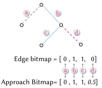
Figure 2. Approach Bitmap vs. Edge Bitmap. The edge ‘d’ has a visited parent edge ‘b’ and is thus marked 0.5 in the approach bitmap.

For an edge that is not exercised by an input, we measure how far off the edge is from getting triggered. Such a measure provides additional contextual information of an edge. For example, if two test inputs failed to trigger an edge, however one input reached “closer” to the unexplored edge than the other, traditional edge coverage would treat both inputs the same. However, using a proximity measure, we can discern between the two inputs and mutate the closer input so that it can reach the unexplored edge. To achieve this, approach-sensitive edge coverage extends edge coverage by offering a distance measure that computes the distance between an unreached edge and the nearest edge triggered by an input. This is a popular measure in the search-based software engineering literature (McMinn and Holcombe, 2004a; McMinn, 2011; Arcuri, 2010), where instead of assigning a binary value (0 or 1), as in edge bitmap, approach level assigns a numeric value between 0 and 1 to represent the edges (McMinn and Holcombe, 2004b); if an edge is triggered, it is assigned 1. However, if the edge is not triggered, but one of its parents are triggered, then the non-triggered edge is assigned a value of $\beta$ (we use $\beta=0.5$). If neither the edge nor any of its parents are triggered, it is assigned $0$. This is illustrated in Fig. 2. Note that, for a given edge, we refrain from using additional ancestors farther up the control-flow graph to limit the computational burden. The approach sensitive coverage is represented in an approach bitmap, where for every unique $edge\_id$, we set an approach level value, as shown in Fig. 2. We model this metric in our Multi-task Neural Network as an auxiliary task, where the task takes binary test cases as inputs and learn to predict the corresponding approach-level bitmaps.

3.1.3. Context-sensitive Edge Coverage: Auxiliary Task 2. 

Edge coverage cannot distinguish between two different test inputs triggering the same edge, but via completely different internal states (e.g., through the same function called from different sites in the program). This distinction is valuable since reaching an edge via a new internal state (e.g., through a new function call site) may trigger a vulnerability hidden deep within the program logic. Augmenting edge coverage with context information regarding internal states of the program may help alleviate this problem (Chen and Chen, 2018).

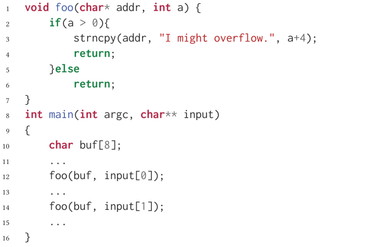
Figure 3. An example C-code to demonstrate the usefulness of using context-sensitive measures. Measures such as edge coverage will fail to detect a possible bug in strncpy($\cdot$)

Consider the example in Fig. 3. Here, for an input [1, 0], the first call to function foo() appears at site line 12 and it triggers the if condition (on line 2); the second call to foo() appears on site line 14 and it triggers the else condition (on line 5). As far as edge coverage is concerned, both the edges of the function foo() (on lines 2 and 5) have been explored and any additional inputs will remain uninteresting. However, if we provide a new input say [0, 8], we would first trigger line 5 of foo when it is called from line 12. Then we trigger line 2 of foo from line 14 and further cause a buffer overflow at line 3 because a 12 bytes string is written into a 8 bytes destination buffer buf. Moveover, the input [0, 8] will not be saved by edge coverage fuzzer since it triggers no new edges. Frequently called functions (like strcmp) may be quite susceptible such crashes (Wang et al., 2019b).

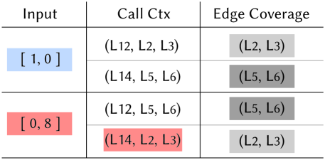
Figure 4. The tuple in edge coverage does not differentiate between the clean input and the buggy input, while of context-sensitive edge coverage (labeled ‘Call Ctx’) does.

In order to overcome this challenge, Chen et al. (Chen and Chen, 2018) propose keeping track of the call stack in addition to the edge coverage by maintaining tuple: $(\textit{call\_stack},\textit{prev\_block},\textit{cur\_block})$. Fig. 4 shows the additional information provided by context-sensitive edge coverage over edge coverage. Here, we see an example where a buggy input [0,8] has the exact same edge coverage as the clean input [1,0]. However, the call context information can differentiate these two inputs based on the call stacks at line 12 and 14.

We model context-sensitive edge coverage in our framework as an auxiliary task. We first assign a unique id to every call. Next, at run time, when we encounter a call at an edge ($edge\_id$), we first compute a $hash$ to record all the functions on current call stack as: $call\_stack=call\_id_{1}\oplus...\oplus call\_id_{n}$, where $call\_id\_i$ represents the $\mathit{i}$-th function on current call stack and $\oplus$ denotes XOR operation. Next, we compute the context sensitive edge id as: $call\_trace\_id=call\_stack\oplus edge\_id$.

Thus we obtain a unique $call\_trace\_id$ for every function called from different contexts (i.e., call sites). We then create a bit-map of all the $call\_trace\_id$s. Unlike existing implementations of context-sensitive edge coverage (Chen and Chen, 2018; Wang et al., 2019b), we assign an additional id to each call instruction while maintaining the original $edge\_id$ intact. Thus, the total number of elements in our bit map reduces to sum of $call\_trace\_id$s and $edge\_id$s rather than a product of $call\_trace\_id$s and $edge\_id$s. An advantage of our design is that we minimize the bitmap size. In practice, existing methods requires around $7\times$ larger bitmap size than just edge coverage (Chen and Chen, 2018); our implementation only requires around $1.3\times$ bitmap size of edge coverage. The smaller bitmap size can avoid edge explosion and improve performance.

In our multi-tasking framework, the context-sensitive edge coverage “task” is trained to predict the mapping between the inputs and the corresponding $call\_trace\_id$s bitmaps. This can enable us to learn the difference between two inputs in a more granular fashion. For example, an ML model can learn that under certain circumstances, the second input byte (input[1] in Fig. 3) can cause crashes. This information cannot be learned by training to predict for edge coverage alone since both inputs will have the same edge coverage (as shown in Fig. 4).

3.2. Stage-I: Multi-Task Training

This phase builds a multi-task neural network (MTNN) that can predict different types of edge coverage given a test input. The trained model is designed to produce a more general and compact embedding of the input space focusing only on those input bytes that are most relevant to all the tasks. This compact representation will be reused by the subsequent stages of the program to identify the most important bytes in the input (i.e., the hot-bytes) and guide mutations on those bytes.

3.2.1. Architecture. 

Fig. 5 shows the architecture of the MTNN. The model contains an encoder (shared among all the tasks) and three task-specific decoders. The model takes existing test input bytes as input and outputs task-specific bitmap. Each input byte corresponds to one input node, and each bitmap value corresponds to an ouput node.

Encoder. Comprises of one input layer followed by three progressively narrower intermediate layers. The total number of nodes in the input layer is equal to the total number of bytes in the largest input in the seed corpus. All shorter inputs are padded with 0x00 for consistency. The last layer of the encoder is a compact representation of the input to be used by all the tasks (green in Fig. 5). Decoders. There are three task-specific decoders (shown in lilac in Fig. 5). Each task specific decoder consists of three intermediate layers that grow progressively wider. The last layer of each of the decoder is the output layer. For edge coverage, there is one node in the output layer for each unique $edge\_id$, likewise for context-sensitive edge coverage there is one output node for each $call\_trace\_id$, and for approach-sensitive edge coverage there is one output node for each unique $edge\_id$ but they take continuous values (see Fig. 2).

3.2.2. Loss functions. 

The loss function of a MTNN is a weighted sum of the task-specific loss functions. Among our three tasks, edge coverage and context-sensitive edge coverage are modeled as classification tasks and approach-sensitive edge coverage is modeled as a regression task. Their loss functions are designed accordingly.

Loss function for approach-sensitive edge coverage. Approach-level measures how close an input was from an edge that was not triggered. This distance is measured using a continuous value between 0 and 1. Therefore, this is a regression problem and we use mean squared error loss, given by:

(1) $$\mathcal{L}_{\tau_{\text{\tiny approach}}}=\operatorname{MSE}=\frac{1}{n}\sum_{i=1...n}(Y_{i}-\hat{Y_{i}})^{2}.$$

Where $Y_{i}$ is the prediction and $\hat{Y_{i}}$ is the ground truth.

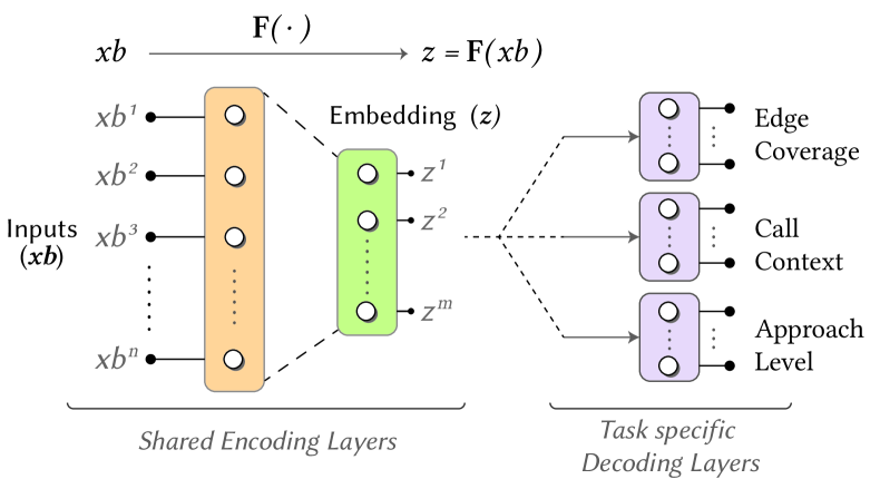
Figure 5. The MTNN architecture representing the n-dimensional input layer $\mathbf{xb^{i}\in xb}$; m-dimensional compact embedding layer $\mathbf{z^{j}\in z}$, s.t. $\mathbf{m<n}$, with a function $\mathbf{F(\cdot)}$ to map input $\mathbf{xb}$ and the embedding layer $\mathbf{xb}$; three task-specific layers.

Loss functions for edge coverage and context-sensitive edge coverage. The outputs of both these tasks are binary values where 1 means an input triggered the $edge\_id$ or the $call\_trace\_id$ and 0 otherwise. We find that while some $edge\_id$s or $call\_trace\_id$s are invoked very rarely, resulting in imbalanced classes. This usually happens when an input triggers a previously unseen (rare) edges. Due to this imbalance, training with an off-the-shelf loss functions such as cross entropy is ill suited as it causes a lot of false negative errors often missing these rare edges.

To address this issue, we introduce a parameter called penalty (denoted by $\beta$) to penalize these false negatives. The penalty is the ratio of the number of times an edge is not invoked over the number of times it is invoked. That is,

$$\small\text{Penalty}=\beta_{\tau}=\frac{\text{\# times an edge\_id (or call\_trace\_id) is {not} invoked}}{\text{\# times an edge\_id (or call\_trace\_id) is invoked}}$$

Here, $\beta_{\tau}$ represents the penalty for every applicable task $\tau$$\in$$\mathcal{T}$ and it is dynamically evaluated as fuzzing progresses. Using $\beta_{\tau}$ we define an adaptive loss for classification tasks in our MTNN as:

(2) $$\mathcal{L}_{\tau_{\text{\tiny ec/ctx}}}=-\sum_{\text{edge}}\left(\beta_{\tau}\cdot p\cdot log(\hat{p})+(1-p)\cdot log(1-\hat{p})\right)\vspace{-2mm}$$

In Eq. 2, $\mathcal{L}_{\tau_{\text{\tiny ec/ctx}}}$ results in two separate loss functions for edge coverage and context-sensitive edge coverage. The penalty ($\beta_{\tau}$) is used to penalize false-positive and false-negative errors. $\beta_{\tau}>1$ penalizes $p\cdot log({\hat{p}})$, representing false negatives; $\beta_{\tau}=1$ penalizes both false positives and false negatives equally; and $\beta_{\tau}<1$ penalizes $(1-p)\cdot log({1-\hat{p}})$, representing false positives. With this, we compute the total loss for our multi-task NN model with $K$ tasks:

(3) $$\mathcal{L}_{total}=-\sum_{i=1}^{K}\alpha_{i}\mathcal{L}_{i}$$

This is the weighted sum of the adaptive loss $\mathcal{L}_{i}$ for each individual task. Here, $\alpha_{i}$ presents the weight assigned to task $i$.

3.3. Stage-II: Guided Mutation

This phase uses the trained MTNN to generate new inputs that can maximize the code coverage. This is achieved by focusing mutation on the byte locations in the input that can influence the branching behavior of the program (hot-bytes).

We use the the compact embedding layer of the MTNN (shown in green in Fig. 5) to infer the hot-byte distribution. The compact embedding layer is well suited for this because it (a) captures the most semantically meaningful features (i.e., bytes) in the input in a compact manner; and (b) learns to ignore task specific noise patterns (Kumar et al., 2017) and pays more attention to the important bytes that apply to all tasks (Chen et al., 2016; Kulkarni et al., 2015; Bengio et al., 2013).

Formally, we represent the input (shown in orange in Fig. 5) as a byte vector $\mathbf{xb}=\{xb^{1},xb^{2},...,xb^{n}\}\in\mathrm{\left[0,255\right]^{n}}$, where $xb^{i}$ is the $i^{\text{th}}$ byte in $\mathbf{xb}$ and $n$ represents the input dimensions (i.e., number of bytes). Then, after the MTNN has been trained, we obtain the compact embedding layer $\mathbf{z}=\{z^{1},z^{2},...,z^{m}\}$ consisting of $\mathit{m}$ nodes.

Note that when input bytes in $\mathbf{xb}$ changes, $\mathbf{z}$ changes accordingly. The amount of the change is determined by how influential each byte in the input is to all the tasks in the MTNN model. Changes to the hot-bytes, which are more influential, will result in larger changes to $\mathbf{z}$. We use this property to discover the hot-bytes.

To determine how influential each byte in $\mathbf{xb}$ is, we compute the partial derivatives of the nodes in compact layer with respect to all the input bytes. The partial derivative of the $j$-th node in the embedding layer with respect to the $\mathit{i}$-th input byte is:

(4) $$\nabla_{\mathbf{xb}}\leavevmode\nobreak\ \mathbf{z}=\left[\dfrac{\partial f_{j}(\mathbf{x})}{xb^{i}}\right]=\left[\dfrac{\partial z^{j}}{\partial xb^{i}}\right]_{i=1\ldots n,\leavevmode\nobreak\ j=1\dots m}$$

In order to infer the importance of each byte $xb^{i}\in xb$, we define a saliency score for each byte, denoted by $\mathbf{\mathrm{S}}(xb^{i})$. We compute the saliency score as follows:

(5) $$\mathbf{\mathrm{S}}(xb^{i})={{\sum}}_{j=1}^{m}\left|\dfrac{\partial z^{j}}{\partial xb^{i}}\right|\hskip 12.00003pti=1\dots n$$

The saliency score $\mathbf{\mathrm{S}}(xb^{i})$ is the sum of all the partial derivatives in $\nabla_{\mathbf{xb}}\leavevmode\nobreak\ \mathbf{z}$ w.r.t. to the byte $xb^{i}$. The numeric value of each of the $\mathit{n}$ elements in $\mathrm{S}(\mathbf{xb})$ determines the hotness of each byte. The larger the saliency score of an input byte $xb^{i}$ is, the more likely it is to be a hot-byte. Using the saliency score, we can now mutate a test input to generate new ones. To do this, we identify the $\mathit{top-k}$ bytes with the largest saliency values—these are the byte-locations that will be mutated by our algorithm.

For each selected byte-locations, we create a new mutated input by changing the bytes to all permissible values between 0 and 255. Since this only happens to the $\mathit{top-k}$ hot-bytes, the number of newly mutated seeds remains manageable. We use these mutated inputs for fuzzing and monitor various coverage measures.

3.4. Stage-III: Seed Selection & Incremental Learning

In this step, MTFuzz samples some of the mutated inputs from the previous stage to retrain the model. Sampling inputs is crucial as the choice of inputs can significantly affect the fuzzing performance. Also, as fuzzing progresses, the pool of available inputs keeps growing in size. Without some form of sampling strategy, training the NN and computing gradients would take prohibitively long.

To this end, we propose an importance sampling (Owen, 2013) strategy where inputs are sampled such that they reach some important region of the control-flow graph instead of randomly sampling from available input. In particular, our sampling strategy first retains all inputs that invoke previously unseen edges. Then, we sort all the seen edges by their rarity. The rarity of an edge is computed by counting how many inputs trigger that specified edge. Finally, we select the top $T$-rarest edges and include at least one input triggering each of these rare edges. We reason that, by selecting the inputs that invoke the rare edges, we may explore deeper regions of the program on subsequent mutations. In order to limit the number of inputs sampled, we introduce a sampling budget $K$ that determines how many inputs will be selected per iteration.

Using these sampled inputs, we retrained the model periodically to refine its behavior—as more data is becoming available about new execution behavior, retraining makes sure the model has knowledge about them and make more informed predictions.

4. Evaluation

Table 1. Test programs used in our study

Programs		# Lines	MTFuzz train (s)	Initial coverage
Class	Name
binutils-2.30 ELF Parser	readelf -a	21,647	703	3,132
	nm -C	53,457	202	3,031
	objdump -D	72,955	703	3,939
	size	52,991	203	1,868
	strip	56,330	402	3,991
TTF	harfbuzz-1.7.6	9,853	803	5,786
JPEG	libjpeg-9c	8,857	1403	1,609
PDF	mupdf-1.12.0	123,562	403	4,641
XML	libxml2-2.9.7	73,920	903	6,372
ZIP	zlib-1.2.11	1,893	107	1,438

Table 2. State-of-the art fuzzers used in our.

Fuzzer	Technical Description
AFL (Zalewski, 2017)	evolutionary search
AFLFast (Böhme et al., 2017)	evolutionary + markov-model-based search
FairFuzz (Lemieux and Sen, 2018)	evolutionary + byte masking
Angora (Chen and Chen, 2018)	evolutionary + dynamic-taint-guided + coordinate descent + type inference
Neuzz (She et al., 2019b)	Neural smoothing guided fuzzing

Implementation.   Our MTNN model is implemented in Keras-2.2.3 with Tensorflow-1.8.0 as a backend (Abadi et al., 2016; Chollet et al., 2015). The MTNN is based on a feed-forward model, composed of one shared encoder and three independent decoders. The encoder compresses an input file into a $512$ compact feature vector and feeds it into three following decoders to perform different task predictions. For encoder, we use three hidden layers with dimensions 2048, 1024 and 512. For each decoder, we use one final output layer to perform corresponding task prediction. The dimension of final output layer is determined by different programs. We use ReLU as activation function for all hidden layers. We use sigmoid as the activation function for the output layer. For task specific weights, set each task to equal weight ($\alpha_{\tau}=1$ in Eq. 3). The MTNN model is trained for 100 epochs achieving a test accuracy of around $95\%$ on average. We use Adam optimizer with a learning rate of 0.001. As for other hyperparameters, we choose k=1024 for $top-K$ hot-bytes. For seed selection budget $T$ in Stage-III (§3.4), we use $T=750$ input samples where each input reaches atleast one rare edge. We note that all these parameters can be tuned in our replication package.

To obtain the various coverage measures, we implement a custom LLVM pass. Specifically, we instrument the first instruction of each basic block of tested programs to track edge transition between them. We also instrument each call instructions to record the calling context of tested programs at runtime. Additionally, we instrument each branch instructions to measure the distance from branching points to their corresponding descendants. As for magic constraints, we intercept operands of each CMP instruction and use direct-copy to satisfy these constraints.

Study Subjects.  We evaluate MTFuzz on 10 real-world programs, as shown in Table 2. To demonstrate the performance of MTFuzz, we compare the edge coverage and number of bugs detected by MTFuzz with $5$ state-of-the-art fuzzers listed in Table 2. Each state-of-the-art fuzzer was run for 24 hours. The training, retraining, and fuzzing times are included in the total 24 runs for each fuzzer. Training time for MTFuzz is shown in Table 2. MTFuzz and Neuzz both use the same initial seeds for the the approaches and the same fuzzing backend for consistency. We ensure that all other experimental settings were also identical across all studied fuzzers.

Experimental Setup.  All our measurements are performed on a system running Ubuntu 18.04 with Intel Xeon E5-2623 CPU and an Nvidia GTX 1080 Ti GPU. For each program tested, we run AFL-2.52b (Zalewski, 2017) on a single core machine for an hour to collect training data. The average number of training inputs collected for $10$ programs is around $2K$. We use 10KB as the threshold file size for selecting our training data from the AFL input corpus (on average 90% of the files generated by AFL were under the threshold).

5. Experimental Results

We evaluate MTFuzz with the following research questions:

• RQ1: Performance. How does MTFuzz perform in comparison with other state-of-the-art fuzzers?

• RQ2: Contributions of Auxiliary Tasks. How much does each auxiliary task contribute to the overall performance of MTFuzz?

• RQ3: Impact of Design Choices. How do various design choices affect the performance of MTFuzz?

• RQ4: Transferrability. How transferable is MTFuzz?

RQ1: Performance

We compare MTFuzz wiht other fuzzers (from Table 2) in terms of the number of real-world and synthetic bugs detected (RQ1-A and RQ1-B), and edge coverage (RQ1-C).

RQ1-A. How many real world bugs are discovered by MTFuzz compared to other fuzzers?

Evaluation. To evaluate the number of bugs discovered by a fuzzer, we first instrument the program binaries with AddressSanitizer (asa, 2020) and UnderfinedBehaviorSanitizer (ubs, 2020). Such instrumentation is necessary to detect bugs beyond crashes. Next, we run each of the fuzzers for 24 hours (all fuzzers use the same seed corpus) and gather the test inputs generated by each of the fuzzers. We run each of these test inputs on the instrumented binaries and count the number of bugs found in each setting. Finally, we use the stack trace of bug reports generated by two sanitizers to categorize the found bugs. Note, if multiple test inputs trigger the same bug, we only consider it once. Table 3 reports the results.

Observations.  We find that:

1. MTFuzz finds a total of 71 bugs, the most among other five fuzzers in 7 real world programs. In the remaining three programs, no bugs were detected by any fuzzer after 24 hours.

2. Among these, 11 bugs were previously unreported.

Among the other fuzzers, Neuzz (another ML-based fuzzer) is the second best fuzzer, finding 60 bugs. Angora finds 58. We observe that the 11 new bugs predominantly belonged to 4 types: memory leak, heap overflow, integer overflow, and out-of-memory. Interestingly, MTFuzz discovered a potentially serious heap overflow vulnerability in mupdf that was not found by any other fuzzer so far (see Figure 6). A mupdf function ensure_solid_xref allocates memory (line 10) for each object of a pdf file and fills content to these memory chunks (line 14). Prior to that, at line 6, it tries to obtain the total number of objects by reading a field value xref->num_objects which is controlled by program input: a pdf file. MTFuzz leverages gradient to identify the hot bytes which control xref->num_objects and sets it to a negative value. As a result, num maintains its initial value $1$ as line 6 if check fails. Thus, at line 10, the function allocates memory space for a single object as $num=1$. However, in line 14, it tries to fill more than one object to new_sub->table and causes a heap overflow. This bug results in a crash and potential DoS if mupdf is used in a web server.

Table 3. Real-world bugs found after 24 hours by various fuzzers. MTFuzz finds the most number of bugs, i.e., 71 (11 unseen) comprised of 4 heap-overflows, 3 Memory leaks, 2 integer overflows, and 2 out-of-memory bugs.

2 Program	AFLFast	AFL	FairFuzz	Angora	Neuzz	MTFuzz
2 readelf	5	4	5	16	16	17
nm	7	8	8	10	9	12
objdump	6	6	8	5	8	9
size	4	4	5	7	6	10
strip	5	7	9	20	20	21
libjpeg	0	0	0	0	1	1
mupdf	0	0	0	0	0	1
2 Total	27	29	35	58	60	71
2

Table 4. Synthetic bugs in LAVA-M dataset found after 5 hours.

2 Program	#Bugs	Angora	Neuzz	MTFuzz
2 base64	44	48	48	48
md5sum	57	57	60	60
uniq	28	29	29	29
who	2136	1541	1582	1833
2

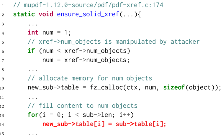
Figure 6. Heap overflow bug in mupdf. The red line shows the bug.

RQ1-B. How many synthetic bugs in LAVA-M dataset are discovered by MTFuzz compared to other fuzzers?

Evaluation. LAVA-M is a synthetic bug benchmark where bugs are injected into four GNU coreutil programs (lava). Each bug in LAVA-M dataset is guarded by a magic number condition. When the magic verification is passed, the corresponding bug will be triggered. Following conventional practice, we run  MTFuzz and other fuzzers from Table 2 on LAVA-M dataset for a total of 5 hours. We measure the number of bugs triggered by each of the state-of-the-art fuzzers. The result is tabulated in  Table 4.

Observations. MTFuzz discovered the most number of bugs on all 4 programs after 5 hours run. The better performance is attributed to the direct-copy module. To find a bug in LAVA-M dataset, fuzzers need to generate an input which satisfies the magic number condition. MTFuzz’s direct-copy module is very effective to solve these magic number verification since it can intercept operands of each CMP instruction at runtime and insert the magic number back into generated inputs.

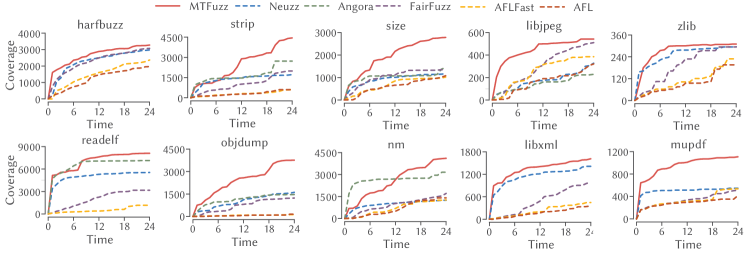
Figure 7. Edge coverage over 24 hours of fuzzing by MTFuzz and other state-of-the-art fuzzers.

Table 5. The average edge coverage of MTFuzz compared with other fuzzers after 24 hours runs for 5 repetitions. Parenthesized numbers represent the standard deviation.

(a) Program binaries compiled with afl-clang-fast

2 Program	MTFuzz	Neuzz	Angora	FairFuzz	AFL	AFLFast
1.5 readelf	8,109	5,953	7,757	3,407	701	1,232
	(286)	(141)	(248)	(1005)	(87)	(437)
nm	4,112	1,245	3,145	1,694	1,416	1,277
	(161)	(32)	(2033)	(518)	(144)	(18)
objdump	3,762	1,642	1,465	1,225	163	134
	(359)	(77)	(148)	(316)	(25)	(15)
size	2,786	1,170	1,586	1,350	1,082	1,023
	(69)	(45)	(204)	(47)	(86)	(117)
strip	4,406	1,653	2,682	1,920	596	609
	(234)	(110)	(682)	(591)	(201)	(183)
libjpeg	543	328	201	504	327	393
	(19)	(34)	(42)	(101)	(99)	(21)
libxml	1,615	1,419	$\cdot$	956	358	442
	(28)	(76)	$\cdot$	(313)	(71)	(41)
mupdf	1,107	533	$\cdot$	503	419	536
	(26)	(76)	$\cdot$	(76)	(28)	(30)
zlib	298	297	$\cdot$	294	196	229
	(38)	(44)	$\cdot$	(95)	(41)	(53)
harfbuzz	3,276	3,000	$\cdot$	3,060	1,992	2,365
	(140)	(503)	$\cdot$	(233)	(121)	(147)
2

$\mathbf{\cdot}$ indicates cases where Angora failed to run due to the external library issue.

(b) Program binaries compiled with alf-gcc

2 Programs	MTFuzz	Neuzz	Angora	FairFuzz	AFL	AFLFast
1.5 readelf	6,701	4,769	6,514	3,423	1,072	1,314
nm	4,457	1,456	2,892	1,603	1,496	1,270
objdump	5,024	2,017	1,783	1,526	247	187
size	3,728	1,737	2,107	1,954	1,426	1,446
strip	6,013	2,726	3,112	3,055	764	757
libjpeg	1,189	719	499	977	671	850
libxml	1,576	1,357	$\cdot$	1,021	395	388
mupdf	1,107	533	$\cdot$	503	419	536
zlib	298	297	$\cdot$	294	196	229
harfbuzz	6,325	5,629	$\cdot$	5,613	2,616	3,692
2

RQ1-C. How much edge coverage does MTFuzz achieve compared to other fuzzers?

Evaluation.  To measure edge coverage, we run each of the fuzzers for 24 hours (all fuzzers use the same seed corpus). We periodically collect the edge coverage information of all the test inputs for each fuzzer using AFL’s coverage report toolkit afl-showmap (Zalewski, 2017). AFL provides coverage instrumentation scheme in two mainstream compilers GCC and Clang. While some authors prefer to use afl-gcc (She et al., 2019b; Lemieux and Sen, 2018; Böhme et al., 2017), some others use afl-clang-fast(Chen and Chen, 2018; Gan et al., 2020). The underlying compilers can have different program optimizations which affects how edge coverage is measured. Therefore, in order to offer a fair comparison with previous studies, we measure edge coverage on binaries compiled with with both afl-gcc and afl-clang-fast. In the rest of the paper, we report results on programs compiled with afl-clang-fast. We observed similar findings with afl-gcc.

Observations.  The results for edge coverage after 24 hours of fuzzing are tabulated in Table 5. The edge-coverage gained over time is shown in Fig. 7. Overall, MTFuzz achieves noticeably more edge coverage than all other baseline fuzzers. Consider the performance gains obtained over the following families of fuzzers:

$\circ$ Evolutionary fuzzers: MTFuzz outperforms all the three evolutionary fuzzers studied here. MTFuzz outperforms Angora on the 6 programs which Angora supports and achieves up to $2297$ more edges in objdump. Note, Angora can’t run on some programs due to the external library issue on its taint analysis engine (Chen and Chen, 2018; Aschermann et al., 2019). When compared to both FairFuzz and AFLFast, MTFuzz covers significantly more edges, e.g., $4702$ more than FairFuzz in readelf and over 28.1$\times$ edges compared to AFLFast on objdump.

$\circ$ Machine learning based fuzzers: In comparison with the state-of-the-art ML based fuzzer, Neuzz (She et al., 2019b), we observed that MTFuzz achieves much greater edge coverage in all 10 programs studied here. We notice improvements of 2000 more edges in readelf and 2500 more edges in nm and strip.

MTFuzz found 71 real-world bugs (11 were previously unknown) and also reach on average $1,277$ and up to $2,867$ more edges compared to Neuzz, the second-best fuzzer, on $10$ programs.

RQ2: Contributions of Auxiliary Tasks

MTFuzz is comprised of an underlying multi-task neural network (MTNN) that contains one primary task (edge coverage) and two auxiliary tasks namely, context-sensitive edge coverage and approach-sensitive edge coverage. A natural question that arises is—How much does each auxiliary task contributes to the overall performance?

Evaluation. To answer this question, We study what would happen to the edge coverage when one of the auxiliary tasks is excluded from the MTFuzz. For this, we build four variants of MTFuzz:

1. (EC): A single-task NN with only the primary task to predict edge coverage.

2. (EC, Call Ctx): An MTNN with edge coverage as the primary task and context-sensitive edge coverage as the auxiliary task.

3. (EC, Approach): An MTNN with edge coverage as the primary task and approach-sensitive edge coverage as the auxiliary task.

4. MTFuzz: Our proposed model with edge coverage as the primary task and two auxiliary tasks context-sensitive edge coverage and approach-sensitive edge coverage.

To rule out other confounders, we ensure that each setting shares the same hyper-parameters and the same initial seed corpus. Also, we ensure that all subsequent steps in fuzzing remain the same across each experiment. With these settings, we run each of the above multi-task models on all our programs from Table 2 for 1 hour to record the edge coverage for each of these MTNN models. Observations. Our results are tabulated in Table 6. We make the following noteworthy observations:

Table 6. Edge coverage after 1 hour. The most improvement to edge coverage is observed when including both the auxiliary tasks are trained together as a multi-task learner.

2 Programs	EC	EC, Call Stack	EC, Approach	MTFuzz
1.5 readelf	4,012	4,172	4,044	4,799
nm	546	532	412	577
objdump	605	632	624	672
size	350	404	500	502
strip	744	787	902	954
harfbuzz	593	661	752	884
libjpeg	190	135	182	223
mupdf	252	193	257	269
libxml2	525	649	677	699
zlib	56	33	59	67
2

1. Fuzzer that uses an MTNN trained on edge coverage as the primary task and context-sensitive edge coverage as the only auxiliary task tends to perform only marginally better than a single task NN based on edge coverage. In some cases, e.g., in Table 6 we notice about 25% more edges. However, in some other cases, for example libjpeg, we noticed that the coverage reduces by almost $31\%$.

2. The above trend is also observable for using edge coverage with approach-sensitive edge coverage as the auxiliary. For example, in libjpeg, the edge coverage is lower than the single-task model that uses only edge coverage.

3. However, MTFuzz, which uses both context-sensitive edge coverage and approach-sensitive edge coverage as auxiliary tasks to edge coverage, performs noticeably better than all other models with up to 800 more edges covered ($\mathbf{\approx}$20%) in the case of readelf.

The aforementioned behavior is expected because each auxiliary task provides very specific albeit somewhat partial context to edge coverage. Context-sensitive edge coverage only provides context to triggered edges, while approach-sensitive edge coverage only reasons about non-triggered edges (see §3.1 for details). Used in isolation, a partial context does not have much to offer. However, while working together as auxiliary tasks along with the primary task, it provides a better context to edge coverage resulting in overall increased edge coverage (see the last column of Table 6).

MTFuzz benefits from both the auxiliary tasks. Using context-sensitive edge coverage and edge coverage along with the primary task (of predicting edge coverage) is most beneficial. We achieve up to 20% more edge coverage.

RQ3. Impact of Design Choices

While building MTFuzz, we made few key design choices such as using a task-specific adaptive loss (§3.2.2) to improve the quality of the multi-task neural network (MTNN) model and a novel seed selection strategy based on importance sampling (see §3.4). Here we assess how helpful these design choices are.

RQ3-A. What are the benefits of using adaptive loss?

MTNN model predicting for edge coverage and for context-sensitive edge coverage tends to experience severely imbalanced class labels. Consider the instance when a certain input triggers an edge for the first time. This is an input of much interest because it represents a new behaviour. The MTNN model must learn what lead to this behaviour. However, in the training sample, there exists only one positive sample for this new edge in the entire corpus. An MTNN that is trained with an off-the-shelf loss functions is likely to misclassify these edges resulting in a false negative error. Such false negatives are particularly damaging because a large number of new edge discoveries go undetected affecting the overall model performance. To counter this, we defined an adaptive loss in §3.2.2; here we measure how much it improves the MTNN’s performance.

Evaluation.  To evaluate the effect of class imbalance, we measure recall which is high when the overall false negatives (FN) are low. While attempting to minimize FNs the model must not make too many false positive (FP) errors. Although false positives are not as damaging as false negatives, we must attempt to keep them low. We therefore also keep track of the F1-scores which quantify the trade-off between false positives and false negatives. We train MTFuzz with two different losses (i.e., with our adaptive loss and with the default cross-entropy loss) on $10$ programs for $100$ epochs and record the final recall and F-1 scores.

Observations. The result are shown in Table 7. We observe that adaptive loss results in MTNNs with an average of $\mathbf{90\%}$ recall score on $10$ programs, while the default loss model only achieves on average $75\%$ recall score. Generally, we notice improvements greater than $\mathbf{15\%}$ over default loss functions. The low recall for default loss function indicates that it is susceptible to making a lot of false negative predictions. However, our adaptive loss function is much better at reducing false negative predictions. Also, the adaptive loss model achieves on average F-1 score of $72\%$, while unweighted loss model achieves an average of $70\%$. This is encouraging because even after significantly reducing the number of false negatives, we maintain the overall performance of the MTNN.

Weighted loss improves MTFuzz’s recall by more than 15%.

RQ3-B. How does seed-selection help?

Evaluation. Here, we evaluate our seed selection strategy (§3.4) by comparing it to a random selection strategy. Specifically, we run two variants of MTFuzz, one with importance sampling for seed selection and the other with a random seed selection. All other components of the tool such as MTNN model, hyperparameters, random seed, etc. are kept constant. We measure the edge coverage obtained by both the strategies on 10 programs after fuzzing for one hour. Table 7 shows the results.

Observations. When compared to a random seed selection strategy. Importance sampling outperforms random seed selection in all $10$ programs offering average improvements of $1.66\times$ more edges covered than random seed selection—for readelf, it covers around $2000$ more edges. This makes intuitive sense because, the goal of importance sampling was to retain the newly generated inputs that invoke certain rare edges. By populating the corpus with such rare and novel inputs, the number of newly explored edges would increase over time, resulting in increase edge coverage (see Table 7).

Table 7. Impact of design choices. Adaptive loss (§3.2.2) increases Recall by $\mathbf{\sim 15\%}$ while maintaining similar F1-scores. Seed selection based in importance sampling (§3.4) demonstrate notable gains in overall edge coverage.

2	Adaptive		Default		Seed Selection
Programs	Recall(%)	F1(%)	Recall(%)	F1(%)	Our Approach	Random
2 readelf	88	68	74	66	4,799	2,893
nm	89	62	69	62	577	269
objdump	89	72	65	71	672	437
size	94	81	78	78	502	312
strip	89	73	80	72	954	545
harfbuzz	92	67	80	71	884	558
libjpeg	88	68	65	65	223	124
mupdf	92	84	90	84	269	160
libxml2	90	70	76	69	699	431
zlib	86	70	70	65	67	57
2

Importance sampling helps MTFuzz achieve on average $1.66\times$ edge coverage compared with random seed selection.

RQ4. Transferability

In this section, we explore the extent to which MTFuzz can be generalized across different programs operating on the same inputs (e.g., two ELF fuzzers). Among such programs, we study if we can transfer inputs generated by fuzzing from one program to trigger edge coverage in another program (RQ4-A) and if it is possible to transfer the shared embedding layers between programs (RQ4-B).

RQ4-A. Can inputs generated for one program be transferred to other programs operating on the same domain?

MTFuzz mutates the hot-bytes in the inputs to generate additional test inputs. These hot-bytes are specific to the underlying structure of the inputs. Therefore, inputs that have been mutated on these hot-bytes should be able to elicit new edge coverage for any program that parses the same input.

Evaluation. To answer this question, we explore 5 different programs that operate on 2 file types: (1) readelf, size, and nm operating on ELF files, and (2) libxml and xmlwf (xml, 2020) operating on XML files. For all the programs that operate on the same file format:

1. We pick a source program (say $\mathrm{S}=P_{i}$) and use MTFuzz to fuzz the source program for 1 hour to generate new test inputs.

2. Next, for every other target program $\mathrm{T}=P_{j\neq i}$, we use the test inputs from the previous step to measure the coverage. Note that we do not deploy the fuzzer on the target program, we merely measure the code coverage.

3. For comparison, we use Neuzz (another ML-based fuzzer) and AFL to fuzz the source program $\mathrm{S}$ to generate the test inputs for the target program.

Table 8. Generalizability of MTFuzz across different programs parsing the same file types (ELF and XML). The numbers shown represent new edge coverage.

		Inputs + Embedding	Inputs only (RQ4-A)
File Type	Source $\rightarrow$ Target	MTFuzz (RQ4-B)	MTFuzz	Neuzz	AFL
	nm$\rightarrow$ nm*	668	668	315	67
	size $\rightarrow$ nm	312	294	193	32
	readelf $\rightarrow$ nm	185	112	68	13
	size $\rightarrow$ size*	598	598	372	46
	readelf $\rightarrow$ size	218	151	87	19
	nm$\rightarrow$ size	328	236	186	17
	readelf $\rightarrow$ readelf*	5,153	5,153	3,650	339
	size $\rightarrow$ readelf	3,146	1,848	1,687	327
ELF	nm $\rightarrow$ readelf	3,329	2,575	1,597	262
	xmlwf $\rightarrow$ xmlwf*	629	629	343	45
	libxml2 $\rightarrow$ xmlwf	312	304	187	19
	libxml2 $\rightarrow$ libxml2*	891	891	643	73
XML	xmlwf $\rightarrow$ libxml2	381	298	72	65

* indicates baseline setting without transfer learning

Observation. We observe from Table 8 that inputs generated by MTFuzz produce much higher edge coverage on the target program compared to seeds generated by Neuzz or AFL. In general, we notice on average $10\times$ more edge coverage than AFL and $2\times$ more edge coverage than Neuzz. Here, AFL performs the worse, since it generates seeds very specific to the source program. Neuzz, a machine learning based fuzzer, performs better than AFL since it attempts to learn some representation of the input, but it falls short of MTFuzz which learns the most general input representation.

RQ4-B. Can the shared layer be transferred between programs?

We hypothesize that since MTFuzz can learn a general compact representation of the input, it should, in theory, allow for these compact representations to be transferred across programs that share the same input, e.g., across programs that process ELF binaries.

Evaluation: To verify this, we do the following:

1. We pick a source program (say $\mathrm{S}=P_{i}$) and use MTFuzz to fuzz the source program for 1 hour to generate new tests inputs.

2. For every target program $\mathrm{T}=P_{j\neq i}$, we transfer the shared embedding layer along with the test inputs from the source program to fuzz the target program.

3. Note that the key distinction here is, unlike RQ4-A, here we fuzz the target program with MTFuzz using the shared layers and the seed from the source program to bootstrap fuzzing.

Observation. We achieve significantly more edge coverage by transferring both the seeds and the shared embedding layers from the source to target program (Table 8). On average, we obtain $2\times$ more edge coverage on all $10$ programs. Specifically, transferring the shared embedding layers and the seeds from nm to readelf results in covering 2$\times$ more edges compared to Neuzz and over 15$\times$ more edges compared to AFL. Transferring offers better edge coverage compared to fuzzing the target program with AFL.

MTFuzz’s compact embedding can be transferred across programs that operate on similar input formats. We achieve up to $14$ times edge coverage for XML files (with an average of $2$ times edge coverage across all programs) compared to other fuzzers.

6. Threats to validity

(a) Initialization: For the fuzzers studied here, it is required to provide initial set of seed inputs. To ensure a fair comparison, we use the same set of seed inputs for all the fuzzers.
(b) Target programs: We selected diverse target programs from a wide variety of software systems. One still has to be careful when generalizing to other programs not studied here. We ensure that all the target programs used in this study have been used previously; we do not claim that our results generalize beyond these programs.
(c) Other fuzzers: When comparing MTFuzz with other state-of-the-art fuzzers, we use those fuzzers that are reported to work on the programs tested here. Our baseline fuzzer Neuzz (She et al., 2019b) has reported to outperform many other fuzzers on the same studied programs. Since we are outperforming Neuzz, it is reasonable to expect that we will outperform the other fuzzers as well.

7. Related Work

Fuzzing (Miller et al., 1990) has garnered significant attention recently. There are three broad types of fuzzers: (a)  Blackbox  (Hocevar, 2011; Höschele and Zeller, 2016; Cha et al., 2015) with no knowledge of the target program, (b) Whitebox (Cadar et al., 2008; Godefroid et al., 2005; Sen and Agha, 2006; Godefroid et al., 2008b) with source/binary level access the target program, and (c) Greybox fuzzers like AFL with the ability to instrument and collect some target-program-specific information like code coverage. This paper specifically focuses on greybox fuzzers. Most greybox fuzzers use evolutionary search to guide their input generation strategy (Zalewski, 2017). Since the release of AFL (Zalewski, 2017), the researchers have attempted to implement a wide range of mutation strategies augmented with program analysis to optimize the evolutionary mutation process (Böhme et al., 2017; Lemieux and Sen, 2018; You et al., 2019; You et al., 2018; Chen and Chen, 2018; Aschermann et al., 2019; Blazytko et al., 2019; Lemieux and Sen, 2018; Pham et al., 2019). All of these projects focus on manually designing different mutation strategies and use either program analysis (Chen and Chen, 2018; Aschermann et al., 2019; Blazytko et al., 2019) or aggregate statistics (Lemieux and Sen, 2018) to customize their strategy for specific target programs. By contrast, MTFuzz uses multi-task neural networks to automatically learn an compact representation of input to identify and mutate the hot-bytes.

More recently, machine learning techniques are being increasingly used to improve fuzzing. One line of work focused on using neural networks to model the input format of the target programs based on a corpus of sample inputs (Godefroid et al., 2017; Rajpal et al., 2017; Bastani et al., 2017; Böttinger et al., 2018; She et al., 2019b). Another alternative approach like Neuzz (She et al., 2019b) models the edge behaviour of a program using a neural network. In this paper, we demonstrate that neural networks can be further used to adaptively learn a number of mutation parameters that can significantly improve edge coverage.

Transfer learning (Pratt, 1992; Helleputte and Dupont, 2009; Silver and Bennett, 2008; Finn et al., 2015; Mihalkova et al., 2007) is beneficial when there is insufficient data for a target task but there exists sufficient data for other source task. To ensure ideal transfer, the target task and source task should have same or similar feature space and share similar data distribution. Raina et al. (Raina et al., 2006) and Dai et al. (Dai et al., 2007a) (Dai et al., 2007b) use transfer learning to perform cross-domain text classification. Long et al. (Long et al., 2015) and Sun and Saenko (Sun and Saenko, 2016) apply transfer learning to solve image-classification problem. We demonstrate that MTFuzz can transfer a NN learnt on one program to other similar programs.

8. Conclusion

This paper presents MTFuzz, a multi-task neural-network fuzzing framework. MTFuzz learns from multiple code coverage measures to reduce a sparse and high-dimensional input space to a compact representation. This compact representation is used to guide the fuzzer towards unexplored regions of the source code. Further, this compact representation can be transferred across programs that operate on the same input format. Our findings suggest MTFuzz can improve edge coverage significantly while discovering several previously unseen bugs.

References

- (1)
- asa (2020) 2020. Address Sanitizer, Thread Sanitizer, and Memory Sanitizer. https://github.com/google/sanitizers.
- ubs (2020) 2020. UndefinedBehaviorSanitizer. https://clang.llvm.org/docs/UndefinedBehaviorSanitizer.html.
- xml (2020) 2020. xmlwf xml parser. https://libexpat.github.io/.
- Abadi et al. (2016) Martín Abadi, Paul Barham, Jianmin Chen, Zhifeng Chen, Andy Davis, Jeffrey Dean, Matthieu Devin, Sanjay Ghemawat, Geoffrey Irving, Michael Isard, et al. 2016. Tensorflow: A system for large-scale machine learning. In 12th USENIX Symp. on Operating Systems Design and Implementation (OSDI). 265–283.
- Arcuri (2010) Andrea Arcuri. 2010. It does matter how you normalise the branch distance in search based software testing. In 3rd Intl. Conf. Software Testing, Verification and Validation. Ieee, 205–214.
- Argyriou et al. (2008) Andreas Argyriou, Theodoros Evgeniou, and Massimiliano Pontil. 2008. Convex multi-task feature learning. Machine learning 73, 3 (2008), 243–272.
- Arya and Neckar (2012) Abhishek Arya and Cris Neckar. 2012. Fuzzing for security. 1 (2012), 2013. https://blog.chromium.org/2012/04/fuzzing-for-security.html
- Aschermann et al. (2019) Cornelius Aschermann, Sergej Schumilo, Tim Blazytko, Robert Gawlik, and Thorsten Holz. 2019. REDQUEEN: Fuzzing with Input-to-State Correspondence. In Proceedings of the Network and Distributed System Security Symposium (2019).
- Bastani et al. (2017) Osbert Bastani, Rahul Sharma, Alex Aiken, and Percy Liang. 2017. Synthesizing Program Input Grammars. SIGPLAN Not. 52, 6 (June 2017), 95–110. https://doi.org/10.1145/3140587.3062349
- Baxter (1997) Jonathan Baxter. 1997. A Bayesian/information theoretic model of learning to learn via multiple task sampling. Machine learning 28, 1 (1997), 7–39.
- Bengio et al. (2013) Yoshua Bengio, Aaron Courville, and Pascal Vincent. 2013. Representation learning: A review and new perspectives. IEEE transactions on pattern analysis and machine intelligence 35, 8 (2013), 1798–1828.
- Binge and Sogaard (2017) Joachim Binge and Anders Sogaard. 2017. Identifying beneficial task relations for multi-task learning in deep neural networks. 15th Conference of the European Chapter of the Association for Computational Linguistics, EACL 2017 - Proceedings of Conference 2, 2016 (2017), 164–169. https://doi.org/10.18653/v1/e17-2026 arXiv:1702.08303
- Blazytko et al. (2019) Tim Blazytko, Cornelius Aschermann, Moritz Schlögel, Ali Abbasi, Sergej Schumilo, Simon Wörner, and Thorsten Holz. 2019. GRIMOIRE: Synthesizing Structure while Fuzzing. In 28th USENIX Security Symposium (USENIX Security 19). USENIX Association, Santa Clara, CA, 1985–2002. https://www.usenix.org/conference/usenixsecurity19/presentation/blazytko
- Böhme et al. (2017) Marcel Böhme, Van-Thuan Pham, and Abhik Roychoudhury. 2017. Coverage-based greybox fuzzing as markov chain. IEEE Transactions on Software Engineering 45, 5 (2017), 489–506.
- Böttinger et al. (2018) Konstantin Böttinger, Patrice Godefroid, and Rishabh Singh. 2018. Deep reinforcement fuzzing. In Security and Privacy Workshops (SPW). Ieee, 116–122.
- Cadar et al. (2008) Cristian Cadar, Daniel Dunbar, Dawson R Engler, et al. 2008. KLEE: Unassisted and Automatic Generation of High-Coverage Tests for Complex Systems Programs.. In USENIX Symp. on Operating Systems Design and Implementation (OSDI), Vol. 8. 209–224.
- Caruana (1996) Rich Caruana. 1996. Algorithms and applications for multitask learning. In Icml. 87–95.
- Caruana (1997) Rich Caruana. 1997. Multitask learning. Machine learning 28, 1 (1997), 41–75.
- Cha et al. (2015) Sang Kil Cha, Maverick Woo, and David Brumley. 2015. Program-adaptive mutational fuzzing. In Proceedings of the IEEE Symposium on Security & Privacy (2015), 725–741.
- Chen and Chen (2018) Peng Chen and Hao Chen. 2018. Angora: Efficient fuzzing by principled search. In Proceedings of the IEEE Symposium on Security & Privacy (2018), 711–725.
- Chen et al. (2016) Xi Chen, Yan Duan, Rein Houthooft, John Schulman, Ilya Sutskever, and Pieter Abbeel. 2016. Infogan: Interpretable representation learning by information maximizing generative adversarial nets. In Advances in neural information processing systems. 2172–2180.
- Chollet et al. (2015) François Chollet et al. 2015. Keras. https://keras.io.
- Collobert and Weston (2008) Ronan Collobert and Jason Weston. 2008. A unified architecture for natural language processing: Deep neural networks with multitask learning. In Proceedings of the 25th international conference on Machine learning. 160–167.
- Dai et al. (2007a) Wenyuan Dai, Gui-Rong Xue, Qiang Yang, and Yong Yu. 2007a. Co-Clustering Based Classification for out-of-Domain Documents. In Proceedings of the 13th ACM SIGKDD International Conference on Knowledge Discovery and Data Mining (KDD ’07).
- Dai et al. (2007b) Wenyuan Dai, Gui-Rong Xue, Qiang Yang, and Yong Yu. 2007b. Transferring Naive Bayes Classifiers for Text Classification. In Proceedings of the 22nd National Conference on Artificial Intelligence - Volume 1 (AAAI’07).
- Darpa (2016) Darpa. 2016. Cyber Grand Challenge. http://archive.darpa.mil/cybergrandchallenge/.
- Evans et al. (2011) Chris Evans, Matt Moore, and Tavis Ormandy. 2011. Fuzzing at scale. Google Online Security Blog (2011).
- Finn et al. (2015) Chelsea Finn, Xin Yu Tan, Yan Duan, Trevor Darrell, Sergey Levine, and Pieter Abbeel. 2015. Deep spatial autoencoders for visuomotor learning. 2016 IEEE International Conference on Robotics and Automation (ICRA) (2015), 512–519.
- Gan et al. (2020) Shuitao Gan, Chao Zhang, Peng Chen, Bodong Zhao, Xiaojun Qin, Dong Wu, and Zuoning Chen. 2020. GREYONE: Data Flow Sensitive Fuzzing. In 29th USENIX Security Symposium (USENIX Security 20). USENIX Association, Boston, MA. https://www.usenix.org/conference/usenixsecurity20/presentation/gan
- Godefroid et al. (2008a) Patrice Godefroid, Adam Kiezun, and Michael Y. Levin. 2008a. Grammar-based Whitebox Fuzzing. In Proc. 29th ACM SIGPLAN Conf. Programming Language Design and Implementation (Pldi ’08). Acm, New York, NY, USA, 206–215. https://doi.org/10.1145/1375581.1375607
- Godefroid et al. (2005) Patrice Godefroid, Nils Klarlund, and Koushik Sen. 2005. DART: directed automated random testing. In ACM Sigplan Notices, Vol. 40. Acm, 213–223.
- Godefroid et al. (2008b) Patrice Godefroid, Michael Y Levin, and David A Molnar. 2008b. Automated Whitebox Fuzz Testing. In Proceedings of the Network and Distributed System Security Symposium 8 (2008), 151–166.
- Godefroid et al. (2017) Patrice Godefroid, Hila Peleg, and Rishabh Singh. 2017. Learn&fuzz: Machine learning for input fuzzing. In Proceedings of the 32nd IEEE/ACM International Conference on Automated Software Engineering. Acm, 50–59.
- Gong et al. (2014) Pinghua Gong, Jiayu Zhou, Wei Fan, and Jieping Ye. 2014. Efficient multi-task feature learning with calibration. In Proceedings of the 20th ACM SIGKDD international conference on Knowledge discovery and data mining. 761–770.
- Helleputte and Dupont (2009) Thibault Helleputte and Pierre Dupont. 2009. Feature Selection by Transfer Learning with Linear Regularized Models. Proceedings of the European Conference on Machine Learning and Knowledge Discovery in Databases: 7-11 September 2009.
- Hocevar (2011) S Hocevar. 2011. zzuf-multi-purpose fuzzer.
- Höschele and Zeller (2016) Matthias Höschele and Andreas Zeller. 2016. Mining Input Grammars from Dynamic Taints. In Proceedings of the 31st IEEE/ACM International Conference on Automated Software Engineering. Acm, New York, NY, USA, 720–725. https://doi.org/10.1145/2970276.2970321
- Jiang et al. (2018) Bo Jiang, Ye Liu, and WK Chan. 2018. Contractfuzzer: Fuzzing smart contracts for vulnerability detection. In Proceedings of the 33rd IEEE/ACM International Conference on Automated Software Engineering. Acm, 259–269.
- Kokkinos (2017) Iasonas Kokkinos. 2017. Ubernet: Training a universal convolutional neural network for low-, mid-, and high-level vision using diverse datasets and limited memory. In Proceedings of the IEEE Conference on Computer Vision and Pattern Recognition. 6129–6138.
- Kulkarni et al. (2015) Tejas D Kulkarni, William F Whitney, Pushmeet Kohli, and Josh Tenenbaum. 2015. Deep convolutional inverse graphics network. In Advances in neural information processing systems. 2539–2547.
- Kumar et al. (2017) Abhishek Kumar, Prasanna Sattigeri, and Avinash Balakrishnan. 2017. Variational inference of disentangled latent concepts from unlabeled observations. arXiv preprint arXiv:1711.00848 (2017).
- Lemieux and Sen (2018) Caroline Lemieux and Koushik Sen. 2018. Fairfuzz: Targeting rare branches to rapidly increase greybox fuzz testing coverage. In Proceedings of the 33rd IEEE/ACM International Conference on Automated Software Engineering. Acm.
- Li et al. (2017) Yuekang Li, Bihuan Chen, Mahinthan Chandramohan, Shang-Wei Lin, Yang Liu, and Alwen Tiu. 2017. Steelix: Program-State Based Binary Fuzzing. In Proceedings of the 11th Joint Meeting on Foundations of Software Engineering (FSE). Acm.
- Liao et al. (2016) Yiyi Liao, Sarath Kodagoda, Yue Wang, Lei Shi, and Yong Liu. 2016. Understand scene categories by objects: A semantic regularized scene classifier using convolutional neural networks. In 2016 IEEE international conference on robotics and automation (ICRA). IEEE, 2318–2325.
- Long et al. (2015) Mingsheng Long, Yue Cao, Jianmin Wang, and Michael I. Jordan. 2015. Learning Transferable Features with Deep Adaptation Networks. In Proceedings of the 32nd International Conference on International Conference on Machine Learning - Volume 37 (ICML’15).
- Manes et al. (2018) Valentin JM Manes, HyungSeok Han, Choongwoo Han, Sang Kil Cha, Manuel Egele, Edward J Schwartz, and Maverick Woo. 2018. Fuzzing: Art, science, and engineering. arXiv preprint arXiv:1812.00140 (2018).
- McMinn (2011) Phil McMinn. 2011. Search-based software testing: Past, present and future. In 2011 IEEE Fourth International Conference on Software Testing, Verification and Validation Workshops. Ieee, 153–163.
- McMinn and Holcombe (2004a) Phil McMinn and Mike Holcombe. 2004a. Hybridizing Evolutionary Testing with the Chaining Approach. In Lecture Notes in Computer Science. 1363–1374. https://doi.org/10.1007/978-3-540-24855-2_157
- McMinn and Holcombe (2004b) Phil McMinn and Mike Holcombe. 2004b. Hybridizing Evolutionary Testing with the Chaining Approach. In Genetic and Evolutionary Computation – GECCO 2004, Kalyanmoy Deb (Ed.). Springer Berlin Heidelberg.
- Mihalkova et al. (2007) Lilyana Mihalkova, Tuyen Huynh, and Raymond J. Mooney. 2007. Mapping and Revising Markov Logic Networks for Transfer Learning. In Proceedings of the 22nd National Conference on Artificial Intelligence - Volume 1 (AAAI’07).
- Miller et al. (1990) Barton P Miller, Louis Fredriksen, and Bryan So. 1990. An empirical study of the reliability of UNIX utilities. Comm. ACM 33, 12 (1990), 32–44.
- Moroz and Serebryany (2016) Max Moroz and Kostya Serebryany. 2016. Guided in-process fuzzing of Chrome components.
- Nilizadeh et al. (2019) Shirin Nilizadeh, Yannic Noller, and Corina S. Păsăreanu. 2019. DifFuzz: Differential Fuzzing for Side-channel Analysis. In Proc. 41st Intl. Conf. Software Engineering (Icse ’19). IEEE Press, Piscataway, NJ, USA, 176–187. https://doi.org/10.1109/icse.2019.00034
- Owen (2013) Art B. Owen. 2013. Monte Carlo theory, methods and examples.
- Pachauri and Srivastava (2013) Ankur Pachauri and Gursaran Srivastava. 2013. Automated test data generation for branch testing using genetic algorithm: An improved approach using branch ordering, memory and elitism. Journal of Systems and Software 86, 5 (2013), 1191–1208.
- Pham et al. (2019) Thuan Pham, Marcel Böhme, Andrew Santosa, Alexandru Răzvan Căciulescu, and Abhik Roychoudhury. 2019. Smart Greybox Fuzzing. In IEEE Transactions on Software Engineering.
- Pratt (1992) Lorien Y. Pratt. 1992. Discriminability-Based Transfer between Neural Networks. In Advances in Neural Information Processing Systems 5, [NIPS Conference]. San Francisco, CA, USA.
- Raina et al. (2006) Rajat Raina, Andrew Y. Ng, and Daphne Koller. 2006. Constructing Informative Priors Using Transfer Learning. In Proceedings of the 23rd International Conference on Machine Learning (ICML ’06).
- Rajpal et al. (2017) Mohit Rajpal, William Blum, and Rishabh Singh. 2017. Not all bytes are equal: Neural byte sieve for fuzzing. arXiv preprint arXiv:1711.04596 (2017), 1–10. arXiv:1711.04596 http://arxiv.org/abs/1711.04596
- Ruder (2017) Sebastian Ruder. 2017. An overview of multi-task learning in deep neural networks. arXiv preprint arXiv:1706.05098 (2017).
- Saavedra et al. (2019) Gary J Saavedra, Kathryn N Rodhouse, Daniel M Dunlavy, and Philip W Kegelmeyer. 2019. A Review of Machine Learning Applications in Fuzzing. (2019). arXiv:1906.11133 http://arxiv.org/abs/1906.11133
- Sen and Agha (2006) Koushik Sen and Gul Agha. 2006. CUTE and jCUTE: Concolic unit testing and explicit path model-checking tools. In Intl. Conf. Computer Aided Verification. Springer, 419–423.
- She et al. (2019a) Dongdong She, Yizheng Chen, Baishakhi Ray, and Suman Jana. 2019a. Neutaint: Efficient Dynamic Taint Analysis with Neural Networks. arXiv preprint arXiv:1907.03756 (2019).
- She et al. (2019b) Dongdong She, Kexin Pei, Dave Epstein, Junfeng Yang, Baishakhi Ray, and Suman Jana. 2019b. Neuzz: Efficient fuzzing with neural program learning. In Proceedings of the IEEE Symposium on Security & Privacy (2019).
- Silver and Bennett (2008) Daniel Silver and Kristin Bennett. 2008. Guest editor’s introduction: Special issue on inductive transfer learning. Machine Learning (12 2008), 215–220.
- Simonyan et al. (2013) Karen Simonyan, Andrea Vedaldi, and Andrew Zisserman. 2013. Deep inside convolutional networks: Visualising image classification models and saliency maps. arXiv preprint arXiv:1312.6034 (2013).
- Standley et al. (2019) Trevor Standley, Amir R Zamir, Dawn Chen, Leonidas Guibas, Jitendra Malik, and Silvio Savarese. 2019. Which Tasks Should Be Learned Together in Multi-task Learning? arXiv preprint arXiv:1905.07553 (2019).
- Sun and Saenko (2016) Baochen Sun and Kate Saenko. 2016. Deep CORAL: Correlation Alignment for Deep Domain Adaptation. In ECCV Workshops.
- Teichmann et al. (2018) Marvin Teichmann, Michael Weber, Marius Zoellner, Roberto Cipolla, and Raquel Urtasun. 2018. Multinet: Real-time joint semantic reasoning for autonomous driving. In 2018 IEEE Intelligent Vehicles Symposium (IV). IEEE, 1013–1020.
- Uhrig et al. (2016) Jonas Uhrig, Marius Cordts, Uwe Franke, and Thomas Brox. 2016. Pixel-level encoding and depth layering for instance-level semantic labeling. In German Conference on Pattern Recognition. Springer, 14–25.
- Wang et al. (2019a) Junjie Wang, Bihuan Chen, Lei Wei, and Yang Liu. 2019a. Superion: Grammar-aware Greybox Fuzzing. In Proc. 41st International Conf. Software Engineering (Icse ’19). IEEE Press, Piscataway, NJ, USA, 724–735. https://doi.org/10.1109/icse.2019.00081
- Wang et al. (2019b) Jinghan Wang, Yue Duan, Wei Song, Heng Yin, and Chengyu Song. 2019b. Be Sensitive and Collaborative: Analyzing Impact of Coverage Metrics in Greybox Fuzzing, In 22nd International Symposium on Research in Attacks, Intrusions and Defenses (RAID 2019). Raid, 1–15. https://github.
- Wei et al. (2018) Jiayi Wei, Jia Chen, Yu Feng, Kostas Ferles, and Isil Dillig. 2018. Singularity: Pattern fuzzing for worst case complexity. In Proc. 26th ACM Joint Meeting on European Software Engineering Conf. and Symp. Foundations of Software Engineering. Acm, 213–223.
- You et al. (2018) Wei Zhen You, Xuwei Liu, Shiqing Ma, David Perry, Xiangyu Zhang, and Bin Liang. 2018. SLF: fuzzing without valid seed inputs. In Proceedings of the 41st ACM/IEEE International Conference on Software Engineering (ICSE’19). Acm, 712–723.
- You et al. (2019) Wei Zhen You, Xueqiang Wang, Shiqing Ma, Jianjun Huang, Xiangyu Zhang, Xiaofeng Wang, and Bin Liang. 2019. ProFuzzer: On-the-fly Input Type Probing for Better Zero-Day Vulnerability Discovery. In Proceedings of the IEEE Symposium on Security & Privacy (2019).
- Zalewski (2017) Michal Zalewski. 2017. American fuzzy lop. URL: http://lcamtuf. coredump. cx/afl (2017).
- Zamir et al. (2018) Amir R Zamir, Alexander Sax, William Shen, Leonidas J Guibas, Jitendra Malik, and Silvio Savarese. 2018. Taskonomy: Disentangling task transfer learning. In Proceedings of the IEEE Conference on Computer Vision and Pattern Recognition. 3712–3722.
- Zhang and Yang (2017) Yu Zhang and Qiang Yang. 2017. A survey on multi-task learning. arXiv preprint arXiv:1707.08114 (2017), 1–20. arXiv:1707.08114 http://arxiv.org/abs/1707.08114