Noncoherent Joint Transmission Beamforming for Dense Small Cell Networks: Global Optimality, Efficient Solution and Distributed Implementation

Abstract

We investigate the coordinated multi-point noncoherent joint transmission (JT) in dense small cell networks. The goal is to design beamforming vectors for macro cell and small cell base stations (BSs) such that the weighted sum rate of the system is maximized, subject to a total transmit power at individual BSs. The optimization problem is inherently nonconvex and intractable, making it difficult to explore the full potential performance of the scheme. To this end, we first propose an algorithm to find a globally optimal solution based on the generic monotonic branch reduce and bound optimization framework. Then, for a more computationally efficient method, we adopt the inner approximation (InAp) technique to efficiently derive a locally optimal solution, which is numerically shown to achieve near-optimal performance. In addition, for decentralized networks such as those comprising of multi-access edge computing servers, we develop an algorithm based on the alternating direction method of multipliers, which distributively implements the InAp-based solution. Our main conclusion is that the noncoherent JT is a promising transmission scheme for dense small cell networks, since it can exploit the densitification gain, outperforms the coordinated beamforming, and is amenable to distributed implementation.

I Introduction

The rapid growth in the number and the diverse requirements of wireless communications applications has presented the paramount challenge of wirelessly transmitting huge volumes of data for the upcoming mobile networks. It is predicted that the total mobile traffic will be five times higher by 2023 compared to 2018 [2]. In addition, the next generation of mobile networks is going to introduce various service categories to support diverse communication requirements, e.g., enhanced mobile broadband, massive machine type communications (mMTC), and ultra-reliable low-latency communications (URLLC) [3]. Dense small cell deployment is one promising technology to enable the new services [4]. With densification of low-cost base stations (BSs), the existing spectrum is exploited efficiently by the spatial reuse, and the energy efficiency is enhanced due to the short-range wireless transmission [5]. Furthermore, the proximity of the cells to the users can support low latency services as well as guarantee quality of experience (QoE) [6].

Designing radio access networks (RANs) has been progressing significantly during the recent few years. The centralized RAN (CRAN) architecture moves the baseband processing functionalities of the conventional base station (BS) to a central location called baseband unit (BBU) pool [7, 8]. This fully centralized architecture exploits powerful cloud computing capabilities for resource management. However, it requires local information, e.g., channel state information (CSI), to be gathered at the centralized BBU pool [9], which needs a significant cost invested in the fronthaul network and might result in high latency[10]. In order to overcome these shortcomings, the concept of multi-access edge computing (MEC), named by the European Telecommunications Standards Institute (ETSI), has recently been introduced [11, 12, 10, 13, 14, 15]. The technology deploying the computing, storage and networking resources (called MEC servers) across networks allows data to be stored and processed locally [10, 15, 14]. As such, the networks with MEC technique are sort of decentralized architecture [13, 12]. In dense small cell networks, MEC servers could be co-located with selected small cell BSs [10].

In dense small cell networks, the BSs are close to each other. Thus, efficiently managing inter-cell interference is apparently one of the keys for a successful implementation[16]. A common approach is to use coordinated multi-point (CoMP) strategies. The simplest form of CoMP is coordinated beamforming (CB) where a specific user receives data from only one BS, while the interference caused by other BSs is reduced by the cooperation of the involved BS [17]. The most advanced CoMP strategy is coherent joint transmission (JT) where data for a user is available at multiple BSs, and the BSs collaborate to create a large virtual multiple-input multiple-output (MIMO) system in order to maximally exploit array gain [18]. However, coherent JT requires strict synchronization among BSs (0.5 microsecond accuracy [19]). This requirement remains a main challenge for a practical implementation of coherent JT [20], even in centralized architecture systems (i.e., CRAN) where the synchronization is improved (compared to the conventional RAN) [19]. Recently, noncoherent joint transmission has received growing attention [21, 22, 23, 24], since it requires not as strict synchronization accuracy as compared to coherent JT [21, 22, 24, 23]. We note that the term ‘noncoherent’ is used herein in the context of joint transmission referring to the signal processing coordination among BSs. It does not refer to the classical notions of noncoherent communications or data detection, in which neither the carrier phase is available to the receiver [25], nor the instantaneous channel is known at the receiver [26, 27]. In our paper, noncoherent JT refers to the scenario where users still receive data from multiple BSs, but the data is encoded independently at individual BSs [21], and users apply successive interference cancellation to decode its information where the information from a BS is decoded with the signal from the remaining BSs is treated as noise [23]. As such, noncoherent JT is expected to require BS synchronization at the same level as CB (3 microsecond accuracy [19]).

I-A Contributions

The above discussion motivates us to investigate the achievable performance of the noncoherent JT technique in the context of dense small cell networks where the BSs collaborate to serve a set of users. The target is to design beamforming vectors at BSs so that the weighted sum rate (WSR) is maximized under the constraints on maximum transmit power at each of the BSs. We consider the WSR as the objective to be maximized, because it is general enough to encompass other performance measures such as spectral efficiency and the guaranteed quality of services for the users (via appropriate weights) as special cases [28]. The contributions of this paper are as follows:

• Globally optimal solution: We first find the optimal beamforming vectors to fully understand the potential performance of the noncoherent JT. The nonconvexity and intractability of many design problems related to the WSR maximization have been widely known in the literature [29]. To this end, we develop an algorithm based on the branch reduce and bound (BRnB) monotonic optimization framework which globally solves the considered problem [30].

• Computationally efficient solution: We develop a low-complexity suboptimal iterative method based on the well-known inner approximation (InAp) framework [31, 32], which is provably convergent and efficiently solves the WSR maximization problem. In each iteration, only a conic quadratic program (CQP) needs to be solved. Also, we numerically demonstrate the fast convergence and the near-optimal performance of the suboptimal solution.

• Distributed implementation: We subsequently develop a distributed implementation of the efficient solution for decentralized architecture in dense small cell networks deploying the MEC servers. Particularly, motivated by the appreciated success of the alternating direction method of multipliers (ADMM) in designing distributed algorithms reported in recent publications [33, 34, 35, 36], we rely on this mathematical tool to decompose the convex approximated problems (i.e., the CQP) obtained by the InAp-based method into subproblems, which can be solved locally at the MEC servers. As such, the beamforming vectors can be computed at the MEC servers using local information.

We provide extensive numerical results to evaluate the efficiency of the proposed methods. In particular, we conclude that the noncoherent JT is suitable for the decentralized architecture dense small cell networks due to the fact that it has the ability of exploiting densification gain, and is convenient for being implemented distributively.

I-B Related Works

There is a large portion of related works in the subject of small cell networks but mostly focusing on coherent JT. For example, the authors in [37] and [38] designed precoding for minimizing power and maximizing energy efficiency, respectively. In CRAN based networks, coherent JT was considered in [39], [40], [41], and [42] for WSR maximization, energy efficiency maximization, power minimization, and multi-objective of spectral and power efficiency maximization, respectively. These previous works implicitly assume a strict requirement on network synchronization.

The CB has been investigated extensively. The common approaches for the WSR problem in CB systems include weighted minimum mean square error (WMMSE) [43] and InAp (or successive convex approximation) [44], which were numerically shown to achieve near-optimal performance [44]. We will see in the next section that the numerator of the signal-to-interference-plus-noise ratio (SINR) expression of the noncoherent JT is a sum of multiple quadratic functions, which is different from the SINR expression of the CB. Consequently, the solutions developed for CB systems are not readily suitable for noncoherent JT. Particularly, it remains to be seen how the WMMSE can be applied to the noncoherent JT, because the approach of introducing the auxiliary variables in the CB is no longer useful [23]. Also, the InAp-based solution developed in [44] cannot be directly applied to the noncoherent JT, since it was derived based on the phase rotation technique, which does not lead to a tractable formulation in the noncoherent JT context. The zero forcing (ZF) technique can be applied to the noncoherent JT [24], but ZF may be infeasible for dense small cell networks, because small cell BSs are usually equipped with a few antennas. Furthermore, a user in a CB system receives desired signals from only one BS while in the noncoherent JT, it receives desired signals from multiple BSs. Thus, the existing distributed algorithms for the CB cannot be straightforwardly applied to the noncoherent JT.

Noncoherent JT has received growing attention, since it requires less strict network synchronization accuracy compared to the coherent counterpart [21, 22, 24, 23]. In [21], beamforming vectors at the BSs were designed for minimizing the power consumption subject to users’ minimum data rate. In [24], noncoherent JT was studied for the two problems: (i) power minimization subject to users’ minimum data rate, and (ii) weighted max-min fairness. Therein, each BS is equipped with a massive number of antennas and simple beamforming schemes, i.e., ZF and maximum ratio transmission (MRT), are used. As discussed above, ZF is not a feasible approach for small cell systems. It is noted that, different from the power minimization problem, applying MRT for a WSR maximizing scheme does not lead to a tractable problem. Noncoherent JT design for minimizing weighted power consumption with imperfect channel state information was considered in [22]. A heuristic beamforming design for maximizing the WSR under the limited fronthaul capacity for CRAN networks was proposed in [23], which showed that noncoherent JT might outperform coherent JT in the regime of low fronthaul capacity. Generally, for power minimization problems, the optimal beamforming vectors for noncoherent JT can be exactly found since their semidefinite relaxation (SDR) versions are tight and convex [21]. However, for the WSR maximization, its SDR is still intractable.

In summary, the full potential performance and useful insights into the design of noncoherent JT in dense small cell networks in terms of WSR maximization has not been previously well studied. Moreover, there is a lack of an efficient distributed algorithm implementing noncoherent JT in decentralized architecture networks. These objectives are the main focus in this paper.

I-C Organization and Notations

The rest of the paper is organized as follows. Section II describes the system model and the problem formulation of designing noncoherent JT beamforming for maximizing WSR. Section III presents a globally optimal solution of the problem. An efficient solution is provided in Section IV followed by its distributed implementation presented in Section V. Numerical results and discussions are provided in Section VI. Finally, Section VII concludes the work.

Notations: Bold lower and upper case letters represent vectors and matrices, respectively; $||\cdot||_{p}$ represents the $\ell_{p}$ norm; $|\cdot|$ is the absolute value of the argument; $\mathbb{C}^{x\times y}$ represents the space of complex matrices of dimensions given in the superscript; $\mathbb{S}_{+}^{x}$ denotes the space of symmetric positive semidefinite matrices; $\mathcal{CN}(0,a)$ denotes a complex Gaussian random variable with zero mean and variance $a$; $\mathrm{Re}\{\cdot\}$ represents real part of the argument. Notation $\mathbf{e}_{i}$ denotes the $i\textrm{th}$ conventional basis vector, i.e., the vector such that $e_{i}=1$ and $e_{j}=0,\forall j\neq i$. $\mathbf{X}^{\mbox{\scriptsize T}}$ and $\mathbf{X}^{\mbox{\scriptsize H}}$ stand for the transpose and the Hermitian transpose of $\mathbf{X}$, respectively. We use “MATLAB notation” $\textrm{blkdiag}\{\cdot\}$ which represents block diagonal matrix.

II System Model

II-A Signal Transmission

We consider a region covered by a macro cell BS and a set of $K$ small cell BSs shown in Fig. 1. Let us denote by $\mathcal{K}=\{1,2,...,K+1\}$ the set of all BSs where $\{1\}$ refers to the macro BS and the rest the small cell BSs. BS $k$ is equipped with $M_{k}$ antennas. The BSs simultaneously serve a set of $N$ single-antenna users, denoted by $\mathcal{N}=\{1,2,...,N\}$ under the same frequency band. Let $\mathrm{B}_{k}$ and $\mathrm{U}_{i}$ denote BS $k$ and user $i$, respectively. Herein, we assume that the BSs collaborate using nonconherent JT, i.e., the information for a specific user is encoded independently at individual BSs [21]. Particularly, let $s_{ik}$ and $\mathbf{v}_{ik}\in\mathbb{C}^{M_{k}\times 1}$ be the normalized symbol and the beamforming vector at $\mathrm{B}_{k}$ for $\mathrm{U}_{i}$, respectively. Let $\mathbf{h}_{ik}\in\mathbb{C}^{1\times M_{k}}$ (row vector) be the channel between $\mathrm{B}_{k}$ and $\mathrm{U}_{i}$, which is assumed to be perfectly known. The signal received at $\mathrm{U}_{i}$ under the assumption of flat channels is given by

$$r_{i} = {\textstyle\sum_{k\in\mathcal{K}}}\mathbf{h}_{ik}\mathbf{v}_{ik}s_{ik}+{\textstyle\sum_{k\in\mathcal{K}}\sum_{\begin{subarray}{c}j\in\mathcal{N}\setminus\{i\}\end{subarray}}}\mathbf{h}_{ik}\mathbf{v}_{jk}s_{jk}+z_{i}$$ (1)

where $z_{i}\thicksim\mathcal{CN}(0,\sigma_{i}^{2})$ is the additive white Gaussian noise. The first and second sum in the right side of (1) are the desired signal and the interference, respectively. The users are assumed to use successive interference cancellation technique to detect its own signal and treat signal of other users as noise. Thus the effective (or aggregated) SINR at $\mathrm{U}_{i}$ can be written as [21]

$$\gamma_{i}(\{\mathbf{v}_{ik}\})=\frac{\sum_{k\in\mathcal{K}}|\mathbf{h}_{ik}\mathbf{v}_{ik}|^{2}}{\sum_{k\in\mathcal{K}}\sum_{\begin{subarray}{c}j\in\mathcal{N}\setminus\{i\}\end{subarray}}|\mathbf{h}_{ik}\mathbf{v}_{jk}|^{2}+\sigma_{i}^{2}}.$$ (2)

We note that $\{\gamma_{i}(\{\mathbf{v}_{ik}\})\}_{i\in\mathcal{N}}$ are achieved without phase synchronization between BSs. We also remark that $\{\gamma_{i}\}_{i\in\mathcal{N}}$ are the aggregated instantaneous SINR, i.e., the total information received at $\mathrm{U}_{i}$ is $\log(1+\gamma_{i})$ [21]. The reader is referred to [23] for the derivation of $\gamma_{i}(\{\mathbf{v}_{ik}\})$.

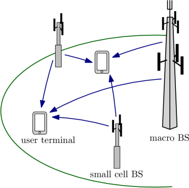
Figure 1: Small cell deployment system model.

II-B Problem Formulation

We aim at designing beamforming vectors $\{\mathbf{v}_{ik}\}_{i,k}$ to maximize the WSR under the constraints of the transmit power budget at the BSs. Mathematically, the problem reads

$$\underset{\{\mathbf{v}_{ik}\}}{\operatorname*{maximize}} \;{\textstyle\sum_{i\in\mathcal{N}}}w_{i}\log(1+\gamma_{i}(\{\mathbf{v}_{ik}\}))$$ (3a)

$$\operatorname*{subject\leavevmode\nobreak\ to} \;{\textstyle\sum_{i\in\mathcal{N}}}\mathbf{v}_{ik}^{\mbox{\scriptsize H}}\mathbf{v}_{ik}\leq P_{k},\forall k\in\mathcal{K}$$ (3b)

where $w_{i}>0$ is the priority of $\mathrm{U}_{i}$, and $P_{k}$ is the maximum transmit power available to $\mathrm{B}_{k}$. Note that the SINR in (2) is nonconvex with $\{\mathbf{v}_{ik}\}_{i,k}$, which makes problem (3) intractable [21].

II-C Centralized and Distributed Architectures of Small Cell Networks

The noncoherent JT technique can be deployed on the centralized or distributed platforms as illustrated in Fig. 2. The centralized one mainly refers to the CRANs where the baseband processing functionalities of the BSs are centralized at the BBU pool [7, 8]. It requires channel vector $\mathbf{h}_{ik}$ to be gathered at the BBU pool for all $i\in\mathcal{N},k\in\mathcal{K}$, where all beamforming vectors $\{\mathbf{v}_{ik}\}_{i\in\mathcal{N},k\in\mathcal{K}}$ are calculated. After baseband processing, the signal is sent to the BSs (remote radio head to be precise) via fronthaul links before being transmitted to users via the wireless interface. We herein focus on the performance of noncoherent JT over wireless channels. Thus, we suppose that the capacity of the fronthaul links are sufficiently large and not forming the bottleneck.

Distributed platform refers to the MEC architecture [11, 12, 10, 13, 14, 15], which is introduced to support low-latency services. Here, multiple MEC servers can be deployed across the networks to store and process data locally. In dense small cell networks, baseband processing function of one or several BSs located close to each other can be gathered at a MEC server to exploit the server’s computing capacity. A MEC server can be physically co-located with a selected BS [10]. To efficiently manage interference of dense small cells, the MEC servers should cooperate with each other in baseband processing.

We herein consider both centralized and distributed network architectures. For the latter, we suppose that there is a set of $D$ MEC servers denoted by $\mathcal{D}=\{1,...,D\}$. MEC server $d$ handles the baseband processing functionality of a set of BSs denoted by $\mathcal{K}_{d}$, $\mathcal{K}_{d}\subset\mathcal{K}$. We also suppose that each of the MEC servers can serve multiple BSs, and each of the BSs is served by only one MEC server, i.e., $|\mathcal{K}_{d}|\geq 1$, $\mathcal{K}_{d}\cap\mathcal{K}_{d^{\prime}}=\emptyset$, $\forall d\neq d^{\prime}$, and $\underset{d\in\mathcal{D}}{\cup}\mathcal{K}_{d}=\mathcal{K}$. Thus, beamforming vectors $\{\mathbf{v}_{ik}\}_{i\in\mathcal{N},k\in\mathcal{K}_{d}}$ can be locally computed at MEC server $d$ if the local CSI, i.e., $\{\mathbf{h}_{ik}\}_{i\in\mathcal{N},k\in\mathcal{K}_{d}}$, is available.

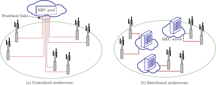
Figure 2: Centralized and distributed network architectures.

III Globally Optimal Solution to (3): A BRnB Algorithm

In this section, we develop an algorithm which globally solves (3) based on the BRnB monotonic optimization framework [30]. The purpose of finding a global solution to (3) is twofold: (i) exploring the best achievable performance of the noncoherent JT technique in small cell networks, and (ii) benchmarking against the efficient suboptimal solution to be presented. We start by rewriting (3) as

$$\underset{\{\mathbf{v}_{ik}\},\mathbf{r}\in\mathbb{R}_{+}^{N\times 1}}{\operatorname*{maximize}} \;f(\mathbf{r})\triangleq{\textstyle\sum_{i\in\mathcal{N}}}w_{i}r_{i}$$ (4a)

$$\operatorname*{subject\leavevmode\nobreak\ to} \;\log(1+\gamma_{i}(\{\mathbf{v}_{ik}\}))\geq r_{i},\forall i\in\mathcal{N}$$ (4b)

$$\;{\textstyle\sum_{i\in\mathcal{N}}}\mathbf{v}_{ik}^{\mbox{\scriptsize H}}\mathbf{v}_{ik}\leq P_{k},\forall k\in\mathcal{K}$$ (4c)

Problem (4) is the epigraph representation of (3), thus the two problems are equal in the sense of optimal solutions.

The following properties make (4) suitable for applying BRnB. First, since $w_{i}\geq 0$, objective function $f(\mathbf{r})$ is monotonically increasing with respect to $\mathbf{r}$, i.e., $f(\mathbf{r}^{\prime})\leq f(\mathbf{r})$ for all $\mathbf{r}^{\prime}\leq\mathbf{r}$ where the inequality is understood element wise. Second, let $\check{r}_{i}=0$ and $\hat{r}_{i}=\log\Bigl{(}1+\frac{\sum_{k\in\mathcal{K}}P_{k}\mathbf{h}_{ik}\mathbf{h}_{ik}^{\mbox{\scriptsize H}}}{\sigma_{i}^{2}}\Bigr{)},\,\forall i\in\mathcal{N}$, then the box $[\check{\mathbf{r}},\hat{\mathbf{r}}]$ contains all feasible points $\mathbf{r}$ in (4). Third, the set $\mathcal{S}\triangleq\{\mathbf{r}\in\mathbb{R}_{+}^{N\times 1},\eqref{eq:lograte},\eqref{eq:powerconst-2}\}$ is normal compact in $[\check{\mathbf{r}},\hat{\mathbf{r}}]$, i.e., if $\mathbf{r}^{\prime}\in\mathcal{S}$, then $[\check{\mathbf{r}},\mathbf{r}^{\prime}]\subset\mathcal{S}$.

A BRnB monotonic algorithm is an iterative procedure comprising of three main steps called branching, reduction and bounding. In what follows, we present the details of these steps customized to (4).

Let us consider iteration $t$ and define some notations. Let $\mathtt{lb}_{\mathrm{best}}$ and $\mathbf{r}_{\mathrm{best}}$ denote the current best lower bound and the feasible point achieving $\mathtt{lb}_{\mathrm{best}}$, respectively. Let $\mathcal{Q}$ be the set of candidate boxes. Let $\mathtt{ub}(R)$ denote an upper bound on $f(\mathbf{r})$ for feasible $\mathbf{r}$ in box $R$ (i.e. $\mathbf{r}\in\mathcal{S}\cap R$). The way to calculate $\mathtt{ub}(R)$ is presented in the bounding step.

Branching

In this step, a box in $\mathcal{Q}$ is picked and then divided into two smaller boxes. Specifically, let $R^{(t)}=[\underline{\mathbf{r}},\bar{\mathbf{r}}]$ denote the chosen box which has the largest upper bound compared to those in $\mathcal{Q}^{(t)}$, i.e.,

$$R^{(t)}=\underset{R\in\mathcal{Q}}{\textrm{argmax}}\;\mathtt{ub}(R).$$ (5)

Box $R^{(t)}$ is divided into two boxes $R_{1}^{(t)}=[\underline{\mathbf{r}}_{1},\bar{\mathbf{r}}_{1}]$ and $R_{2}^{(t)}=[\underline{\mathbf{r}}_{2},\bar{\mathbf{r}}_{2}]$, $R_{1}^{(t)}\cup R_{2}^{(t)}=R^{(t)}$, which are determined as

$$\underline{\mathbf{r}}_{1}=\underline{\mathbf{r}}+0.5(\bar{r}_{i}-\underline{r}_{i})\mathbf{e}_{i},\;\bar{\mathbf{r}}_{1}=\bar{\mathbf{r}},\;\underline{\mathbf{r}}_{2}=\underline{\mathbf{r}},\;\bar{\mathbf{r}}_{2}=\bar{\mathbf{r}}-0.5(\bar{r}_{i}-\underline{r}_{i})\mathbf{e}_{i}$$ (6)

where $i\in\mathcal{N}$. The upper bound of the new boxes are $\mathtt{ub}(R_{1}^{(t)})=\mathtt{ub}(R)$ , and $\mathtt{ub}(R_{2}^{(t)})=\textrm{min}\{\mathtt{ub}(R),f(\bar{\mathbf{r}}_{2})\}$ .

Remark 0.

[Branching with weighted edges] Commonly, the longest edge of $R^{(t)}$ is selected to be branched, i.e., $i=\underset{i^{\prime}\in\mathcal{N}}{\textrm{argmax}}\;(\bar{r}_{i^{\prime}}-\underline{r}_{i^{\prime}})$ [45, 46]. For the WSR problem (4), we propose the rule of choosing the longest weighted edge for branching, i.e., $i=\underset{i^{\prime}\in\mathcal{N}}{\textrm{argmax}}\;w_{i^{\prime}}(\bar{r}_{i^{\prime}}-\underline{r}_{i^{\prime}})$. The proposed rule is numerically shown to accelerate the convergence (cf. Fig. 3).

Reduction

The reduction step is to remove the parts of a box which is guaranteed not to contain an optimal solution. Let us consider the box $R=[\underline{\mathbf{r}},\bar{\mathbf{r}}]$ which has $\mathtt{ub}(R)\geq\mathtt{lb}_{\mathrm{best}}$. The reduction of $R$ is denoted by $\mathtt{red}(R)=[\underline{\mathbf{r}}^{\prime},\bar{\mathbf{r}}^{\prime}]$, where $\underline{\mathbf{r}}\leq\underline{\mathbf{r}}^{\prime}$ and $\bar{\mathbf{r}}\geq\bar{\mathbf{r}}^{\prime}$ express as

$$\underline{\mathbf{r}}^{\prime}=\bar{\mathbf{r}}-{\textstyle\sum_{i=1}^{N}}\beta_{i}(\bar{r}_{i}-\underline{r}_{i})\mathbf{e}_{i},\;\bar{\mathbf{r}}^{\prime}=\underline{\mathbf{r}}^{\prime}+{\textstyle\sum_{i=1}^{N}}\alpha_{i}(\bar{r}_{i}-\underline{r}^{\prime}_{i})\mathbf{e}_{i}$$ (7)

where

$$\begin{array}[]{c}\beta_{i}=\textrm{argmax}\{\beta|\beta\in[0,1],f(\bar{\mathbf{r}}-\beta(\bar{r}_{i}-\underline{r}_{i})\mathbf{e}_{i})\geq\mathtt{lb}_{\mathrm{best}}\}\\ \alpha_{i}=\textrm{argmax}\{\alpha|\alpha\in[0,1],f(\underline{\mathbf{r}}^{\prime}+\alpha(\bar{r}_{i}-\underline{r}^{\prime}_{i})\mathbf{e}_{i})\leq\mathtt{ub}(R)\}.\end{array}$$ (8)

It is guaranteed that any optimal solution contained in $R$ is in $\mathtt{red}(R)$. Indeed, with the $\{\alpha_{i}\}$ and $\{\beta_{i}\}$ in (8), we have $f(\underline{\mathbf{r}}^{\prime})\leq\mathtt{lb}_{\mathrm{best}}$ and $f(\bar{\mathbf{r}}^{\prime})\geq\mathtt{ub}(R)$. This means only the points $\mathbf{r}\in R$ with $f(\mathbf{r})<\mathtt{lb}_{\mathrm{best}}$ or $f(\mathbf{r})>\mathtt{ub}(R)$ are removed. In fact, (8) can be rewritten in the following closed-form expressions

$$\beta_{i}=\textrm{min}\Bigl{\{}1,\frac{f(\bar{\mathbf{r}})-\mathtt{lb}_{\mathrm{best}}}{w_{i}(\bar{r}_{i}-\underline{r}_{i})}\Bigr{\}},\,\alpha_{i}=\textrm{min}\Bigl{\{}1,\frac{\mathtt{ub}(R)-f(\underline{\mathbf{r}}^{\prime})}{w_{i}(\bar{r}_{i}-\underline{r}^{\prime}_{i})}\Bigr{\}}.$$

Bounding

This operation is to improve $\mathtt{lb}_{\mathrm{best}}$ and the upper bound of a box, from which the boxes containing no feasible point whose objective value is larger than the current $\mathtt{lb}_{\mathrm{best}}$ are removed. Let us consider the box $R=[\underline{\mathbf{r}},\bar{\mathbf{r}}]$ where $\underline{\mathbf{r}}$ is feasible (otherwise, $R$ does not contain any feasible point, and thus should be removed). Let $\boldsymbol{\phi}=\frac{\bar{\mathbf{r}}-\underline{\mathbf{r}}}{||\bar{\mathbf{r}}-\underline{\mathbf{r}}||_{2}}$, $\delta_{\mathrm{low}}=\textrm{argmax}\{\delta|(\underline{\mathbf{r}}+\delta\boldsymbol{\phi})\in\mathcal{S}\}$, and $\delta_{\mathrm{up}}=\textrm{argmin}\{\delta|(\underline{\mathbf{r}}+\delta\boldsymbol{\phi})\in[\check{\mathbf{r}},\hat{\mathbf{r}}]\setminus\mathcal{S}\}$. Clearly, the best objective value achieved by the feasible points in $R$ lies in the segment $[f(\underline{\mathbf{r}}+\delta_{\mathrm{low}}\boldsymbol{\phi}),f(\underline{\mathbf{r}}+\delta_{\mathrm{up}}\boldsymbol{\phi})]$. Thus, we can update $\mathtt{lb}_{\mathrm{best}}$ and $\mathtt{ub}(R)$ as: $\mathtt{lb}_{\mathrm{best}}=\textrm{max}\{f(\underline{\mathbf{r}}+\delta_{\mathrm{low}}\boldsymbol{\phi}),\mathtt{lb}_{\mathrm{best}}\}$ and $\mathtt{ub}(R)=\textrm{min}\{\textrm{max}\{f(\bar{\mathbf{r}}-(\bar{r}_{i}-\underline{r}_{i}-\delta_{\mathrm{up}}\phi_{i})\mathbf{e}_{i}|i\in\mathcal{N}\},\mathtt{ub}(R)\}$. The values of $\delta_{\mathrm{low}}$ and $\delta_{\mathrm{up}}$ can be determined by the bisection algorithm over the interval $[0,||\bar{\mathbf{r}}-\underline{\mathbf{r}}||_{2}]$.

Checking Feasibility

From the above discussions, it becomes apparent that checking whether a given point is feasible or not plays the key role in bounding. Given $\mathbf{r}$, the feasibility problem is given by

$$\tilde{\mathcal{S}}(\mathbf{r})=\mathrm{find} \;\{\mathbf{v}_{ik}\}$$ (9a)

$$\operatorname*{subject\leavevmode\nobreak\ to} \;\frac{\sum_{k\in\mathcal{K}}|\mathbf{h}_{ik}\mathbf{v}_{ik}|^{2}}{\sum_{k\in\mathcal{K}}\sum_{\begin{subarray}{c}j\in\mathcal{N}\setminus\{i\}\end{subarray}}|\mathbf{h}_{ik}\mathbf{v}_{jk}|^{2}+\sigma_{i}^{2}}\geq\tilde{r}_{i},\forall i\in\mathcal{N}$$ (9b)

$$\;{\textstyle\sum_{i\in\mathcal{N}}}\mathbf{v}_{ik}^{\mbox{\scriptsize H}}\mathbf{v}_{ik}\leq P_{k},\forall k\in\mathcal{K}$$ (9c)

where $\tilde{r}_{i}=\exp(r_{i})-1$. The feasible set in (9) is nonconvex due to (9b). Different from the coherent JT, using the trick of a phase rotation here does not lead to a tractable formulation due to the sum of quadratic functions at numerator in (9b) [45]. However, problem (9) can be solved exactly using semidefinite relaxation (SDR). In particular, let us write the SDR of (9) as

$$\tilde{\mathcal{S}}_{\mathrm{SD}}(\mathbf{r})=\mathrm{find} \;\{\mathbf{V}_{ik}\}$$ (10a)

$$\operatorname*{subject\leavevmode\nobreak\ to} \;{\textstyle\sum_{k\in\mathcal{K}}}\mathbf{h}_{ik}\mathbf{V}_{ik}\mathbf{h}_{ik}^{\mbox{\scriptsize H}}\geq\tilde{r}_{i}{\textstyle\sum_{k\in\mathcal{K}}\sum_{\begin{subarray}{c}j\in\mathcal{N}\setminus\{i\}\end{subarray}}}\mathbf{h}_{ik}\mathbf{V}_{jk}\mathbf{h}_{ik}^{\mbox{\scriptsize H}}+\tilde{r}_{i}\sigma_{i}^{2},\forall i\in\mathcal{N}$$ (10b)

$$\;{\textstyle\sum_{i\in\mathcal{N}}}\operatorname{tr}(\mathbf{V}_{ik})\leq P_{k},\forall k\in\mathcal{K},\;\mathbf{V}_{ik}\in\mathbb{S}_{+}^{M_{k}},\forall i\in\mathcal{N},\forall k\in\mathcal{K}.$$ (10c)

The relationship between (9) and (10) in terms of feasibility is stated in the following lemma.

Lemma 2.

For a given point $\mathbf{r}$, the set $\tilde{\mathcal{S}}(\mathbf{r})$ is nonempty if and only if $\tilde{\mathcal{S}}_{\mathrm{SD}}(\mathbf{r})$ is nonempty.

Proof:

The proof is given in Appendix A-A. ∎

The result in Lemma 2 means that the feasibility of some point $\mathbf{r}$ can be justified via (10).

The Globally Optimal Algorithm

The proposed BRnB algorithm for solving (3) is outlined in Algorithm 1. Line 3 is branching, line 4 is reduction, and lines 5-7 are bounding, as explained above. At the initial stage (line 1), we can randomly generate $\{\mathbf{v}_{ik}\}$ such that (3b) is satisfied, and then determine $\mathbf{r}_{\mathrm{best}}$ by letting (4b) hold with equality. Notation $\mathtt{UB}$ denotes the current largest upper bound (of the boxes in $\mathcal{Q}$). Removing boxes that do not contain any optimal solution is shown in line 8. The stopping criterion in line 10 ensures that the output $\mathtt{lb}_{\mathrm{best}}$ is not lower than $100(1-\epsilon)\%$ of the optimality. To determine beamforming vectors $\{\mathbf{v}_{ik}^{\star}\}$ achieving $\mathbf{r}_{\mathrm{best}}$, i.e., line 11, we first solve problem

$$\underset{\{\mathbf{V}_{ik}\}}{\operatorname*{minimize}}\;{\textstyle\sum_{i\in\mathcal{N}}\sum_{k\in\mathcal{K}}}\operatorname{tr}(\mathbf{V}_{ik})\;\operatorname*{subject\leavevmode\nobreak\ to}\textrm{ \{\eqref{eq:relaxation1}, \eqref{eq:relaxation2}\}}$$ (11)

and denote the obtained solution by $\{\mathbf{V}^{\prime}_{ik}\}$. If $\mathrm{rank}(\mathbf{V}^{\prime}_{ik})\leq 1$, we extract $\mathbf{v}_{ik}^{\star}$ via the eigenvalue decomposition of $\mathbf{V}^{\prime}_{ik}$. Otherwise, $\mathbf{v}_{ik}^{\star}$ can be found as the solution to the following CQP derived from (32) (see Appendix A-A)

$$\underset{||\mathbf{v}||_{2}^{2}\leq\operatorname{tr}(\mathbf{V}^{\prime}_{ik})}{\operatorname*{maximize}}\;\mathrm{Re}\{\mathbf{h}_{ik}\mathbf{v}\}\;\operatorname*{subject\leavevmode\nobreak\ to}\;\mathbf{v}^{\mbox{\scriptsize H}}\mathbf{h}_{jk}^{\mbox{\scriptsize H}}\mathbf{h}_{jk}\mathbf{v}\leq\mathbf{h}_{jk}\mathbf{V}^{\prime}_{ik}\mathbf{h}_{jk}^{\mbox{\scriptsize H}},\forall j\neq i.$$ (12)

We now discuss the optimality of Algorithm 1. In particular, let us denote by $f_{\mathrm{opt}}$ the optimal objective value. Then we have the following lemma.

Lemma 3.

Given any $\varepsilon>0$, Algorithm 1 guarantees to achieve $\mathtt{UB}-\mathtt{lb}_{\mathrm{best}}<\varepsilon$ where $f_{\mathrm{opt}}\in[\mathtt{lb}_{\mathrm{best}},\mathtt{UB}]$ in a finite number of iterations.

Proof:

A proof is provided in Appendix A-B. ∎

Since $\mathbf{r}_{\mathrm{best}}$ is feasible, the lemma means that we can find an $\varepsilon$-approximate optimal solution, i.e. $f_{\mathrm{opt}}-f(\mathbf{r}_{\mathrm{best}})<\varepsilon$, for any $\varepsilon>0$ after a finite number of iterations.

The computational complexity of each iteration in Algorithm 1 is mainly incurred by solving feasibility problems (10) at the bounding process. More explicitly, problem (10) contains $2N\sum_{k}M_{k}^{2}$ real variables, $(N+K)$ constraints in size 1, and $N$ constraints in size $\sum_{k}2M_{k}$ for each $k$. So, the worst-case of computational cost for solving (10) is $\mathcal{O}(\sqrt{K+N(1+2\sum_{k}M_{k})}\linebreak 4N^{2}(\sum_{k}M_{k}^{2})^{2}(K+N(1+4\sum_{k}M_{k}^{2})))$ [47]. The number of problems needed to be solved depends on the bisection accuracy, denoted by $\epsilon_{\textrm{bi}}$, of determining $\delta_{\mathrm{low}}$ and $\delta_{\mathrm{up}}$, which is $\mathcal{O}(\log_{2}(1/\epsilon_{\textrm{bi}}))$.

Algorithm 1 A Branch Reduce and Bound Algorithm to Globally Solve (3)

1:  Initialization: set $t\coloneqq 1$, $\mathcal{Q}\coloneqq[\check{\mathbf{r}},\hat{\mathbf{r}}]$, $\mathtt{UB}\coloneqq f(\hat{\mathbf{r}})$. Set initial $\mathbf{r}_{\mathrm{best}}$ and $\mathtt{lb}_{\mathrm{best}}=f(\mathbf{r}_{\mathrm{best}})$. Given accuracy parameter $\epsilon$.

2:  repeat

3:     Select $R^{(t)}$ as (5), then branch $R^{(t)}$ into $R_{1}^{(t)}$ and $R_{2}^{(t)}$ as (6). $\mathcal{Q}\coloneqq\mathcal{Q}\setminus R^{(t)}$.

4:     if $\mathtt{ub}(R_{m}^{(t)})\geq\mathtt{lb}_{\mathrm{best}}$ where $m\in\{1,2\}$, then determine $\mathtt{red}(R_{m}^{(t)})$ and update $\mathcal{Q}\coloneqq\mathcal{Q}\cup\mathtt{red}(R_{m}^{(t)})$ end.

5:     if $\mathtt{red}(R_{1}^{(t)})=[\underline{\mathbf{r}}_{1}^{\prime},\bar{\mathbf{r}}_{1}^{\prime}]$ contains feasible points (check feasibility of $\underline{\mathbf{r}}_{1}^{\prime}$) then

6:      determine $\boldsymbol{\phi}=\frac{\bar{\mathbf{r}}_{1}^{\prime}-\underline{\mathbf{r}}_{1}^{\prime}}{||\bar{\mathbf{r}}_{1}^{\prime}-\underline{\mathbf{r}}_{1}^{\prime}||_{2}}$, $\delta_{\mathrm{low}}$ and $\delta_{\mathrm{up}}$, and update $\mathtt{lb}_{\mathrm{best}}$ , $\mathbf{r}_{\mathrm{best}}$, and $\mathtt{ub}(\mathtt{red}(R_{1}^{(t)}))$

7:     else set $\mathtt{ub}(\mathtt{red}(R_{1}^{(t)}))=0$ end.

8:     Update $\mathcal{Q}\coloneqq\mathcal{Q}\setminus\{R|\mathtt{ub}(R)<\mathtt{lb}_{\mathrm{best}}\}$.

9:     Update $\mathtt{UB}\coloneqq\textrm{max}\{\mathtt{ub}(R)|R\in\mathcal{Q}\}$, $t:=t+1$.

10:  until $\frac{\mathtt{UB}-\mathtt{lb}_{\mathrm{best}}}{\mathtt{lb}_{\mathrm{best}}}\leq\epsilon$

11:  Determine beamforming vectors $\{\mathbf{v}_{ik}^{\star}\}$ which achieve $\mathbf{r}_{\mathrm{best}}$.

12:  Output: $\mathbf{r}_{\mathrm{best}}$, $\mathtt{lb}_{\mathrm{best}}$, and $\{\mathbf{v}_{ik}^{\star}\}$.

IV Efficient Solution to (3): An InAp-based Algorithm

The globally optimal algorithm presented in the previous section comes at a high computational cost, and might be unsuitable for a real-time practical implementation. In this section, we present a fast converging and low-complexity solution to (3) based on the InAp framework, which was inspired by our earlier work in [44]. To do so, we first transform (3) into an equivalent form where convexity is easily justified as follows

$$\underset{\{\mathbf{v}_{ik}\},\{\mu_{i}\}}{\operatorname*{maximize}} \;{\textstyle\sum_{i\in\mathcal{N}}}w_{i}\log(1+\mu_{i})$$ (13a)

$$\operatorname*{subject\leavevmode\nobreak\ to} \;\frac{{\textstyle\sum_{k\in\mathcal{K}}}|\mathbf{h}_{ik}\mathbf{v}_{ik}|^{2}}{{\textstyle\sum_{k\in\mathcal{K}}\sum_{\begin{subarray}{c}j\in\mathcal{N}\setminus\{i\}\end{subarray}}}|\mathbf{h}_{ik}\mathbf{v}_{jk}|^{2}+\sigma_{i}^{2}}\geq\mu_{i},\forall i\in\mathcal{N},$$ (13b)

$$\;{\textstyle\sum_{i\in\mathcal{N}}}\mathbf{v}_{ik}^{\mbox{\scriptsize H}}\mathbf{v}_{ik}\leq P_{k},\forall k\in\mathcal{K}$$ (13c)

where $\{\mu_{i}\geq 0\}$ are newly introduced variables.

Lemma 4.

Let $(\{\mathbf{v}_{ik}^{\star}\},\{\mu_{i}^{\star}\})$ be an optimal solution to (13), then $\{\mathbf{v}_{ik}^{\star}\}$ is an optimal solution to (3). Conversely, let $\{\mathbf{v}_{ik}^{\ast}\}$ be an optimal solution to (3), then $(\{\mathbf{v}_{ik}^{\ast}\},\{\gamma_{i}(\{\mathbf{v}_{ik}^{\ast}\})\})$ is an optimal solution to (13). Moreover, the two problems have the same optimal objective value.

Proof:

A proof is provided in Appendix A-C. ∎

It is clear that the nonconvexity of (4) is due to (13b), which can be equivalently rewritten as

$$\eqref{eq:snrconstr}\Leftrightarrow\begin{cases}{\textstyle\sum_{k\in\mathcal{K}}}|\mathbf{h}_{ik}\mathbf{v}_{ik}|^{2}/u_{i}\geq\mu_{i}\\ {\textstyle\sum_{k\in\mathcal{K}}\sum_{\begin{subarray}{c}j\in\mathcal{N}\setminus\{i\}\end{subarray}}}|\mathbf{h}_{ik}\mathbf{v}_{jk}|^{2}+\sigma_{i}^{2}\leq u_{i}\end{cases}$$ (14)

where $\{u_{i}>0\}$ are slack variables. Note that the quadratic-over-linear function is convex with the involved variables. We introduce $\{u_{i}\}$ to avoid the function $\sum_{k\in\mathcal{K}}|\mathbf{h}_{ik}\mathbf{v}_{ik}|^{2}/\mu_{i}$, which might lead to numerical problems, since $\mu_{i}$ could be zero. In light of the InAp approach, we use a first order approximation as a convex lower bound to derive an approximate convex problem. More explicitly, let $(\{\mathbf{v}_{i}^{(t)}\},\{\mu_{i}^{(t)}\},\{u_{i}^{(t)}\})$ be a feasible point, then the approximate problem is

$$\underset{\{\mathbf{v}_{ik}\},\{\mu_{i}\},\{u_{i}\}}{\operatorname*{maximize}} \;{\textstyle\sum_{i\in\mathcal{N}}}w_{i}\log(1+\mu_{i})$$ (15a)

$$\operatorname*{subject\leavevmode\nobreak\ to} \;{\textstyle\sum_{k\in\mathcal{K}}}(\mathrm{Re}\{\mathbf{g}_{ik}^{(t)}\mathbf{v}_{ik}\}-A_{ik}^{(t)}u_{i})\geq\mu_{i},\forall i\in\mathcal{N},$$ (15b)

$$\;{\displaystyle{\textstyle\sum_{k\in\mathcal{K}}\sum_{\begin{subarray}{c}j\in\mathcal{N}\setminus\{i\}\end{subarray}}}}|\mathbf{h}_{ik}\mathbf{v}_{jk}|^{2}+\sigma_{i}^{2}\leq u_{i},\forall i\in\mathcal{N},$$ (15c)

$$\;{\textstyle\sum_{i\in\mathcal{N}}}\mathbf{v}_{ik}^{\mbox{\scriptsize H}}\mathbf{v}_{ik}\leq P_{k},\forall k\in\mathcal{K}$$ (15d)

where $\mathbf{g}_{ik}^{(t)}=(2/u_{i}^{(t)})(\mathbf{v}_{ik}^{(t)})^{\mbox{\scriptsize H}}\mathbf{h}_{ik}^{\mbox{\scriptsize H}}\mathbf{h}_{ik}$ and $A_{ik}^{(t)}=(|\mathbf{h}_{ik}\mathbf{v}_{ik}^{(t)}|/u_{i}^{(t)})^{2}$.

CQP-Based Approximation

Since $w_{i}$, $i\in\mathcal{N}$, is generally different, problem (15) containing a mix of exponential and second-order cones is normally treated as a generic convex program. The efficiency of modern convex solvers in solving these generic programs is far less than in solving more standard ones. This motivates us to present a quadratic approximation of the objective to obtain a CQP approximate problem of (15). We achieve this by using a lower bound of the logarithm function given as

$$\log(1+\mu_{i})\geq\log(1+\mu_{i}^{(t)})+2-2\sqrt{(1+\mu_{i}^{(t)})/(1+\mu_{i})}.$$ (16)

The validity of the bound according to the InAp principles is justified in our recent work [48, Sec. III-E]. Next, by introducing new variables $\{\delta_{i}\}$ and $\{\pi_{i}\}$, we arrive at the following CQP approximation

$$\underset{\mathbf{x}}{\operatorname*{minimize}} \;{\textstyle\sum_{i\in\mathcal{N}}}\tilde{w}_{i}^{(t)}\pi_{i}$$ (17a)

$$\operatorname*{subject\leavevmode\nobreak\ to} \;\parallel[2,(\pi_{i}-\delta_{i})]\parallel_{2}\leq(\pi_{i}+\delta_{i}),1+\mu_{i}\geq\delta_{i}^{2},\delta_{i}\geq 1,\forall i\in\mathcal{N},$$ (17b)

$$\;\eqref{eq:snrconstr-2},\eqref{eq:interf},\eqref{eq:powerconst-1-2}$$ (17c)

where $\tilde{w}_{i}^{(t)}=w_{i}\sqrt{1+\mu_{i}^{(t)}}$, $\mathbf{x}\triangleq\{\{\mathbf{v}_{ik}\},\{\mu_{i}\},\{u_{i}\},\{\delta_{i}\},\{\pi_{i}\}\}$.

Algorithm and Convergence

The InAp-based iterative procedure is outlined in Algorithm 2, which starts with a random initial point (Step 1). In each iteration, a CQP is solved (Step 3) and the feasible point is updated (Step 13). Successively solving (17) and updating $(\{\mathbf{v}_{i}^{(t)}\},\{\mu_{i}^{(t)}\},\{u_{i}^{(t)}\})$ by the optimal solution of (17), we obtain the objective sequence $\{\sum_{i\in\mathcal{N}}w_{i}\log(1+\mu_{i}^{(t)})\}_{t=0}^{\infty}$ which is guaranteed to converge as stated in the following lemma.

Lemma 5.

Any sequence $\{\sum_{i\in\mathcal{N}}w_{i}\log(1+\mu_{i}^{(t)})\}_{t=0}^{\infty}$ produced by Algorithm 2 is monotonically increasing and converges.

Proof:

A proof is provided in Appendix A-D. ∎

Algorithm 2 An InAp Algorithm to Efficiently Solve (3)

1:  Initialization: Set small $\epsilon_{\mathrm{IA}}$, set $t\coloneqq 0$, choose initial $(\{\mathbf{v}_{i}^{(0)}\},\{\mu_{i}^{(0)}\},\{u_{i}^{(0)}\})$.

2:  repeat

3:     Solve (17), and denote the optimal solution by $(\{\mathbf{v}_{i}^{\ast}\},\{\mu_{i}^{\ast}\},\{u_{i}^{\ast}\})$

4:     Update $(\{\mathbf{v}_{i}^{(t+1)}\},\{\mu_{i}^{(t+1)}\},\{u_{i}^{(t+1)}\}):=(\{\mathbf{v}_{i}^{\ast}\},\{\mu_{i}^{\ast}\},\{u_{i}^{\ast}\})$

5:     Update $t:=t+1$

6:  until Convergence on objective value

7:  Output: $\{\mathbf{v}_{i}^{(t)}\}$

Computational Complexity

The computational complexity of the algorithm depends on the arithmetical cost of solving approximate problem (17) in each iteration. Problem (17) includes $2N(2+M)$ real variables where $M=\sum_{k\in\mathcal{K}}M_{k}$, $2N$ constraints in size 3, $2N$ constraints in size 1, $N$ constraints in size $K(N-1)+N+2$ , and one constraint in size $2M_{k}+1$ for BS $k$, $\forall k\in\mathcal{K}$. Hence, the worst-case computational cost of using a general interior point method for solving (17) is $\mathcal{O}(\sqrt{1+5N+K}4N^{2}(2+M)^{2}(N^{2}(K+1)+N(10-K)+2M+K))$ [47].

Remark 0.

[A first-order solution to (3)] We have introduced a few slack variables to achieve a CQP approximation. This maneuver certainly increases the complexity of the problem and may question the efficacy of the proposed iterative solution. This concern is especially relevant as the feasible set of (3) is expressed as a system of separable quadratic convex constraints. Thus it is apparently appealing to approximate the objective of (3) by means of a first-order optimization method. In this way, the resulting program in each iteration has low complexity compared to (17). One of the first-order methods widely used for a nonconvex problem such as (3) is the conditional gradient technique (a.k.a. the Frank-Wolfe method) that have received significant interest recently [49, 50, 51]. In Appendix B we show how a Frank-Wolfe (FW) type algorithm can be derived to solve (3), where the linear optimization oracle at each iteration admits a closed-form expression. While looking very attractive from a per-iteration cost viewpoint, FW type methods in general converge very slowly, i.e., they need a very large number of iterations to produce a high-accuracy solution. As a consequence, the actual run time of the FW type algorithm is much higher than our proposed solution presented in Algorithm 2. We provide numerical examples to demonstrate this point in Fig. 5.

V Distributed Implementation: A Combination of InAp and ADMM

In this section, we develop a decentralized algorithm implementing the InAp-based solution where beamforming vectors are calculated locally at the MEC servers using local CSI. The approach is to use the ADMM to solve the convex approximation subproblem (17), in which (17) is converted to an equivalent transformation so that the ADMM procedure can be distributively implemented.

V-A Distributed Formulation

We first rearrange (17) according to the MEC servers as

$$\underset{\mathbf{x}}{\operatorname*{minimize}} \;{\textstyle\sum_{i\in\mathcal{N}}}\tilde{w}_{i}^{(t)}\pi_{i}$$ (18a)

$$\operatorname*{subject\leavevmode\nobreak\ to} \;\parallel[2,(\pi_{i}-\delta_{i})]\parallel_{2}\leq(\pi_{i}+\delta_{i}),1+\mu_{i}\geq\delta_{i}^{2},\delta_{i}\geq 1,\forall i\in\mathcal{N},$$ (18b)

$$\;{\textstyle\sum_{d\in\mathcal{D}}\sum_{k\in\mathcal{K}_{d}}}(\mathrm{Re}\{\mathbf{g}_{ik}^{(t)}\mathbf{v}_{ik}\}-A_{ik}^{(t)}u_{i})\geq\mu_{i},\forall i\in\mathcal{N},$$ (18c)

$$\;{\textstyle\sum_{d\in\mathcal{D}}\sum_{k\in\mathcal{K}_{d}}\sum_{\begin{subarray}{c}j\in\mathcal{N}\setminus\{i\}\end{subarray}}}|\mathbf{h}_{ik}\mathbf{v}_{jk}|^{2}+\sigma_{i}^{2}\leq u_{i},\forall i\in\mathcal{N},$$ (18d)

$$\;{\textstyle\sum_{i\in\mathcal{N}}}\mathbf{v}_{ik}^{\mbox{\scriptsize H}}\mathbf{v}_{ik}\leq P_{k},\forall k\in\mathcal{K}.$$ (18e)

We observe that (18c) and (18d) are the coupling constraints. Thus, we introduce local and global variables so that these constraints are decoupled among the MEC servers. In particular, we equivalently rewrite (18) into the following form

$$\underset{\begin{subarray}{c}\{\mathbf{v}_{ik}\},\{\mu_{i}\},\{u_{i}\},\{\delta_{i}\},\\ \{\pi_{i}\},\{\hat{q}_{ik}\},\{\tilde{q}_{ik}\},\{q_{ik}\},\\ \{\hat{y}_{ik}\},\{\tilde{y}_{ik}\},\{y_{ik}\}\end{subarray}}{\operatorname*{minimize}} \;{\textstyle\sum_{i\in\mathcal{N}}}\tilde{w}_{i}^{(t)}\pi_{i}$$ (19a)

$$\operatorname*{subject\leavevmode\nobreak\ to} \;{\textstyle\sum_{k\in\mathcal{K}_{1}}}\mathrm{Re}\{\mathbf{g}_{ik}^{(t)}\mathbf{v}_{ik}\}-\left({\textstyle\sum_{k\in\mathcal{K}_{1}}}A_{ik}^{(t)}+{\textstyle\sum_{d\in\bar{\mathcal{D}}}\sum_{k\in\mathcal{K}_{d}}}A_{ik}^{(t)}\right)u_{i}$$

$$\;\hskip 199.16928pt+{\textstyle\sum_{d\in\bar{\mathcal{D}}}}\tilde{y}_{id}\geq\mu_{i},\forall i\in\mathcal{N},$$ (19b)

$$\;{\textstyle\sum_{k\in\mathcal{K}_{d}}}\mathrm{Re}\{\mathbf{g}_{ik}^{(t)}\mathbf{v}_{ik}\}\geq\hat{y}_{id},\forall i\in\mathcal{N},d\in\bar{\mathcal{D}}$$ (19c)

$$\;{\textstyle\sum_{k\in\mathcal{K}_{1}}\sum_{\begin{subarray}{c}j\in\mathcal{N}\setminus\{i\}\end{subarray}}}|\mathbf{h}_{ik}\mathbf{v}_{jk}|^{2}+{\textstyle\sum_{d\in\bar{\mathcal{D}}}}\tilde{q}_{id}+\sigma_{i}^{2}\leq u_{i},\forall i\in\mathcal{N},$$ (19d)

$$\;{\textstyle\sum_{k\in\mathcal{K}_{d}}\sum_{\begin{subarray}{c}j\in\mathcal{N}\setminus\{i\}\end{subarray}}}|\mathbf{h}_{ik}\mathbf{v}_{jk}|^{2}\leq\hat{q}_{id},\forall i\in\mathcal{N},d\in\bar{\mathcal{D}}$$ (19e)

$$\;\hat{q}_{id}=q_{id},\hat{y}_{id}=y_{id},\forall i\in\mathcal{N},\forall d\in\bar{\mathcal{D}}$$ (19f)

$$\;\tilde{q}_{id}=q_{id},\tilde{y}_{ik}=y_{id},\forall i\in\mathcal{N},\forall d\in\bar{\mathcal{D}}$$ (19g)

$$\;\eqref{eq:powerref},\eqref{eq:log_appr-1}$$ (19h)

where $\bar{\mathcal{D}}=\mathcal{D}\setminus\{1\}$, and $\{\hat{q}_{id}\}$, $\{\tilde{q}_{id}\}$, $\{q_{id}\}$, $\{\hat{y}_{id}\}$, $\{\tilde{y}_{id}\}$ and $\{y_{id}\}$ are newly introduced variables for decomposing (18c) and (18d) into constraints which will be handled locally at the MEC servers; constraints (19f) and (19g) ensure the agreement of the local variables $\{\hat{q}_{id}\}$ and $\{\tilde{q}_{id}\}$, and $\{\hat{y}_{id}\}$ and $\{\tilde{y}_{id}\}$.

Lemma 7.

Let $(\mathbf{x}^{\star},\{\hat{q}_{id}^{\star}\},\{\tilde{q}_{id}^{\star}\},\{q_{id}^{\star}\},\{\hat{y}_{id}^{\star}\},\{\tilde{y}_{id}^{\star}\},\{y_{id}^{\star}\})$ be an optimal solution to (19), then $\mathbf{x}^{\star}$ is an optimal solution to (18). Conversely, let $\mathbf{x}^{\ast}$ be an optimal solution to (18), then $(\mathbf{x}^{\ast},\{\hat{q}_{id}^{\ast}\},\{\tilde{q}_{id}^{\ast}\},\{q_{id}^{\ast}\},\{\hat{y}_{id}^{\ast}\},\{\tilde{y}_{id}^{\ast}\},\{y_{id}^{\ast}\})$ where $\tilde{q}_{id}^{\ast}=q_{id}^{\ast}=\hat{q}_{id}^{\ast}={\textstyle\sum_{k\in\mathcal{K}_{d}}\sum_{\begin{subarray}{c}j\in\mathcal{N}\setminus\{i\}\end{subarray}}}|\mathbf{h}_{ik}\mathbf{v}_{jk}^{\ast}|^{2}$ and $\tilde{y}_{id}^{\ast}=y_{id}^{\ast}=\hat{y}_{id}^{\ast}={\textstyle\sum_{k\in\mathcal{K}_{d}}}\mathrm{Re}\{\mathbf{g}_{ik}^{(t)}\mathbf{v}_{ik}^{\ast}\}$, $\forall i\in\mathcal{N},d\in\bar{\mathcal{D}}$, is an optimal solution to (19).

Proof:

The lemma can be proved by using the similar approach to that of Lemma 4. The detail is omitted for the sake of brevity. ∎

We now rewrite (19) in a more compact form. Without loss of generality, we assume that macro BS is controlled by MEC server 1 and $\bar{\mathcal{D}}=\mathcal{D}\setminus\{1\}$. For notational convenience, let us denote by $\tilde{\mathbf{x}}\triangleq\{\{\mathbf{v}_{ik}\}_{i\in\mathcal{N},k\in\mathcal{K}_{1}},\{\mu_{i}\}_{i\in\mathcal{N}},\{u_{i}\}_{i\in\mathcal{N}},\{\delta_{i}\}_{i\in\mathcal{N}},\{\pi_{i}\}_{i\in\mathcal{N}},\{\tilde{q}_{id}\}_{i\in\mathcal{N},d\in\bar{\mathcal{D}}},\{\tilde{y}_{id}\}_{i\in\mathcal{N},d\in\bar{\mathcal{D}}}\}$ the local variables at MEC server 1, and define its local feasible set as

$$\tilde{\mathcal{S}} \triangleq\{\tilde{\mathbf{x}}|\eqref{eq:snrconstr-1-1},\eqref{eq:snrcontr2},\eqref{eq:log_appr},{\textstyle\sum_{i\in\mathcal{N}}}\mathbf{v}_{ik}^{\mbox{\scriptsize H}}\mathbf{v}_{ik}\leq P_{k},\forall k\in\mathcal{K}_{1}\}.$$ (20)

Similarly, let us denote by $\hat{\mathbf{x}}_{d}\triangleq\{\{\mathbf{v}_{ik}\}_{i\in\mathcal{N},k\in\mathcal{K}_{d}},\{\hat{q}_{id}\}_{i\in\mathcal{N}},\{\hat{y}_{id}\}_{i\in\mathcal{N}}\}$ the local variables at MEC server $d$, $d\in\bar{\mathcal{D}}$, and define its local feasible set as

$$\hat{\mathcal{S}}_{d}=\{\hat{\mathbf{x}}_{d}|{\textstyle\sum_{k\in\mathcal{K}_{d}}}\mathrm{Re}\{\mathbf{g}_{ik}^{(t)}\mathbf{v}_{ik}\}\geq\hat{y}_{id},\forall i\in\mathcal{N},{\textstyle\sum_{k\in\mathcal{K}_{d}}\sum_{\begin{subarray}{c}j\in\mathcal{N}\setminus\{i\}\end{subarray}}}|\mathbf{h}_{ik}\mathbf{v}_{jk}|^{2}\leq\hat{q}_{id},\forall i\in\mathcal{N},\\ {\textstyle\sum_{i\in\mathcal{N}}}\mathbf{v}_{ik}^{\mbox{\scriptsize H}}\mathbf{v}_{ik}\leq P_{k},\forall k\in\mathcal{K}_{d}\}.$$ (21)

With these notations, we can rewrite (19) as

$$\underset{\begin{subarray}{c}\{\tilde{\mathbf{x}}\in\tilde{\mathcal{S}}\},\{\hat{\mathbf{x}}_{d}\in\hat{\mathcal{S}}_{d}\}_{d\in\bar{\mathcal{D}}}\\ \{q_{id}\}_{i\in\mathcal{N},d\in\bar{\mathcal{D}}},\{y_{id}\}_{i\in\mathcal{N},d\in\bar{\mathcal{D}}}\end{subarray}}{\operatorname*{minimize}} \;{\textstyle\sum_{i\in\mathcal{N}}}\tilde{w}_{i}^{(t)}\pi_{i}$$ (22a)

$$\operatorname*{subject\leavevmode\nobreak\ to} \;\tilde{\boldsymbol{\pi}}=\tilde{\boldsymbol{\phi}},\hat{\boldsymbol{\pi}}_{d}=\hat{\boldsymbol{\phi}}_{d},\forall d\in\bar{\mathcal{D}}$$ (22b)

where $\tilde{\boldsymbol{\pi}}\triangleq\{\{\tilde{q}_{id}\}_{i\in\mathcal{N},d\in\bar{\mathcal{D}}},\{\tilde{y}_{id}\}_{i\in\mathcal{N},d\in\bar{\mathcal{D}}}\}$, $\hat{\boldsymbol{\pi}}_{d}\triangleq\{\{\hat{q}_{id}\}_{i\in\mathcal{N}},\{\tilde{y}_{id}\}_{i\in\mathcal{N}}\}$; $\tilde{\boldsymbol{\phi}}$ and $\hat{\boldsymbol{\phi}}_{d}$ are the rearranged vectors from the same set of global variables $(\{q_{id}\}_{i\in\mathcal{N},d\in\bar{\mathcal{D}}},\{y_{id}\}_{i\in\mathcal{N},d\in\bar{\mathcal{D}}})$.

Now, it can be seen that (22) is in the form of consensus problem which can be solved using the ADMM [35]. We have the augmented Lagrangian function of (22) given by

$$\mathfrak{L}(\{\tilde{\mathbf{x}}\},\{\hat{\mathbf{x}}_{d}\},\{q_{id}\},\{y_{id}\};\{\boldsymbol{\xi}\},\{\boldsymbol{\rho}_{d}\})=\Bigl{(}\boldsymbol{\xi}^{\mbox{\scriptsize T}}(\tilde{\boldsymbol{\pi}}-\tilde{\boldsymbol{\phi}})+\frac{m}{2}||\tilde{\boldsymbol{\pi}}-\tilde{\boldsymbol{\phi}}||_{2}^{2}+{\textstyle\sum_{i\in\mathcal{N}}}\tilde{w}_{i}^{(t)}\pi_{i}\Bigr{)}\\ +{\textstyle\sum_{d\in\bar{\mathcal{D}}}}\left(\boldsymbol{\rho}_{d}^{\mbox{\scriptsize T}}(\hat{\boldsymbol{\pi}}_{d}-\hat{\boldsymbol{\phi}}_{d})+\frac{m}{2}||\hat{\boldsymbol{\pi}}_{d}-\hat{\boldsymbol{\phi}}_{d}||_{2}^{2}\right)$$ (23)

where $\boldsymbol{\xi}\in\mathbb{R}^{N(D-1)\times 1}$ and $\{\boldsymbol{\rho}_{d}\}_{d\in\bar{\mathcal{D}}}$,$\boldsymbol{\rho}_{d}\in\mathbb{R}^{N\times 1}$, are the vectors of Lagrangian multipliers; $m>0$ is the penalty parameter that weighs the violation of the equality constraints. In what follows, we present the variable updates at iteration $(j+1)$ of the ADMM procedure.

V-B Variable Updates

V-B1 Update Local Variables

Let $\boldsymbol{\xi}^{(j)}$, $\tilde{\boldsymbol{\phi}}^{(j)}$, and $\{\boldsymbol{\rho}_{d}^{(j)}\}$ be the values obtained at iteration $j$. MEC server 1 updates its local variables $\tilde{\mathbf{x}}$ by solving the following CQP

$$\underset{\tilde{\mathbf{x}}\in\tilde{\mathcal{S}}}{\operatorname*{minimize}}\;(\boldsymbol{\xi}^{(j)})^{\mbox{\scriptsize T}}(\tilde{\boldsymbol{\pi}}-\tilde{\boldsymbol{\phi}}^{(j)})+\frac{m}{2}||\tilde{\boldsymbol{\pi}}-\tilde{\boldsymbol{\phi}}^{(j)}||_{2}^{2}+{\textstyle\sum_{i\in\mathcal{N}}}\tilde{w}_{i}^{(t)}\pi_{i}.$$ (24)

Also, MEC server $d$, $d\in\bar{\mathcal{D}}$, updates its local variables $\hat{\mathbf{x}}_{d}$ by solving the following quadratically constrained quadratic program (QCQP)

$$\underset{\hat{\mathbf{x}}_{d}\in\hat{\mathcal{S}}_{d}}{\operatorname*{minimize}}\;(\boldsymbol{\rho}_{d}^{(j)})^{\mbox{\scriptsize T}}(\hat{\boldsymbol{\pi}}_{d}-\hat{\boldsymbol{\phi}}_{d}^{(j)})+\frac{m}{2}||\hat{\boldsymbol{\pi}}_{d}-\hat{\boldsymbol{\phi}}_{d}^{(j)}||_{2}^{2}.$$ (25)

V-B2 Update Global Variables

The global variables $\{q_{id}\}$ and $\{y_{id}\}$ are updated via finding the minimum of the following quadratic function derived from (23)

$$G^{(j)}(\{q_{id}\},\{y_{id}\})\triangleq{\textstyle\sum_{d\in\bar{\mathcal{D}}}\sum_{i\in\mathcal{N}}}\left([\boldsymbol{\xi}^{(j)}]_{q_{id}}(\tilde{q}_{id}^{(j+1)}-q_{id})+\frac{m}{2}(\tilde{q}_{id}^{(j+1)}-q_{id})^{2}\right.\\ +[\boldsymbol{\xi}^{(j)}]_{y_{id}}(\tilde{y}_{id}^{(j+1)}-y_{id})+\frac{m}{2}(\tilde{y}_{id}^{(j+1)}-y_{id})^{2}+[\boldsymbol{\rho}_{d}^{(j)}]_{q_{id}}(\hat{q}_{id}^{(j+1)}-q_{id})+\frac{m}{2}(\hat{q}_{id}^{(j+1)}-q_{id})^{2}\\ \left.+[\boldsymbol{\rho}_{d}^{(j)}]_{y_{id}}(\hat{y}_{id}^{(j+1)}-y_{id})+\frac{m}{2}(\hat{y}_{id}^{(j+1)}-y_{id})^{2}\right)$$ (26)

where $[\boldsymbol{\xi}^{(j)}]_{q_{id}}$ is the element in $\boldsymbol{\xi}^{(j)}$ corresponding to constraint $\tilde{q}_{id}=q_{id}$; similar definition is applied to $[\boldsymbol{\xi}^{(j)}]_{y_{id}}$, $[\boldsymbol{\rho}_{k}^{(j)}]_{q_{id}}$ and $[\boldsymbol{\rho}_{d}^{(j)}]_{y_{id}}$. The closed-form of the minimizer of (26) is given as

$$q_{id}^{(j+1)} =\frac{([\boldsymbol{\xi}^{(j)}]_{q_{id}}+m\tilde{q}_{id}^{(j+1)})+([\boldsymbol{\rho}_{d}^{(j)}]_{q_{id}}+m\hat{q}_{id}^{(j+1)})}{2m}$$ (27)

$$y_{id}^{(j+1)} =\frac{([\boldsymbol{\xi}^{(j)}]_{y_{id}}+m\tilde{y}_{id}^{(j+1)})+([\boldsymbol{\rho}_{d}^{(j)}]_{y_{id}}+m\hat{y}_{id}^{(j+1)})}{2m}.$$ (28)

V-B3 Update Lagrangian Multipliers

The Lagrangian multipliers are updated as follows

$$\boldsymbol{\xi}^{(j+1)} =\boldsymbol{\xi}^{(j)}+m(\tilde{\boldsymbol{\pi}}^{(j+1)}-\tilde{\boldsymbol{\phi}}^{(j+1)})$$ (29)

$$\boldsymbol{\rho}_{d}^{(j+1)} =\boldsymbol{\rho}_{d}^{(j)}+m(\hat{\boldsymbol{\pi}}_{d}^{(j+1)}-\hat{\boldsymbol{\phi}}_{d}^{(j+1)})$$ (30)

where $\boldsymbol{\xi}^{(j+1)}$ can be determined at MEC server 1 while $\boldsymbol{\rho}_{d}^{(j+1)}$ is determined at MEC $d$, $d\in\bar{\mathcal{D}}$.

V-C The Distributed Algorithm

We summarize the proposed distributed algorithm in Algorithm 3. It includes two stages: the inner stage is the ADMM procedure solving InAp subproblems, and the outer stage is the InAp feasible point update using the values obtained at the inner stage (Step 13). The values obtained in the last iteration of the ADMM at InAp iteration $t$ are used for initializing ADMM procedure at InAp iteration $t+1$ (Step 14). The initial values for the algorithm (Step 1) will be specified in Section VI.

Algorithm 3 Decentralized Procedure Solving (3)

1:  Initialization: Set small $\epsilon_{\mathrm{IA}}$, $t\coloneqq 0$ and $j\coloneqq 0$, choose initial values for $(\{\mathbf{v}_{ik}^{(0)}\},\{\mu_{i}^{(0)}\},\{u_{i}^{(0)}\})$ and $(\{q_{id}^{(0)}\},\{y_{id}^{(0)}\};\boldsymbol{\xi}^{(0)},\{\boldsymbol{\rho}_{d}^{(0)}\})$.

2:  repeat {Outer stage (SCA procedure)}

3:     MEC server $d$, $d\in\bar{\mathcal{D}}$, receives $\{u_{i}^{(t)}\}$ from MEC server 1 to form $\sum_{k\in\mathcal{K}_{d}}A_{ik}^{(t)}$ and $\mathbf{g}_{ik}^{(t)}$.

4:     MEC server 1 receives scalar $\sum_{k\in\mathcal{K}_{d}}A_{ik}^{(t)}$ from MEC server $d$, $d\in\bar{\mathcal{D}}$, to form $\sum_{d\in\bar{\mathcal{D}}}\sum_{k\in\mathcal{K}_{d}}A_{ik}^{(t)}$.

5:     repeat {Inner stage (ADMM procedure)}

6:        MEC server 1 updates $\tilde{\mathbf{x}}^{(j+1)}$ by solving (24); MEC server d, $d\in\bar{\mathcal{D}}$, updates $\hat{\mathbf{x}}_{d}^{(j+1)}$ by solving (25).

7:        MEC server 1 receives scalars $\frac{([\boldsymbol{\rho}_{d}^{(j)}]_{q_{id}}+m\hat{q}_{id}^{(j+1)})}{2m}$ and $\frac{\left([\boldsymbol{\rho}_{d}^{(j)}]_{y_{id}}+m\hat{y}_{id}^{(j+1)}\right)}{2m}$ from MEC server $d$, $d\in\bar{\mathcal{D}}$, then updates global variables $q_{id}^{(j+1)}$ and $y_{id}^{(j+1)}$ using (27) and (28).

8:        MEC server 1 updates $\boldsymbol{\xi}^{(j+1)}$ by (29); MEC server $d$, $d\in\bar{\mathcal{D}}$, receives $q_{id}^{(j+1)}$ and $y_{id}^{(j+1)}$ from MEC server 1, then updates $\boldsymbol{\rho}_{d}^{(j+1)}$ using (30).

9:        $j:=j+1$.

10:     until ADMM convergence

11:     Obtain $(\{\mathbf{v}_{ik}^{\ast}\},\{\mu_{i}^{\ast}\},\{u_{i}^{\ast}\},\{q_{id}^{\ast}\},\{y_{id}^{\ast}\};\boldsymbol{\xi}^{\ast},\{\boldsymbol{\rho}_{d}^{\ast}\})$, the solution from the ADMM procedure.

12:     Update $t:=t+1$, $j\coloneqq 0$

13:     Update $(\{\mathbf{v}_{ik}^{(t)}\},\{\mu_{i}^{(t)}\},\{u_{i}^{(t)}\}):=(\{\mathbf{v}_{ik}^{\ast}\},\{\mu_{i}^{\ast}\},\{u_{i}^{\ast}\})$

14:     Update $(\{q_{id}^{(0)}\},\{y_{id}^{(0)}\};\boldsymbol{\xi}^{(0)},\{\boldsymbol{\rho}_{d}^{(0)}\})\coloneqq(\{q_{id}^{\ast}\},\{y_{id}^{\ast}\};\boldsymbol{\xi}^{\ast},\{\boldsymbol{\rho}_{d}^{\ast}\})$

15:  until $\sum_{i\in\mathcal{N}}w_{i}(\log(1+\mu_{i}^{(t+1)})-\log(1+\mu_{i}^{(t)}))\leq\epsilon_{\mathrm{IA}}$

V-C1 Exchanged Signals

We now discuss the signaling exchanged between MEC servers for implementing Algorithm 3. In each ADMM iteration (inner stage), MEC server 1 acquires the two scalars $\frac{[\boldsymbol{\rho}_{d}^{(j)}]_{q_{id}}+m\hat{q}_{id}^{(j+1)}}{2m}$ and $\frac{[\boldsymbol{\rho}_{d}^{(j)}]_{y_{id}}+m\hat{y}_{id}^{(j+1)}}{2m}$ from MEC server $d$, $d\in\bar{\mathcal{D}}$, to updates the global variables $q_{id}^{(j+1)}$ and $y_{id}^{(j+1)}$ . In order to update multipliers $\boldsymbol{\rho}_{d}^{(j+1)}$, $d\in\bar{\mathcal{D}}$, MEC server $d$ needs the global parameters $q_{id}^{(j+1)}$ and $y_{id}^{(j+1)}$ from MEC server 1. For the outer stage (InAp iteration), after the inner stage converges, MEC server $d$, $d\in\bar{\mathcal{D}}$, needs $\{u_{i}^{(t)}\}$ from MEC server 1 to update $\sum_{k\in\mathcal{K}_{d}}A_{ik}^{(t)}$ and $\mathbf{g}_{ik}^{(t)}$; and MEC server 1 needs scalar $\sum_{k\in\mathcal{K}_{d}}A_{ik}^{(t)}$ from MEC server $d$, $d\in\bar{\mathcal{D}}$. From these, the exchanged signal overhead depends on the numbers of MEC servers and users, and is independent from the number of BSs or the number of transmit antenna.

V-C2 Convergence of Algorithm 3

The convergence of Algorithm 3 depends on that of the outer and inner stages. As discussed in Section IV, the outer stage procedure converges when the convex approximate problems are solved optimally. This is achieved by the inner stage procedure as stated in the following lemma.

Lemma 8.

The ADMM procedure of Algorithm 3 guarantees to output a solution which achieves the optimal objective value of (19).

Proof:

A proof is provided in Appendix A-E. ∎

Commonly, the convergence of the ADMM procedure is observed via the primal and dual residuals [35, Section 3.3.1]. Specifically, let us define local primal and dual residual vectors as

$$\boldsymbol{\varepsilon}_{d}^{\mathrm{pri}}\triangleq\left\{\begin{array}[]{ll}\tilde{\boldsymbol{\pi}}^{(j)}-\tilde{\boldsymbol{\phi}}^{(j)}&\textrm{for }d=1\\ \hat{\boldsymbol{\pi}}_{d}^{(j)}-\hat{\boldsymbol{\phi}}_{d}^{(j)}&\textrm{for }d\in\bar{\mathcal{D}}\end{array}\right.\textrm{ and }\boldsymbol{\varepsilon}_{d}^{\mathrm{dua}}\triangleq\left\{\begin{array}[]{ll}m(\tilde{\boldsymbol{\phi}}^{(j)}-\tilde{\boldsymbol{\phi}}^{(j-1)})&\textrm{for }d=1\\ m(\hat{\boldsymbol{\phi}}_{d}^{(j)}-\hat{\boldsymbol{\phi}}_{d}^{(j-1)})&\textrm{for }d\in\bar{\mathcal{D}}\end{array}\right.$$

respectively. Also, let us define the local relative tolerances as

$$\bar{\epsilon}_{d}^{\mathrm{pri}}\triangleq\left\{\begin{array}[]{ll}\bar{\epsilon}\textrm{max}(||\tilde{\boldsymbol{\pi}}^{(j)}||_{2},||\tilde{\boldsymbol{\phi}}^{(j)}||_{2})&\textrm{for }d=1\\ \bar{\epsilon}\mathrm{max}(||\hat{\boldsymbol{\pi}}_{d}^{(j)}||_{2},||\hat{\boldsymbol{\phi}}_{d}^{(j)}||_{2})&\textrm{for }d\in\bar{\mathcal{D}}\end{array}\right.\textrm{ and }\bar{\epsilon}_{d}^{\mathrm{dua}}\triangleq\left\{\begin{array}[]{ll}\bar{\epsilon}||\boldsymbol{\xi}^{(j)}||_{2}&\textrm{for }d=1\\ \bar{\epsilon}||\boldsymbol{\rho}_{d}^{(j)}||_{2}&\textrm{for }d\in\bar{\mathcal{D}}\end{array}\right.$$

where $\bar{\epsilon}>0$. Then the ADMM procedure terminates when $||\boldsymbol{\varepsilon}_{d}^{\mathrm{pri}}||_{2}\leq\bar{\epsilon}_{d}^{\mathrm{pri}}$ and$||\boldsymbol{\varepsilon}_{d}^{\mathrm{dua}}||_{2}\leq\bar{\epsilon}_{d}^{\mathrm{dua}}$ for all $d\in\mathcal{D}$. This means, each MEC server check its own stopping conditions using its local information, then notifies the others when the stopping criteria are met. The procedure stops when all MEC servers notify the termination.

Remark 0.

[Varying penalty parameter] In some cases, varying penalty parameter might help to improve the convergence of the ADMM procedure compared to fixed penalty parameter [35]. A common approach of tuning penalty parameter is using the residual balancing scheme [35]. For decentralization, we can apply the distributed version of the scheme proposed in [52]. In particular, let us denote by $m_{d}^{(j)}$ the penalty parameter locally used at MEC server $d$ at iteration $j$, which are updated as

$$m_{d}^{(j+1)}=\left\{\begin{array}[]{ll}m_{d}^{(j)}\tau&\textrm{for }||\boldsymbol{\varepsilon}_{d}^{\mathrm{pri}}||_{2}/\bar{\epsilon}_{d}^{\mathrm{pri}}>\beta||\boldsymbol{\varepsilon}_{d}^{\mathrm{dua}}||_{2}/\bar{\epsilon}_{d}^{\mathrm{dua}}\\ \text{$m_{d}^{(j)}$/$\tau$}&\textrm{for }||\boldsymbol{\varepsilon}_{d}^{\mathrm{dua}}||_{2}/\bar{\epsilon}_{d}^{\mathrm{dua}}>\beta||\boldsymbol{\varepsilon}_{d}^{\mathrm{pri}}||_{2}/\bar{\epsilon}_{d}^{\mathrm{pri}}\\ m_{d}^{(j)}&\textrm{otherwise}\end{array}\right.$$ (31)

where $\tau>1$ and $\beta>1$ are parameters. To guarantee convergence, all $\{m_{d}^{(j)}\}_{d}$ are fixed to a predefined value after a number of ADMM iterations. The approach might help to reach the stopping criteria faster (numerical examples are provided in Fig. 8).

Remark 0.

[Maximum number of ADMM iterations] One of the heuristic approaches reducing the total number of ADMM iteration is to set the maximum number of ADMM iterations at each InAp iteration rather than waiting until convergence to stop [33]. We numerically observe that this method also has potential of accelerating Algorithm 3. Numerical examples for this method are shown in Fig. 9.

V-C3 Computational Complexity at the MEC Servers

The arithmetical cost at MEC server 1 mainly comes from finding the solution to CQP (24) in each ADMM iteration. Subproblem (24) contains $2N(1+D+\sum_{k\in\mathcal{K}_{1}}M_{k})$ real variables, $2N$ constraints in size 3, $2N$ constraints in size 1, $N$ constraints in size $|\mathcal{K}_{1}|(N-1)+2$ , and one constraint in size $2M_{k}+1$ for each $k\in\mathcal{K}_{1}$. Hence, the worst-case computational cost of using a general interior point method for solving (17) is $\mathcal{O}(\sqrt{5N+|\mathcal{K}_{1}|}4N^{2}(1+D+\sum_{k\in\mathcal{K}_{1}}M_{k})^{2}(10N+|\mathcal{K}_{1}|(N^{2}-N+1)+2\sum_{k\in\mathcal{K}_{1}}M_{k})$ [47].

Similarly, in each ADMM iteration, MEC server $d$, $d\in\bar{\mathcal{D}}$, solves a QCQP (25). The subproblem contains $2N(1+\sum_{k\in\mathcal{K}_{d}}M_{k})$ real variables, $N$ constraints in size $|\mathcal{K}_{d}|(N-1)+2$, $N$ constraints in size 1, and one constraint in size $2M_{k}+1$ for each $k\in\mathcal{K}_{d}$. So, the worst-case computational cost is $\mathcal{O}(\sqrt{2N+|\mathcal{K}_{d}|}4N^{2}(1+\sum_{k\in\mathcal{K}_{d}}M_{k})^{2}(3N+|\mathcal{K}_{d}|(N^{2}-N+1)+2\sum_{k\in\mathcal{K}_{d}}M_{k})$ [47]. We can see that the problem solved at each MEC server has the smaller size compared to the problem solved in the centralized scheme, i.e. (17).

VI Numerical Results

We now numerically investigate the performance of the noncoherent JT in dense small cell networks. We consider a circular region with a radius of 500m centered at $\mathrm{B}_{1}$, and the small cell BSs randomly placed in the annulus with radii $200$m and $500$m following a uniform distribution. For the channels, both large scale fading (path loss) and small scale fading are taken into account, i.e., the channel vectors are modeled as $\mathbf{h}_{ik}=\sqrt{\ell_{ik}^{-\beta}}\hat{\mathbf{h}}_{ik}$, where $\hat{\mathbf{h}}_{ik}\sim\mathcal{CN}(0,\mathbf{I})$, $\ell_{ik}$ is the distance in meters, and $\beta$ is the path loss exponent which is taken as 5. The noise power density is $N_{0}=-174$ dBm/Hz. We take the operation bandwidth as 1 MHz. The maximum transmission power at the BSs are $P_{1}=40$ dBm and $P_{k}=30$ dBm, $\forall k\in\bar{\mathcal{K}}$. The number of antennas at the BSs are $M_{1}=8$ and $M_{k}=2$, $\forall k\in\bar{\mathcal{K}}$. The number of BSs, users, and other parameters are specified in each experiment.

For initial points, we randomly generate beamforming vectors $\{\mathbf{v}_{ik}\}$ so that (3b) is satisfied. All the convex programs in this section are solved by using the solver MOSEK [53] with the modeling toolbox YALMIP [54].

VI-A Convergence Performance of Algorithms 1 and 2

Fig.  3 shows the numerical examples of convergence of Algorithm 1 with the longest edge branching rule and longest weighted edge branching rule (discussed in Remark 1). For fairness comparison, the same initialization of $\mathbf{r}_{\mathrm{best}}$ is used for the two branching rules which is determined by letting $r_{i}=\log(1+\gamma_{i})$ where $\gamma_{i}$ is formed from a random feasible point $\{\mathbf{v}_{ik}\}$. In the figure, we plot the accuracy measurement $(\mathtt{UB}-\mathtt{lb}_{\mathrm{best}})/\mathtt{lb}_{\mathrm{best}}$ (which is used as stopping criterion) as the function of the number of iterations. We set the error tolerance parameter as $\epsilon=0.005$. It is observed that the curves in the figure monotonically go to zero as the number of iterations increases in all cases of channels and branching rules. This is due to the fact that $\mathtt{lb}_{\mathrm{best}}$ monotonically increases, and the gap between $\mathtt{UB}$ and $\mathtt{lb}_{\mathrm{best}}$ monotonically decreases. Importantly, the results confirm that the longest weighted edge branching rule can accelerate Algorithm 1 compared to the conventional longest edge branching rule.

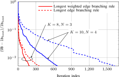
Figure 3: Convergence examples of Algorithm 1 with the longest edge branching rule and longest weighted edge branching rule over two random channel realizations corresponding to the network settings $(K,N)=(8,3)$ and $(K,N)=(10,4)$. The weights are taken as $\mathbf{w}=[0.59;0.31;0.1]$ for $N=3$, and $\mathbf{w}=[0.097;0.519;0.135;0.249]$ for $N=4$.

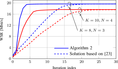
(a) Convergence behavior of the considered schemes

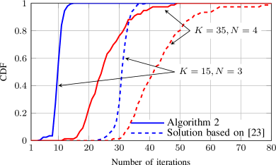
(b) CDF of the number of iteration required to converge.

Figure 4: Convergence speed comparison of Algorithm 2 and the solution modified from the one in [23] with different network settings. The weights are taken as $\mathbf{w}=[0.59;0.31;0.1]$ for $N=3$, and $\mathbf{w}=[0.097;0.519;0.135;0.249]$ for $N=4$.

In Fig. 4, we evaluate the convergence speed of Algorithm 2 compared to the solution modified from the one in [23] with different settings of $(K,N)$. In particular, Fig. 4(a) plots the convergence behavior of the two schemes over two random channels realizations. Fig. 4(b) plots the cumulative distribution function (CDF) of the required number of iterations to converge. The two schemes stop when the increase in the objective value achieved in the last 3 iterations is less than $10^{-2}$. For each channel realization, the same random initial point is used by both schemes for the fairness. We can observe from the figure that the convergence speed of Algorithm 2 is superior in all cases of considered network settings. It is worth mentioning that the two schemes usually, but not always, converge to a same value, and achieve almost the same average performance.

In Fig. 5, we provide an numerical example showing the convergence behavior of the FW solution (see discussion about FW solution in Remark 6 and the detail of the solution in Appendix B) in comparison with the proposed InAp-based solution. For the FW solution, the performance of the diminishing step size rule [50] and the adaptive step size rule [51] are provided. The FW schemes stop when the FW gap is smaller than 1, or the number of iteration exceeds $10^{6}$. All schemes use the same random starting point. We can observe from the figure that, with the two step size rules, the FW solution requires sufficiently large amount of iterations to reach a good performance.

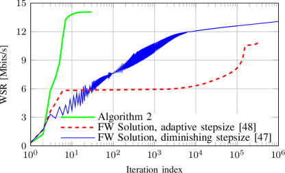
Figure 5: Convergence examples of Algorithm 2 in comparison with FW solution (discussed in Remark 6) with two different step size rules provided in [50] and [51] over a random channel realization corresponding to the network setting $(K,N)=(10,4)$, $\mathbf{w}=[0.097;0.519;0.135;0.249]$.

VI-B Performance Comparison between Optimal Solution and Suboptimal InAp-based Solution.

We now evaluate the performance of Algorithm 2 in terms of WSR using the globally optimal solution (Algorithm 3) as the baseline. Specifically, Fig. 6(a) plots the average WSR performance as the function of the number of small cell BSs. Fig. 6(b) provides the CDF of the ratio of WSR of Algorithm 2 to the optimal solution. We can observe from Fig. 6(a) that the average WSR performance of Algorithm 2 is very close to the optimal one. In Fig. 6(b), we see that Algorithm 2 is not worse than 96% of the optimal solution for all channels. The results demonstrate the efficiency of the proposed efficient solution in terms of achieving the design objective.

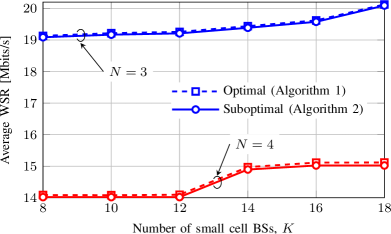
(a) Average WSR

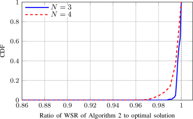
(b) CDF of the ratio of suboptimal solution to optimal solution.

Figure 6: Performance of Algorithm 2 in comparison with optimal solution (Algorithm 1) with different numbers of small cell BSs. The weights are taken as $\mathbf{w}=[0.59;0.31;0.1]$ for $N=3$, and $\mathbf{w}=[0.097;0.519;0.135;0.249]$ for $N=4$.

VI-C Numerical Results of the Distributed Algorithm

In the next set of the experiments, we examine the performance of Algorithm 3. We consider the decentralized architecture network including 5 MEC servers. Each of them serves the BSs lying in a specific area as shown in Fig. 8. Unless otherwise stated, we set the initial values as $q_{id}^{(0)}=y_{id}^{(0)}=1$, for all $i,d$, $\boldsymbol{\xi}^{(0)}=\mathbf{1}$, and $\boldsymbol{\rho}_{d}^{(0)}=\mathbf{1}$ for all $d$.

Fig. 8 shows the function $\textrm{max}(\{||\boldsymbol{\varepsilon}_{d}^{\mathrm{pri}}||_{2}/\bar{\epsilon}_{d}^{\mathrm{pri}}\}_{d},\{||\boldsymbol{\varepsilon}_{d}^{\mathrm{dua}}||_{2}/\bar{\epsilon}_{d}^{\mathrm{dua}}\}_{d})$ over the ADMM iterations in the first InAp iteration of a random channel realization. The function is introduced based on the stopping criterion, which is satisfied when the value of the function is smaller than 1. For the adaptive penalty scheme, we take the relative tolerance $\bar{\epsilon}$ as $10^{-3}$[35]. Other parameters are taken as $\tau=2$, $\beta=5$. The initial values of penalty parameters are set as $m_{d}=m_{0}$ for all $d$; and after 50 iterations, they are fixed as $m_{d}=m_{0}$ for all $d$ [52]. For the fixed penalty parameter scheme, the penalty parameter is set as $m=m_{0}$. Value of $m_{0}$ is specified in the figure. We can observe from the figure that, with the same chosen $m_{0}$, adaptive (penalty) scheme can reach the stopping criteria faster.

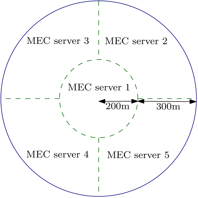
Figure 7: The specified serving areas of the MEC servers considered in the simulations of decentralized networks.

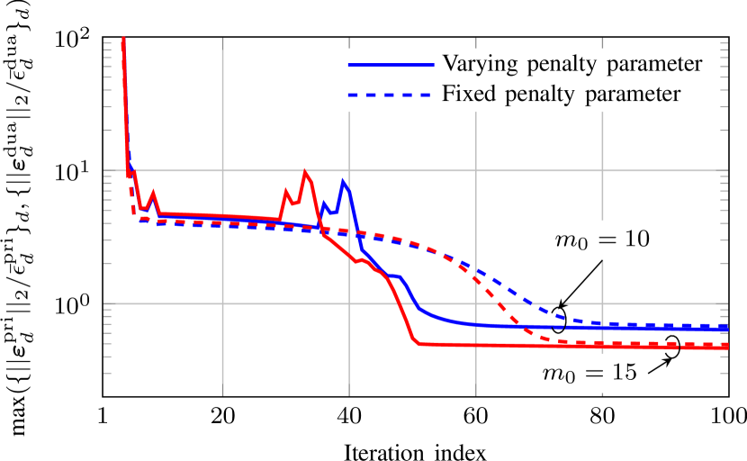
Figure 8: Relative residuals of fixed and varying penalty parameter schemes over ADMM iterations at the first InAp iteration of a random channel realization. The network setting is $(K,N)=(16,5)$. We take $w_{i}=1/N$ for all $i$.

In Fig. 9, we show the achieved WSR of Algorithm 3 compared to the centralized solution (obtained by Algorithm 2 using the solver) over two random channel realizations. Specifically, Fig. 9(a) plots the achieved WSR as a function of the total number of ADMM iterations, while Fig. 9(b) shows the relative gap between the centralized and distributed solutions. To this end, let us denote by $f$ the WSR at an ADMM iteration which is calculated by using the beamforming vectors obtained at the iteration, and denote by $f^{\ast}$ the centralized solution. Then the relative gap is defined as $|f-f^{\ast}|/f^{\ast}$. We take relative tolerance $\bar{\epsilon}$ as $10^{-3}$. In each InAp iteration, the ADMM procedure stops when the termination criterion is met or when the number of ADMM iterations exceeds $I_{\textrm{ADMM}}$. We take $I_{\textrm{ADMM}}$ as 20 and 70. This consideration is to illustrate the heuristic usage of the ADMM discussed in Remark 10. We can observe that the total number of ADMM iterations reduces remarkably with appropriate value of $I_{\textrm{ADMM}}$. We note that the WSR over the ADMM iterations is not necessary to be monotonic because the ADMM works on the augmented Lagrangian function. We also note that when the ADMM procedure converges, the sequence of WSR values corresponding to the outer stage is monotonically increasing as Algorithm 2. However, in this figure, since $I_{\textrm{ADMM}}$ is applied, the sequence can be not monotonic since the parameters of the outer stage are updated even when the ADMM has not converged.

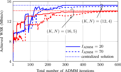
(a) Achieved WSR

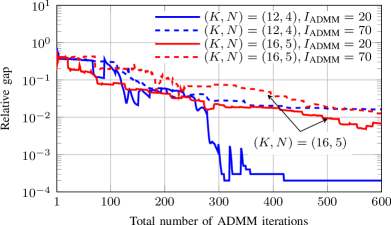
(b) Relative gap, $|f-f^{\ast}|/f^{\ast}$

Figure 9: Achieved WSR of Algorithm 3 compared to centralized solution over two random channel realizations corresponding to network settings $(K,N)=(12,4)$ and $(K,N)=(16,5)$. We take $\mathbf{w}=[0.097;0.519;0.135;0.249]$ for $N=4$, and $w_{i}=1/N$, for all $i$, for $N=5$.

VI-D Performance Comparison between Different CoMP Strategies

In the final set of experiments, we study the WSR performance of the noncoherent JT in comparison with the other CoMP strategies, i.e., coherent JT, and CB. In CB scheme, each of users is only served by the nearest BS. We provide the WSR performance of the noncoherent JT based on Algorithm 2 due to its low complexity and near-optimal performance. We also provide the noncoherent JT using MRT scheme as a benchmark. The solutions of the coherent JT and CB are derived based on that in [44].

Fig. 10 plots the average WSR performance of the considered schemes as functions of the number of small cell BSs. An interesting result observed from the figure is that CB scheme might fail to exploit the densification gain. Another result is that the coherent JT is naturally superior to the others. Therefore, in the networks where the coherent JT is feasible, this scheme should be deployed to achieve maximum spectral efficiency. However, when the synchronization accuracy is not sufficient, the noncoherent JT with the proposed solution is a promising candidate for dense small cell networks, since it outperforms the MRT scheme and CB, and is capable of exploiting densification gain (the performance increases when $K$ increases).

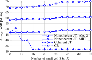
(a) $N=3$

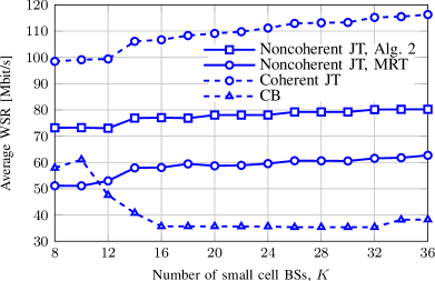
(b) $N=5$

Figure 10: Average WSR performance of the considered noncoherent JT schemes, coherent JT, and CB with different numbers of small cell BSs. The weights are taken as $\mathbf{w}=\boldsymbol{1}$ for all cases of $N$.

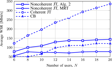
(a) $K=15$

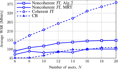
(b) $K=25$

Figure 11: Average WSR performance of the considered noncoherent JT schemes, coherent JT, and CB with different numbers of users. We take $K$ as 15 and 25. The weights are taken as $\mathbf{w}=\boldsymbol{1}$ for all cases of $N$.

In Fig. 11, we show the average WSR performance of the considered schemes as the functions of the number of users $N$ for two cases of $K$. The main result observed from the figure is that the WSR performance of the noncoherent JT with proposed solution, coherent JT and CB increase when $N$ increases. This implies that the three schemes are capable of exploiting the user diversity gain. The results also confirm the observations taken from Fig. 10, i.e., the coherent JT outperforms the others, and the noncoherent JT with the proposed solution outperforms the MRT scheme and CB in all cases of $N$. We can see that, when $N$ is large, the CB outperforms the noncoherent JT with the MRT scheme. This might be because the MRT scheme only considers power allocation, and thus it cannot provide good interference management.

VII Conclusion

We have investigated downlink noncoherent JT in dense small cell networks. Particularly, we have considered the problem of designing beamforming vectors at the macro cell and small cell BSs for maximizing WSR. Because the problem is intractable, we have developed a BRnB algorithm to achieve globally optimal solution. In addition, for practical implementation, we have developed a low-complexity algorithm based on the IA optimization framework, which has been numerically shown to be able to achieve near optimal performance. Moreover, in order to implement the InAp-based solution on decentralized networks using MEC servers, we have provided a distributed algorithm based on the ADMM. The results have revealed that noncoherent JT is capable of exploiting densitification gain and outperforming the CB. It is also feasible to implement the transmission scheme distributively, and it does not require as strict synchronization accuracy as the coherent JT. Thus, noncoherent JT is a promising transmission scheme for dense small cell networks in terms of the WSR performance.

Appendix A Proof of Lemmas

A-A Proof of Lemma 2

The proof is based on that of [21, Theorem 1]. The if part is obvious since $\tilde{\mathcal{S}}_{\mathrm{SD}}(\mathbf{r})$ is the SDR of $\tilde{\mathcal{S}}(\mathbf{r})$ achieved by removing rank-one constraints. Thus we focus on the only-if part, i.e., if $\tilde{\mathcal{S}}_{\mathrm{SD}}(\mathbf{r})$ is nonempty, $\tilde{\mathcal{S}}(\mathbf{r})$ is nonempty. If there exists $\mathbf{V}^{\prime}{}_{ik}\in\tilde{\mathcal{S}}_{\mathrm{SD}}(\mathbf{r})$ such that $\mathrm{rank}(\mathbf{V}_{ik})\leq 1,$$\forall i\in\mathcal{N},\forall k\in\mathcal{K}$, then $\tilde{\mathcal{S}}(\mathbf{r})$ is nonempty which completes the proof. Now suppose that there exists $\mathbf{V}^{\prime}_{uv}\in\tilde{\mathcal{S}}_{\mathrm{SD}}(\mathbf{r})$ where $\mathrm{rank}(\mathbf{V}^{\prime}_{uv})>1$ for some $(u,v)$. Then consider the problem

$$\underset{\mathbf{V}}{\operatorname*{maximize}} \;\mathbf{h}_{uv}\mathbf{V}\mathbf{h}_{uv}^{\mbox{\scriptsize H}}$$ (32a)

$$\operatorname*{subject\leavevmode\nobreak\ to} \;\mathbf{h}_{jv}\mathbf{V}\mathbf{h}_{jv}^{\mbox{\scriptsize H}}\leq\mathbf{h}_{jv}\mathbf{V}^{\prime}_{uv}\mathbf{h}_{jv}^{\mbox{\scriptsize H}},\forall j\neq u$$ (32b)

$$\;\operatorname{tr}(\mathbf{V})\leq\operatorname{tr}(\mathbf{V}^{\prime}_{uv}),\mathbf{V}\in\mathbb{S}_{+}^{M_{v}}.$$ (32c)

It is proved based on a primal-dual analysis that (32) always has a rank-one solution (c.f [55, Appendix III]), which completes the proof.

A-B Proof of Lemma 3

The proof is based on the convergence analysis of BRnB in [30, 46]. Particularly, the reduction is valid, i.e., no feasible point in a box having better performance than $\mathtt{lb}_{\mathrm{best}}$ is lost after the reduction. The bounding guarantees that the upper bound of a box is non-increasing and $\mathtt{lb}_{\mathrm{best}}$ is non-decreasing. Thus the gap $\mathtt{UB}-\mathtt{lb}_{\mathrm{best}}$ is monotonically decreasing. In addition, the bisection partition in the branching is exhaustive [30]. These lead to $(\mathtt{UB}-\mathtt{lb}_{\mathrm{best}})\rightarrow 0$ as $t\rightarrow\infty$, i.e., the gap of the bounds uniformly converges to zero. This completes the proof.

A-C Proof of Lemma 4

To prove the first statement, we show that: (i) the constraints in (13b) hold with equality at optimality, and (ii) vectors $\{\mathbf{v}_{ik}^{\star}\}$ achieve optimal value of (3). For (i), suppose that (13b) is inactive at the optimality for some $i$, then there exists $\mu^{\prime}_{i}>\mu_{i}^{\star}$ such that constraint $i$ in (13b) holds with equality. Thus, the point with $\mu^{\prime}_{i}$ instead of $\mu_{i}^{\star}$ is still feasible and results in a strictly larger objective value, since $\log(1+\mu^{\prime}_{i})>\log(1+\mu_{i}^{\star})$. This contradicts with the assumption that an optimal solution has been achieved.

For (ii), suppose that there exists a feasible point of (3) denoted by $\{\mathbf{v}^{\prime}_{ik}\}$ such that ${\textstyle\sum_{i\in\mathcal{N}}}w_{i}\log(1+\gamma_{i}(\{\mathbf{v}^{\prime}_{ik}\}))>{\textstyle\sum_{i\in\mathcal{N}}}w_{i}\log(1+\mu_{i}^{\star})$, then we determine $\mu^{\prime}_{i}=\gamma_{i}(\{\mathbf{v}^{\prime}_{ik}\})$. Clearly, $(\{\mathbf{v}^{\prime}_{ik}\},\{\mu^{\prime}_{i}\})$ is a feasible point of (13) which achieves larger objective value than $(\{\mathbf{v}_{ik}^{\star}\},\{\mu_{i}^{\star}\})$. Again, this contradicts with the assumption that $(\{\mathbf{v}_{ik}^{\star}\},\{\mu_{i}^{\star}\})$ is optimal.

Similarly, for the converse, we can show by contradiction that there exist no feasible points of (13) which can achieve better objective value than $(\{\mathbf{v}_{ik}^{\ast}\},\{\gamma_{i}(\{\mathbf{v}_{ik}^{\ast}\})\})$. Finally, the the final statement follows the fact (i).

A-D Proof of Lemma 5

By contradiction, we can justify that at optimality all constraints in (17b) hold with equality, leading to $\sqrt{1+\mu_{i}^{(t)}}=1/\pi_{i}^{(t)}$ $\forall\,i,t$. Let us consider iteration $t$. According to the principles of the InAp, the solution to (17) in iteration $t$ is feasible to the problem in iteration $(t+1)$, and thus ${\textstyle\sum_{i\in\mathcal{N}}}\tilde{w}_{i}^{(t)}\pi_{i}^{(t)}\geq{\textstyle\sum_{i\in\mathcal{N}}}\tilde{w}_{i}^{(t)}\pi_{i}^{(t+1)}$ which is equivalent to

$${\textstyle\sum_{i\in\mathcal{N}}}w_{i}\sqrt{(1+\mu_{i}^{(t)})/(1+\mu_{i}^{(t)})} \geq{\textstyle\sum_{i\in\mathcal{N}}}w_{i}\sqrt{(1+\mu_{i}^{(t)})/(1+\mu_{i}^{(t+1)})}$$

$$\Leftrightarrow{\textstyle\sum_{i\in\mathcal{N}}}\underset{=\log(1+\mu_{i}^{(t)})}{w_{i}\underbrace{(J^{(t)}-2\sqrt{(1+\mu_{i}^{(t)})/(1+\mu_{i}^{(t)})})}} \leq{\textstyle\sum_{i\in\mathcal{N}}}w_{i}\underset{\leq\log(1+\mu_{i}^{(t+1)})}{\underbrace{(J^{(t)}-2\sqrt{(1+\mu_{i}^{(t)})/(1+\mu_{i}^{(t+1)})})}}$$

where $J^{(t)}=\log(1+\mu_{i}^{(t)})+2$. In addition, problem (13) is upper bounded by a finite value due to power constraints (13c). This completes the proof.

A-E Proof of Lemma 8

The proof is based on the convergence analysis of ADMM in [35]. Firstly, we note that the feasible set of (17) is convex and nonempty for all InAp iterations, and so is that of (19). The objective of (17) is bounded. Consequently, sets $\tilde{\mathcal{S}}$ and $\hat{\mathcal{S}}_{d}$ are nonempty, and the problems (24), (25), and (26) are solvable [35, Assumption 1]. Secondly, we recall that the considered problem is only constrained by the maximum transmit power at the BSs. Thus, problem (19) is strictly feasible. Consequently, the assumption that the unaugmented Lagrangian (i.e., function (23) with $m=0$) has a saddle point holds [35, Assumption 2]. With these, the lemma follows the statement in [35, Section 3.2.1].

Appendix B A First-Order Algorithm Solving (3) via Conditional Gradient Method

In this appendix, we present a first-order solution for solving (3) using Frank-Wolfe’s method. To proceed, let us define some notations as $\mathbf{H}_{ik}=\mathbf{h}_{ik}^{\mbox{\scriptsize H}}\mathbf{h}_{ik}$, $\hat{\mathbf{H}}_{ik}=\textrm{blkdiag}\{\underset{N}{\underbrace{\mathbf{H}_{ik},...,\mathbf{H}_{ik}}}\}$, $\mathbf{H}_{i}=\textrm{blkdiag}\{\hat{\mathbf{H}}_{i1},...,\hat{\mathbf{H}}_{i(k+1)}\}$, $\mathbf{v}_{k}=[\mathbf{v}_{1k};...;\mathbf{v}_{Nk}]$, $\mathbf{v}=[\mathbf{v}_{1};...;\mathbf{v}_{k+1}]$, $\hat{\mathbf{G}}_{ik}=\textrm{blkdiag}\{\underset{i-1}{\underbrace{\mathbf{H}_{ik},...,\mathbf{H}_{ik}}},\linebreak\boldsymbol{0},\underset{N-i}{\underbrace{\mathbf{H}_{ik},...,\mathbf{H}_{ik}}}\}$, and $\mathbf{G}_{i}=\textrm{blkdiag}\{\hat{\mathbf{G}}_{i1},...,\hat{\mathbf{G}}_{i(k+1)}\}$. Then we rewrite the objective function as

$$g(\mathbf{v})={\textstyle\sum_{i\in\mathcal{N}}}w_{i}\log\Bigl{(}\frac{\mathbf{v}^{\mbox{\scriptsize H}}\mathbf{H}_{i}\mathbf{v}+\sigma_{i}^{2}}{\mathbf{v}^{\mbox{\scriptsize H}}\mathbf{G}_{i}\mathbf{v}+\sigma_{i}^{2}}\Bigr{)}$$

For ease of exposition, we convert $g(\mathbf{v})$ in the real-domain as

$$g(\tilde{\mathbf{v}})={\textstyle\sum_{i\in\mathcal{N}}}w_{i}\log\Bigl{(}\frac{\tilde{\mathbf{v}}^{\mbox{\scriptsize T}}\bar{\mathbf{H}}_{i}\tilde{\mathbf{v}}+\sigma_{i}^{2}}{\tilde{\mathbf{v}}^{\mbox{\scriptsize T}}\bar{\mathbf{G}}_{i}\tilde{\mathbf{v}}+\sigma_{i}^{2}}\Bigr{)}$$

where $\tilde{\mathbf{v}}=[\mathrm{Re}\{\mathbf{v}\};\mathrm{Im}\{\mathbf{v}\}]$, $\bar{\mathbf{H}}_{i}=[\mathrm{Re}\{\mathbf{H}_{i}\},-\mathrm{Im}\{\mathbf{H}_{i}\};\mathrm{Im}\{\mathbf{H}_{i}\},\mathrm{Re}\{\mathbf{H}_{i}\}]$, and $\bar{\mathbf{G}}_{i}=[\mathrm{Re}\{\mathbf{G}_{i}\},\linebreak-\mathrm{Im}\{\mathbf{G}_{i}\};\mathrm{Im}\{\mathbf{G}_{i}\},\mathrm{Re}\{\mathbf{G}_{i}\}]$. Let $\tilde{\mathbf{v}}^{(t)}$ be a feasible point, then the gradient of $g(\tilde{\mathbf{v}})$ at $\tilde{\mathbf{v}}^{(t)}$ is

$$\nabla_{\tilde{\mathbf{v}}}g(\tilde{\mathbf{v}}^{(t)}) = {\textstyle\sum_{i\in\mathcal{N}}}w_{i}\Bigl{(}\frac{2\bar{\mathbf{H}}_{i}\tilde{\mathbf{v}}^{(t)}}{(\tilde{\mathbf{v}}^{(t)})^{\mbox{\scriptsize T}}\bar{\mathbf{H}}_{i}\tilde{\mathbf{v}}^{(t)}+\sigma_{i}^{2}}-\frac{2\bar{\mathbf{G}}_{i}\tilde{\mathbf{v}}^{(t)}}{(\tilde{\mathbf{v}}^{(t)})^{\mbox{\scriptsize T}}\bar{\mathbf{G}}_{i}\tilde{\mathbf{v}}^{(t)}+\sigma_{i}^{2}}\Bigr{)}.$$ (33)

Then the linear optimization oracle at each iteration is

$$\tilde{\mathbf{v}}^{\ast}=\textrm{argmax}(\nabla g(\tilde{\mathbf{v}}^{(t)})^{\mbox{\scriptsize T}}\tilde{\mathbf{v}}|\tilde{\mathbf{v}}_{k}^{\mbox{\scriptsize T}}\tilde{\mathbf{v}}_{k}\leq P_{k},\forall k\in\mathcal{K})$$ (34)

where $\tilde{\mathbf{v}}_{k}=[\mathrm{Re}\{\mathbf{v}_{k}\};\mathrm{Im}\{\mathbf{v}_{k}\}]$. As the objective and the feasible set of the above problem are separable with respect to $\tilde{\mathbf{v}}_{k}$, it is easy to see that (34) has the following closed-form expression

$$\tilde{\mathbf{v}}_{k}^{\ast}=\sqrt{P_{k}/(\mathbf{c}_{k}^{\mbox{\scriptsize T}}\mathbf{c}_{k})}\mathbf{c}_{k}$$ (35)

where $\mathbf{c}_{k}=\{\nabla g(\tilde{\mathbf{v}}^{(t)})\}_{\tilde{\mathbf{v}}_{k}}$ is the vector including the elements of $\nabla g(\tilde{\mathbf{v}}^{(t)})$ associated with $\tilde{\mathbf{v}}_{k}$.

The first-order iterative algorithm for solving (3) is outlined as follows:

Initialization: Set small $\epsilon_{\mathrm{G}}$, $t\coloneqq 1$, choose initial point $\tilde{\mathbf{v}}^{(1)}$.

repeat

Generate $\nabla g(\tilde{\mathbf{v}}^{(t)})$, then determine $\tilde{\mathbf{v}}^{\ast}$ according to (35).

if $\nabla g(\tilde{\mathbf{v}}^{(t)})^{\mbox{\scriptsize T}}(\tilde{\mathbf{v}}^{\ast}-\tilde{\mathbf{v}}^{(t)})\leq\epsilon_{\mathrm{G}}$

Stop and return $\tilde{\mathbf{v}}^{(t)}$

else

Choose step size $\alpha^{(t)}\in[0,1]$, then update $\tilde{\mathbf{v}}^{(t+1)}:=(1-\alpha^{(t)})\tilde{\mathbf{v}}^{(t)}+\alpha^{(t)}\tilde{\mathbf{v}}^{\ast}$

$t:=t+1$.

end

In each iteration, the new iterate $\tilde{\mathbf{v}}^{(t+1)}$ is determined by moving the current iterate $\tilde{\mathbf{v}}^{(t)}$ along the dictated direction $\tilde{\mathbf{v}}^{\ast}-\tilde{\mathbf{v}}^{(t)}$ with step size $\alpha^{(t)}\in(0,1]$.

Smoothness of $g(\mathbf{v})$

We now investigate the smoothness of $g(\tilde{\mathbf{v}})$, which is essential for the convergence result of the Frank-Wolfe (FW) based method above to be provided in the next subsection. In particular, the Hessian of $g(\mathbf{v})$ at $\tilde{\mathbf{v}}^{(t)}$ is given by

$$\nabla_{\tilde{\mathbf{v}}}^{2}g(\tilde{\mathbf{v}}^{(t)})={\textstyle\sum_{i\in\mathcal{N}}}w_{i}\Bigl{(}\frac{2\bar{\mathbf{H}}_{i}}{(\tilde{\mathbf{v}}^{(t)})^{\mbox{\scriptsize T}}\bar{\mathbf{H}}_{i}\tilde{\mathbf{v}}^{(t)}+\sigma_{i}^{2}}-\frac{4\bar{\mathbf{H}}_{i}\tilde{\mathbf{v}}^{(t)}(\tilde{\mathbf{v}}^{(t)})^{\mbox{\scriptsize T}}\bar{\mathbf{H}}_{i}^{\mbox{\scriptsize T}}}{((\tilde{\mathbf{v}}^{(t)})^{\mbox{\scriptsize T}}\bar{\mathbf{H}}_{i}\tilde{\mathbf{v}}^{(t)}+\sigma_{i}^{2})^{2}}\\ -\frac{2\bar{\mathbf{G}}_{i}}{(\tilde{\mathbf{v}}^{(t)})^{\mbox{\scriptsize T}}\bar{\mathbf{G}}_{i}\tilde{\mathbf{v}}^{(t)}+\sigma_{i}^{2}}+\frac{4\bar{\mathbf{G}}_{i}\tilde{\mathbf{v}}^{(t)}(\tilde{\mathbf{v}}^{(t)})^{\mbox{\scriptsize T}}\bar{\mathbf{G}}_{i}^{\mbox{\scriptsize T}}}{((\tilde{\mathbf{v}}^{(t)})^{\mbox{\scriptsize T}}\bar{\mathbf{G}}_{i}\tilde{\mathbf{v}}^{(t)}+\sigma_{i}^{2})^{2}}\Bigr{)}.$$ (36)

It is trivial to show that $||\nabla_{\tilde{\mathbf{v}}}^{2}g(\tilde{\mathbf{v}}^{(t)})||_{2}\leq{\displaystyle\rho_{\mathrm{L}}\triangleq}\sum_{i\in\mathcal{N}}w_{i}(\frac{2}{\sigma_{i}^{2}}||\bar{\mathbf{H}}_{i}||_{2}+\frac{4P_{\mathrm{total}}}{\sigma_{i}^{4}}||\bar{\mathbf{H}}_{i}||_{2}^{2}+\frac{2}{\sigma_{i}^{2}}||\bar{\mathbf{G}}_{i}||_{2}+\frac{4P_{\mathrm{total}}}{\sigma_{i}^{4}}||\bar{\mathbf{G}}_{i}||_{2}^{2})$, where $P_{\mathrm{total}}=\sum_{k}P_{k}$, which means $g(\tilde{\mathbf{v}})$ is a $\rho_{\mathrm{L}}$-smooth function [56].

Step Size Rules and Convergence

Note that the FW-type method for nonconvex problems is not monotonically increasing, and thus a proper choice of the step size $\alpha^{(t)}$ at each iteration is critical for the convergence. This issue is relatively open and receiving increasing interest but there are some known step size rules for the conditional gradient method. One is the line-search rule: $\alpha^{(t)}=\textrm{argmax}(g((1-\alpha)\tilde{\mathbf{v}}^{(t)}+\tilde{\mathbf{v}}^{\ast})|\alpha^{(t)}\in[0,1])$ [49], but it is not cost effective here since the one-dimentional search does not admit a closed-form solution. An adaptive step size rule is recently proposed in [51]. The diminishing step size rule $\alpha^{(t)}=t^{-\omega}$, where $\omega\in(0.5,1]$, can also be used [50].

For the convergence, we recall that the feasible set of problem (3) is convex and compact. In addition, we have shown that $g(\tilde{\mathbf{v}})$ has a finite Lipschitz gradient constant $\rho_{\mathrm{L}}$. Thus, by the mentioned step size rules, it is guaranteed that the iterative procedure converges to a stationary point of (3) [49, 50, 51]. In addition, for the line-search and adaptive step size rules, it is proved that the convergence rate is $\mathcal{O}(1/\sqrt{t})$ [49, Theorem 1], [51, Theorem 1].

References

• [1] Q.-D. Vu, L.-N. Tran, and M. Juntti, “Distributed noncoherent transmit beamforming for dense small cell networks,” in Proc. IEEE ICASSP 2019, May 2019.
• [2] Ericsson, “Mobility report,” Nov. 2018.
• [3] 3GPP, “Study on scenarios and requirements for next generation access technologies,” TR 38.913, 2017.
• [4] X. Ge, S. Tu, G. Mao, C. Wang, and T. Han, “5G ultra-dense cellular networks,” IEEE Wireless Commun. Mag., vol. 23, no. 1, pp. 72–79, Feb. 2016.
• [5] J. Hoydis, M. Kobayashi, and M. Debbah, “Green small-cell networks,” IEEE Vehicular Technology Magazine, vol. 6, no. 1, pp. 37–43, March 2011.
• [6] Small Cell Forum, “Small cell siting challenges,” Feb. 2017.
• [7] P. Rost, C. J. Bernardos, A. D. Domenico, M. D. Girolamo, M. Lalam, A. Maeder, D. Sabella, and D. Wübben, “Cloud technologies for flexible 5G radio access networks,” IEEE Commun. Mag., vol. 52, no. 5, pp. 68–76, May 2014.
• [8] Ericsson, “Cloud RAN-the benefits of virtualization, centralization and coordination,” Sep. 2015.
• [9] M. Peng, C. Wang, V. Lau, and H. V. Poor, “Fronthaul-constrained cloud radio access networks: insights and challenges,” IEEE Wireless Commun. Mag., vol. 22, no. 2, pp. 152–160, April 2015.
• [10] S. C. Forum, “Edge computing made simple,” Dec. 2017.
• [11] ETSI, “Cloud RAN and MEC: A perfect pairing,” The European Telecommunications Standards Institute, White paper, Feb. 2018.
• [12] T. X. Tran, A. Hajisami, P. Pandey, and D. Pompili, “Collaborative mobile edge computing in 5G networks: New paradigms, scenarios, and challenges,” IEEE Commun. Mag., vol. 55, no. 4, pp. 54–61, April 2017.
• [13] P. Mach and Z. Becvar, “Mobile edge computing: A survey on architecture and computation offloading,” IEEE Communications Surveys Tutorials, vol. 19, no. 3, pp. 1628–1656, thirdquarter 2017.
• [14] Ericsson, “Distributed cloud infrastructure,” 2017.
• [15] ETSI, “Mobile edge computing - a key technology towards 5G,” The European Telecommunications Standards Institute, White paper, Sep. 2015.
• [16] J. Zheng, Y. Wu, N. Zhang, H. Zhou, Y. Cai, and X. Shen, “Optimal power control in ultra-dense small cell networks: A game-theoretic approach,” IEEE Trans. Wireless Commun., vol. 16, no. 7, pp. 4139–4150, July 2017.
• [17] D. Lee, H. Seo, B. Clerckx, E. Hardouin, D. Mazzarese, S. Nagata, and K. Sayana, “Coordinated multipoint transmission and reception in LTE-advanced: deployment scenarios and operational challenges,” IEEE Commun. Mag., vol. 50, no. 2, pp. 148–155, Feb. 2012.
• [18] D. Gesbert, S. Hanly, H. Huang, S. Shamai Shitz, O. Simeone, and W. Yu, “Multi-cell MIMO cooperative networks: A new look at interference,” IEEE J. Sel. Areas Commun., vol. 28, no. 9, pp. 1380–1408, Dec 2010.
• [19] A. Checko, H. L. Christiansen, Y. Yan, L. Scolari, G. Kardaras, M. S. Berger, and L. Dittmann, “Cloud RAN for Mobile Networks–A Technology Overview,” IEEE Commun. Surveys Tuts., vol. 17, no. 1, pp. 405–426, Firstquarter 2015.
• [20] G. C. Alexandropoulos, P. Ferrand, J. Gorce, and C. B. Papadias, “Advanced coordinated beamforming for the downlink of future LTE cellular networks,” IEEE Commun. Mag., vol. 54, no. 7, pp. 54–60, July 2016.
• [21] E. Björnson, M. Kountouris, and M. Debbah, “Massive MIMO and small cells: Improving energy efficiency by optimal soft-cell coordination,” in 20th International Conference on Telecommunications (ICT), May 2013, pp. 1–5.
• [22] J. Li, E. Björnson, T. Svensson, T. Eriksson, and M. Debbah, “Joint precoding and load balancing optimization for energy-efficient heterogeneous networks,” IEEE Trans. Wireless Commun., vol. 14, no. 10, pp. 5810–5822, Oct 2015.
• [23] C. Pan, H. Ren, M. Elkashlan, A. Nallanathan, and L. Hanzo, “The non-coherent ultra-dense C-RAN is capable of outperforming its coherent counterpart at a limited fronthaul capacity,” IEEE J. Sel. Areas Commun., vol. 36, no. 11, pp. 2549–2560, Nov. 2018.
• [24] T. V. Chien, E. Björnson, and E. G. Larsson, “Joint power allocation and user association optimization for massive MIMO systems,” IEEE Trans. Wireless Commun., vol. 15, no. 9, pp. 6384–6399, Sept 2016.
• [25] J. Proakis, Digital Communications, 4th ed., J. Proakis, Ed.   McGraw-Hill, 2001.
• [26] Lizhong Zheng and D. N. C. Tse, “Communication on the Grassmann manifold: a geometric approach to the noncoherent multiple-antenna channel,” IEEE Trans. Inf. Theory, vol. 48, no. 2, pp. 359–383, Feb. 2002.
• [27] A. Lapidoth and S. M. Moser, “Capacity bounds via duality with applications to multiple-antenna systems on flat-fading channels,” IEEE Trans. Inf. Theory, vol. 49, no. 10, pp. 2426–2467, Oct 2003.
• [28] M. Kobayashi and G. Caire, “An iterative water-filling algorithm for maximum weighted sum-rate of Gaussian MIMO-BC,” IEEE J. Sel. Areas Commun., vol. 24, no. 8, pp. 1640–1646, Aug 2006.
• [29] Z.-Q. Luo and S. Zhang, “Dynamic spectrum management: Complexity and duality,” vol. 2, no. 1, pp. 57–73, Feb 2008.
• [30] H. Tuy, F. Al-Khayyal, and P. T. Thach, “Monotonic optimization: Branch and cut methods,” in Essays and Surveys in Global Optimization.   Springer, 2005, pp. 39–78.
• [31] B. R. Marks and G. P. Wright, “A general inner approximation algorithm for nonconvex mathematical programs,” Operations Research, vol. 26, no. 4, pp. 681–683, August 1978.
• [32] A. Beck, A. Ben-Tal, and L. Tetruashvili, “A sequential parametric convex approximation method with applications to nonconvex truss topology design problems,” Journal of Global Optimization, vol. 47, no. 1, pp. 29–51, 2010.
• [33] K.-G. Nguyen, Q.-D. Vu, M. Juntti, and L.-N. Tran, “Distributed solutions for energy efficiency fairness in multicell MISO downlink,” IEEE Trans. Wireless Commun., vol. 16, no. 9, pp. 6232–6247, Sept 2017.
• [34] Q.-D. Vu, L.-N. Tran, M. Juntti, and E.-K. Hong, “Energy-efficient bandwidth and power allocation for multi-homing networks,” IEEE Trans. Signal Process., vol. 63, no. 7, pp. 1684–1699, April 2015.
• [35] S. Boyd, N. Parikh, E. Chu, B. Peleato, and J. Eckstein, “Distributed optimization and statistical learning via the alternating direction method of multipliers,” Foundations and Trends in Machine Learning, vol. 3, no. 1, pp. 1–122, 2011.
• [36] C. Shen, T. Chang, K. Wang, Z. Qiu, and C. Chi, “Distributed robust multicell coordinated beamforming with imperfect CSI: An ADMM approach,” IEEE Trans. Signal Process., vol. 60, no. 6, pp. 2988–3003, June 2012.
• [37] Z. Xu, C. Yang, G. Li, Y. Liu, and S. Xu, “Energy-efficient CoMP precoding in heterogeneous networks,” IEEE Trans. Signal Process., vol. 62, no. 4, pp. 1005–1017, Feb 2014.
• [38] Q.-D. Vu, L.-N. Tran, R. Farrell, and E.-K. Hong, “Energy-efficient zero-forcing precoding design for small-cell networks,” IEEE Trans. Commun., vol. 64, no. 2, pp. 790–804, Feb 2016.
• [39] T. X. Tran and D. Pompili, “Dynamic radio cooperation for user-centric Cloud-RAN with computing resource sharing,” IEEE Trans. Wireless Commun., vol. 16, no. 4, pp. 2379–2393, April 2017.
• [40] T. T. Vu, D. T. Ngo, M. N. Dao, S. Durrani, D. H. N. Nguyen, and R. H. Middleton, “Energy efficiency maximization for downlink cloud radio access networks with data sharing and data compression,” IEEE Trans. Wireless Commun., vol. 17, no. 8, pp. 4955–4970, Aug 2018.
• [41] F. Zhuang and V. K. N. Lau, “Backhaul limited asymmetric cooperation for MIMO cellular networks via semidefinite relaxation,” IEEE Trans. Signal Process., vol. 62, no. 3, pp. 684–693, Feb 2014.
• [42] P. Luong, F. Gagnon, C. Despins, and L. Tran, “Optimal joint remote radio head selection and beamforming design for limited fronthaul C-RAN,” IEEE Trans. Signal Process., vol. 65, no. 21, pp. 5605–5620, Nov 2017.
• [43] Q. Shi, M. Razaviyayn, Z. Luo, and C. He, “An iteratively weighted MMSE approach to distributed sum-utility maximization for a MIMO interfering broadcast channel,” IEEE Trans. Signal Process., vol. 59, no. 9, pp. 4331–4340, Sep. 2011.
• [44] L.-N. Tran, M. Hanif, A. Tolli, and M. Juntti, “Fast converging algorithm for weighted sum rate maximization in multicell MISO downlink,” IEEE Signal Process. Lett., vol. 19, no. 12, pp. 872–875, Dec 2012.
• [45] O. Tervo, L.-N. Tran, and M. Juntti, “Optimal energy-efficient transmit beamforming for multi-user MISO downlink,” IEEE Trans. Signal Process., vol. 63, no. 20, pp. 5574–5588, Oct. 2015.
• [46] E. Björnson, G. Zheng, M. Bengtsson, and B. Ottersten, “Robust monotonic optimization framework for multicell MISO systems,” IEEE Trans. Signal Process., vol. 60, no. 5, pp. 2508–2523, May 2012.
• [47] M. Lobo, L. Vandenberghe, S. Boyd, and H. Lebret, “Applications of second-order cone programming,” Linear Algebra Appl., Special Issue on Linear Algebra in Control, Signals and Image Processing, pp. 193–228, Nov. 1998.
• [48] K.-G. Nguyen, Q.-D. Vu, L.-N. Tran, and M. Juntti, “Energy efficiency fairness for multi-pair wireless-powered relaying systems,” IEEE J. Sel. Areas Commun., vol. 37, no. 2, pp. 357–373, Feb. 2019.
• [49] S. Lacoste-Julien, “Convergence rate of frank-wolfe for non-convex objectives,” ArXiv e-prints, Jul 2016.
• [50] H. Wai, J. Lafond, A. Scaglione, and E. Moulines, “Decentralized Frank-Wolfe algorithm for convex and nonconvex problems,” IEEE Transactions on Automatic Control, vol. 62, no. 11, pp. 5522–5537, Nov 2017.
• [51] F. Pedregosa, A. Askari, G. Negiar, and M. Jaggi, “Step-size adaptivity in projection-free optimization,” ArXiv e-prints, Oct. 2018.
• [52] C. Song, S. Yoon, and V. Pavlovic, “Fast ADMM algorithm for distributed optimization with adaptive penalty,” in Proc. 30th AAAI Conf. Artificial Intellidence (AAAI-16), Feb. 2016.
• [53] I. MOSEK ApS, 2014, [Online]. Available: www.mosek.com.
• [54] J. Löfberg, “YALMIP : A toolbox for modeling and optimization in MATLAB,” in Proc. the CACSD Conference, Taipei, Taiwan., 2004. [Online]. Available: http://users.isy.liu.se/johanl/yalmip
• [55] A. Wiesel, Y. C. Eldar, and S. Shamai, “Zero-forcing precoding and generalized inverses,” IEEE Trans. Signal Process., vol. 56, no. 9, pp. 4409–4418, Sept 2008.
• [56] J. Fessler, “Gradient-based methods,” https://web.eecs.umich.edu/ fessler/course/598/l/, 2019.