Optimal Learning with Excitatory and Inhibitory synapses

Abstract

Characterizing the relation between weight structure and input/output statistics is fundamental for understanding the computational capabilities of neural circuits. In this work, I study the problem of storing associations between analog signals in the presence of correlations, using methods from statistical mechanics. I characterize the typical learning performance in terms of the power spectrum of random input and output processes. I show that optimal synaptic weight configurations reach a capacity of 0.5 for any fraction of excitatory to inhibitory weights and have a peculiar synaptic distribution with a finite fraction of silent synapses. I further provide a link between typical learning performance and principal components analysis in single cases. These results may shed light on the synaptic profile of brain circuits, such as cerebellar structures, that are thought to engage in processing time-dependent signals and performing on-line prediction.

Introduction

At the most basic level, neuronal circuits are characterized by the subdivision into excitatory and inhibitory populations, a principle called Dale’s law. Even though the precise functional role of Dale’s law has not yet been understood, the importance of synaptic sign constraints is pivotal in constructing biologically plausible models of synaptic plasticity in the brain Song_training ; NicolaClopathSupervised ; Ingrosso_training ; kimlearning ; Deneve_spikebyspike . The properties of synaptic couplings strongly impact the dynamics and response of neural circuits, thus playing a crucial role in shaping their computational capabilities. It has been argued that the statistics of synaptic weights in neural circuits could reflect a principle of optimality for information storage, both at the level of single-neuron weight distributions Brunel_optimal ; Barbour_whatcanwelearn and inter-cell synaptic correlations Brunel_cortical (e.g. the overabundance of reciprocal connections). A number of theoretical studies, stemming from the pioneering Gardner approach Gardner_spaceofinteractions , have investigated the computational capabilities of stylized classification and memorization tasks in both binary Clopath_storage ; Chapeton_efficient ; Zhang_associative ; RubinBalanced and analog perceptrons Seung_learning ; Clopath_optimal , using synthetic data. With some exceptions mentioned in the following, these studies considered random uncorrelated inputs and outputs, a usual approach in statistical learning theory. One interesting theoretical prediction is that non-negativity constraints imply that a finite fraction of synaptic weights are set to zero at critical capacity Gutfreund_capacity ; Brunel_optimal ; Clopath_optimal , a feature which is consistent with experimental synaptic weight distributions observed in some brain areas, e.g. input fibers to Purkinje cells in the cerebellum.

The need to understand how the interaction between excitatory and inhibitory synapses meditates plasticity and dynamic homeostasis Isaacson_inhibition ; Field_HeterosynapticPlasticity calls for the study of heterogeneous multi-population feed-forward and recurrent models. A plethora of mechanisms for excitatory-inhibitory (E-I) balance of input currents onto a neuron have been proposed Hennequin_review ; ahmadian_dynamical . At the computational level, it has recently been shown that a peculiar scaling of excitation and inhibition with network size, originally introduced to account for the high variability of neural firing activity VanVreeswijkChaosScience ; VanVreeswijkChaoticBalancedStateNeuralComputation ; RenartAsynchronous ; KadmonSompolinsky ; HarishHanselAsynchronous ; BrunelDynamicsSparsely ; TsodyksStateSwitching , carries the computational advantage of noise robustness and stability of memory states in associative memory networks RubinBalanced .

Analyzing training and generalization performance in feed-forward and recurrent networks as a function of statistical and geometrical structure of a task remains an open problem both in computational neuroscience and statistical learning theory goldt_modelling ; Chung_perceptualmanifold ; Cohen_Separability . This calls for statistical models of the low-dimensional structure of data that are at the same time expressive and amenable to mathematical analyses. A few classical studies investigated the effect of “semantic” (among input patterns) and spatial (among neural units) correlations in random classification and memory retrieval Monasson_properties ; Tarkowski_optimal ; Monasson_correlatedpatterns . The latter are important in the construction of associative memory networks for place cell formation in the hippocampal complex Battista_capacity .

For reason of mathematical tractability, the vast majority of analytical studies in binary and analog perceptron models focused on the case where both inputs and outputs are independent and identically distributed. In this work, I relax this assumption and study optimal learning of input/output associations with real-world statistics with a linear perceptron having heterogeneous synaptic weights. I introduce a mean-field theory of an analog perceptron in the presence of weight regularization with sign-constraints, considering two different statistical models for input and output correlations. I derive its critical capacity in a random association task and study the statistical properties of the optimal synaptic weight vector across a diverse range of parameters.

This work is organized as follows. In the first section, I introduce the framework and provide the general definitions for the problem. I first consider a model of temporal (or, equivalently, “semantic”) correlations across inputs and output patterns, assuming statistical independence across neurons. I show that optimal solutions are insensitive to the fraction of E and I weights, as long as the external bias is learned. I derive the weight distribution and show that it is characterized by a finite fraction of zero weights also in the general case of E-I constraints and correlated signals. The assumption of independence is subsequently relaxed and I build on self-averaging adaptive TAP formalism to provide a theory that depends on the spectrum of the sample covariance matrix and the dimensionality of the output signal along the principal components of the input. The implications of these results are discussed in the final section.

Results

Mean-field theory with correlations

Consider the problem of linearly mapping a set of time-correlated signals $x_{i\mu}$, with $i\in 1,...,N$ and $\mu=1,...,M$ from $N_{E}=f_{E}N$ excitatory (E) and $N_{I}=\left(1-f_{E}\right)N$ inhibitory (I) neurons, onto an output signal $y_{\mu}$ using a synaptic vector $\boldsymbol{w}$, in the presence of a learnable constant bias current $b$ (Fig 1).

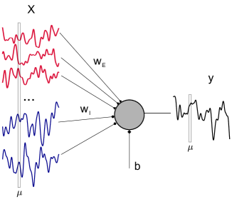
Figure 1: Schematic of the learning problem. A linear perceptron receives $N$ correlated signals (input rates of pre-synaptic neurons) $x_{i\mu}$ and maps them to the output $y_{\mu}$ through $N_{E}=f_{E}N$ excitatory and $N_{I}=\left(1-f_{E}\right)N$ plastic inhibitory weights $w_{i}$, plus an additional bias current $b$.

To account for different statistical properties of E and I input rates, we write the elements of the input matrix as $\left(X\right)_{i\mu}\equiv x_{i\mu}=\bar{x}_{i}+\sigma_{i}\xi_{i\mu}$ with $\bar{x}_{i}=\bar{x}_{E}$ for $i\leq f_{E}N$ and $\bar{x}_{i}=\bar{x}_{I}$ for $i>f_{E}N$ and the same for $\sigma_{i}$. At this stage, the quantities $\xi_{i\mu}$ have unit variance and are uncorrelated across neurons: $\left\langle\xi_{i\mu}\xi_{i\nu}\right\rangle=\delta_{ij}C_{\mu\nu}$. The output signal has average $\left\langle y_{\mu}\right\rangle=\bar{y}$ and variance $\left\langle\left(y_{\mu}-\bar{y}\right)^{2}\right\rangle=\sigma_{y}^{2}$. We initially consider output signals $y_{\mu}$ with the same temporal correlations as the input, namely $\left\langle\delta y_{\mu}\delta y_{\nu}\right\rangle=C_{\mu\nu}$, where $y_{\mu}=\bar{y}+\sigma_{y}\delta y_{\mu}$. For a given input-output set, we are faced with the problem of minimizing the following regression loss (energy) function:

$$E\left(\boldsymbol{w};\gamma,x,y\right)=\frac{1}{2}\sum_{\mu=1}^{M}\left(\sum_{i=1}^{N}w_{i}x_{i\mu}+b-y_{\mu}\right)^{2}+\frac{N\gamma}{2}\sum_{i=1}^{N}w_{i}^{2}$$ (1)

with $w_{i}>0$ for $i\leq f_{E}N$, $w_{i}<0$ otherwise. The typical vector $\boldsymbol{w}$ that solves this sign-constrained least square problem has a squared norm $\sum_{i=1}^{N}w_{i}^{2}=\mathcal{O}\left(1\right)$, hence the scaling of the regularization term $N\gamma$. In order to consider a well defined $N\to\infty$ limit for $E$ and the spectrum of the matrix $C$, we take $M=\alpha N$, with $\alpha$ called the load, as is costumary in mean-field analysis of perceptron problems Gardner_spaceofinteractions . Numerical experiments show that the optimal bias current is of order $\sqrt{N}$, as can be derived in the special case of i.i.d input/output and non-negative synaptic weights $w_{i}$ Clopath_optimal . Optimizing with respect to the bias $b=I\sqrt{N}$ naturally yields solutions $\boldsymbol{w}$ for which

$$N_{E}\bar{w}_{E}\bar{x}_{E}+N_{I}\bar{w}_{I}\bar{x}_{I}+b=\bar{y}$$ (2)

where we call $\bar{w}_{c}=\frac{1}{N_{c}}\sum_{i\in c}w_{i}=\mathcal{O}\left(1/\sqrt{N}\right)$ the average excitatory and inhibitory weight, with $c\in\left\{E,I\right\}$. We call this property balance, in that the same scaling is used in balanced state theory of neural circuits VanVreeswijkChaosScience ; VanVreeswijkChaoticBalancedStateNeuralComputation ; KadmonSompolinsky .

In order to derive a mean-field description for the typical properties of the learned synaptic vector $\boldsymbol{w}$, we employ a statistical mechanics framework in which the minimizer of $E$ is evaluated after averaging across all possible realizations of the input matrix $X$ and output $y$. To do so, we compute the free energy density

$$f=-\frac{1}{\beta N}\left<\log\int{d\mu\left(\boldsymbol{w}\right)}e^{-\beta E}\right>_{x,y}$$ (3)

where $d\mu\left(\boldsymbol{w}\right)$ is the measure implementing the sign-constraints over the synapic weight vector $\boldsymbol{w}$. The brackets in Eq (3) stand for the quenched average over all the quantities $x_{i\mu}$ and $y_{\mu}$, and the inverse temperature $\beta$ will allow us to select weight configurations $\boldsymbol{w}$ which minimize the energy $E$. The free energy $f$ acts as a generating function from which all the statistical quantities of interest can be calculated by appropriate differentiation and taking the $\beta\to\infty$ limit. In particular, we will be interested in the average loss $\left<E\right>$ and the error $\epsilon=\frac{1}{2}\left<\left|X^{T}\boldsymbol{w}+b-\boldsymbol{y}\right|^{2}\right>$, which corresponds to the average value of the first term in Eq (1). The average in Eq (3) can be computed in the $N\to\infty$ limit with the help of the replica method, an analytical continuation technique that entails the introduction of a number $n$ of formal replicas of the vector $\boldsymbol{w}$. A general expression for $f$ can be obtained in the large $N$ limit using the saddle point method. The crucial quantity in our derivation is the (replicated) cumulant generating function $Z_{\xi,\delta y}$ for the (mean-removed) input $x$ and output $y$, which can be easily expressed as a function of the eigenvalues $\lambda_{\mu}$, $\mu=1,...,\alpha N$ of the covariance matrix $C$, plus a set of order parameters to be evaluated self-consistently (Methods).

Critical capacity

The existence of weight vectors $\boldsymbol{w}$’s with a certain value of the regression loss $E$ in the error regime ($E>0$) is described by the order parameter $\Delta\tilde{q}_{w}$. For finite $\beta$, the quantity $\Delta q_{w}=\beta\Delta\tilde{q}_{w}$ represents the variance of the synaptic weights across different solutions. In the asymptotic limit $\beta\to\infty$ of Eq (3), a simple saddle point equation for $\Delta\tilde{q}_{w}$ can be derived when $b$ is chosen to minimize Eq (1):

$$\alpha\Delta\tilde{q}_{w}\left\langle\frac{\lambda}{1+\Delta\tilde{q}_{w}\lambda}\right\rangle_{\rho\left(\lambda\right)}=\frac{1}{2}-\gamma\Delta\tilde{q}_{w}$$ (4)

where $\rho\left(\lambda\right)$ is the distribution of eigenvalues of $C$.

In the absence of weight regularization ($\gamma=0$), we define the critical capacity $\alpha_{c}$ as the maximal load $\alpha=M/N$ for which the patterns $\boldsymbol{x}_{\mu}$ can be correctly mapped to their outputs $y_{\mu}$ with zero error. When the synaptic weights are not sign-constrained, the critical capacity is obviously $\alpha_{c}=1$, since the matrix $X$ is typically full rank. In the sign-constrained case, $\alpha_{c}$ is found to be the minimal value of $\alpha$ such that Eq (4) is satisfied for $0<\Delta\tilde{q}_{w}<\infty$. Noting that the left-hand side in Eq (4) is a non-decreasing function of $\Delta\tilde{q}_{w}$ with an asymptote in $\alpha$, the order parameter $\Delta\tilde{q}_{w}$ goes to $\infty$ as the critical capacity is approached from the right. We thus find for $\gamma=0$ the surpisingly simple result:

$$\alpha_{c}=0.5$$ (5)

As shown in Fig 2A in the case of i.i.d. $x$ and $y$, the loss has a sharp increase at $\alpha=0.5$. This holds irrespectively of the structure of the covariance matrix $C$ and the ratio of excitatory weights $f_{E}$. In Fig 2A, we also show the average minimal loss $E$ for increasing values of the regularization parameter $\gamma$.

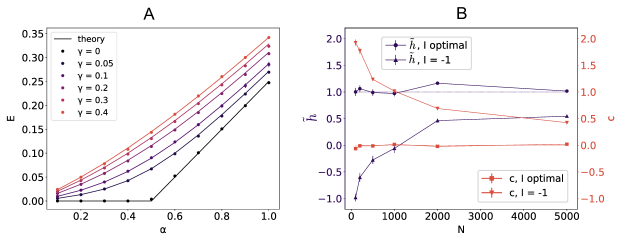
Figure 2: Critical capacity and weight balance. A: Average loss $\left<E\right>$ for a linear perceptron with $f_{E}=0.8$ positive synaptic weights in the case of i.i.d. input $X$ and output $y$ for increasing values of the regularization $\gamma$. Parameters: $N=1000$, $\bar{x}_{E}=\bar{x}_{I}=\sigma_{E}=\sigma_{I}=\bar{y}=\sigma_{y}=1$. Each point is an average across $50$ samples. Full lines show the theoretical results. B: Mean-field component $\tilde{h}$ (left axis, purple) and weight-input correlation $c$ (right axis, red) for increasing dimension $N$ in the case where the bias current $b=I\sqrt{N}$ is either learned ($I$ optimal) or fixed at the outset ($I=-1$) for $f_{E}=1$, $\gamma=0.1$, $\alpha=0.8$. Inputs $X$ and output $y$ are time-correlated with un-normalized Gaussian covariance $C$, $\tau=10$ (see text). The remaining parameters are as in A. The asymptotic value $\tilde{h}=\bar{y}=1$ is highlighted by the purple dotted line, the value $c=0$ by the red dotted line as guide for the eye.

For a generic value of the bias current $b$, there are strong deviations from the condition in Eq (2). In Fig 2B, we compare the value of the average output $\bar{y}$ with $\tilde{h}\equiv\sum_{c\in\left\{E,I\right\}}N_{c}\bar{w}_{c}\bar{x}_{c}+b$, and also plot the residual term $c=\frac{1}{NM}\sum_{i\mu}\delta w_{i}x_{i\mu}$, where we decomposed the weight vector components as $w_{i}=\bar{w}_{c}+\delta w_{i}$ for $c\in\left\{E,I\right\}$. The quantity $c$ measures weight-rate correlations which are responsible for the cancelation of the $\mathcal{O}\left(\sqrt{N}\right)$ bias.

The deviation from Eq (2), shown here for a rapidly decaying covariance of the form $C_{\mu\nu}=e^{-\frac{\left|\mu-\nu\right|}{2\tau^{2}}}$, has been previously described in the context of a target-based learning algorithm used to build E-I-separated rate and spiking models of neural circuits capable of solving input/output tasks Ingrosso_training . In this approach, a randomly initialized recurrent networks $n_{T}$ is driven by a low dimensional signal $z$. Its currents are then used as targets to train the synaptic couplings of a second (rate or spiking) network $n_{S}$, in such a way that the desired output $z$ can later be linearly decoded from the self-sustained activity of $n_{S}$. Each neuron of $n_{S}$ has to independently learn an input/output mapping from firing rates $x$ to currents $y$, using an on-line sign-constrained least square method. In the presence of an L2 regularization and a constant $b\propto\sqrt{N}$ external current, the on-line learning method typically converges onto a solution for the recurrent synaptic weights for which Eq (2) does not hold. As also shown in Ingrosso_training , in the peculiar case of a self-sustained periodic dynamics (in which case off-diagonal terms of the covariance matrix $C_{\mu\nu}$ do not vanish for large $\mu$ or $\nu$) the two contributions $\tilde{h}$ and $c$ scale approximately like $\sqrt{N}$ and cancel each other to produce an $\mathcal{O}\left(1\right)$ total average output $\bar{y}=\tilde{h}+c$.

Power spectrum and synaptic distribution

The theory developed thus far applies to a generic covariance matrix $C$. To connect the spectral properties of $C$ with the signal dynamics, we further assume the $x_{i\mu}$ to be $N$ independent stationary discrete-time processes. In this case, $C_{\mu\nu}=C\left(\mu-\nu\right)$ is a matrix of Toeplitz type Gray_toeplitz , leading to the following expression for the average minimal energy in the $N\to\infty$ limit:

$$\left<E\right>=\frac{\sigma^{2}_{y}}{2\pi}\int_{0}^{\pi}d\phi\frac{\lambda\left(\phi\right)}{1+\Delta\tilde{q}_{w}\lambda\left(\phi\right)}$$

with $\Delta\tilde{q}_{w}$ given by Eq (4). The function $\lambda\left(\phi\right)$ can be computed exactly in some cases (Methods) and corresponds to the average power spectrum of the $x$ and $y$ stochastic processes. Fig 3 shows two representative input signals with Gaussian and exponential covariance matrix $C$ (Fig 3A) and a comparison between the average power spectrum of the input and the analytical results for the eigenvalue spectrum of the matrix $C$ (Fig 3B). From now on, we use the terms Gaussian or rfb (radial basis function) indistinguishably to denote the un-normalized Gaussian function $C_{\mu\nu}=e^{-\frac{\left(\mu-\nu\right)^{2}}{2\tau^{2}}}$.

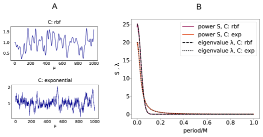
Figure 3: Eigenvalues of $C$ and Fourier spectrum. A: Examples of excitatory input signals $x_{i\mu}$ ($i\in E$) with two different covariance matrices $C$. Top: rbf covariance, $\tau=10$. Bottom: exponential covariance $C_{\mu\nu}=e^{-\frac{\left|\mu-\nu\right|}{\tau}}$, $\tau=10$. Parameters: $\bar{x}_{E}=1$, $\sigma_{E}=0.3$. B: Theoretical eigenvalue spectrum of $C$ with $\tau=10$ versus average power spectrum for positive wave numbers across $N=2000$ independent processes with $M=1000$ time steps.

As shown in Fig 4A in the case of input $x$ and output $y$ with rbf covariance, the squared norm of the optimal synaptic vector $\boldsymbol{w}$ (red curve) is in general a non-monotonic function of $\alpha$, its maximum being attained at bigger values of $\alpha$ as the time constant $\tau$ increases. We also show the minimal energy $E$ and the mean error $\epsilon$ for $\gamma=0.1$. The curves in Fig 4A are the same for any ratio $f_{E}$: the use of an optimal bias current $b$ cancels any asymmetry between E and I populations. For a finite $\gamma$, the average minimal energy $E$ for a given $f_{E}$ decreases as either $\sigma_{E}$ or $\sigma_{I}$ increase. For a given set of parameters $f_{E}$ and $\gamma$, the optimal bias $b$ will in general depend on the load $\alpha$ and the structure of the covariance matrix $C$, as shown in Fig 4B.

Figure 4: Learning temporally structured signals. A: Minimal loss $E$, error $\epsilon$ and norm of the weight vector $\boldsymbol{w}$ as a function of the load $\alpha$ for a linear perceptron trained on a time-correlated signal. Covariance matrix $C$ is of rbf type with $\tau=2$. Parameters: $N=1000$, $f_{E}=0.8$, $\gamma=0.1$, $\bar{x}_{E}=\bar{x}_{I}=\sigma_{E}=\sigma_{I}=\bar{y}=\sigma_{y}=1$. B: Optimal bias $b$ for the two sets of signals with rbf (black curve) and exponential (yellow curve) covariance $C$, with $\tau=2$. Theoretical curves show the value $I\sqrt{N}+\bar{y}$, where $I$ has been computed form the saddle point equations (Methods). Parameters as in A. Each point in A and B is an average across $50$ samples. C: Probability density of non-zero synaptic weights $w_{i}\sqrt{N}$ of a linear perceptron with $N=1000$, a fraction $f_{E}=0.8$ of excitatory weights, trained on $M=600$ exponentially correlated input $x$ and output $y$. The $\delta$ function in zero is omitted for better visualization. Parameters: $\tau=10$, $\gamma=0.1$, $\bar{x}_{E}=\bar{x}_{I}=1$, $\sigma_{I}=2\sigma_{E}=0.4$. The histogram is an average across 50 realizations of input/output signals. Inset: full histogram of synaptic weights $w_{i}\sqrt{N}$.

The probability distribution of the weights $w_{i}$ can easily be derived using the same analytical machinery employed for the calculation of the free-energy $f$ (Methods). For a fixed bias $b$, the probability density of the synaptic weights is composed of two truncated Gaussian distributions with zero mean for the E and I components, plus a finite fraction $p_{0}$ of zero weights, given by

$$p_{0}\left(B\right)=f_{E}H\left(-\eta_{E}B\right)+\left(1-f_{E}\right)H\left(\eta_{I}B\right)$$ (6)

where $H\left(x\right)=\int_{x}^{\infty}dz\frac{e^{-\frac{z^{2}}{2}}}{\sqrt{2\pi}}$, $B$ is an order parameter that must to be computed from the saddle point equations, and $\eta_{c}=\frac{\bar{x}_{c}}{\sigma_{c}}$, with $c\in\left\{E,I\right\}$. Interestingly, the optimal bias $b$ yields the simple results $B=0$, which greatly simplifies the saddle point equations, and implies that half of the synapses are zero, irrespectively of $f_{E}$ and the properties of the covariance matrix $C$. We show in Fig 4D the shape of the optimal weight distribution for a linear perceptron with $80\%$ excitatory synapses, trained on exponentially correlated $x$ and $y$ and with a ratio $\sigma_{I}/\sigma_{E}=2$. It is interesting to note that, in the presence of an optimal external current, both the means of the Gaussian components and the fraction of silent synapses do not depend on the specific properties of input and output signals.

The dynamic properties of input/output mappings affect the shape of the weight distribution in a computable manner. As an example, in a linear perceptron with non-negative synapses, the explicit dependence of the variance of the weights on the input and output auto-correlation time constant is shown in Fig 5A for various loads $\alpha$. Previous work considered an analog perceptron with purely excitatory weights as a model for the graded rate response of Purkinje cells in the cerebellum Clopath_optimal . In the presence of heterogeneity of synaptic properties across cells, a larger variance in their synaptic distribution is expected to be correlated with high frequency temporal fluctuations in input currents. Analogously, the auto-correlation of the typical signals being processed sets the value of the constant external current that a neuron must receive in order to optimize its capacity.

When the input and output have different covariance matrices $C^{x}\neq C^{y}$, a joint diagonalization is not possible in general (Methods). We can nevertheless write an expression (Eq (18)) that holds when input and output patterns are defined on a ring (with periodic boundary conditions) and use it as an approximation for the general case. Fig 5B shows good agreement between numerical experiment and theoretical predictions for the error $\epsilon$ and the squared norm of the synaptic weight vector $\boldsymbol{w}$, when input and output processes have two different time-constants $\tau_{x}$ and $\tau_{y}$.

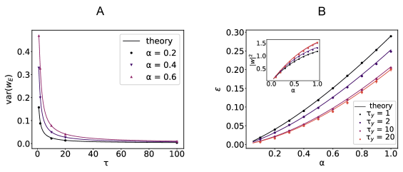
Figure 5: Input/output time constants and learning performance. A: Variance of synaptic weights ($f_{E}=1$) for a linear perceptron of dimension $N=1000$ trained on rbf-correlated signals with increasing time constant $\tau$ for three different values of the load $\alpha$. Parameters: $\gamma=0.1$, $\bar{x}_{E}=\bar{x}_{I}=\sigma_{E}=\sigma_{I}=\bar{y}=\sigma_{y}=1$. B: Average error $\epsilon$ in the case where input and output signals have two different covariance matrices, for increasing time constant $\tau_{y}$ of the output signal $y$. Parameters: $N=1000$, $f_{E}=0.8$, $\gamma=0.1$, $\bar{x}_{E}=\bar{x}_{I}=\bar{y}=\sigma_{y}=1$, $\sigma_{I}=2\sigma_{E}=0.6$, $C^{x}$ rbf with $\tau_{x}=1$, $C^{y}$ rbf with various values of $\tau_{y}$. Inset: norm of the weight vector $\boldsymbol{w}$. Full lines show analytical results. Points are averages across $50$ samples.

Sample covariance and dimensionality

In the discussion thus far, we assumed independence across the “spatial” index $i$ in the input. It is often the case for input signals to be confined to a manifold of dimension smaller than $N$, a feature that can be described by various dimensionality measures, some of which rely on principal component analysis abbott_interactions ; LitwinKumar_optimal . In order to relax the independence assumption, we build on a framework originally introduced in the theory of spin glasses with orthogonal couplings Marinari_replicafield ; Parisi_orthogonal ; Cherrier_interactionmatrix and further developed in the context of adaptive TAP equations Opper_tractable ; Opper_adaptive ; Opper_expectation . Following previous work in the context of information theory of linear vector channels and binary perceptrons Takeda_cdma ; Kabashima_unified ; Shinzato_learning ; Shinzato_Revisited , we employ an expression for an ensemble of rectangular random matrices.

Let us write the input matrix $\left(X\right)_{i\mu}=\bar{x}_{i}+\sigma_{i}\xi_{i\mu}$, with $\xi=USV^{T}$, $S$ being the matrix of singular values. To analyze the properties of the typical case, we start from a generic singular value distribution $S$ and consider i.i.d. output $y_{\mu}$. In calculating the cumulant generating function $Z_{\xi,\delta y}$, we perform a homogeneous average across the left and right principal components $U$ and $V$. Calling $\rho_{\xi\xi^{T}}\left(\lambda\right)$ the eigenvalue distribution of the sample covariance matrix $\xi\xi^{T}$, we can express $Z_{\xi,\delta y}$ in terms of a function $\mathcal{G}_{\xi,\delta y}$ of an enlarged set of overlap parameters, which depends on the so called Shannon transform Tulino_RandomMatrix of $\rho_{\xi\xi^{T}}\left(\lambda\right)$, a quantity that measures the capacity of linear vector channels. The resulting self-consistent equations, which describe the statistical properties of the synaptic weights $w_{i}$, are expressed in terms of the Stieltjes transform of $\rho_{\xi\xi^{T}}\left(\lambda\right)$, an important tool in random matrix theory Tao_topics .

We show the validity of the mean-field approach by employing two different data models for the input signals. In the first example, valid for $\alpha\leq 1$, all the $M$ vectors $\boldsymbol{\xi}_{\mu}$ are orthogonal to each other. This yields an eigenvalue distribution of the simple form $\rho\left(\lambda\right)=\alpha\delta\left(\lambda-1\right)+\left(1-\alpha\right)\delta\left(\lambda\right)$, for which the function $\mathcal{G}_{\xi,\delta y}$ can be computed explicitly Shinzato_Revisited . Additionally, we use a synthetic model where we explicitly set the singular value spectrum of $\xi$ to be $s\left(\alpha\right)=\chi e^{-\frac{\alpha^{2}}{2\sigma_{x}^{2}}}$, with $\chi$ a normalization factor ensuring matrix $\xi$ has unit variance. The shape of the singular value spectrum $s$ controls the spread of the data points $\boldsymbol{\xi}_{\mu}$ in the $N$-dimensional input space, as shown in Figure 6A. As shown in Figure 6B for i.i.d Gaussian output, learning degrades as $\sigma_{x}$ decreases, since inputs tend to be confined to a lower dimensional subspace rather than being equally distributed along input dimensions.

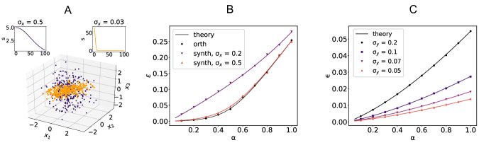
Figure 6: Sample-based PCA and learning performance. A: First three components of inputs $\boldsymbol{\xi}_{\mu}$ with Gaussian singular value spectrum $s$ for two different values of $\sigma_{x}$ (color coded top panels). Parameters: $N=100$, $M=300$. B: Average error $\epsilon$ for three different singular value spectra of the input sample covariance matrix: orthogonal model and Gaussian model with increasing $\sigma_{x}$ (see main text for definition of $\sigma_{x}$). Outputs are i.i.d Gaussian. Parameters: $N=1000$, $f_{E}=0.8$, $\gamma=0.1$, $\bar{x}_{E}=\bar{x}_{I}=\bar{y}=\sigma_{y}=1$, $\sigma_{I}=2\sigma_{E}=0.6$. B: Average error $\epsilon$ for input with orthogonal-type covariance and output $y$ with rbf-type covariance with decreasing $\sigma_{y}$ (see main text for the definition of $\sigma_{y}$). All remaining parameters as in A. Full lines show analytical results. Points are averages across $50$ samples.

For $N$ large enough (in practice, for $N\gtrsim 500$), the statistics of single cases is well captured by the equations for the average case (self-averaging effect). To get a mean-field description for a single case, where a given input matrix $X$ is used, we further assume we have access to the linear expansion $c_{\mu}$ of the output $y$ in the set $\{\boldsymbol{v}_{\mu}\}$ of the columns of the $V$ matrix, namely $\boldsymbol{y}=\bar{y}+\sigma_{y}V\boldsymbol{c}$. The calculation can be carried out in a similar way and yields, for the average regression loss, the following result:

$$\left<E\right>=\frac{\alpha}{2}\sigma_{y}^{2}\tilde{\Lambda}_{w}\left\langle\frac{\lambda^{y}}{\lambda^{x}+\tilde{\Lambda}_{w}}\right\rangle_{\lambda^{x},\lambda^{y}}$$ (7)

The average in Eq (7) is computed over the eigenvalues $\lambda^{x}$ of the sample covariance matrix, which correspond to the PCA variances, and $\lambda^{y}_{\mu}=c_{\mu}^{2}$ (Methods). The quantity $\tilde{\Lambda}_{w}$ can be computed from a set of self-consistent equations that link the order parameter $\Delta\tilde{q}_{w}$ and the first two moments of the synaptic distribution. To better understand the role of the parameter $\tilde{\Lambda}_{w}$, it is instructive to compare Eq (7) with the corresponding result for unconstrained weights, which can be derived from the pseudo-inverse solution (Methods), $w^{*}=\left(\xi\xi^{T}+\gamma\right)^{-1}\xi y$. The average loss is:

$$\left<E\right>=\frac{\alpha}{2}\sigma_{y}^{2}\gamma\left\langle\frac{\lambda^{y}}{\lambda^{x}+\gamma}\right\rangle_{\lambda^{x},\lambda^{y}}$$ (8)

Comparing Eq (7) and Eq (8), we find that $\tilde{\Lambda}_{w}$ acts as an implicit regularization in the sign-constrained case. In Fig 6C, we show results when the dimensionality of the output $y$ along the (temporal) components of the input is modulated by taking $c\left(\alpha\right)=e^{-\frac{\alpha^{2}}{2\sigma_{y}^{2}}}$. The perceptron performance improves as the output signals spreads out across multiple components $\boldsymbol{v}_{\mu}$. The case of i.i.d. output is recovered by taking $c_{\mu}=1$.

Discussion

In this work, I investigated the properties of optimal solutions of a linear perceptron with sign-constrained synapses and correlated input/output signals, thus providing a general mean-field theory for constrained regression in the presence of correlations. I treated both cases where ensemble covariances are known and where the sample covariance is given for a typical case. The latter approach, built on a rotationally invariant assumption, allowed to link the regression performance to the input and output statistical properties expressed by principal component analysis.

I provided the general expression of the weight distribution for regularized regression and found that half of the weights are set to zero, irrespectively of the fraction of excitatory weights, provided the bias is optimized. The shape of the synaptic distribution has been previously described in the binary perceptron with independent input at critical capacity, as well as in the theory of compressed sensing Ganguli_compressed . I elucidated the role of the optimal bias current and its relation to the optimal capacity and the scaling of the solution weights. This analysis also shed light on the structural properties of synaptic matrices which emerge when target-based methods are used for building biologically plausible functional models of rate and spiking networks.

The theory presented in this work is relevant in the effort of establishing quantitative comparisons between the synaptic profile of neural circuits involved in temporal processing of dynamic signals, such as the cerebellum Marr_cerebellar ; Wolpert_cerebellum ; Herzfeld_purkinje , and normative theories that take into account the temporal and geometrical complexity of computational tasks. On the other hand, the construction of progressively more biologically plausible models of neural circuits calls for normative theories of learning in heterogeneous networks, which can be coupled to dynamic mean-field analysis of E-I separated circuits KadmonSompolinsky ; HarishHanselAsynchronous ; mastrogiuseppeeinetworks .

The importance of a theory of constrained regression with realistic input/output statistics goes beyond the realm of neuroscience. Non-negativity is commonly required to provide interpretable results in a wide variety of inference and learning problems. Off-line and on-line least-square estimation methods Chen_nonnegative ; Nascimento_rls are also of great practical importance in adaptive control applications, where constraints on the parameter range are usually imposed by physical plausibility.

In this work, I assumed statistical independence between inputs and outputs. For the sake of biological plausibility, it would be interesting to consider more general input-output correlations for regression and binary discrimination tasks. The classical model for such correlations is provided by the so-called teacher-student (TS) approach Engel_statistical , where the output $y$ is generated by a deterministic parameter-dependent transformation of the input $x$, with a structure similar to the trained neural architecture. The problem of input/output correlations is deeply related to the issue of optimal random nonlinear expansion both in statistical learning theory mei_generalization ; Gerace_generalisation and theoretical neuroscience Babadi_sparseness ; LitwinKumar_optimal , with a history dating back to the Marr-Albus theory of pattern separation in cerebellum Cayco_patternseparation . In a recent work, goldt_modelling introduced a promising generalization of TS, in which labels are generated via a low-dimensional latent representation, and it was shown that this model captures the training dynamics in deep networks with real world datasets.

A general analysis that fully takes into account spatio-temporal correlations in network models could shed light on the emergence of specific network motifs during training. In networks with non-linear dynamics, the mathematical treatment quickly gets challenging even for simple learning rules. In recent years, interesting work has been done to clarify the relation between learning and network motifs, using a variety of mean-field approaches. Examples are the study of associative learning in spin models Brunel_cortical and the analysis of motif dynamics for simple learning rules in spiking networks Ocker_motifs . Incorporating both the temporal aspects of learning and neural cross-correlations in E-I separated models with realistic input/output structure is an interesting topic for future work.

Methods

Replica formalism: ensemble covariance matrix

Using the Replica formalism Mezard_SpinGlassBeyond , the free energy density is written as:

$$-\beta f=\frac{1}{N}\lim_{n\to 0}\frac{\partial}{\partial n}\log\left\langle Z^{n}\right\rangle_{x,y}$$ (9)

The function $Z^{n}$ can be computed by considering a finite number $n$ of replicas of the vector $\boldsymbol{w}$ and subsequently taking a continuation $n\in\mathbb{R}$. In the large $N$ limit, $f$ can be written as the sum of two contributions $-\beta f=\mathcal{G_{S}}+\alpha\mathcal{G}_{E}$, respectively called entropic and energetic part, which depend on a small set of order parameters, to be determined by solving the saddle point equations arising from the expression $\left\langle Z^{n}\right\rangle_{x,y}=e^{-\beta Nf}$ in the limit $n\to 0$. In the following, we will usually drop the subscript in the average $\left\langle\cdot\right\rangle_{x,y}$. To simplify the formulas, we introduce the $\mathcal{O}\left(1\right)$ weights $J_{i}=\sigma_{i}\sqrt{N}w_{i}$. In terms of these rescaled variables, the loss function in Eq (1) takes the form:

$$E\left(\boldsymbol{w};\gamma,\xi,y\right)=\frac{1}{2}\sum_{\mu=1}^{M}\left(\sum_{i=1}^{N}\frac{J_{i}}{\sqrt{N}}\xi_{i\mu}+\frac{1}{\sqrt{N}}\sum_{i=1}^{N}\frac{\bar{x}_{i}}{\sigma_{i}}J_{i}+I\sqrt{N}-y_{\mu}\right)^{2}+\frac{\gamma}{2}\sum_{i=1}^{N}\frac{J_{i}^{2}}{\sigma_{i}^{2}}$$ (10)

by virtue of $x_{i\mu}=\bar{x}_{i}+\sigma_{i}\xi_{i\mu}$. We proceed by inserting the definitions $M^{a}=\frac{1}{\sqrt{N}}\sum_{i=1}^{N}\frac{\bar{x}_{i}}{\sigma_{i}}J_{i}+I\sqrt{N}$ and $\Delta_{\mu a}=\sum_{i=1}^{N}\xi_{i\mu}\frac{J_{ia}}{\sqrt{N}}-\sigma_{y}\delta y_{\mu}$ with the aid of appropriate $\delta$ functions. Assuming balance, namely $M^{a}=\bar{y}$, the averaged replicated partition function $\left\langle Z^{n}\right\rangle$ is:

$$\left\langle Z^{n}\right\rangle =\int\prod_{a}d\mu\left(\boldsymbol{w}_{a}\right)\int\prod_{\mu a}\frac{d\Delta_{\mu a}du_{\mu a}}{2\pi}Z_{\xi,\delta y}$$

$$e^{\sum_{a}\hat{M}^{a}\left(\sqrt{N}M^{a}-\sum_{i}\frac{\bar{x}_{i}}{\sigma_{i}}J_{i}-NI\right)-i\sum_{\mu a}u_{\mu a}\Delta_{\mu a}-\frac{\beta}{2}\sum_{\mu a}\Delta_{\mu a}^{2}-\frac{\beta\gamma}{2}\sum_{ia}\frac{J_{ia}^{2}}{\sigma_{i}^{2}}}$$ (11)

where:

$$Z_{\xi,\delta y}=\left\langle e^{i\sum_{\mu a}u_{\mu a}\left(\sum_{i}\xi_{i\mu}\frac{J_{ia}}{\sqrt{N}}-\sigma_{y}\delta y_{\mu}\right)}\right\rangle_{\xi,\delta y}$$ (12)

The calculation can be carried out by introducing overlap order parameters $Nq_{w}^{ab}=\sum_{i=1}^{N}J_{ia}J_{ib}$ with the use of $n\left(n-1\right)/2$ additional $\delta$ functions, together with their conjugate variables $\hat{q}^{ab}_{w}$. Owing to the convexity of the regression problem, we use a Replica Symmetry (RS) Mezard_SpinGlassBeyond ansatz $q_{w}^{ab}=q_{w}+\delta_{ab}\Delta q_{w}$, and correspondingly for the conjugate parameters. Additionally, we will take $M^{a}=M$ and $\hat{M}^{a}=\hat{M}$.

Entropic part

The total volume of configurations $\boldsymbol{w}_{a}$ for fixed values of the overlap parameters is given by the entropic part, which can be computed at RS level by standard methods, yielding:

$$\mathcal{G}_{S} =\sum_{c\in\left\{E,I\right\}}f_{c}\int Dz\log\int_{0}^{\infty}dJe^{-\frac{J^{2}}{2}\left(\Delta\hat{q}_{w}+\frac{\beta\gamma}{\sigma_{c}^{2}}\right)+s_{c}\left(z\sqrt{\hat{q}_{w}}-\eta_{c}\hat{M}\right)J}$$

$$-\hat{M}I+\frac{\Delta\hat{q}_{w}}{2}\left(\Delta q_{w}+q_{w}\right)-\frac{\hat{q}_{w}\Delta q_{w}}{2}$$ (13)

where $Dz=\frac{e^{-\frac{z^{2}}{2}}}{\sqrt{2\pi}}$. In Eq (13), we introduced the notations $f_{I}=1-f_{E}$ and $s_{E}=-s_{I}=1$.

Energetic part

In order to compute the energetic part, we first need to evaluate the average with respect to $\xi$ and $\delta y$ in Eq (12). Performing the two Gaussian integrals we get:

$$Z_{\xi,\delta y}=e^{-\frac{1}{2}\sum_{\mu\nu}\sum_{ab}q_{w}^{ab}u_{\mu a}u_{\nu b}C_{\mu\nu}^{x}-\frac{\sigma_{y}^{2}}{2}\sum_{\mu\nu}\sum_{ab}u_{\mu a}u_{\nu b}C_{\mu\nu}^{y}}$$ (14)

from which:

$$e^{\alpha N\mathcal{G}_{E}} \propto\int\prod_{\mu a}\frac{d\Delta_{\mu a}du_{\mu a}}{2\pi}e{}^{-\frac{\beta}{2}\sum_{\mu a}\Delta_{\mu a}^{2}-\frac{1}{2}\sum_{\mu\nu}\sum_{ab}q_{w}^{ab}u_{\mu a}u_{\nu b}C_{\mu\nu}^{x}}$$

$$e^{-\frac{\sigma_{y}^{2}}{2}\sum_{\mu\nu}\sum_{ab}u_{\mu a}u_{\nu b}C_{\mu\nu}^{y}-i\sum_{\mu a}u_{\mu a}\Delta_{\mu a}}$$ (15)

In the special case $C^{x}=C^{y}\equiv C$, we can jointly rotate the $u$’s and $\Delta$’s variables, using $C=V\Lambda V^{T}$, to obtain:

$$e^{\alpha N\mathcal{G}_{E}} \propto\int\prod_{\mu a}\frac{d\Delta_{\mu a}du_{\mu a}}{2\pi}e^{-\frac{\beta}{2}\sum_{\mu a}\Delta_{\mu a}^{2}-\frac{1}{2}\sum_{\mu}\sum_{ab}q_{w}^{ab}u_{\mu a}u_{\mu b}\lambda_{\mu}}$$

$$e^{-\frac{\sigma_{y}^{2}}{2}\sum_{\mu}\sum_{ab}u_{\mu a}u_{\mu b}\lambda_{\mu}-i\sum_{\mu a}u_{\mu a}\Delta_{\mu a}}$$ (16)

Within the RS ansatz, we get:

$$\mathcal{G}_{E}=-\frac{1}{2}\left\langle\log\left(1+\beta\Delta q_{w}\lambda\right)\right\rangle_{\lambda}-\frac{\beta}{2}\left(q_{w}+\sigma_{y}^{2}\right)\left\langle\frac{\lambda}{1+\beta\Delta q_{w}\lambda}\right\rangle_{\lambda}$$ (17)

The brakets $\left\langle\right\rangle_{\lambda}$ in Eq (17) stand for an average over the eigenvalue distribution $\rho\left(\lambda\right)$ of $C$ in the $N\to\infty$ limit, assuming self-averaging Monasson_properties ; Tarkowski_optimal . When $C^{x}\neq C^{y}$, we can derive a similar expression under the assumption of a ring topology in pattern space (corresponding to period boundary conditions in the index $\mu$). In the main text, we show that the expression

$$\alpha\mathcal{G}_{E}=-\frac{1}{2N}\sum_{\mu}\log\left(1+\beta\Delta q_{w}\lambda_{\mu}^{x}\right)-\frac{\beta}{2N}\sum_{\mu}\frac{q_{w}\lambda_{\mu}^{x}+\sigma^{2}_{y}\lambda_{\mu}^{y}}{1+\beta\Delta q_{w}\lambda_{\mu}^{x}}$$ (18)

yields good results also when $C^{x}$ and $C^{y}$ are covariance matrices of stationary discrete-time processes.

Saddle point equations

All in all, the free-energy is:

$$-\beta f =-\hat{M}I+\frac{\Delta\hat{q}_{w}}{2}\left(\Delta q_{w}+q_{w}\right)-\frac{\hat{q}_{w}\Delta q_{w}}{2}$$

$$-\frac{1}{2N}\sum_{\mu}\log\left(1+\beta\Delta q_{w}\lambda_{\mu}^{x}\right)-\frac{\beta}{2N}\sum_{\mu}\frac{q_{w}\lambda_{\mu}^{x}+\sigma_{y}^{2}\lambda_{\mu}^{y}}{1+\beta\Delta q_{w}\lambda_{\mu}^{x}}+$$

$$\sum_{c\in\left\{E,I\right\}}f_{c}\int Dz\log\int_{0}^{\infty}dJe^{-\frac{J^{2}}{2}\left(\Delta\hat{q}_{w}+\frac{\beta\gamma}{\sigma_{c}^{2}}\right)+s_{c}\left(z\sqrt{\hat{q}_{w}}-\eta_{c}\hat{M}\right)J}$$ (19)

The equations stemming from the entropic part can be written as:

$$q_{w}=\left\langle\left\langle J\right\rangle_{J}^{2}\right\rangle_{z}$$ (20)

$$\Delta q_{w}=\left\langle\left\langle J^{2}\right\rangle_{J}\right\rangle_{z}-\left\langle\left\langle J\right\rangle_{J}^{2}\right\rangle_{z}$$ (21)

$$I+\sum_{c\in\left\{E,I\right\}}\eta_{c}\left\langle\left\langle J\right\rangle_{J}\right\rangle_{z}=0$$ (22)

where the averages $\left\langle\,\right\rangle_{J}$ and $\left\langle\,\right\rangle_{z}$ in Eq (20), (21), (22) are taken with respect to the mean-field distribution of the $J$ weights:

$$p\left(J;z\right) \propto\sum_{c\in\left\{E,I\right\}}f_{c}p_{c}\left(J;z\right)$$ (23)

$$p_{c}\left(J;z\right) \propto\theta\left(s_{c}J\right)e^{-\frac{J^{2}}{2}\left(\Delta\hat{q}_{w}+\frac{\beta\gamma}{\sigma_{c}}\right)+J\left(z\sqrt{\hat{q}_{w}}-\eta_{c}\hat{M}\right)}$$ (24)

where $z$ is a standard normal variable and $\theta$ is the Heaviside function: $\theta\left(x\right)=1$ when $x>0$ and $0$ otherwise. In the $\beta\to\infty$ limit, the unicity of solution for $\gamma>0$ implies that $\Delta q_{w}\to 0$. We therefore use the following scalings for the order parameters:

$$\beta\Delta q_{w}=\Delta\tilde{q}_{w}$$ (25)

$$\hat{q}_{w}=\beta^{2}C$$ (26)

$$\Delta\hat{q}_{w}=\beta A$$ (27)

$$\hat{M}=\beta B\sqrt{C}$$ (28)

while $q_{w}=\mathcal{O}\left(1\right)$. In this scaling, Eq (20), (21), (22) take the form:

$$\frac{q_{w}}{C}=\sum_{c\in\left\{E,I\right\}}\frac{f_{c}}{\left(A+\frac{\gamma}{\sigma_{c}^{2}}\right)^{2}}\left(\left(1+\eta_{c}^{2}B^{2}\right)H\left(s_{c}\eta_{c}B\right)-s_{c}\eta_{c}BG\left(\eta_{c}B\right)\right)$$ (29)

$$\Delta\tilde{q}_{w}=\sum_{c\in\left\{E,I\right\}}\frac{f_{c}}{A+\frac{\gamma}{\sigma_{c}^{2}}}H\left(s_{c}\eta_{c}B\right)$$ (30)

$$\frac{I}{\sqrt{C}}=\sum_{c\in\left\{E,I\right\}}\frac{f_{c}}{A+\frac{\gamma}{\sigma_{c}^{2}}}\left(\eta_{c}^{2}BH\left(s_{c}\eta_{c}B\right)-s_{c}\eta_{c}G\left(\eta_{c}B\right)\right)$$ (31)

where $G\left(z\right)=\frac{e^{-\frac{z^{2}}{2}}}{\sqrt{2\pi}}$. The squared norm of the weights $v=\sum_{i=1}^{N}w_{i}^{2}$ is given by $v=2\partial_{\gamma}f$:

$$v=C\sum_{c\in\left\{E,I\right\}}\frac{f_{c}}{\sigma_{c}^{2}\left(A+\frac{\gamma}{\sigma_{c}^{2}}\right)^{2}}\left(\left(1+\eta_{c}^{2}B^{2}\right)H\left(s_{c}\eta_{c}B\right)-s_{c}\eta_{c}BG\left(\eta_{c}B\right)\right)$$ (32)

In the $\beta\to\infty$, it can be easily shown that the mean-field weight probability density of the rescaled weights $\sqrt{N}w_{i}$ is a superposition of a $\delta$ function in zero and two truncated Gaussian densitites:

$$p\left(\sqrt{N}w\right)=p_{0}\left(B\right)\delta\left(w\right)+\sum_{c}f_{c}G\left(\sqrt{N}w;M_{c},\Sigma_{c}\right)\theta\left(s_{c}J\right)$$ (33)

where the mean and standard deviation of the Gaussians $G\left(\cdot;M,\Sigma\right)$ are:

$$M_{c}=-\frac{\eta_{c}B\sqrt{C}}{\sigma_{c}A+\frac{\gamma}{\sigma_{c}}},$$ (34)

$$\Sigma_{c}=\frac{\sqrt{C}}{\sigma_{c}A+\frac{\gamma}{\sigma_{c}}}$$ (35)

The fraction of zero weights is given by:

$$p_{0}\left(B\right)=f_{E}H\left(-\eta_{E}B\right)+\left(1-f_{E}\right)H\left(\eta_{I}B\right)$$

where $H\left(x\right)=\int_{x}^{\infty}Dz$. The two remaining saddle point equations are:

$$C=\frac{1}{N}\sum_{\mu}\lambda_{\mu}^{x}\frac{q_{w}\lambda_{\mu}^{x}+\sigma_{y}^{2}\lambda_{\mu}^{y}}{\left(1+\Delta\tilde{q}_{w}\lambda_{\mu}^{x}\right)^{2}}$$ (36)

$$A=\frac{1}{N}\sum_{\mu}\frac{\lambda_{\mu}^{x}}{1+\Delta\tilde{q}_{w}\lambda_{\mu}^{x}}$$ (37)

Optimizing $f$ with respect to the bias $b=I\sqrt{N}$ immediately implies $B=0$, by virtue of Eq (28). Using the scaling assumptions Eq (25)-(28) together with the saddle point Eq (30)-(37), we get Eq (4) in the main text, that is valid for any $\alpha$ for $\gamma>0$. In the unregularized case ($\gamma=0$), it describes solutions in the error regime $\alpha>\alpha_{c}$. The optimal bias $b$ can be computed by $I\sqrt{N}$ using Eq (31), that is valid up to the an $\mathcal{O}\left(1\right)$ term equal to $\bar{y}$ (Fig 4B). The expression for the average minimal energy is:

$$\left<E\right>=\frac{\sigma_{y}^{2}}{2N}\sum_{\mu}\frac{\lambda_{\mu}^{y}}{1+\Delta\tilde{q}_{w}\lambda_{\mu}^{x}}$$ (38)

Spectrum of exponential and rbf covariance

For the exponential covariance $C_{\mu\nu}=e^{-\frac{\left|\mu-\nu\right|}{\tau}}$ one has:

$$\lambda\left(\phi\right)=\frac{1-x^{2}}{1-2x\cos\phi+x^{2}}$$

with $x=e^{-\frac{1}{\tau}}$. In the rbf case $C_{\mu\nu}=e^{-\frac{\left|\mu-\nu\right|^{2}}{2\tau^{2}}}$, the spectrum is:

$$\lambda\left(\phi\right)=\vartheta_{3}\left(\frac{\phi}{2},e^{-\frac{1}{2\tau^{2}}}\right)$$

with $\vartheta_{3}\left(z,q\right)=1+2\sum_{n=1}^{\infty}q^{n^{2}}\cos\left(2nz\right)$ the Jacobi theta function of 3rd type.

Replica formalism: sample covariance matrix

In the case of a sample covariance matrix, the free-energy is a sum of three contributions $-\beta f=\mathcal{G_{S}}+\mathcal{G}_{\xi,\delta y}+\alpha\mathcal{G}_{E}$. The entropic part is unchanged. As explained in the main text, we extend the calculations in Shinzato_learning ; Shinzato_Revisited to the case where the linear expansion of $y_{\mu}$ on the right singular vectors $V_{\cdot\mu}$ is known, by taking $\delta y_{\mu}=\sum_{\nu}V_{\mu\nu}c_{\nu}$. Using again the expressions $\left(X\right)_{i\mu}=\bar{x}_{i}+\sigma_{i}\xi_{i\mu}$ and $\xi=USV^{T}$, the replicated cumulant generating function for the joint (mean-removed) input and output is:

$$Z_{\xi,\delta y} =\left\langle\exp\left(i\sum_{a}\tilde{\boldsymbol{J}}_{a}^{T}S\tilde{\boldsymbol{u}}_{a}-i\sigma_{y}\boldsymbol{c}^{T}\sum_{a}\tilde{\boldsymbol{u}}_{a}\right)\right\rangle_{p\left(\tilde{\boldsymbol{J}}_{a},\tilde{\boldsymbol{u}}_{a}\right)}$$ (39)

where we used the change of variables $\tilde{J}_{ia}=\sum_{k}U_{ki}J_{ka}$ and $\tilde{u}_{\mu a}=\sum_{k}V_{k\mu}u_{ka}$. The average in Eq (39) is taken over the joint distribution $p\left(\tilde{\boldsymbol{J}}_{a},\tilde{\boldsymbol{u}}_{a}\right)$ resulting from averaging over the Haar measure on the orthogonal matrices $U$ and $V$. For a single replica, $Z_{\xi,\delta y}$ will only depend on the squared norms $Q_{w}=\sum_{i}\frac{\tilde{J}_{i}^{2}}{N}$ and $Q_{u}=\sum_{\mu}\frac{\tilde{u}_{\mu}^{2}}{M}$ of the two vectors $\tilde{\boldsymbol{J}}$ and $\tilde{\boldsymbol{u}}$. We can therefore write the average in the following way:

$$\left\langle\exp\left(i\tilde{\boldsymbol{J}}^{T}S\tilde{\boldsymbol{u}}-i\sigma_{y}\boldsymbol{c}^{T}\tilde{\boldsymbol{u}}\right)\right\rangle_{p\left(\tilde{\boldsymbol{J}},\tilde{\boldsymbol{u}}\right)}\propto\int\delta\left(\left|\tilde{\boldsymbol{J}}\right|^{2}-NQ_{w}\right)\delta\left(\left|\tilde{\boldsymbol{u}}\right|^{2}-MQ_{u}\right)e^{i\tilde{\boldsymbol{J}}^{T}S\tilde{\boldsymbol{u}}-i\sigma_{y}\boldsymbol{c}^{T}\tilde{\boldsymbol{u}}}$$ (40)

Introducing Fourier representation for the $\delta$ functions, we are left with an expression involving an $N+M$ dimensional Gaussian integral:

$$\int\frac{d\Lambda_{w}}{4\pi i}\frac{d\Lambda_{u}}{4\pi i}e^{\frac{N\Lambda_{w}Q_{w}}{2}+\frac{M\Lambda_{u}Q_{u}}{2}}\int d\tilde{\boldsymbol{J}}d\tilde{\boldsymbol{u}}e^{-\frac{\Lambda_{w}}{2}\left|\tilde{\boldsymbol{J}}\right|^{2}-\frac{\Lambda_{u}}{2}\left|\tilde{\boldsymbol{u}}\right|^{2}+i\tilde{\boldsymbol{J}}^{T}S\tilde{\boldsymbol{u}}-i\sigma_{y}\boldsymbol{c}^{T}\tilde{\boldsymbol{u}}}$$

$$=\frac{\left(2\pi\right)^{\frac{N+M}{2}}}{\left(4\pi i\right)^{2}}\int d\Lambda_{w}d\Lambda_{u}e^{\frac{N\Lambda_{w}Q_{w}}{2}+\frac{M\Lambda_{u}Q_{u}}{2}}\det\mathcal{M}{}^{-\frac{1}{2}}\exp\left(-\frac{\sigma_{y}^{2}}{2}\left(\begin{array}[]{cc}\boldsymbol{0}&\boldsymbol{c}\end{array}\right)\mathcal{M}^{-1}\left(\begin{array}[]{c}\boldsymbol{0}\\ \boldsymbol{c}\end{array}\right)\right)$$ (44)

where

$$\mathcal{M}=\left(\begin{array}[]{cc}\Lambda_{w}{\mathds{1}}_{N}&-iS\\ -iS^{T}&\Lambda_{u}{\mathds{1}}_{M}\end{array}\right)$$

and ${\mathds{1}}_{K}$ is the identity matrix of dimension $K$. Following Shinzato_Revisited , the determinant can be easily calculated:

$$\frac{1}{N}\log\det\mathcal{M} =\frac{1}{N}\sum_{k=1}^{\min\left(N,M\right)}\log\left(\lambda_{k}^{x}+\Lambda_{w}\Lambda_{u}\right)+\frac{\left(N-\min\left(N,M\right)\right)}{N}\log\Lambda_{u}\to$$ (45)

$$\to\left\langle\log\left(\lambda_{k}^{x}+\Lambda_{w}\Lambda_{u}\right)\right\rangle_{\lambda^{x}}+\left(\alpha-1\right)\log\Lambda_{u}$$ (46)

where the limit is taken for $N\to\infty$ and the average is with respect to the eigenvalue distribution $\rho\left(\lambda^{x}\right)$. As for the quadratic portion of the Gaussian integral, calling $\lambda_{k}^{y}=c_{k}^{2}$, we will use the shorthand

$$\left\langle\frac{\lambda^{y}}{\lambda^{x}+\Lambda_{w}\Lambda_{u}}\right\rangle_{\lambda^{x},\lambda^{y}}\equiv\frac{\Lambda_{w}}{M}\sum_{k=1}^{\Omega}\frac{\lambda_{k}^{y}}{\lambda^{x}_{k}+\Lambda_{w}\Lambda_{u}}+\frac{\left(M-\Omega\right)}{M}\sum_{k=M+1}^{\Omega}\frac{\lambda_{k}^{y}}{\Lambda_{w}}$$

where $\Omega=\max\left(N,M\right)$. Considering now the replicated generating function, all the $n\left(2n-1\right)$ cross-product $\boldsymbol{J}_{a}\cdot\boldsymbol{J}_{b}=\tilde{\boldsymbol{J}}_{a}\cdot\tilde{\boldsymbol{J}}_{b}$ and $\boldsymbol{u}_{a}\cdot\boldsymbol{u}_{b}=\tilde{\boldsymbol{u}}_{a}\cdot\tilde{\boldsymbol{u}}_{b}$ must be conserved via the multiplication of $U$ and $V$. Together with the overlap parameters $Nq^{ab}_{w}=\sum_{i}J_{ia}J_{ib}$, we additionally introduce the quantities $Mq_{u}^{ab}=\sum_{\mu}u_{\mu a}u_{\mu b}$. In the RS case, we again take: $q_{w}^{ab}=q_{w}+\delta_{ab}\Delta q_{w}$ and, similarly for the $u$’s, $q_{u}^{ab}=-q_{u}+\delta_{ab}\Delta q_{u}$. In the basis where both $q_{w}^{ab}$ and $q^{ab}_{u}$ are diagonal, the expression becomes

$$Z_{\xi,\delta y}=\left<e^{i\tilde{\boldsymbol{J}}_{1}^{T}S\tilde{\boldsymbol{u}}_{1}-i\sigma_{y}\boldsymbol{c}^{T}\sqrt{n}\tilde{\boldsymbol{u}}_{1}}\prod_{b=2}^{n}e^{i\tilde{\boldsymbol{J}}_{b}^{T}S\tilde{\boldsymbol{u}}_{b}}\right>$$ (47)

so in the limit $n\to 0$ we have:

$$2\mathcal{G}_{\xi,\delta y}=F\left(\Delta q_{w},\Delta q_{u}\right)+q_{w}\frac{\partial F\left(\Delta q_{w},\Delta q_{u}\right)}{\partial\Delta q_{w}}-q_{u}\frac{\partial F\left(\Delta q_{w},\Delta q_{u}\right)}{\partial\Delta q_{u}}-\alpha\sigma_{y}^{2}K\left(\Lambda_{w},\Lambda_{u}\right)$$ (48)

with the function $F$ given by:

$$F\left(x,y\right) =\mbox{Extr}_{\Lambda_{w},\Lambda_{u}}\left\{-\left\langle\log\left(\lambda^{x}+\Lambda_{w}\Lambda_{u}\right)\right\rangle_{\lambda^{x}}-\left(\alpha-1\right)\log\Lambda_{u}+\Lambda_{w}x+\alpha\Lambda_{u}y\right\}$$

$$-\log x-\alpha\log y-\left(1+\alpha\right)$$ (49)

and $K\left(\Lambda_{w},\Lambda_{u}\right)=\Lambda_{w}\left\langle\frac{\lambda^{y}}{\lambda^{x}+\Lambda_{w}\Lambda_{u}}\right\rangle_{\lambda^{x},\lambda^{y}}$. In Eq (48), it is intended that $\Lambda_{w}$ and $\Lambda_{w}$ are implied by the Legendre Transform conditions:

$$\Delta q_{w}=\Lambda_{u}\left\langle\frac{1}{\lambda^{x}+\Lambda_{w}\Lambda_{u}}\right\rangle_{\lambda^{x}}$$ (50)

$$\alpha\Delta q_{u}=\frac{\alpha-1}{\Lambda_{u}}+\Lambda_{w}\left\langle\frac{1}{\lambda^{x}+\Lambda_{w}\Lambda_{u}}\right\rangle_{\lambda^{x}}$$ (51)

The calculation of the energetic part $\mathcal{G}_{E}$ is standard and gives:

$$2\mathcal{G}_{E}=\Delta\hat{q}_{u}\left(\Delta q_{u}-q_{u}\right)+\hat{q}_{u}\Delta q_{u}-\log\left(1+\beta\Delta\hat{q}_{u}\right)-\beta\frac{\hat{q}_{u}}{1+\beta\Delta\hat{q}_{u}}$$ (52)

Eliminating $\hat{q}_{u}$ and $\Delta\hat{q}_{u}$ at the saddle point in Eq (52), $\mathcal{G}_{E}$ reduces to:

$$\mathcal{G}_{E}=\frac{q_{u}-\Delta q_{u}}{2\beta}-\frac{q_{u}}{2\Delta q_{u}}+\frac{1}{2}\log\Delta q_{u}$$ (53)

Saddle point equations

The entropic saddle point equations are unchanged. The final expression $-\beta f=\mathcal{G_{S}}+\mathcal{G}_{\xi,\delta y}+\alpha\mathcal{G}_{E}$ implies the following saddle point equations:

$$\Delta\hat{q}_{w}+\frac{\partial F}{\partial\Delta q_{w}}=0$$ (54)

$$\frac{\alpha}{\Delta q_{u}}-\frac{\alpha}{\beta}+\frac{\partial F}{\partial\Delta q_{u}}=0$$ (55)

$$\hat{q}_{w}=q_{w}\frac{\partial^{2}F}{\partial\Delta q_{w}^{2}}-q_{u}\frac{\partial^{2}F}{\partial\Delta q_{w}\Delta q_{u}}-\alpha\sigma_{y}^{2}\frac{\partial K}{\partial\Delta q_{w}}$$ (56)

$$\alpha\frac{q_{u}}{\Delta q_{u}^{2}}=q_{u}\frac{\partial^{2}F}{\partial\Delta q_{u}^{2}}-q_{w}\frac{\partial^{2}F}{\partial\Delta q_{w}\Delta q_{u}}+\alpha\sigma_{y}^{2}\frac{\partial K}{\partial\Delta q_{u}}$$ (57)

The saddle point values of the conjugate Legendre variables $\Lambda_{w}$, $\Lambda_{u}$ greatly simplify the expression for the first and second derivatives of $F$. Indeed, from Eq (54), (55) one has:

$$\Lambda_{w}=\frac{1}{\Delta q_{w}}-\Delta\hat{q}_{w}$$ (58)

$$\Lambda_{u}=\beta^{-1}$$ (59)

or, setting $\Lambda_{w}=\beta\tilde{\Lambda}_{w}$:

$$\tilde{\Lambda}_{w}=\frac{1}{\Delta\tilde{q}_{w}}-A$$ (60)

In particular, Eq (50) shows that $\Delta\tilde{q}_{w}$ is expressed by a Stieltjes transform of $\rho\left(\lambda^{x}\right)$ and the first term in Eq (49) is its Shannon transform. In the limit $\beta\to\infty$, using the following additional scaling relations for the $u$ overlaps:

$$q_{u}=\beta^{2}\tilde{q}_{u}$$ (61)

$$\Delta q_{u}=\beta\Delta\tilde{q}_{u}$$ (62)

we get the expression for the energy:

$$\left<E\right>=\frac{\alpha}{2}\sigma_{y}^{2}\tilde{\Lambda}_{w}\left\langle\frac{\lambda^{y}}{\lambda^{x}+\tilde{\Lambda}_{w}}\right\rangle_{\lambda^{x},\lambda^{y}}$$

i.i.d. and unconstrained cases

Either setting $K=0$ of $\lambda^{y}=0$ reverts back to the i.i.d. output case. In the special case of i.i.d. inputs, the eigenvalue distribution is Marchenko-Pastur

$$\rho\left(\lambda\right)=\frac{\text{$\sqrt{\left(\lambda-\lambda_{-}\right)\left(\lambda_{+}-\lambda\right)}$}}{2\pi\lambda}$$ (63)

with $\lambda_{+/-}=\left(1\pm\sqrt{\alpha}\right)^{2}$, from which $F\left(\Delta q_{w},\Delta q_{u}\right)=-\frac{\alpha}{2}\Delta q_{w}\Delta q_{u}$. The saddle point equations are essentially the same as the ones in the previous section with $C_{\mu\nu}^{x}=C_{\mu\nu}^{y}=\delta_{\mu\nu}$.

Let us also note that, in the simple unconstrained case, taking for simplicity $\bar{x}_{i}=0$ and $b=0$, the entropic part can be worked out to be, up to constant terms:

$$2\mathcal{G}_{S}=\log\Delta q_{w}+\frac{q_{w}}{\Delta q_{w}}-\beta\gamma\left(\Delta q_{w}+q_{w}\right)$$ (64)

which, at the saddle point, implies $\tilde{\Lambda}_{w}=\gamma$. The mean-field distribution $p\left(\sqrt{N}w\right)$ is a zero-mean Gaussian with variance $v=q_{w}$. Using the properties of the Hessian of the Legendre Transform, it is easy to show that:

$$q_{w}=\alpha\frac{\partial K}{\partial\Lambda_{w}}=\alpha\left\langle\frac{\lambda^{x}\lambda^{y}}{\left(\lambda^{x}+\gamma\right)^{2}}\right\rangle_{\lambda^{x},\lambda^{y}}$$ (65)

$$\left<E\right>=\frac{\alpha}{2}\sigma_{y}^{2}\gamma\left\langle\frac{\lambda^{y}}{\lambda^{x}+\gamma}\right\rangle_{\lambda^{x},\lambda^{y}}$$ (66)

These expressions can also be derived from the pseudo-inverse solution (we take $\bar{y}=0$ for simplicity) $w^{*}=\left(\xi\xi^{T}+\gamma\right)^{-1}\xi y$ by taking an average across $\xi$ and $y$ in the two expressions:

$$v=\left<w^{*T}w^{*}\right>=\mbox{Tr}\left(\xi yy^{T}\xi^{T}\left(\xi\xi^{T}+\gamma\right)^{-2}\right)$$ (67)

$$\left<E\right>=\frac{1}{2}\left<y^{T}y\right>-\frac{1}{2}\mbox{Tr}\left(\xi yy^{T}\xi^{T}\left(\xi\xi^{T}+\gamma\right)^{-1}\right)$$ (68)

The i.i.d. output case also follows by performing independent averages over $y$ and $\xi$.

- [1] H. Francis Song, Guangyu R. Yang, and Xiao-Jing Wang. Training excitatory-inhibitory recurrent neural networks for cognitive tasks: A simple and flexible framework. PLOS Computational Biology, 12(2):1–30, 02 2016.
- [2] Wilten Nicola and Claudia Clopath. Supervised learning in spiking neural networks with force training. Nature Communications, 8(1):2208, 2017.
- [3] Alessandro Ingrosso and L. F. Abbott. Training dynamically balanced excitatory-inhibitory networks. PLOS ONE, 14(8):1–18, 08 2019.
- [4] Christopher M Kim and Carson C Chow. Learning recurrent dynamics in spiking networks. eLife, 7:e37124, Sep 2018.
- [5] Wieland Brendel, Ralph Bourdoukan, Pietro Vertechi, Christian K. Machens, and Sophie Denève. Learning to represent signals spike by spike. PLOS Computational Biology, 16(3):1–23, 03 2020.
- [6] Nicolas Brunel, Vincent Hakim, Philippe Isope, Jean-Pierre Nadal, and Boris Barbour. Optimal information storage and the distribution of synaptic weights: Perceptron versus purkinje cell. Neuron, 43(5):745 – 757, 2004.
- [7] Boris Barbour, Nicolas Brunel, Vincent Hakim, and Jean-Pierre Nadal. What can we learn from synaptic weight distributions? Trends in Neurosciences, 30(12):622 – 629, 2007.
- [8] Nicolas Brunel. Is cortical connectivity optimized for storing information? Nature Neuroscience, 19(5):749–755, 2016.
- [9] E Gardner. The space of interactions in neural network models. Journal of Physics A: Mathematical and General, 21(1):257–270, Jan 1988.
- [10] Claudia Clopath, Jean-Pierre Nadal, and Nicolas Brunel. Storage of correlated patterns in standard and bistable purkinje cell models. PLoS computational biology, 8(4):e1002448–e1002448, 2012.
- [11] Julio Chapeton, Tarec Fares, Darin LaSota, and Armen Stepanyants. Efficient associative memory storage in cortical circuits of inhibitory and excitatory neurons. Proceedings of the National Academy of Sciences, 109(51):E3614–E3622, 2012.
- [12] Danke Zhang, Chi Zhang, and Armen Stepanyants. Robust associative learning is sufficient to explain the structural and dynamical properties of local cortical circuits. Journal of Neuroscience, 39(35):6888–6904, 2019.
- [13] Ran Rubin, L. F. Abbott, and Haim Sompolinsky. Balanced excitation and inhibition are required for high-capacity, noise-robust neuronal selectivity. Proceedings of the National Academy of Sciences, 114(44):E9366–E9375, 2017.
- [14] H. S. Seung, H. Sompolinsky, and N. Tishby. Statistical mechanics of learning from examples. Phys. Rev. A, 45:6056–6091, Apr 1992.
- [15] Claudia Clopath and Nicolas Brunel. Optimal properties of analog perceptrons with excitatory weights. PLOS Computational Biology, 9(2):1–6, 02 2013.
- [16] H Gutfreund and Y Stein. Capacity of neural networks with discrete synaptic couplings. Journal of Physics A: Mathematical and General, 23(12):2613–2630, Jun 1990.
- [17] Jeffry S. Isaacson and Massimo Scanziani. How inhibition shapes cortical activity. Neuron, 72(2):231 – 243, 2011.
- [18] Rachel E. Field, James A. D’amour, Robin Tremblay, Christoph Miehl, Bernardo Rudy, Julijana Gjorgjieva, and Robert C. Froemke. Heterosynaptic plasticity determines the set point for cortical excitatory-inhibitory balance. Neuron, 2020.
- [19] Guillaume Hennequin, Everton J. Agnes, and Tim P. Vogels. Inhibitory plasticity: Balance, control, and codependence. Annual Review of Neuroscience, 40(1):557–579, 2017. PMID: 28598717.
- [20] Yashar Ahmadian and Kenneth D. Miller. What is the dynamical regime of cerebral cortex? arXiv:1908.10101, 2019.
- [21] C. van Vreeswijk and H. Sompolinsky. Chaos in neuronal networks with balanced excitatory and inhibitory activity. Science, 274(5293):1724–1726, 1996.
- [22] C. van Vreeswijk and H. Sompolinsky. Chaotic balanced state in a model of cortical circuits. Neural Comput., 10(6):1321–1371, Aug 1998.
- [23] Alfonso Renart, Jaime de la Rocha, Peter Bartho, Liad Hollender, Néstor Parga, Alex Reyes, and Kenneth D. Harris. The asynchronous state in cortical circuits. Science, 327(5965):587–590, 2010.
- [24] Jonathan Kadmon and Haim Sompolinsky. Transition to chaos in random neuronal networks. Phys. Rev. X, 5:041030, Nov 2015.
- [25] Omri Harish and David Hansel. Asynchronous rate chaos in spiking neuronal circuits. PLOS Computational Biology, 11(7):1–38, 07 2015.
- [26] Nicolas Brunel. Dynamics of sparsely connected networks of excitatory and inhibitory spiking neurons. Journal of Computational Neuroscience, 8(3):183–208, May 2000.
- [27] M V Tsodyks and T Sejnowski. Rapid state switching in balanced cortical network models. Network: Computation in Neural Systems, 6(2):111–124, 1995.
- [28] Sebastian Goldt, Marc Mézard, Florent Krzakala, and Lenka Zdeborová. Modelling the influence of data structure on learning in neural networks: the hidden manifold model. arXiv:1909.11500, 2019.
- [29] SueYeon Chung, Daniel D. Lee, and Haim Sompolinsky. Classification and geometry of general perceptual manifolds. Phys. Rev. X, 8:031003, Jul 2018.
- [30] Uri Cohen, SueYeon Chung, Daniel D. Lee, and Haim Sompolinsky. Separability and geometry of object manifolds in deep neural networks. Nature Communications, 11(1):746, 2020.
- [31] R Monasson. Properties of neural networks storing spatially correlated patterns. Journal of Physics A: Mathematical and General, 25(13):3701–3720, Jul 1992.
- [32] Maciej Lewenstein and Wojciech Tarkowski. Optimal storage of correlated patterns in neural-network memories. Phys. Rev. A, 46:2139–2142, Aug 1992.
- [33] Rémi Monasson. Storage of spatially correlated patterns in autoassociative memories. Journal de Physique I, 3(5):1141–1152, May 1993.
- [34] Aldo Battista and Rémi Monasson. Capacity-resolution trade-off in the optimal learning of multiple low-dimensional manifolds by attractor neural networks. Phys. Rev. Lett., 124:048302, Jan 2020.
- [35] Robert M. Gray. Toeplitz and circulant matrices: A review. Foundations and Trends in Communications and Information Theory, 2(3):155–239, 2006.
- [36] L F Abbott, Kanaka Rajan, and Haim Sompolinsky. Interactions between intrinsic and stimulus-evoked activity in recurrent neural networks. arXiv:0912.3832, 2009.
- [37] Ashok Litwin-Kumar, Kameron Decker Harris, Richard Axel, Haim Sompolinsky, and L.F. Abbott. Optimal degrees of synaptic connectivity. Neuron, 93(5):1153 – 1164.e7, 2017.
- [38] E Marinari, G Parisi, and F Ritort. Replica field theory for deterministic models. II. a non-random spin glass with glassy behaviour. Journal of Physics A: Mathematical and General, 27(23):7647–7668, Dec 1994.
- [39] G Parisi and M Potters. Mean-field equations for spin models with orthogonal interaction matrices. Journal of Physics A: Mathematical and General, 28(18):5267–5285, Sep 1995.
- [40] R. Cherrier, D. S. Dean, and A. Lefèvre. Role of the interaction matrix in mean-field spin glass models. Phys. Rev. E, 67:046112, Apr 2003.
- [41] Manfred Opper and Ole Winther. Tractable approximations for probabilistic models: The adaptive thouless-anderson-palmer mean field approach. Phys. Rev. Lett., 86:3695–3699, Apr 2001.
- [42] Manfred Opper and Ole Winther. Adaptive and self-averaging thouless-anderson-palmer mean-field theory for probabilistic modeling. Phys. Rev. E, 64:056131, Oct 2001.
- [43] M. Opper and O. Winther. Expectation consistent approximate inference. Journal of Machine Learning Research, 6:2177–2204, 2005.
- [44] K Takeda, S Uda, and Y Kabashima. Analysis of CDMA systems that are characterized by eigenvalue spectrum. Europhysics Letters (EPL), 76(6):1193–1199, Dec 2006.
- [45] Y Kabashima. Inference from correlated patterns: a unified theory for perceptron learning and linear vector channels. Journal of Physics: Conference Series, 95:012001, Jan 2008.
- [46] Takashi Shinzato and Yoshiyuki Kabashima. Learning from correlated patterns by simple perceptrons. Journal of Physics A: Mathematical and Theoretical, 42(1):015005, Nov 2008.
- [47] Takashi Shinzato and Yoshiyuki Kabashima. Perceptron capacity revisited: classification ability for correlated patterns. Journal of Physics A: Mathematical and Theoretical, 41(32):324013, Jul 2008.
- [48] Antonia M. Tulino and Sergio Verdú. Random matrix theory and wireless communications. Foundations and Trends in Communications and Information Theory, 1(1):1–182, 2004.
- [49] T. Tao. Topics in Random Matrix Theory. Graduate studies in mathematics. American Mathematical Soc., 2012.
- [50] Surya Ganguli and Haim Sompolinsky. Statistical mechanics of compressed sensing. Phys. Rev. Lett., 104:188701, May 2010.
- [51] D. Marr. A theory of cerebellar cortex. The Journal of physiology, 202(2):437–470, Jun 1969.
- [52] Daniel M Wolpert, R.Chris Miall, and Mitsuo Kawato. Internal models in the cerebellum. Trends in Cognitive Sciences, 2(9):338 – 347, 1998.
- [53] David J. Herzfeld, Yoshiko Kojima, Robijanto Soetedjo, and Reza Shadmehr. Encoding of error and learning to correct that error by the purkinje cells of the cerebellum. Nature Neuroscience, 21(5):736–743, 2018.
- [54] Francesca Mastrogiuseppe and Srdjan Ostojic. Intrinsically-generated fluctuating activity in excitatory-inhibitory networks. PLOS Computational Biology, 13(4):1–40, 04 2017.
- [55] J. Chen, C. Richard, J. M. Bermudez, and P. Honeine. Variants of non-negative least-mean-square algorithm and convergence analysis. IEEE Transactions on Signal Processing, 62(15):3990–4005, Aug 2014.
- [56] V. H. Nascimento and Y. V. Zakharov. Rls adaptive filter with inequality constraints. IEEE Signal Processing Letters, 23(5):752–756, May 2016.
- [57] Andreas Engel and Christian Van den Broeck. Statistical mechanics of learning. Cambridge University Press, 2001.
- [58] Song Mei and Andrea Montanari. The generalization error of random features regression: Precise asymptotics and double descent curve. arXiv:1908.05355, 2019.
- [59] Federica Gerace, Bruno Loureiro, Florent Krzakala, Marc Mézard, and Lenka Zdeborová. Generalisation error in learning with random features and the hidden manifold model. arXiv:2002.09339, 2020.
- [60] Baktash Babadi and Haim Sompolinsky. Sparseness and expansion in sensory representations. Neuron, 83(5):1213 – 1226, 2014.
- [61] N. Alex Cayco-Gajic and R. Angus Silver. Re-evaluating circuit mechanisms underlying pattern separation. Neuron, 101(4):584 – 602, 2019.
- [62] Gabriel Koch Ocker, Ashok Litwin-Kumar, and Brent Doiron. Self-organization of microcircuits in networks of spiking neurons with plastic synapses. PLOS Computational Biology, 11(8):1–40, 08 2015.
- [63] Marc Mézard, Giorgio Parisi, and Miguel Virasoro. Spin Glass Theory and Beyond. World Scientific Lecture Notes in Physics, 1987.