Isovector parton distribution functions of the proton on a superfine lattice

Abstract

We study isovector unpolarized and helicity parton distribution functions (PDF) of the proton within the framework of Large Momentum Effective Theory. We use a gauge ensemble, generated by the MILC Collaboration, with a superfine lattice spacing of $0.042$ fm and a pion mass of $310$ MeV, enabling us to simultaneously reach sub-fermi spatial separations and larger nucleon momenta. We compare the spatial dependence of quasi-PDF matrix elements in different renormalization schemes with the corresponding results of the global fits, obtained using 1-loop perturbative matching. We present determinations of the first four moments of the unpolarized and helicity PDFs of proton from the Ioffe-time dependence of the isovector matrix elements, obtained by employing a ratio-based renormalization scheme.

I Introduction

Decades of deep inelastic scattering (DIS) and semi-inclusive DIS (SIDIS) data over wide kinematic ranges have provided us insight into the structure of nucleon. Significant progress also has been made in recent years. For example, the determination of the polarized gluon distribution at small-$x$ de Florian et al. (2014) based on the inclusive jet and pion production data from polarized $p$-$p$ collisions at the Relativistic Heavy-Ion Collider (RHIC) Adamczyk et al. (2015); Adare et al. (2014, 2016a) and double spin asymmetries from open-charm muon production at COMPASS Adolph et al. (2013), and the constraints on the polarization of sea quarks and antiquarks with longitudinal single-spin asymmetries in $W^{\pm}$-boson production Adamczyk et al. (2014); Adare et al. (2016b). In the future, the kinematic coverage of nucleon PDFs will be be greatly extended by the data from from the Jefferson Lab 12-GeV program Dudek et al. (2012) and the Electron-Ion Collider (EIC) Accardi et al. (2016). On the energy frontier, nucleon PDF not only was a critical input for the discovery of the Higgs boson at the Large Hadron Collider (LHC) Chatrchyan et al. (2012); Aad et al. (2012), but also is expected to play critical roles in determining the Standard-Model backgrounds during LHC’s search for physics beyond the Standard Model in future Runs 3–5.

Despite great progress in the experimental and phenomenological sides, non-perturbative determinations of the PDFs starting from the microscopic theory of quantum chromodynamics (QCD) remains a challenge. To obtain the quark PDF one has to calculate the matrix element with the quark fields are separated along the lightcone between the hadronic states. Due to the lightcone separation, straightforward calculation of PDF is not possible using lattice QCD, a technique based on Euclidean time formulation. One can bypass this obstacle by calculating a similar matrix element with spatially separated quark fields at equal time within highly boosted hadron states, which defines the so-called quasi-PDF (qPDF) Ji (2013, 2014). For large hadron momenta this matrix element can be related to PDF Ji (2013, 2014). The Large Momentum Effective Theory (LaMET) provides a systematic way to relate the qPDF at large, but finite, hadron momentum to the PDF order by order in perturbation theory Ji (2014). Related approaches to connect PDF to matrix elements of boosted hadrons calculable in the Euclidean time lattice computations, such as “the good lattice cross-section” Ma and Qiu (2018a, b) and the pseudo-PDF Radyushkin (2017); Orginos et al. (2017), have also been proposed. Renormalization of the underlying boosted hadron matrix elements, usually referred as the Ioffe-time distributions (ITD), involves Wilson-line. The multiplicative renormalizability of the ITD to all orders of perturbation theory has been proven Ji et al. (2018); Ishikawa et al. (2017). A practical ways to implement renormalization on the lattice, such as the use of RI-MOM scheme Chen et al. (2018a); Constantinou and Panagopoulos (2017); Alexandrou et al. (2017); Stewart and Zhao (2018); Liu et al. (2020) and reduced Ioffe-time distributions Orginos et al. (2017), have been established. Relation between different theoretical approaches also is now understood Izubuchi et al. (2018). Based on these theoretical developments, unpolarized and polarized nucleon PDFs have been calculated on the lattice Liu et al. (2020, 2018); Lin et al. (2018); Chen et al. (2018b); Alexandrou et al. (2019, 2018a, 2018b); Joó et al. (2019a, 2020). Furthermore, lattice calculations of the valence pion PDF have also appeared Zhang et al. (2019a); Izubuchi et al. (2019); Sufian et al. (2019); Joó et al. (2019b); Sufian et al. (2020). The status of this field is well summarized in recent review papers Zhao (2019); Cichy and Constantinou (2019); Monahan (2018); Ji et al. (2020). All these calculations for the nucleon, so far, have been carried out with lattice spacing $a>0.08$ fm.

Having small lattice spacing plays a crucial role in calculation of PDF within the LaMET framework. To suppress the target mass and higher twist corrections the hadron momentum $P_{z}$ should be large. But to avoid large discretization effects one must ensure $aP_{z}\ll 1$. Furthermore, to obtain lightcone-PDF from qPDF one needs perturbative matching, which, presently, is known only up to 1-loop order. Applicability of 1-loop perturbative matching can be guaranteed only for spatial separations $z\Lambda_{\text{QCD}}\ll 1$, and therefore demands use of fine lattices. The main goal of the present work is to study systematic of the PDF calculations within the LaMET framework by going to the extreme limit with the use of a superfine lattice having $a=0.042$ fm. The lattice spacing used in this study is at least twice smaller than that used in any previous lattice calculations of the nucleon PDF. The unpolarized and helicity PDFs of the nucleon are well constrained through global fits to experimental results. Thus, we study the systematic of our calculations by comparing $P_{z}$- and $z$-dependence of renormalized qPDF matrix elements with the same reconstructed from the well-known phenomenological PDFs using the LaMET framework.

The rest of the paper is organized as follows. In section II we discuss the general features of LaMET and our lattice setup. In section III we discuss the nucleon 2-point functions for large values of $P_{z}$ and the determination of the energy levels of the fast moving nucleon. Section IV is dedicated to the analysis of the nucleon 3-point functions and the calculations of bare qPDF. Section V describes the non-perturbative RI-MOM renormalization. The comparison of the lattice results on qPDF with the results of global analysis of unpolarized and helicity PDF is discussed in sections VI and VII, respectively. Different from RI-MOM renormalization, we discuss the analysis of ratios of nucleon matrix elements in Section VIII. Finally, section IX contains our conclusions.

II Lattice setup and LaMET

In this paper, we report the results of a lattice QCD calculation using clover valence fermions on an ensemble of $N_{f}=2+1+1$ gauge configurations with lattice spacing $a=0.042$ fm, with space-time dimensions of $64^{3}\times 192$ and pion mass $M_{\pi}\approx 310$ MeV in the continuum limit. The gauge configurations have been generated using Highly Improved Staggered Quarks (HISQ) Follana et al. (2007) by the MILC Collaboration Bazavov et al. (2013). The gauge links entering the clover Wilson-Dirac operator have been smeared using hypercubic (HYP) smearing Hasenfratz and Knechtli (2001). We used tree-level tadpole improved result for the coefficient of the clover term and the bare quark mass has been tuned to recover the lowest pion mass of the staggered quarks in the sea Gupta et al. (2017); Bhattacharya et al. (2015a, b, 2014). We use only one step of HYP smearing to improve the discretization effects, since it is possible that multiple applications of smearing could alter the ultraviolet results for the PDF. We use multigrid algorithm Babich et al. (2010); Osborn et al. (2010) in Chroma software package Edwards and Joo (2005) to perform the inversion of the clover fermion matrix allowing us collect relatively high statistics sample. We collected a total of 3258 measurements using 6 sources per configuration and 543 gauge configurations. In the following, we elaborate on the steps of our computation.

II.1 Nucleon two-point correlators

The two crucial components of the lattice computation are the two-point function and the three-point function involving boosted nucleon and the qPDF operator. The two point function for the nucleon boosted to spatial momentum $\mathbf{P}$ is the standard operator

$$C_{\rm 2pt}(t_{s})=\left\langle\hat{N}_{s^{\prime}}(\mathbf{P},t_{s})\hat{N}_{s}^{\dagger}(\mathbf{P},0)\right\rangle,\qquad\hat{N}_{s}(\mathbf{P},t)=\sum_{\mathbf{x}}\epsilon_{abc}u^{(s)}_{a}(\tilde{x})\left(u^{(s)}_{b}(\tilde{x})^{T}C\gamma_{5}d^{(s)}_{c}(\tilde{x})\right)e^{-i\mathbf{P}\cdot\mathbf{x}},$$ (1)

where $\tilde{x}=(\mathbf{x},t)$ and $t_{s}$ is the source-sink separation along the Euclidean time direction. The index ‘$s$’ refers to the kind of quark smearing that is applied to improve the signal-to-noise of the boosted nucleon states. We either used point quark operators $\psi(x)$ or we used the Gaussian momentum smeared Bali et al. (2016) for the quark fields, $\psi^{(s)}(x)$ that enters $\hat{N}_{s}$,

$$\psi^{(s)}(\tilde{x})=S_{\text{mom}}\psi(\tilde{x})=\frac{1}{1+6\alpha}\left(\psi(\tilde{x})+\alpha\sum_{j}U_{j}(\tilde{x})e^{i\mathbf{k}\cdot\hat{j}}\psi(\tilde{x}+\hat{j})\right),$$ (2)

where $\mathbf{k}$ is the momentum of the quark field, $U_{j}(\tilde{x})$ are the gauge links in the $\hat{j}$ direction, and $\alpha$ is a tunable parameter as in traditional Gaussian smearing. The quark momentum should be chosen such that the signal-to-noise ratio is optimal for the given nucleon momentum. Naively one would expect that $|\mathbf{k}|$ should be one third of the nucleon momenta Bali et al. (2016). For this particular study, we use $j=z$ and $k_{z}=4\pi/L$, and a large Gaussian-smearing parameter $\alpha=10$. Such a momentum source is designed to align the overlap with nucleons of the desired boost momentum, and we are able to reach higher boost momentum for the nucleon states with reasonable signals. In the nucleon two-point correlators, we can study multiple values of the nucleon momentum, $\mathbf{P}=\{0,0,P_{z}\}$ with

$$P_{z}=n_{z}\frac{2\pi}{L},\qquad n_{z}\in[0,6],$$ (3)

without a significant increase in computational needs. These values of $n_{z}$ from 1 to 6 correspond to $P_{z}=0.46,0.92,1.38,1.84,2.31$ and $2.77$ GeV in physical units respectively. We either used smeared fields for both the source and sink, which we refer to as SS, or smeared fields only for the source and point fields for the sink which we refer to as SP in the rest of the paper.

II.2 Nucleon three-point function

The three point function we compute is of the form

$$C_{\rm 3pt}(t_{s},\tau)=\mathrm{P\!\!\!P}\left\langle\hat{N}_{s}(\mathbf{P},t_{s})O_{\Gamma}(z;\tau)\hat{N}^{\dagger}_{s}(\mathbf{P},0)\right\rangle$$ (4)

where $O_{\Gamma}(z;\tau)$ is the $u-d$ isovector qPDF operator

$$O_{\Gamma}(z;\tau)=\sum_{\mathbf{x}}\overline{u}(\tilde{x}+z)\Gamma W_{z}(\tilde{x}+z,\tilde{x})u(\tilde{x})-\sum_{\mathbf{x}}\overline{d}(\tilde{x}+z)\Gamma W_{z}(\tilde{x}+z,\tilde{x})d(\tilde{x}).$$ (5)

where $\tilde{x}=(\mathbf{x},\tau)$, and $W_{z}$ is the straight Wilson line along the spatial $z$-direction, connecting lattice sites $\tilde{x}$ and $\tilde{x}+z$ . The Dirac $\Gamma$ used will determine the quantum numbers of the PDF — $\Gamma=\gamma_{t}$ for the unpolarized case and $\Gamma=\gamma_{z}\gamma_{5}$ for the longitudinally polarized case. The projector operator, $\mathrm{P\!\!\!P}$, is given by $\mathrm{P\!\!\!P}=\frac{1+\gamma_{t}}{2}$ for the unpolarized case and $\mathrm{P\!\!\!P}=i\gamma_{z}\gamma_{5}\frac{1+\gamma_{t}}{2}$ for the longitudinally polarized case, respectively. We only use smeared quark sources for the computation of $C_{\rm 3pt}$. In order to reduce the computational cost, we only computed the $C_{\rm 3pt}$ for two large values $P_{z}=1.84$ and $2.31$ GeV, and for source-sink separations $t_{s}=16a,18a,20a$.

II.3 Extraction of nucleon matrix element and perturbative matching to PDF

Using the three-point and two-point functions whose calculations are described above, we can extract the bare matrix element

$$h(z,P_{z},\Gamma)=\langle P_{z}|O_{\Gamma}(z)|P_{z}\rangle,$$ (6)

formally in the infinite source-sink separation $t_{s}$ limit of their ratio

$$R(z,P_{z},\Gamma;\tau,t_{s})=\frac{C_{\rm 3pt}(\tau,t_{s})}{C_{\rm 2pt}(t_{s})}.$$ (7)

To obtain the matrix element $h(z,P_{z})$ from the above ratio, we calculate the nucleon three-point function with insertion of $O_{\Gamma}(z)$ operator at three nucleon three-point source-sink separations, approximately $t_{s}=0.67,0.76,0.84$ fm, and describe its $t_{s}$- and $\tau$-dependence through $2$- and $3$-state ansatz. In Sec. IV, we describe our extraction of bare matrix element from various extrapolations in detail.

The next step of the computation is the renormalization of the bare matrix element $h$. One possible choice for $O_{\Gamma}$ is $O_{\gamma_{z}}$. However, for this case of $\Gamma=\gamma_{z}$ there is a mixing with the quark bilinear operator containing the unit matrix, $\Gamma=1$ if Wilson fermions are used Constantinou and Panagopoulos (2017); Chen et al. (2018a, 2017). This mixing is absent if we use $\Gamma=\gamma_{t}$, and we will use this choice for the unpolarized PDF in this study. One way to perform the renormalization procedure on the lattice to use RI-MOM scheme Alexandrou et al. (2017); Chen et al. (2018a), where in the renormalized matrix element is defined as

$$h^{R}(z,P_{z},\mu_{R},p_{z}^{R})=Z(z,\mu^{R},p_{z}^{R})h(z,P_{z},\Gamma),$$ (8)

The non-perturbatively determined RI-MOM renormalization constant $Z$($z$, $\mu^{R}$, $p_{z}^{R}$) depends on the separation $z$, the norm of the renormalization point $\mu^{R}=(p^{R})^{2}$ and the $z$ component of renormalization point $p_{z}^{R}$. The dependence on $p_{z}^{R}$ arises because the $z$-component of the momentum now plays a special role. We will discuss the details of the RI-MOM renormalization in section V. We will also consider an alternate ratio scheme that has a well defined continuum limit in Sec. VIII. Here, the multiplicative renormalization factor $Z_{\rm ratio}(z)$ can be taken as the hadron matrix element at a different fixed momentum $P_{z}^{\prime}$ i.e., $Z_{\rm ratio}(z)=(h(z,P_{z}^{\prime},\Gamma))^{-1}$.

After the RI-MOM renormalization one obtains the renormalized matrix element $h_{R}(z,P_{z},\mu_{R},p_{z}^{R})$, from which we can define the qPDF as a function of Bjorken-$x$

$$\tilde{q}(x,P_{z},\mu_{R},p_{z}^{R})\equiv\int_{-\infty}^{\infty}{dz\over 4\pi}e^{ixP_{z}z}h_{R}(z,P_{z},\mu_{R},p_{z}^{R}).$$ (9)

From this formula it is clear that $h_{R}(z,P_{z},\mu_{R},p_{z}^{R})$ can be considered as the coordinate space qPDF. For finite momentum $P_{z}$, $\tilde{q}(x,P_{z},\mu_{R},p_{z}^{R})$ has support in $-\infty<x<\infty$. Unlike the physical PDF, which is frame independent, the qPDF has a nontrivial dependence on the nucleon momentum $P_{z}$. When the nucleon momentum $P_{z}\gg\{M,\Lambda_{\text{QCD}}\}$ with $M$ being the nucleon mass, the qPDF in RI-MOM scheme can be matched to the PDF defined in $\overline{\rm MS}$-scheme, $q(x,\mu)$ through the factorization theorem Ji (2013, 2014); Izubuchi et al. (2018),

$$\tilde{q}(x,P_{z},p^{R}_{z},\mu_{R})=\int_{-1}^{1}{dy\over|y|}\>C\left({x\over y},r,\frac{yP_{z}}{\mu},\frac{yP_{z}}{p_{z}^{R}}\right)\,q(y,\mu)+\mathcal{O}\left({M^{2}\over P_{z}^{2}}\right)+\mathcal{O}\left({\Lambda_{\text{QCD}}^{2}\over P_{z}^{2}}\right),$$ (10)

where $r=(\mu_{R}/p_{z}^{R})^{2}$ and $C$ is the perturbative matching coefficient, $\mathcal{O}(M^{2}/P_{z}^{2})$ is the target-mass correction due to the non-zero nucleon mass, and $\mathcal{O}(\Lambda_{\text{QCD}}^{2}/P_{z}^{2})$ stands for higher-twist contributions. The flavor indices of $q$, $\tilde{q}$, and $C$ are implied. In what follows we will discuss the non-singlet case, and therefore, mixing with gluon and sea-quark PDFs is absent in the above formula. We use 1-loop expression of the kernel $C$. (The 1-loop matching including for the singlet case also has been worked out in Ref. Wang et al. (2019); Zhang et al. (2019b).)

The matching kernel $C(x,r,P_{z}/\mu,P_{z}/p_{z}^{R})$ for $\Gamma=\gamma_{t}$ was derived in Ref. Liu et al. (2020) and depends on details of the RI-MOM scheme. It can be written in the following form

$$C\left(x,r,\frac{P_{z}}{\mu},\frac{P_{z}}{p_{z}^{R}}\right)=\delta(1-x)+\left[f_{1,\Gamma}\left(x,{P_{z}\over\mu}\right)-\left|\frac{P_{z}}{p_{z}^{R}}\right|f_{2,\Gamma,\mathcal{P}}\left(1+\frac{P_{z}}{p_{z}^{R}}(x-1),r\right)\right]_{+}.$$ (11)

The subscript ‘+’ stands for the plus-prescription. Both the functions, $f_{1,\Gamma}$ and $f_{2,\Gamma,\mathcal{P}}$, depend on the choice of the $\Gamma$ in the operator insertion  Liu et al. (2020). On the other hand, $f_{1,\Gamma}$ is independent of the projection operator ($\mathcal{P}$) used in defining the RI-MOM renormalization condition, but $f_{2,\Gamma,\mathcal{P}}$ is different for different choices of the RI-MOM renormalization condition  Liu et al. (2020). We also note that it is also possible to convert $h_{R}(z,P_{z},\mu_{R},p_{z}^{R})$ to $\overline{\rm MS}$-scheme and define the corresponding qPDF $\tilde{q}(x,P_{z},\mu)$ that then can be directly matched to $\overline{\rm MS}$ PDF Alexandrou et al. (2017).

To study the longitudinally polarized quark PDF one can use $\Gamma=\gamma_{z}\gamma_{5}$ or $\Gamma=\gamma_{t}\gamma_{5}$. In the case $\Gamma=\gamma_{z}\gamma_{5}$ there is no mixing with quark bilinear operators with $\Gamma=1$ Alexandrou et al. (2017). Therefore, we will use this choice to study the longitudinally polarized quark PDF and qPDF. The bare matrix element of $O_{\gamma_{z}\gamma_{5}}$ can be renormalized using RI-MOM scheme and then match to PDF in the same manner as this was done for unpolarized. The RI-MOM renormalization for the longitudinally polarized case will be discussed in section V, while details of the matching procedure, including the formulas for $f_{1}$ and $f_{2}$ functions will be give in section VII.

III Analysis of the nucleon two-point function

For the extraction of the qPDF matrix element of the nucleon at large momenta it is important to understand the contribution of different energy states to the nucleon two-point correlation function. We calculated nucleon two-point function using smeared source and smeared sink (SS correlator), as well as smeared source and point sink (SP correlator), for seven values of the momenta $aP_{z}=2\pi/L\cdot n_{z},~{}n_{z}=0,1,2,3,4,5$ and $6$. From the two-point correlators, $C^{i}_{\rm 2pt}(t_{s},P_{z})$, $i=$ SS or SP, we define the effective mass

$$aE_{\rm eff}(t_{s},P_{z})=\ln\left(\frac{C^{i}_{\rm 2pt}(t_{s}/a,P_{z})}{C^{i}_{\rm 2pt}(t_{s}/a+1,P_{z})}\right).$$ (12)

Our results for the effective masses are shown in Fig. 1 for the SP and SS correlators.

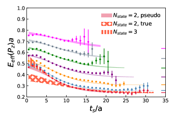
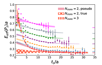
Figure 1: The effective masses obtained from SP (left) and SS (right) correlators for different momenta showed in Eq. (3). The bands come from the results of two-state ($N_{\mathrm{state}}=2$) and three-state ($N_{\mathrm{state}}=3$) fits. For $N_{\mathrm{state}}=2$, ‘pseudo’ indicates that the effective pseudo-plateau in range $5a<t_{\rm min}<10a$ for the first excited state $E_{1}$ have been used, and ‘true’ indicates that the true plateau value of $E_{1}$ in range $t_{\rm min}>11a$ have been used (see text for details).

The effective mass should approach a constant corresponding to the ground state energy $E_{0}(P_{z})$ at sufficiently large $t_{s}$. The momentum dependence of the ground state energy is expected to be described by the dispersion relation $E_{0}(P_{z})=\sqrt{P_{z}^{2}+M^{2}}$, with $M$ being the nucleon mass. Therefore, in Fig. 1, we show the expected ground state energy at different $P_{z}$ obtained from the dispersion relation as horizontal lines at the right for comparison. Along with the expected asymptotic values at large $t_{s}$, we also show the $t_{s}$-dependence of the effective mass based on an effective two-state fit to the two-point function, as we will explain shortly. Indeed, we see that the effective masses approach the corresponding values. The effective masses corresponding to the SP correlator reach a plateau at a slightly larger $t_{s}$ than the SS correlators. On the other hand, at small $t_{s}$, the effective masses for the SP correlators are smaller than those for SS correlators. This implies that the contribution of the excited states is smaller for the SP correlator, for which a plausible reason could be that the different excited states contribute with different signs to the correlator. Thus, even though the ground and the excited state energies are the same in the SP and SS correlators, the two are affected differently by the higher excited states, which we can take advantage of to obtain the excited state spectrum reliably.

In order to determine the energy levels, we fit the spectral decomposition of $C_{\rm 2pt}(t_{s})$,

$$C_{\rm 2pt}(t_{s})=\sum_{n=0}^{N_{\rm state}-1}A_{n}e^{-E_{n}t_{s}},$$ (13)

truncated at $N_{\rm state}$ to the two-point function data over a range of values of $t_{s}$ between $[t_{\rm min},32a]$. Since the lattice extent in the time direction is 192, we did not find any effect of lattice periodicity in this range of $t_{s}$ to be important. We performed this fitting with one-state ($N_{\rm state}=1$), two-state ($N_{\rm state}=2$), and three-state ($N_{\rm state}=3$) Ansätze. The ground state energies, $E_{0}$ from the fits of SS correlators for $n_{z}=3$ and $4$ are shown in left panels of Fig. 2 as function of $t_{\rm min}$, where $t_{\rm min}$ indicates that only $C_{\rm 2pt}(t_{s}>t_{\mathrm{min}})$ have been fitted. Similar results were obtained at the other values of the momenta. The horizontal lines in the figures correspond to the results from the dispersion relation for $E_{0}$. The single exponential fits give a good description of the SS correlator for $t_{\rm min}>11a$, while two exponential fits give stable results for the ground state energy already for $t_{\rm min}>5a$.

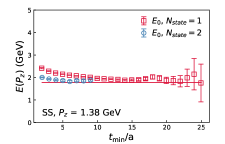
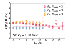
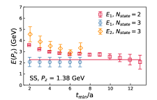
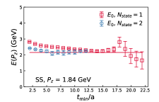
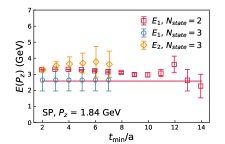
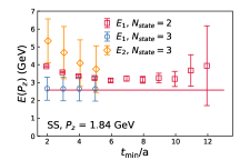
Figure 2: Fit results for $n_{z}=3$ (up) and $n_{z}=4$ (down) the nucleon two-point function. Left panels are for the ground state ($E_{0}$) from one-state and two-state fits. Middle and right panels are for the first ($E_{1}$) and second ($E_{2}$) excited states, determined by two-state and three-state prior-based fits (see text for details). The horizontal lines are the values calculated from the dispersion relation.

We found the determination of the excited state energies from the SS correlators to be more problematic than from SP correlators. The excited state energy for SS is not well-constrained by simple two exponential fits, and it is also not very stable with respect to the variation of $t_{\rm min}$. Since the SP and SS correlators receive different contributions from excited states, we performed a combined analysis of them to obtain more reliable results for the excited state energies. Since we were able to obtain the ground state energy $E_{0}$ reliably from one or two exponential fits to both the SS and SP correlators and they agree with the expectation from the dispersion relation well, we used $E_{0}$ as a prior to performed more stable two-exponential fits. The results from the two-state exponential fits, with $E_{0}$ as prior, for $n_{z}=3$ and $n_{z}=4$ are shown in middle and right panels Fig. 2 for the SP and SS correlators, respectively. For the SP correlators, the excited state energy $E_{1}$ seems to approach a plateau smoothly for $t_{\rm min}>13a$. It is interesting to note that, empirically, we observe the values of the plateaus agree with the dispersion relation $E_{1}(P_{z})=\sqrt{P_{z}^{2}+E_{1}(P_{z}=0)^{2}}$, which are shown as the horizontal lines. While being an interesting observation, such a stringent identification of this state is not important to our analysis and requires further studies to rigorously establish this. For the SS correlator, $E_{1}$ develops a pseudo-plateau for $5a<t_{\rm min}<10a$ and it relaxes to the true plateau (i.e., as identified from the SP case) for $t_{\rm min}>11a$. For $n_{z}=4$, it is actually difficult to identify the true plateau. To model the excited state contributions to $R(\tau,t_{s})$ in the range $0<\tau<t_{s}/2$, with $t_{s}=16a,18a,20a$, one might consider using the well-determined values of $E_{0}$ and $E_{1}$ from the SP correlator at large $t_{s}$. However, as we will demonstrate now, such choices provide a less accurate description of the SS two-point function in the range $5a<t_{s}<10a$. A better description of the excited-state contributions to the $C_{\rm 2pt}(5a<t_{s}<10a)$ can be obtained by using the effective pseudo-plateau value of $E_{1}$ in the range of $5a<t_{\rm min}<10a$.

Since, we observe $E_{1}$ to be well-described by a particle-like dispersion relation for sufficiently large $t_{s}$, we perform three-state fits for both SP and SS correlators by imposing a prior on $E_{1}$ as well, using its best estimate from 2-state fit of SP correlators with the corresponding Jackknife errorsIzubuchi et al. (2019). The results are shown in middle and right panels in Fig. 2. We see that with the prior-based three-state exponential fits, we can obtain stable results for the first excited state energy, $E_{1}(P_{z})$, already for relatively small $t_{\rm min}$ which agrees with the dispersion relation value that we input via the prior. The value of the second excited state is also shown in Fig. 2 and it roughly agrees with the values of $E_{1}$ from the two-exponential fit (with prior only on $E_{0}$) at smaller $t_{\rm min}$. Since the value of $E_{2}$ is quite large, the third exponential probably corresponds to a combination of several excited states. In Fig. 1, we show the 1-$\sigma$ bands for the effective mass corresponding to: (1) Two-state fit that uses values of $E_{0}$ and the true value of $E_{1}$; (2) two-state fit obtained by setting $E_{1}$ to be the effective value in the range from $5a<t_{\rm min}<10a$; (3) three-state fit that we described above. We find that the curves (2) and (3) agree quite well with each other in the range of $5a<t_{s}<10a$ and they extrapolate in the similar fashion to the asymptotic value $E_{0}$. However, the curve (1) fails in capturing the data in the range $5a<t_{s}<10a$. Since for our three-point calculations the source-sink separations were chosen to be $t_{s}=16a,18a,20a$, we must model the effective excited state contributions to the three-point functions in the range $0<\tau<t_{s}/2$. Thus, through this analysis on SP and SS correlators, we numerically demonstrate the usage of an effective value of $E_{1}$ in the range of $5a<t_{s}<10a$ that is higher than the true value of $E_{1}$ is justified, and is the best extrapolation one could perform for the extraction of bare matrix elements in the absence of enough data to perform a three-state fit.

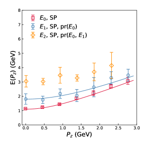
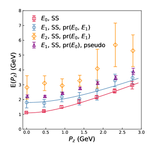
Figure 3: The energies of different states as function of $P_{z}$. On the left panel, the $P_{z}$ dependence of $E_{0}$, $E_{1}$ and $E_{2}$ for SP correlators are shown. The values of $E_{1}$ were obtained from two-state fit with prior only on $E_{0}$, and $E_{2}$ from a three-state fit with priors on both $E_{0}$ and $E_{1}$. On the right panel, the $P_{z}$ dependence of true values (blue points) and effective values of $E_{1}$ (purple points) for SS correlators are both shown (see text for details). The lines indicate the corresponding continuum dispersion relations.

Let us now, summarize the analysis of the nucleon two-point function. Using boosted Gaussian sources we were able to extract ground state energy levels up to momenta $2.7$ GeV from SP and SS correlators. The ground state energy dependence on $P_{z}$ seem to follow the continuum dispersion relation. Using this fact, we performed prior-based fits using the energy from the dispersion relation as a prior and extracted the excited state energies as function of $P_{z}$. For SP correlator the extracted value of $E_{1}$ agrees well with the one from the dispersion relation. We show this in the left panel of Fig. 3. Furthermore, we were able to extract an effective third energy level. These results are shown as blue points ($E_{1}$) and orange points ($E_{2}$) in the left panel of Fig. 3. Our results for the energy levels obtained from SS as function of $P_{z}$ are summarized in right panel of Fig. 3. Here, the effective values of $E_{1}$ from the pseudo-plateau and the true values are both showed. The main point of the elaborate analysis is that even though a third excited state contributes in the relatively shorter range of $t_{s}$ we use in the paper, it possible to describe the SS correlator very well by a two state form with an effective value of $E_{1}$, which is larger than the energy of the physical excited state. Further details on the analysis of the two-point functions are provided in Appendix A.

IV Nucleon three-point correlators

In order to obtain the nucleon qPDF matrix element we consider the ratio of the 3-point function to 2-point function, $R(z,P_{z};t_{s},\tau)$, at different source sink separations, $t_{s}$, and operator insertion, $\tau$. At fixed $(z,P_{z})$ we are interested in fitting the $(t_{s},\tau)$-dependence as expected from the spectral decomposition of $R$. If only two states contribute to the correlation functions, the dependence of this ratio on $\tau$ and $t_{s}$ is given by the following form:

$$R^{\rm fit}_{3}(t_{s},\tau)=\frac{B_{0}+e^{-\Delta Et_{s}/2}\left(B_{1}e^{-\Delta E(t_{s}/2-\tau)}+B_{2}e^{\Delta E(t_{s}/2-\tau)}\right)+B_{3}e^{-\Delta Et_{s}}}{1+\frac{A_{1}}{A_{0}}e^{-\Delta Et_{s}}}.$$ (14)

Here $B_{0}$ is the desired matrix element $h$, and $\Delta E=E_{1}-E_{0}$. Generically, $B_{1}$ and $B_{2}$ are independent fit parameters, except at $z=0$, where $B_{1}=B_{2}$. If we assume that the terms proportional to $A_{1}$ are small, the denominator can be expanded to leading order to obtain a simpler form

$$R^{\rm fit}_{2}(t_{s},\tau)=B_{0}+e^{-\Delta Et_{s}/2}\left(B_{1}e^{-\Delta E(t_{s}/2-\tau)}+B_{2}e^{\Delta E(t_{s}/2-\tau)}\right)+B_{3}e^{-\Delta Et_{s}}.$$ (15)

Finally, if the term proportional to $B_{3}$ is also small compared to other terms, we get an even simpler expression that depends only on three parameters, $B_{0}$, $B_{1}$ and $B_{2}$:

$$R^{\rm fit}_{1}(t_{s},\tau)=B_{0}+e^{-\Delta Et_{s}/2}\left(B_{1}e^{-\Delta E(t_{s}/2-\tau)}+B_{2}e^{\Delta E(t_{s}/2-\tau)}\right).$$ (16)

For each $(z,P_{z})$, we fitted the $(t_{s},\tau)$-dependence of $R(z,P_{z};t_{s},\tau)$ to Eqs. (14, 15, 16) and determined $B_{0}$ in each case. In all these fits we used a fixed value of $\Delta E(P_{z})=E_{1}(P_{z})-E_{0}(P_{z})$, with the pseudo-plateau values of $E_{1}(P_{z})$ and the ground state energies $E_{0}(P_{z})$ determined from the 2-point SS correlation function, as shown in Fig. 3(right).

In the following, we discuss the ratio of the 3-point function to 2-point function, $R(z,P_{z};t_{s},\tau)$, and the corresponding fits for $\Gamma=\gamma_{t}$ and $n_{z}=4$. In Fig. 4, we show the lattice data on this ratio, together with the fit results for two representative values of $z$, namely $z=0$ and $z=8a$. The $t_{s}$ dependence of the lattice results is small compared to the statistical errors. In particular, the difference between $t_{s}=12a$ and $t_{s}=16a$ data is quite small. This means that the contribution of the excited states is not large even though the source-sink separation is below 1 fm. Given that the $t_{s}$-dependence of the ratio is small, it is natural to set $B_{3}=0$ since the term is suppressed by $e^{-t_{s}\Delta E}$, and perform fits using $R^{\rm fit}_{3}(t_{s},\tau)$. We performed fits of the lattice results using the three different fit forms above and the value of $\Delta E$ obtained from two-state fits of the 2-point functions with $t_{\rm min}=6a$. We used operator insertion time $\tau\geqslant\tau_{\rm min}=2a$ in the fits. The matrix elements, $B_{0}$, were obtained using the three fit functions agree within errors. The real and imaginary part of the ratio $R$ should be symmetric and antisymmetric with respect to $z=0$ at any fixed $t_{s}$ and $\tau$. In general, our lattice data is compatible with this expectation. Hence, we symmetrize and antisymmetrize the real and imaginary part of the ratio with respect to $z=0$. The $z$-dependence of the bare matrix elements is shown in Fig. 5 for all three types of fits. We see again that all three fits give the consistent results within errors. Since $B_{0}$ obtained from $R^{\rm fit}_{3}$ and $R^{\rm fit}_{2}$ are consistent with that obtained from $R^{\rm fit}_{1}$, but with larger errors, in the following we will focus on the results obtained from $R^{\rm fit}_{1}$. We also carried out additional checks for any systematic effects, as discussed below.

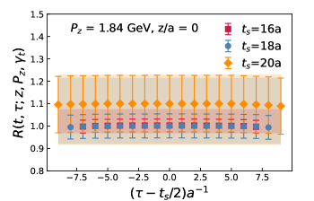
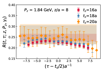
Figure 4: The real part ratio of the three-point function to two-point function at $z=0$ (left) and $z=8a$ (right) as a function of $\tau$ and for different $t_{s}$. The red, orange and gray bands correspond to the bare matrix elements $B_{0}$ extracted from fits to $R^{\rm fit}_{1}$, $R^{\rm fit}_{2}$ and $R^{\rm fit}_{3}$, respectively.

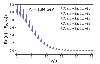
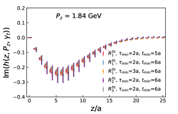
Figure 5: The $z$ dependence of the bare matrix element for $n_{z}=4$. The left panel corresponds to the real part and the right panel corresponds to the imaginary part. The different colors are the matrix elements obtained by various extrapolation methods (denoted by $R_{1}^{\rm fit},R_{2}^{\rm fit}$ and $R_{3}^{\rm fit}$), the number of operator insertion points skipped near source and sink (denoted by $\tau_{\rm min}$), and the $t_{\rm min}$ value in two-point function fit from which the excited state $E_{1}$ was obtained from.

We performed several checks to understand the systematic effects in $R^{\rm fit}_{1}$. First, we studied the dependence of the extracted matrix element on $\tau_{\rm min}$ and found no significant dependence on it. Second, we performed the fits using only a single source-sink separation $t_{s}$ and compared the corresponding results from the three values of $t_{s}$. Interestingly, the matrix elements calculated for source sink separation $t_{s}=16a,~{}18a$ and $20a$ agree within errors, though the $t_{s}=20a$ results have very large errors. We also studied the variation of the extracting matrix element on $\Delta E$ by using $E_{1}$ obtained using different values of $t_{\rm min}$. We found no significant variation. Finally, we used the summation method to obtain the matrix element. This determination has very large statistical errors but it is still compatible with all other determinations. The above checks of systematic effects are discussed further in the Appendix B. We performed a similar analysis for the three-point functions corresponding to the helicity qPDF, i.e. for $\Gamma=\gamma_{z}\gamma_{5}$. Details of those analysis also are discussed in the Appendix B.

V Nonperturbative renormalization

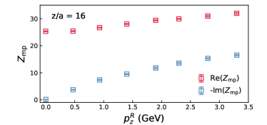
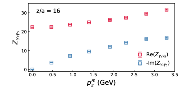
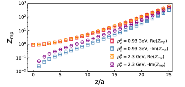
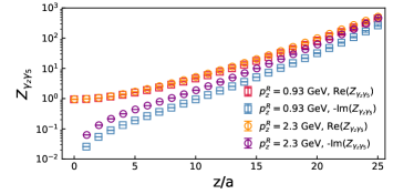
Figure 6: The renormalization constant $Z_{\rm mp}$ and $Z_{\gamma_{z}\gamma_{5}}$ at $\mu_{R}=4~{}$GeV. The upper panels show $Z_{\rm mp}$ and $Z_{\gamma_{z}\gamma_{5}}$ as a function of $p^{R}_{z}$ at $z=16a\approx 0.67$ fm. The lower panels show the $z/a$ dependence with $p_{z}^{R}$ = 0.93 GeV and 2.3 GeV.

We calculate the nonperturbative renormalization of the qPDF operator in the RI-MOM scheme using off-shell quark states in the Landau gauge Alexandrou et al. (2017); Chen et al. (2018a). The matrix element of $O_{\Gamma}(z)$ in an off-shell quark state $|p\rangle$ is

$$\Lambda(p,z,\Gamma)=\langle S(p)\rangle^{-1}\left\langle\sum_{w}{\gamma_{5}}S^{\dagger}(p,w+zn){\gamma_{5}}\Gamma W_{z}(w+zn,w)S(p,w)\right\rangle\langle S(p)\rangle^{-1}\ ,$$ (17)

where $n^{\mu}=(0,0,0,1)$ is the unit vector along the $z$ direction, and the summation is over all lattice sites $w$. The quark propagators are defined as

$$S(p,x)=\sum_{y}e^{ipy}\langle\bar{\psi}(x)\psi(y)\rangle\ ,\ S(p)=\sum_{x}e^{-ipx}S(p,x),$$ (18)

and $\gamma_{5}$ is inserted on both sides of $S^{\dagger}(p,w+zn)$ in Eq. 17 to get the necessary propagator $\sum_{y}e^{-ipy}\langle\bar{\psi}(y)\psi(w+zn)\rangle$.

For the unpolarized qPDF, we use the RI-MOM renormalization constant defined via

$$Z_{\rm mp}(z,p^{R}_{z},a^{-1},\mu_{R})=\left.\frac{\mathrm{Tr}[{\cal P}\Lambda_{\rm tree}(p,z,\gamma_{t})]}{\mathrm{Tr}[{\cal P}\Lambda(p,z,\gamma_{t})]}\right|_{p^{2}=\mu_{R}^{2},\ p_{z}=p^{R}_{z}},$$ (19)

where $\Lambda_{\rm tree}(p,z,\gamma_{t})=\gamma_{t}e^{-izp_{z}}$ is the tree level matrix element in the momentum space. Furthermore, ${\mathcal{P}}=\gamma_{t}-(p_{t}/p_{x})\gamma_{x}$ is the projection operator corresponding to the so-called minimal projection, where only the term with the Dirac structure proportional to $\gamma_{t}$ is kept Stewart and Zhao (2018); Liu et al. (2020). Hence, we use the subscript ‘mp’ for the renormalization constant. The renormalization constant $Z_{\rm mp}(z,p^{R}_{z},a^{-1},\mu_{R})$ depends on the lattice spacing $a$, as well as the other two scales $p^{R}_{z}$ and $\mu_{R}$.

We followed a similar procedure for the longitudinally polarized case, where the RI-MOM renormalization constant is defined as

$$Z_{\gamma_{z}\gamma_{5}}(z,p^{R}_{z},a^{-1},\mu_{R})=\left.\frac{\mathrm{Tr}[{\cal P}\Lambda_{\rm tree}(p,z,\gamma_{z}\gamma_{5})]}{\mathrm{Tr}[{\cal P}\Lambda(p,z,\gamma_{z}\gamma_{5})]}\right|_{p^{2}=\mu_{R}^{2},\ p_{z}=p^{R}_{z}},$$ (20)

with $\Lambda_{tree}(z,p_{z},\gamma_{z}\gamma_{5})=\gamma_{z}\gamma_{5}e^{-ip_{z}z}$. The projection operator ${\cal P}$ in this case was chosen to be ${\cal P}=\gamma_{5}\gamma_{z}/4$.

We calculated the non-perturbative RI-MOM renormalization constants in Landau gauge. The calculations were performed using 14 gauge configurations. The relative uncertainties of the renormalization constants for $z=0,16,32$ are 0.02%, 1% and 10%, respectively. Such precision is much better than that of our nucleon matrix elements with the same $z$, so it is enough at the present stage. We used the following values of the momenta for the off-shell quark state: $ap=\frac{2\pi}{L}(5,5,5,0)$, $\frac{2\pi}{L}(6,2,1,17/3)$ and $\frac{2\pi}{L}(7,4,3,1/3)$, $L=64$ being the spatial size the of the lattice. These momenta correspond to $\mu_{R}=|p|=3.99$ GeV, $3.94$ GeV and $3.97$ GeV, i.e. to $\mu_{R}\sim 4$ GeV within $1.5\%$. Since all the spatial directions are equivalent, each of them could be considered as the $z$-direction and, therefore, with the above choice of the three momenta we have $p_{z}^{R}=0.46\times\{0,1,2,\ldots,7\}$ GeV.

The renormalization constant is plotted in Fig. 6. Due to the linear divergence, the renormalization constant can be far from 1 at a large $z\approx 0.67$ fm, making the nonperturbative renormalization unavoidable. Fig. 6 also shows that the renormalization constant will be sensitive to the value of $p^{R}_{z}$, while such a dependence should be canceled by the matching in the continuum if we have the matching formula up to all orders, because the PDFs or the Mellin moments in $\overline{\rm MS}$ scheme have no dependence on $p^{R}_{z}$. We will consider the residual $p^{R}_{z}$ dependence in the final PDF prediction as a systematic uncertainty.

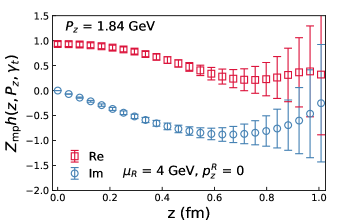
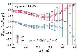
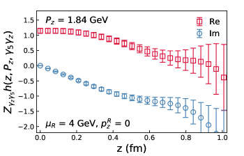
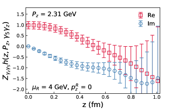
Figure 7: Top panels: The $z$-dependence of the real and imaginary parts of the RI-MOM renormalized (modulo the wavefunction renormalization, $Z_{q}$) unpolarized qPDF matrix element for $P_{z}$ = 1.84 GeV (left) and 2.31 GeV (right). Bottom panels: Similar results for the real and imaginary parts of the helicity matrix element.

Having determined the renormalization constants $Z_{\rm mp}$ and $Z_{\gamma_{z}\gamma_{5}}$ we obtained the renormalized matrix elements, i.e., coordinate space qPDF. For the unpolarized case,

$$h_{R}(z,P_{z},\mu_{R},p_{z}^{R})=Z_{q}Z_{\rm mp}(z,p_{z}^{R},a^{-1},\mu_{R})h(z,P_{z},\gamma_{t}),$$ (21)

and for longitudinally polarized case,

$$\Delta h_{R}(z,P_{z},\mu_{R},p_{z}^{R})=Z_{q}Z_{\gamma_{z}\gamma_{5}}(z,p_{z}^{R},a^{-1},\mu_{R})h(z,P_{z},\gamma_{z}\gamma_{5}).$$ (22)

In the above equations, $Z_{q}$ is the quark wavefunction renormalization factor.

In Fig. 7 we show the renormalized matrix elements, modulo the factor $Z_{q}$, in the RI-MOM scheme at $p_{z}^{R}=0$, $\mu_{R}=4$ GeV. We find that the errors are large. We can achieve substantial error reductions at $z\neq 0$, by redefining the renormalized matrix elements as

$$h_{R}(z,P_{z},\mu_{R},p_{z}^{R})\equiv\frac{h_{R}(z,P_{z},\mu_{R},p_{z}^{R})}{h_{R}(z=0,P_{z},\mu_{R},p_{z}^{R})},\qquad\mathrm{and}\qquad\Delta h_{R}(z,P_{z},\mu_{R},p_{z}^{R})\equiv\frac{\Delta h_{R}(z,P_{z},\mu_{R},p_{z}^{R})}{\Delta h_{R}(z=0,P_{z},\mu_{R},p_{z}^{R})}.$$ (23)

The errors of the matrix elements for $z\neq 0$ are reduced due to the strong correlations between $z\neq 0$ (particularly for for small $z$ close to $z=0$) and $z=0$ matrix elements for each gauge configurations. The effectiveness of this procedure in can be seen from Figs. 12 and 16. As one can see the error reduction due to this division is very significant. In fact, with this method, the errors are reduced enough that the $z$-dependence of the matrix element is well constrained also for $n_{z}=5$. Since for the extraction of the qPDF we are only interested in the $z$-dependence of the matrix element, and we know that the unpolarized isovector nucleon matrix element at $z=0$ is the isospin of the nucleon, which is unity (in our convention, c.f. Eq.  5 ) after renormalization, we can consider the above improved ratio of renormalized matrix elements. However, the effect of taking this ratio is not trivial in the case of the matrix element of the helicity qPDF— the value of the renormalized matrix element at $z=0$ should be $g_{A}\approx 1.3$; this procedure is equivalent to studying a helicity PDF with the first moment normalized to unity, i.e., in a normalization where $g_{A}=1$.

VI Unpolarized PDF: perturbative matching and comparisons with $\mathbf{h_{R}(z,P_{z})}$

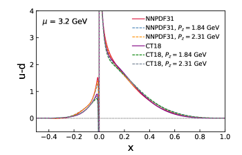
Figure 8: The NNLO isovector nucleon PDFs CT18 Hou et al. (2019) and NNPDF3.1 Ball et al. (2017) (solid lines), and the corresponding target-mass corrected ones (dashed lines), at a scale $\mu=3.2$ GeV. See text for details.

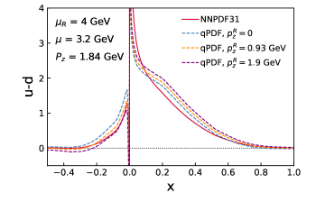
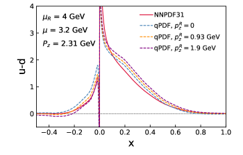
Figure 9: qPDF corresponding to NNPDF3.1 for $P_{z}$=1.84 GeV (left) and $P_{z}$=2.3 GeV (right) with $\alpha_{s}=0.25$ and 3 different RI-MOM renormalization condition.

In this section, we will discuss how the renormalized coordinate-space qPDF, $h_{R}(z,P_{z},\mu_{R},p_{z}^{R})$, can be related and compared with phenomenological unpolarized nucleon PDF, such as the CT18 Hou et al. (2019) and NNPDF3.1 Ball et al. (2017), extracted from the global analysis of experimental data. The unpolarized quark PDF in the valence region is well constrained through global analysis. Therefore, it is natural to start from these phenomenological PDFs as a function of Bjorken-$x$, use the perturbative matching to reconstruct the corresponding coordinate-space qPDF as a function of $z$ for different $P_{z}$ values, and compare with our results for $h_{R}(z,P_{z},\mu_{R},p_{z}^{R})$. The reason for comparing in the $z$-space, rather than constructing the $x$-dependent PDF from our $h_{R}(z,P_{z},\mu_{R},p_{z}^{R})$ and then comparing with the phenomenological PDFs, is the following: As can seen from Figs. 12 and 16, $h_{R}(z,P_{z},\mu_{R},p_{z}^{R})$ is quite noisy for $z\geqslant 0.5$ fm. Thus, the Fourier transformation which is needed to calculate the qPDF in $x$ -space is difficult to perform. Similar approach also had been used for pion PDF Izubuchi et al. (2019).

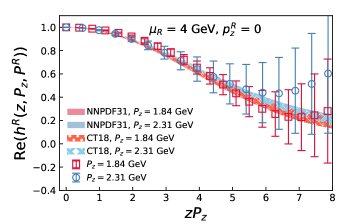
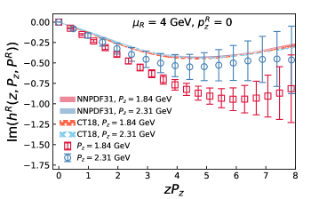
Figure 10: Comparisons of the real (left panel) and imaginary (right panel) parts of the ITDs, in the RI-MOM renormalization at the scales $p_{z}^{R}=0$ and $\mu_{R}=4$ GeV, with that obtained from the CT18 and NNPDF3.1unpolarized isovector nucleon PDFs.

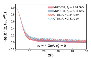
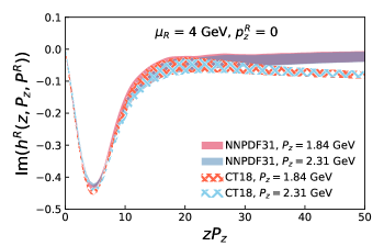
Figure 11: Real (left) and imaginary (right) parts of the ITDs corresponding to target-mass corrected CT18 and NNPDF3.1 PDFs, for $p_{z}^{R}=0$, in an extended range of the Ioffe-time.

Even at the leading $\alpha_{s}^{0}$ order the qPDF and the PDF differ due to the trace term in the small $z$-expansion Ji (2013); Izubuchi et al. (2018). This difference was explicitly calculated in Ref. Chen et al. (2016). In the context of DIS, such corrections have been studied long ago Nachtmann (1973), and are known as target-mass corrections. Following Ref. Chen et al. (2016), we introduce the target-mass corrected PDF

$$q^{\prime}(x,P_{z})=\frac{1}{\sqrt{1+4c}}\left[\frac{f_{+}}{2}q\left(\frac{2x}{f_{+}}\right)-\frac{f_{-}}{2}q\left(\frac{-2x}{f_{-}}\right)\right],$$ (24)

where $c=M^{2}/(4P_{z})^{2}$, $f_{\pm}=\sqrt{1+4c}\pm 1$, $q(x)$ is the usual PDF that corresponds to $P_{z}\rightarrow\infty$. In our analysis we use two sets of NNLO PDF for the u and d quark and anti-quark distributions, the CT18 Hou et al. (2019), and NNPDF3.1 Ball et al. (2017), evaluated at scale $\mu=3.2$ GeV. If the matching was known to all orders of perturbation theory, the prediction for real space qPDF should have been independent of the value of $\mu$ at which the PDF was evaluated. Since the matching only known to 1-loop order, we chose a scale $\mu=3.2$ GeV that is of the same order of the other momentum scales used in our computations and, thereby, avoided corrections due to large logarithms. The lightcone quark PDF for $u$ quark is calculated as $q_{u}(x)=u(x)$, $x>0$ and $q_{u}(x)=-\bar{u}(-x)$, $x<0$. The isovector nucleon PDF, $q_{u}^{\prime}(x)-q_{d}^{\prime}(x)$ is shown in Fig. 8.

In Fig. 8, we also show the target-mass corrected isovector nucleon PDF for the two momenta used in our study, namely 1.84 GeV and 2.31 GeV. We see from the figure that target-mass correction is small for the values of $P_{z}$ used in this study. Using the target-mass corrected NNPDF3.1 isovector nucleon PDF obtained from Eq. (24) and the 1-loop matching to RI-MOM we obtained the corresponding qPDF for $P_{z}=1.84$ GeV and $P_{z}=2.31$ GeV, $\mu_{R}=4$ GeV, and $p_{z}^{R}=0,0.93,1.9$ GeV. The functions $f_{1,\gamma_{t}}$ and $f_{2,\gamma_{t},\mathrm{mp}}$ in Eq. (11) for the 1-loop matching to RI-MOM scheme with minimal projection were taken from Eq. (28) Eq. (31) of Ref. Liu et al. (2020). Fig. 9 shows comparisons of the NNPDF3.1 with the corresponding qPDFs. In these comparisons $\alpha_{s}$ was evaluated at scale $\mu=3.2$ GeV, which resulted in a value $\alpha_{s}=0.25$. We see significant differences between the PDF and qPDF. For large positive $x$, the qPDF is larger than PDF, while for negative $x$ the qPDF can turn negative for some $P_{z}^{R}$. The qPDF strongly depends on the choice of the RI-MOM scales. It is possible to choose the RI-MOM scale such that the qPDF is negative for $x<-0.2$, even though the PDF is positive.

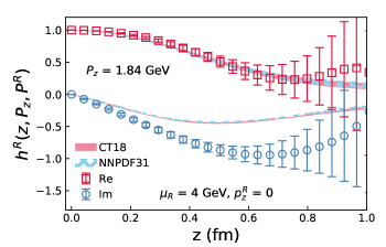
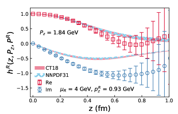
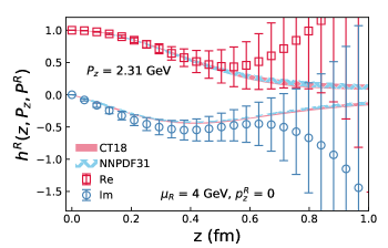
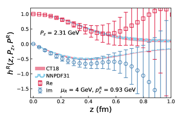
Figure 12: Comparisons of the qPDF with the ones obtained from the global analysis for two values of the RI-MOM renormalization scale, $p_{z}^{R}=0$ GeV (left row) and $p_{z}^{R}=0.93$ GeV (right row), and for two values of the nucleon boost momenta, $P_{z}=1.84$ GeV (upper column) and $P_{z}=2.31$ GeV (lower column).

By Fourier transforming the CT18 and NNPDF3.1 target-mass corrected qPDFs with respect to $x$ we obtained the corresponding distributions as a function of the so-called Ioffe-time, $zP_{z}$, i.e. the corresponding ITDs Ioffe (1969). Since the matching is only up to 1-loop order, the scale entering $\alpha_{s}$ is not fixed. We considered three choices of the scale for $\alpha_{s}$, namely $\mu/2,\mu,2\mu$. The corresponding variations in the ITDs can be considered as estimates of the perturbative uncertainties, and are shown as bands in Fig. 10. In the same figure, also we compare with the lattice results for the ITDs in RI-MOM renormalization, at the renormalization scales of $\mu_{R}=4$ GeV and $p_{z}^{R}=0$ GeV. Albeit large errors, for both values of $P_{z}$ the real parts of the ITDs compare well at least up to $zP_{z}\lesssim 5$. However, lattice results for the imaginary parts of ITDs undershoot the phenomenological ITDs even for $zP_{z}\gtrsim 2$.

Albeit the significant difference between CT18 and NNPDF3.1 PDFs in the small-$x$ region, Fig. 10 do not show any visible difference in their corresponding ITDs. To understand this better, Fig. 11 we explore these ITDs in an extended range of Ioffe-time. The difference between the PDFs in the negative-$x$ region is only reflected in $<10\%$ difference in the imaginary part of the ITDs for $zP_{z}>25$, with essentially showing no difference in the real part ITDs even up to $zP_{z}=50$.

To explore the dependence of the lattice results on the choice of RI-MOM scale $p_{z}^{R}$ and the range of validity of the 1-loop matching, in Fig. 12 we show comparisons between the qPDFs as a function of $z$ obtained in the lattice calculations and from the global analysis of PDF for two different choices of renormalization scale, namely $p_{z}^{R}=0,0.93$ GeV. Very little dependence on the $p_{z}^{R}$ was observed. While the real part of the qPDF obtained from the global analysis agrees with the lattice results up to $z\sim 1$ fm within relative large errors, for the agreement is limited only for $z\lesssim 0.2$ fm. For $P_{z}=2.31$ GeV the agreements seem to extend to larger values of $z$, partly because of larger errors. However, it is encouraging that the central value seems to shift towards the global analysis results as $P_{z}$ is increased from $1.84$ GeV to $2.31$ GeV. In any case, at large $z$, we see clear tension between the imaginary part of the lattice qPDF lattice and the results of global analysis. This suggests that the range of applicability of 1-loop matching is perhaps limited to $z\lesssim 0.2$ fm in the case of the nucleon. It remains to be seen if this agreement gets better with the addition of higher-loop corrections, or this observed discrepancy arises because of contamination of higher-twist effects at larger $z$. This observation has an important implication for our ability to described the $x$-dependence of PDF within the LaMET framework. For example, if the 1-loop perturbative matching works only for $z\simeq 0.2$ fm, reliable calculations of nucleon PDF down to $x\simeq 0.1$ will need $P_{z}\gtrsim 10$ GeV.

VII Helicity PDF: perturbative matching and comparisons with $\mathbf{\Delta h_{R}(z,P_{z})}$

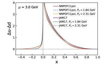
Figure 13: NNPDFpol1.1 and JAM17 isovector helicity PDF at a scale $\mu=3$ GeV. Also, shown are the corresponding target-mass corrected isovector helicity PDFs (dashed lines) for $P_{z}=1.84$ GeV and $P_{z}=2.31$ GeV.

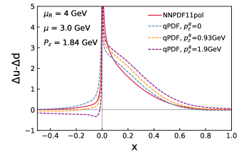
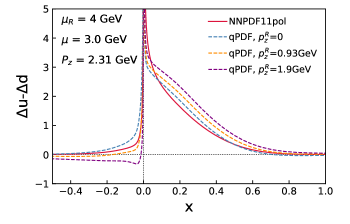
Figure 14: qPDF corresponding to NNPDF1.1pol for $P_{z}$=1.84 GeV (left) and $P_{z}$=2.3 GeV (right) with $\alpha_{s}=0.25$ and 3 different RI-MOM renormalization condition.

Our analysis of helicity qPDF closely follows the analysis performed in the unpolarized case, namely we start from the helicity PDF obtained in global analyses, reconstruct the corresponding target-mass corrected qPDF, and then compare with the lattice results. The helicity PDF have been extracted from the global analysis by NNPDF collaboration using DIS, inclusive $W^{\pm}$ and jet production data from RHIC, as well as the open charm data from COMPAS resulting in NNPDFpol1.1 Nocera et al. (2014). The JAM collaboration used the DIS and SIDIS data in their global analysis, combined with $e^{+}e^{-}$ data to constrain the fragmentation functions at NLO Ethier et al. (2017). The resulting PDF parameterization is called JAM17. In Fig. 13, we show the isovector helicity PDF $\Delta q_{u}-\Delta q_{d}$. The positive-$x$ region corresponds to quark contribution, while the negative-$x$ region corresponds to anti-quark region. The target-mass corrected helicity PDF, $\Delta q^{\prime}(x,P_{z})$, was obtained from helicity PDF, $\Delta q(x)$, following Ref. Chen et al. (2016):

$$\Delta q^{\prime}(x,P_{z})=\frac{1}{1+4c}\left[\frac{f_{+}}{2}\Delta q\left(\frac{2x}{f_{+}}\right)+\frac{f_{-}}{2}\Delta q\left(\frac{-2x}{f_{-}}\right)\right]-\int^{x}_{\pm\infty}\frac{2c}{(1+4c)^{3/2}}\left[\Delta q\left(\frac{2y}{f_{+}}\right)+\Delta q\left(\frac{-2y}{f_{-}}\right)\right],$$ (25)

where $c=M^{2}/4P_{z}^{2}$, $f_{\pm}=\sqrt{1+4c}\pm 1$, and for the integration limits $+\infty$ (-$\infty$) correspond to $x>0$ ($x<0$).

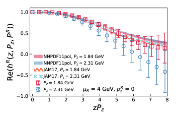
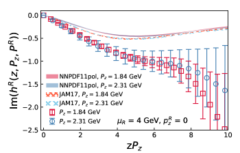
Figure 15: Comparisons of the real (left panel) and imaginary (right panel) parts of the isovector helicity ITDs, in the RI-MOM renormalization at the scales $p_{z}^{R}=0$ and $\mu_{R}=4$ GeV, with that obtained from the NNPDF1.1pol and JAM17.

Although the matching for helicity qPDF has not been explicitly presented in the literature before, it was straightforwardly deduced from the results presented in Ref. Liu et al. (2020). The key observation here was the fact that, owing to the chiral symmetry, for a mass-less quarks in 1-loop perturbation theory $\mathrm{Tr}[\gamma_{5}\gamma_{z}\Lambda(p,z,\gamma_{z}\gamma_{5})]=\mathrm{Tr}[\gamma_{z}\Lambda(p,z,\gamma_{z})]$. Thus, the 1-loop matching of the helicity qPDF in the RI-MOM scheme with minimal projection is same as that for the unpolarized qPDF with $\Gamma=\gamma_{z}$ (instead of the $\Gamma=\gamma_{t}$ used before), and with the RI-MOM renormalization condition corresponding to the projection operator $\mathcal{P}=\gamma_{z}$ (instead of the minimal projection). The 1-loop matching for the $\Gamma=\gamma_{z}$ operator is known for two different RI-MOM projections, the minimal projection and the $\not{p}$ projection, corresponding to $\mathcal{P}=\gamma_{z}-(p_{z}/p_{x})\gamma_{x}$ and $\mathcal{P}=\not{p}/(4p_{z})$, respectively Liu et al. (2020). The function that depends on the RI-MOM projection operator, i.e. $f_{2,\gamma_{z},\gamma_{z}}$, entering the matching coefficient in Eq. 11 was simply deduced from these known results. The Lorentz structure of $\Lambda(p,z,\gamma^{\alpha})$ for a general $\gamma_{\alpha}$, $\alpha=x,y,z,t$ is given by

$$\Lambda^{(1)}(p,x,\gamma_{\alpha})=\gamma_{\alpha}\left[\tilde{f}_{t}(x,\rho)\right]_{+}+\gamma_{z}\frac{p_{\alpha}}{p_{z}}\left[\tilde{f}_{z}(x,\rho)\right]_{+}+\frac{\not{p}p_{\alpha}}{p^{2}}\left[\tilde{f}_{p}(x,\rho)\right]_{+}\,$$ (26)

and $f_{2,\gamma_{z},\mathrm{mp}}=\tilde{f}_{t}+\tilde{f}_{z}$ and $f_{2,\gamma_{z},\not{p}}=\tilde{f}_{t}+\tilde{f}_{z}+\tilde{f}_{p}$ Liu et al. (2020). Here, the subscript ‘+’ refers to the standard plus-prescription and $\rho=-p^{2}/p_{z}^{2}$. The functions $\tilde{f}_{t}$, $\tilde{f}_{z}$ and $\tilde{f}_{p}$ have been calculated in Ref. Liu et al. (2020), and we use the same notations here. Therefore, for the case of $\mathcal{P}=\gamma_{z}$ the RI-MOM projection-dependent function is given by

$$f_{2,\gamma_{z},\gamma_{z}}=\tilde{f}_{t}+\tilde{f}_{z}+(p_{z}^{2}/p^{2})\tilde{f}_{p}=f_{2,\gamma_{z},\mathrm{mp}}+\left(f_{2,\gamma_{z},\not{p}}-f_{2,mp}\right)/r.$$ (27)

Thus, for the helicity qPDF the 1-loop matching RI-MOM function in the minimal projection scheme is the same as in Eq. 11, but with $f_{2,\gamma_{z},\mathrm{mp}}$ given by Eq. 27, and $f_{1,\gamma_{z}}$, $f_{2,\gamma_{z},\mathrm{mp}}$ and $f_{2,\gamma_{z},\not{p}}$ are given by Eqs. (A6-A8) of Ref.  Liu et al. (2020).

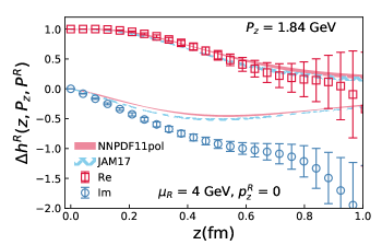
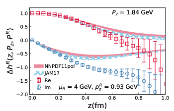
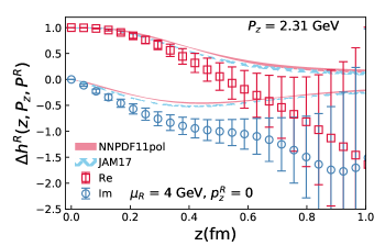
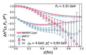
Figure 16: Comparisons of the isovector helicity qPDF with the ones obtained from the global analysis for two values of the RI-MOM renormalization scale, $p_{z}^{R}=0$ GeV (left row) and $p_{z}^{R}=0.93$ GeV (right row), and for two values of the nucleon boost momenta, $P_{z}=1.84$ GeV (upper column) and $P_{z}=2.31$ GeV (lower column).

Using the matching discussed above, we can obtain the isovector helicity qPDF from the target-mass corrected NNPDFpol1.1 and JAM17. As before, the 1-loop matching we used $\alpha_{s}$ evaluated at scale $\mu=3.0$ GeV, and the scale was varied between $\mu/2$ to $2\mu$ to estimate the scale uncertainty. We found noticeable difference between the isovector helicity PDFs and the corresponding qPDFs in Fig. 14. By Fourier transforming the qPDFs we obtained the isovector helicity ITDs and compared it with our lattice results in Fig. 15. Since we normalized our lattice results by the value of matrix element at $z=0$, we normalized the phenomenological ITDs by dividing with $g_{A}=1.25$. Within the large statistical errors, we did not find a significant $P_{z}$ dependence of the lattice results. While the real parts of the lattice results agree with that obtained from the phenomenological PDFs up to $zP_{z}\lesssim 3$, the imaginary parts do not agree quantitatively but also have larger errors. We also explored the dependence of our result on the choice of RI-MOM scales. In Fig. 16, we compare the qPDFs for $\mu_{R}=4$ GeV, and $p_{z}^{R}=0$ GeV and $p_{z}^{R}=0.93$ GeV. From the figure, we see that the comparison between the results of lattice calculation, as well as the global analyses are not sensitive to the choice of the renormalization scales. For both values of $P_{z}$, the agreement between the lattice and the global analyses extends to values of $|z|$ of about $0.3$ fm for the real parts, but not for the imaginary parts. In the next section we will discuss how these disagreements show up in the moments of the PDFs.

VIII Moments of PDF from ratio of Ioffe-time distributions

In the previous sections, we analyzed the boosted nucleon matrix matrix elements renormalized in the RI-MOM scheme and matched it to the PDFs in the $\overline{\rm{MS}}$ scheme. Due to the multiplicative renormalizability of $h(z,P_{z},\gamma_{t})$ and $h(z,P_{z},\gamma_{z}\gamma_{5})$, we can form well-defined renormalized quantities by taking the ratios of matrix elements at two different momenta $P_{z}$ and $P^{\prime}_{z}$ as

$${\cal M}(z,P_{z},P^{\prime}_{z},\Gamma)=\frac{h(z,P_{z},\Gamma)}{h(z,P^{\prime}_{z},\Gamma)}\frac{h(0,P^{\prime}_{z},\Gamma)}{h(0,P_{z},\Gamma)}.$$ (28)

The second factor on the right hand side of the above definition normalizes the $z=0$ matrix element to unity, as we did in the case of the RI-MOM scheme. The choice $P^{\prime}_{z}=0$ in the ratio is usually referred to as the reduced Ioffe-time distributions Radyushkin (2017), and one should think of $P^{\prime}_{z}\neq 0$ as a generalization of this choice. Here, we take $P_{z}=2.31$ GeV and $P^{\prime}_{z}=1.84$ GeV, respectively. Since both $P_{z},P^{\prime}_{z}>\Lambda_{\mathrm{QCD}}$ and the nucleon mass, we expect this ratio to be simply described by the leading twist expression Izubuchi et al. (2018),

$${\cal M}(z,P_{z},P^{\prime}_{z},\Gamma)=\frac{\sum_{n=0}\frac{c_{n}(\mu z)}{c_{0}(\mu z)}\frac{(-izP_{z})^{n}}{n!}\left\langle x^{n}\right\rangle_{P_{z}}(\mu)}{\sum_{n=0}\frac{c_{n}(\mu z)}{c_{0}(\mu z)}\frac{(-izP^{\prime}_{z})^{n}}{n!}\left\langle x^{n}\right\rangle_{P^{\prime}_{z}}(\mu)}.$$ (29)

Following Ref. Chen et al. (2016), the target-mass corrected unpolarized PDF moments $\left\langle x^{n}\right\rangle$ can be obtained by relation:

$$\frac{\left\langle x^{n}\right\rangle_{P_{z}}}{\left\langle x^{n}\right\rangle_{~{}~{}~{}}}=\sum_{i=0}^{\lfloor(n+1)/2\rfloor}C_{n-i+1}^{i}c^{i}$$ (30)

and for the helicity case,

$$\frac{\left\langle x^{n}\right\rangle_{P_{z}}}{\left\langle x^{n}\right\rangle_{~{}~{}~{}}}=\sum_{i=0}^{\lfloor n/2\rfloor}\left(\frac{n-i+1}{n+1}\right)C_{n-i}^{i}c^{i}$$ (31)

where $C_{n}^{i}$ is the binomial function, $c=M^{2}/4P_{z}^{2}$. In Eq. 29, $c_{n}(\mu z)$ is the 1-loop order Wilson coefficients in the $\overline{\mathrm{MS}}$ scheme. The Wilson coefficients describes the $z$ dependence of the twist-2 local operator associated with the $n^{\mathrm{th}}$ moment of the PDF, $\left\langle x^{n}\right\rangle(\mu)$, in the $\overline{\mathrm{MS}}$ scheme and at a factorization scale $\mu$. As in our RI-MOM analysis, we will use $\mu=3.2$ GeV for the unpolarized case and $\mu=3$ GeV for the helicity case in the following analysis.

Now, we can perform an independent analysis that avoids the usage of RI-MOM procedure completely and compare the outcome to the prediction for ${\cal M}(z,P_{z},P^{\prime}_{z},\Gamma)$ from the knowledge of NNPDF and CTEQ PDF moments. We perform such a comparison in Fig. 17. For this, we used the values of $\left\langle x^{n}\right\rangle(\mu)$ up to an order $n=n_{\mathrm{max}}$ for NNPDF31 in Eq. 29, , and the complete result for CT18, to obtain the phenomenological expectation for the ratio ${\cal M}(z,P_{z},P^{\prime}_{z},\gamma_{t})$. The results obtained by using the truncation order $n_{\mathrm{max}}=2,3,4,20$ using the NNPDF31 values for $\left\langle x^{n}\right\rangle$ are shown as different colored bands in Fig. 17. It is clear that inclusion of up to $n_{\mathrm{max}}=20$ moments is sufficient for convergence to the correct PDF within $z\leqslant 0.5$ fm. For $z<0.3$ fm, which is where the lattice data has a good signal to noise ratio, we find that $N=4$ is sufficient to describe the lattice results. This gives us an idea of which moments are being probed by our lattice data at different $z$. We observe some discernible differences between the phenomenological expectations and our lattice ${\cal M}(z,P_{z},P^{\prime}_{z},\gamma_{t})$ for $z>0.2$ fm, as we also observed in the case of RI-MOM scheme in Fig. 10. To understand this, we estimate the values of the moments $\left\langle x^{n}\right\rangle$ that best describe our lattice data. To avoid overfitting the data, we truncate the expansion in Eq. 29 at most by $n=4$. In order to avoid lattice artifacts that might be present for $z$ of the order of lattice spacing, we fit the data only from $z=2a$ to a value $z_{\rm max}$. The variation of the best fit values of $\left\langle x^{n}\right\rangle$ with $z_{\rm max}$ is a source of systematic error. In Fig. 18, we show the $z_{\rm max}$ dependence of our estimates for $\left\langle x^{1}\right\rangle,\left\langle x^{2}\right\rangle,\left\langle x^{3}\right\rangle$ and $\left\langle x^{4}\right\rangle$. From Fig. 17, we note the noisy determination of the imaginary part of ${\cal M}$. As a consequence, we find our estimates of $\left\langle x^{1}\right\rangle$ and $\left\langle x^{3}\right\rangle$ to be noisy as well. On the contrary, we were able to determine $\left\langle x^{2}\right\rangle$ and $\left\langle x^{4}\right\rangle$ reasonably well. In addition to $z_{\rm max}$ dependence, we also studied whether our determination of the moments is affected by the order of truncation used in Eq. 29. We observe no significant variations with truncation. For comparison, the NNPDF and CT18 values of these moments are shown by the horizontal lines. Further, when we fix the values of $\left\langle x^{1}\right\rangle$ and $\left\langle x^{3}\right\rangle$ from NNPDF to reduce the number of fit parameters, we find the estimates for $\left\langle x^{2}\right\rangle$ to be slightly elevated in value and in the direction away from NNPDF,CT18 value. To a small extent, this is seen in $\left\langle x^{4}\right\rangle$ as well. Thus, the observed difference between our lattice result and the NNPDF, CT18 results could be attributed to this tendency for our lattice values of $\left\langle x^{2}\right\rangle,\left\langle x^{4}\right\rangle$ to be slightly higher than the corresponding phenomenological values.

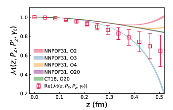
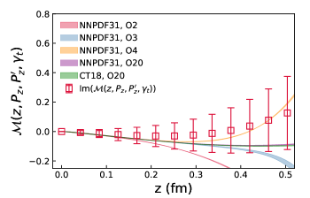
Figure 17: The real (left) and imaginary(right) parts of ${\cal M}(z,P_{z},P^{\prime}_{z},\gamma_{t})$ is shown for $P_{z}=2.31$ GeV and $P^{\prime}_{z}=1.84$ GeV. The data points are from our lattice calculations, whereas the various colored bands are the corresponding results from the isovector unpolarized PDFs from NNPDF3.1 and CT18. The band in these phenomenological expectations arise due to variations of $\alpha_{s}(\mu)$ within the scale scale $\mu/2$ to $2\mu$. For NNPDF3.1, we also show results by truncating the expansion in Eq. 29 at various orders, $n=n_{\mathrm{max}}$, in the PDF moments; these results are denoted by ‘$\mathrm{O}n_{\mathrm{max}}$’.

We repeated similar analysis for the helicity matrix element, $\Gamma=\gamma_{5}\gamma_{z}$. In this case, the Wilson coefficients $c_{n}(\mu z)$ are the same as in the case of unpolarized case with $\Gamma=\gamma_{z}$. Since we are setting the value of the matrix elements at $z=0$ to be 1 through the ratio, we only obtain the values of $\left\langle x^{n}\right\rangle/\left\langle x^{0}\right\rangle$ in the expansion Eq. 29, with $\left\langle x^{0}\right\rangle=g_{A}$. In Fig. 19, we compare the results corresponding to the NNPDF11pol and JAM17 with the lattice result for the ratio. As in the case of the unpolarized matrix element, we also test the dependence of this comparison on the truncation order $n_{\mathrm{max}}$. The sensitivity to higher moments is a bit more than that for the unpolarized case, and we find convergence at only $n_{\mathrm{max}}=6$ at $z<0.3$ fm. Surprisingly, the global fit expectation agrees quite well with our lattice result even though there is a little tension in the imaginary parts. As explained above, we also obtain the best fit values of $\left\langle x^{1}\right\rangle/g_{A},\left\langle x^{2}\right\rangle/g_{A},\left\langle x^{3}\right\rangle/g_{A}$ and $\left\langle x^{4}\right\rangle/g_{A}$ that describe our lattice data via Eq. 29 truncated at most by $4^{\mathrm{th}}$ order. In Fig. 20, we show the results as a function of the largest $z$ used in the fits, $z_{\rm max}$. Like the unpolarized PDF case, $\left\langle x^{1}\right\rangle/g_{A}$ is noisy, but seems agree with the global fit results. The more precisely determined value of $\left\langle x^{2}\right\rangle/g_{A}$ is quite robust to various ways of fitting the data and agrees nicely with the global fit values. To compare with other lattice caculations, we truncate the expansion in Eq. 29 at $n=2$, and estimate $\left\langle x^{1}\right\rangle/g_{A}$ at $\mu$ = 2 GeV with the $z$ in range [2a, 0.3 fm]. Our result $\langle x\rangle/g_{A}$ = 0.219(56) is compatible with the ETMC result Abdel-Rehim et al. (2015) 0.229(30)/1.242(57) within the error.

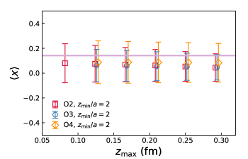
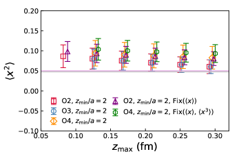
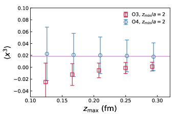
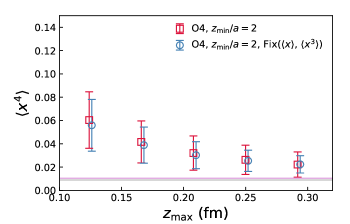
Figure 18: The moments of isovector unpolarized PDF, $\left\langle x^{1}\right\rangle$ (top-left), $\left\langle x^{2}\right\rangle$ (top-right), $\left\langle x^{3}\right\rangle$ (bottom-left), and $\left\langle x^{4}\right\rangle$ (bottom-right), that best describes the ratio ${\cal M}(z,P_{z},P^{\prime}_{z},\gamma_{t})$ with $P_{z}=2.31$ GeV and $P^{\prime}_{z}=1.84$ GeV. In each of the panels, the moment $\left\langle x^{n}\right\rangle$ is shown as a function of $z_{\rm max}$ of the fit using the functional form in Eq. 29 over a range $[2a,z_{\rm max}]$ of the data. The results from fits using only moments up to $n=2$ as free parameters in Eq. 29 are labeled ‘O2’, and those up to $n=4$ are labeled ‘O4’. The results from fits that fix the moment $\left\langle x^{1}\right\rangle$, or $\left\langle x^{1}\right\rangle$ and $\left\langle x^{3}\right\rangle$, to their global fit values are also shown. For comparisons, results from CT18 and NNPDF3.1 are shown as the horizontal lines.

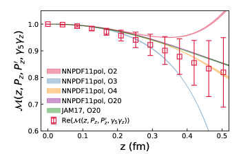
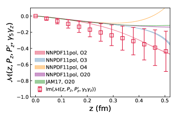
Figure 19: The real (left) and imaginary(right) parts of ${\cal M}(z,P_{z},P^{\prime}_{z},\gamma_{5}\gamma_{z})$ is shown for $P_{z}=2.31$ GeV and $P^{\prime}_{z}=1.84$ GeV. The data points are from our lattice calculations, whereas the various colored bands are the corresponding results from the isovector helicity PDFs from NNPDF1.1pol and JAM17. For NNPDF1.1pol, we also show results by truncating the expansion in Eq. 29 at various orders, $n=n_{\mathrm{max}}$, in the PDF moments; these results are denoted by ‘$\mathrm{O}n_{\mathrm{max}}$’.

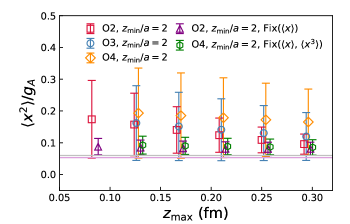
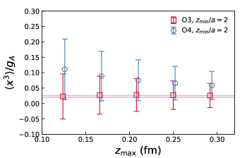
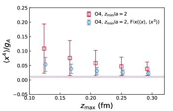
Figure 20: The moments of helicity PDF, $\left\langle x^{1}\right\rangle$ (top-left), $\left\langle x^{2}\right\rangle$ (top-right), $\left\langle x^{3}\right\rangle$ (bottom-left), and $\left\langle x^{4}\right\rangle$ (bottom-right), that best describes the ratio ${\cal M}(z,P_{z},P^{\prime}_{z},\gamma_{5}\gamma_{z})$ with $P_{z}=2.31$ GeV and $P^{\prime}_{z}=1.84$ GeV. In each of the panels, the moment $\left\langle x^{n}\right\rangle$ is shown as a function of $z_{\rm max}$ of the fit using the functional form in Eq. 29 over a range $[2a,z_{\rm max}]$ of the data. The results from fits using only moments up to $n=2$ as free parameters in Eq. 29 are labeled ‘O2’, and those up to $n=4$ are labeled ‘O4’. The results from fits that fix the moment $\left\langle x^{1}\right\rangle$, or $\left\langle x^{1}\right\rangle$ and $\left\langle x^{3}\right\rangle$, to their global fit values are also shown. For comparisons, results from JAM17 and NNPDF1.1pol are shown as the horizontal lines.

IX Summary and conclusions

In this paper we studied isovector unpolarized and helicity PDFs of proton using the LaMET approach. The lattice calculations have been performed for an unphysically large pion mass of $310$ MeV. On the other hand, our lattice study was carried out using lattice spacing $a=0.042$ fm, which is the smallest lattice spacing used in such studies. We argued that such small lattice spacing is essential for the validity of 1-loop perturbative matching between PDF and qPDF, which is a key ingredient of LaMET.

Extracting the nucleon matrix elements for such large momenta and small lattice spacing is challenging because of poor signal to noise ratio. To deal with this problem we performed a detailed study of the nucleon two-point function with momentum smeared source and sink, as well as with momentum smeared source and point sink to better control the excited state contributions. We demonstrated that the ground state can be reliably isolated up to the highest momenta used in this study. Furthermore, for the Euclidean time separations used that are relevant for our lattice analysis the two-point function is very well described by the ground state and and an ’effective’ excited state contribution, with the energy that is larger than the true excited state energy. Therefore, we argued that the two-state Ansätze is sufficient to describe the dependence of the 3-point function on the source-sink separation and on the operator insertion time. We showed that the qPDF matrix elements can be extracted in this way, and the results do no depend on the choices of the fit interval used in our study, demonstrating the robustness of our analysis procedure.

After non-perturbative RI-MOM renormalizations we compared the lattice calculations of the spatial, $z$, dependence of qPDFs with that from the phenomenological PDFs, obtained from the global pQCD-based analyses of pertinent experimental data performed by different collaborations. Working in $z$-space allowed us to test the LaMET approach. The comparisons showed that there is a rough agreement between the lattice results and the results of global analysis, but only at quite small distances. Even for the very small lattice spacing used in this study, there was not enough data points to constrain the $x$-dependence of the PDFs. Instead, to translate our $z$-space comparisons to $x$-dependence, we introduced a new ratio-based renormalization scheme for the Ioffe-time distributions. Using our lattice calculations for Ioffe-time distributions, renormalized via this new ratio-based scheme, we determined the first moments of the isovector unpolarized and helicity PDFs of proton, and compared these moments with that from the corresponding phenomenological PDFs.

Appendix A Analysis of the nucleon two point function

In this appendix we discuss some details of the analysis of the SP and SS two point correlators. In Fig. 21 we show the ground state energy from one and two exponential fits of SP correlators as function of $t_{\rm min}$. Contrary to the fits of the SS correlators stable result for the ground state energy, $E_{0}$ is only obtained for $t_{\rm min}\geq 20$.

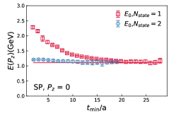
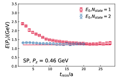
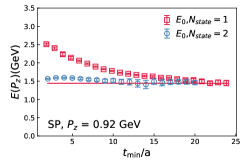
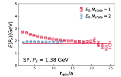
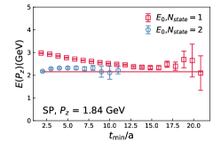
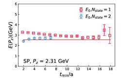
Figure 21: Ground state energy from unconstrained one state fit and two state fit of the SP correlators.

As discussed in the main text we performed prior-based fits of SP and SS correlators for all values of $p_{z}$. In Fig. 22 we show the results on $E_{1}(p_{z})$ for $n_{z}=1,2$ and $5$ for prior-based fits of the SP correlator.

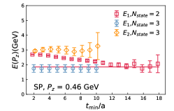
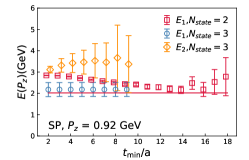
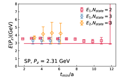
Figure 22: The energies of the first ($E_{1}$) and second ($E_{2}$) excited states from constrained two-state and three-state fits of SP correlator for $n_{z}=1$ (left), $n_{z}=2$ (middle) and $n_{z}=5$ (right). The horizontal line is the values calculated from the dispersion relation.

We see clearly that $E_{1}$ approaches the value expected from the dispersion relation for $t_{\rm min}>11$ if two exponential fit is used. For constrained three exponential fits the same value is approached for $t_{\rm min}=2$. In Fig. 23 we show the amplitudes, $A_{i},~{}i=1,2,3...$, of different states normalized by the value of the two-point correlator at $t=0$, which by definitions is equal to $\sum_{i}A_{i}$. We see that $A_{1}$ is slightly higher than $A_{0}$, while $A_{2}$ is significantly larger than either $A_{0}$ or $A_{1}$.

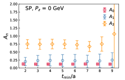
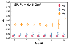
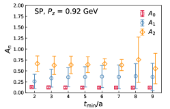
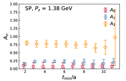
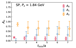
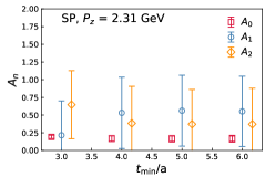
Figure 23: The amplitudes of different states obtained from constrained 3-state fit of SP correlator and normalized by $C_{2pt}^{SP}(t=0)$ as function of temperature.

Similar analysis was performed for SS correlators and the results for the excited state energies and amplitudes are shown in Fig. 24 and Fig. 25, respectively. From these figures we see that a pseudo-plateau develops for the first excited states for $5<t_{\rm min}<10$ of 2-state fit. We see that $A_{0}$ and $A_{1}$ are similar in this case, and $A_{2}$ decreases as $t_{\rm min}$ increasing.

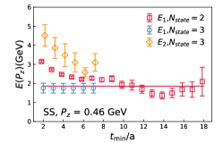
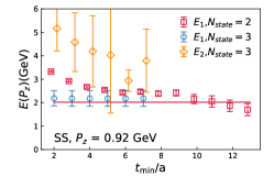
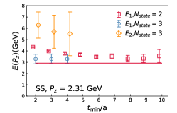
Figure 24: The energies of the first ($E_{1}$) and second ($E_{2}$) excited states from constrained two-state and three-state fits of SS correlator for $n_{z}=1$ (left), $n_{z}=2$ (middle) and $n_{z}=5$ (right). The horizontal line is the values calculated from the dispersion relation.

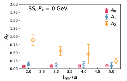
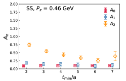
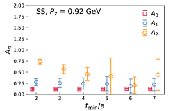
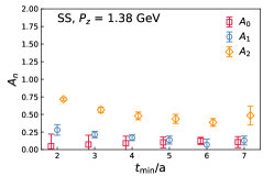
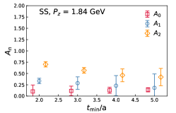
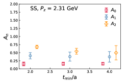
Figure 25: The amplitudes of different states obtained from constrained 3-state fit of SS correlator and normalized by $C_{2pt}^{SS}(t=0)$ as function of temperature.

Appendix B Analysis of the three point function

In this appendix we discuss further details of the extraction of the bare matrix element of the qPDF operator. First, we show our results for the ratio of the 3-point function to two point function for different source sink separation and different values of $z$ as function of the operator insertion time $\tau$ in Fig. 26 for $n_{z}=4$. In this figure we also show the results for $R^{fit}_{1}$. As one can see from the figure $R^{fit}_{1}$ can describe the data well for all values of $t$. In Fig. 27 we show the same analysis but for $n_{z}=5$.

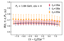
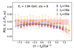
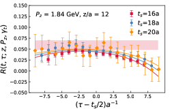
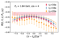
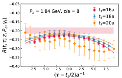
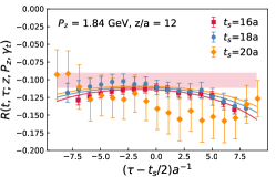
Figure 26: The ratio of the 3-point function to the 2-point function for z=4,8,12 and $n_{z}=4$. The upper panels show the real part, while the imaginary part is shown in the lower panels. The results of $R^{fit}_{1}$ are shown as lines.

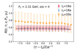
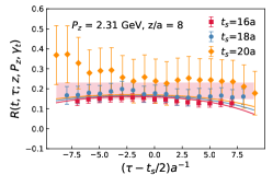
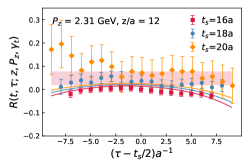
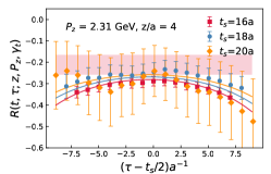
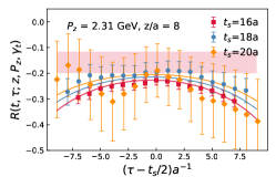
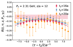
Figure 27: The ratio of the 3-point function to the 2-point function for z=4,8,12 and $n_{z}=5$. The upper panels show the real part, while the imaginary part is shown in the lower panels. The results of $R^{fit}_{1}$ are shown as lines.

As discussed in the main text we performed $R^{fit}_{1}$ using single value of source sink separation. The results are shown in Fig. 28 for the real part of the matrix element. As one can see from the figure the results obtained from this fit for $t=16$, $18$ and $20$ agree within errors. We performed fits using the form $fit_{1}$ with $\tau>\tau_{\rm min}$ and taking the value of $E_{1}$ from the 2-point function fit with $t>t_{\rm min}$. The results are shown in Fig. 29. We see no significant dependence on $\tau_{\rm min}$ and $t_{\rm min}$.

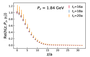
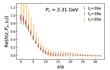
Figure 28: The $z$-dependence of the qPDF matrix element obtained using $R^{fit}_{1}$ with single value of the source sink separation for $n_{z}=4,5$.

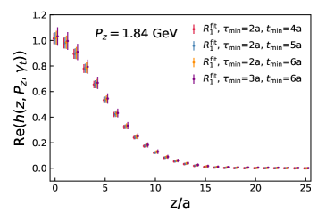
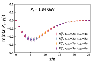
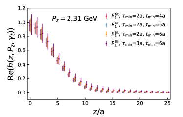
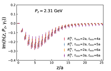
Figure 29: Real (left) and imaginary (right) parts of the bare matrix as function of $z$. The top panel show the result for $n_{z}=4$, the bottom panel show the results for $n_{z}=5$. The results for different choices of $\tau_{\rm min}$ and $t_{\rm min}$ in the 2-point function fits are shown.

Another way to obtain the matrix element is to use the summation method. The summation method is illustrated in Fig. 30 for $n_{z}=4$. The results obtained from the summation method agree with those from $R^{fit}_{1}$ but have much larger errors.

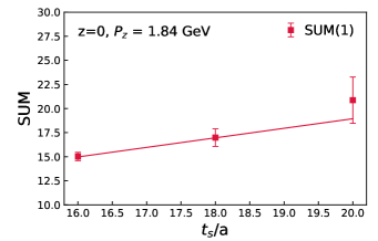
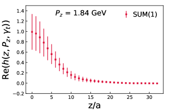
Figure 30: The $t$ dependence of the sum of the ratio of the three point function to two point function (left) and the $z$ dependence of the matrix element extracted from the summation method (right). SUM(n) means summation fit with n skipped time insertion.

The statistical errors of the $n_{z}=5$ data are too large to use the summation method. Furthermore, we could also reduce the error in the summation method by dividing by the matrix element at $z=0$ as can be seen in Fig. 31

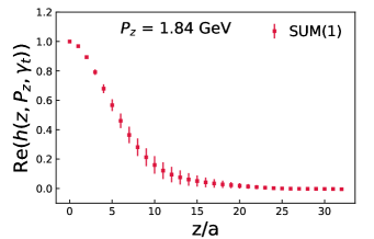
Figure 31: The $z$-dependence of the real part of the bare qPDF matrix element obtained by summation method after division by the matrix element for $z=0$ at $n_{z}=4$. SUM(n) means summation fit with n skipped time insertion.

Similar analysis of the ratio of the three point function to two point function was carries out for longitudinally polarized qPDF operator. The results are summarized in Figs. 32, 33 34.

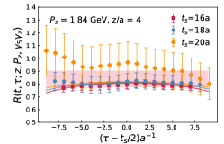
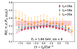
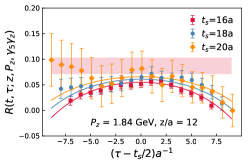
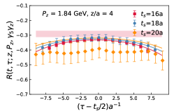
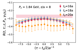
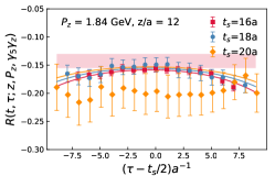
Figure 32: The ratio of the 3-point function to the 2-point function corresponding to helicity qPDF for z=4,8,12 and $n_{z}=4$. The upper panels show the real part, while the imaginary part is shown in the lower panels. The results of $R^{fit}_{1}$ are shown as lines.

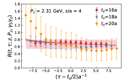
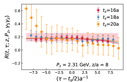
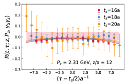
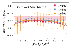
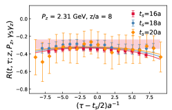
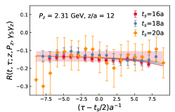
Figure 33: The ratio of the 3-point function to the 2-point function corresponding to helicity qPDF for $z=4,8,12$ and $n_{z}=5$. The upper panels show the real part, while the imaginary part is shown in the lower panels. The results of $R^{fit}_{1}$ are shown as lines.

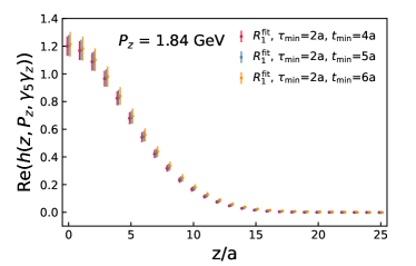
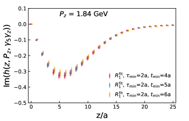
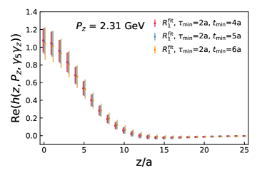
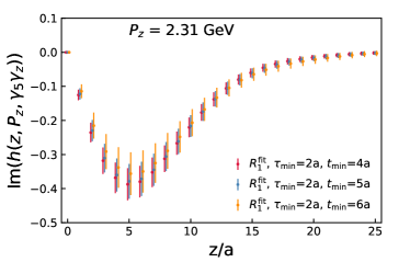
Figure 34: The real (left) and the imaginary (right) parts of the bare matrix corresponding to helicity qPDF. The upper panels correspond to $n_{z}=4$, while the lower panels correspond to $n_{z}=5$. See text for further details.

To take the advantage of correlation between different $z$ and cancel the field renormalization factor, we divided the bare matrix elements by the matrix element at $z=0$. The errors are much smaller after this division as discussed in the main text.

References

- de Florian et al. (2014) D. de Florian, R. Sassot, M. Stratmann, and W. Vogelsang, Phys. Rev. Lett. 113, 012001 (2014), arXiv:1404.4293 [hep-ph] .
- Adamczyk et al. (2015) L. Adamczyk et al. (STAR), Phys. Rev. Lett. 115, 092002 (2015), arXiv:1405.5134 [hep-ex] .
- Adare et al. (2014) A. Adare et al. (PHENIX), Phys. Rev. D90, 012007 (2014), arXiv:1402.6296 [hep-ex] .
- Adare et al. (2016a) A. Adare et al. (PHENIX), Phys. Rev. D93, 011501 (2016a), arXiv:1510.02317 [hep-ex] .
- Adolph et al. (2013) C. Adolph et al. (COMPASS), Phys. Rev. D87, 052018 (2013), arXiv:1211.6849 [hep-ex] .
- Adamczyk et al. (2014) L. Adamczyk et al. (STAR), Phys. Rev. Lett. 113, 072301 (2014), arXiv:1404.6880 [nucl-ex] .
- Adare et al. (2016b) A. Adare et al. (PHENIX), Phys. Rev. D93, 051103 (2016b), arXiv:1504.07451 [hep-ex] .
- Dudek et al. (2012) J. Dudek et al., Eur. Phys. J. A48, 187 (2012), arXiv:1208.1244 [hep-ex] .
- Accardi et al. (2016) A. Accardi et al., Eur. Phys. J. A52, 268 (2016), arXiv:1212.1701 [nucl-ex] .
- Chatrchyan et al. (2012) S. Chatrchyan et al. (CMS), Science 338, 1569 (2012).
- Aad et al. (2012) G. Aad et al. (ATLAS), Science 338, 1576 (2012).
- Ji (2013) X. Ji, Phys. Rev. Lett. 110, 262002 (2013), arXiv:1305.1539 [hep-ph] .
- Ji (2014) X. Ji, Sci. China Phys. Mech. Astron. 57, 1407 (2014), arXiv:1404.6680 [hep-ph] .
- Ma and Qiu (2018a) Y.-Q. Ma and J.-W. Qiu, Phys. Rev. D98, 074021 (2018a), arXiv:1404.6860 [hep-ph] .
- Ma and Qiu (2018b) Y.-Q. Ma and J.-W. Qiu, Phys. Rev. Lett. 120, 022003 (2018b), arXiv:1709.03018 [hep-ph] .
- Radyushkin (2017) A. V. Radyushkin, Phys. Rev. D96, 034025 (2017), arXiv:1705.01488 [hep-ph] .
- Orginos et al. (2017) K. Orginos, A. Radyushkin, J. Karpie, and S. Zafeiropoulos, Phys. Rev. D96, 094503 (2017), arXiv:1706.05373 [hep-ph] .
- Ji et al. (2018) X. Ji, J.-H. Zhang, and Y. Zhao, Phys. Rev. Lett. 120, 112001 (2018), arXiv:1706.08962 [hep-ph] .
- Ishikawa et al. (2017) T. Ishikawa, Y.-Q. Ma, J.-W. Qiu, and S. Yoshida, Phys. Rev. D96, 094019 (2017), arXiv:1707.03107 [hep-ph] .
- Chen et al. (2018a) J.-W. Chen, T. Ishikawa, L. Jin, H.-W. Lin, Y.-B. Yang, J.-H. Zhang, and Y. Zhao, Phys. Rev. D97, 014505 (2018a), arXiv:1706.01295 [hep-lat] .
- Constantinou and Panagopoulos (2017) M. Constantinou and H. Panagopoulos, Phys. Rev. D96, 054506 (2017), arXiv:1705.11193 [hep-lat] .
- Alexandrou et al. (2017) C. Alexandrou, K. Cichy, M. Constantinou, K. Hadjiyiannakou, K. Jansen, H. Panagopoulos, and F. Steffens, Nucl. Phys. B923, 394 (2017), arXiv:1706.00265 [hep-lat] .
- Stewart and Zhao (2018) I. W. Stewart and Y. Zhao, Phys. Rev. D97, 054512 (2018), arXiv:1709.04933 [hep-ph] .
- Liu et al. (2020) Y.-S. Liu et al. (Lattice Parton), Phys. Rev. D 101, 034020 (2020), arXiv:1807.06566 [hep-lat] .
- Izubuchi et al. (2018) T. Izubuchi, X. Ji, L. Jin, I. W. Stewart, and Y. Zhao, Phys. Rev. D98, 056004 (2018), arXiv:1801.03917 [hep-ph] .
- Liu et al. (2018) Y.-S. Liu, J.-W. Chen, L. Jin, R. Li, H.-W. Lin, Y.-B. Yang, J.-H. Zhang, and Y. Zhao, (2018), arXiv:1810.05043 [hep-lat] .
- Lin et al. (2018) H.-W. Lin, J.-W. Chen, X. Ji, L. Jin, R. Li, Y.-S. Liu, Y.-B. Yang, J.-H. Zhang, and Y. Zhao, Phys. Rev. Lett. 121, 242003 (2018), arXiv:1807.07431 [hep-lat] .
- Chen et al. (2018b) J.-W. Chen, L. Jin, H.-W. Lin, Y.-S. Liu, Y.-B. Yang, J.-H. Zhang, and Y. Zhao, (2018b), arXiv:1803.04393 [hep-lat] .
- Alexandrou et al. (2019) C. Alexandrou, K. Cichy, M. Constantinou, K. Hadjiyiannakou, K. Jansen, A. Scapellato, and F. Steffens, Phys. Rev. D99, 114504 (2019), arXiv:1902.00587 [hep-lat] .
- Alexandrou et al. (2018a) C. Alexandrou, K. Cichy, M. Constantinou, K. Jansen, A. Scapellato, and F. Steffens, Phys. Rev. D98, 091503 (2018a), arXiv:1807.00232 [hep-lat] .
- Alexandrou et al. (2018b) C. Alexandrou, K. Cichy, M. Constantinou, K. Jansen, A. Scapellato, and F. Steffens, Phys. Rev. Lett. 121, 112001 (2018b), arXiv:1803.02685 [hep-lat] .
- Joó et al. (2019a) B. Joó, J. Karpie, K. Orginos, A. Radyushkin, D. Richards, and S. Zafeiropoulos, JHEP 12, 081 (2019a), arXiv:1908.09771 [hep-lat] .
- Joó et al. (2020) B. Joó, J. Karpie, K. Orginos, A. V. Radyushkin, D. G. Richards, and S. Zafeiropoulos, (2020), arXiv:2004.01687 [hep-lat] .
- Zhang et al. (2019a) J.-H. Zhang, J.-W. Chen, L. Jin, H.-W. Lin, A. Schär, and Y. Zhao, Phys. Rev. D100, 034505 (2019a), arXiv:1804.01483 [hep-lat] .
- Izubuchi et al. (2019) T. Izubuchi, L. Jin, C. Kallidonis, N. Karthik, S. Mukherjee, P. Petreczky, C. Shugert, and S. Syritsyn, Phys. Rev. D100, 034516 (2019), arXiv:1905.06349 [hep-lat] .
- Sufian et al. (2019) R. S. Sufian, J. Karpie, C. Egerer, K. Orginos, J.-W. Qiu, and D. G. Richards, Phys. Rev. D99, 074507 (2019), arXiv:1901.03921 [hep-lat] .
- Joó et al. (2019b) B. Joó, J. Karpie, K. Orginos, A. V. Radyushkin, D. G. Richards, R. S. Sufian, and S. Zafeiropoulos, Phys. Rev. D100, 114512 (2019b), arXiv:1909.08517 [hep-lat] .
- Sufian et al. (2020) R. S. Sufian, C. Egerer, J. Karpie, R. G. Edwards, Joóánt, Y.-Q. Ma, K. Orginos, J.-W. Qiu, and D. G. Richards, (2020), arXiv:2001.04960 [hep-lat] .
- Zhao (2019) Y. Zhao, Int. J. Mod. Phys. A33, 1830033 (2019), arXiv:1812.07192 [hep-ph] .
- Cichy and Constantinou (2019) K. Cichy and M. Constantinou, Adv. High Energy Phys. 2019, 3036904 (2019), arXiv:1811.07248 [hep-lat] .
- Monahan (2018) C. Monahan, Proceedings, 36th International Symposium on Lattice Field Theory (Lattice 2018): East Lansing, MI, United States, July 22-28, 2018, PoS LATTICE2018, 018 (2018), arXiv:1811.00678 [hep-lat] .
- Ji et al. (2020) X. Ji, Y.-S. Liu, Y. Liu, J.-H. Zhang, and Y. Zhao, (2020), arXiv:2004.03543 [hep-ph] .
- Follana et al. (2007) E. Follana, Q. Mason, C. Davies, K. Hornbostel, G. P. Lepage, J. Shigemitsu, H. Trottier, and K. Wong (HPQCD, UKQCD), Phys. Rev. D75, 054502 (2007), arXiv:hep-lat/0610092 [hep-lat] .
- Bazavov et al. (2013) A. Bazavov et al. (MILC), Phys. Rev. D87, 054505 (2013), arXiv:1212.4768 [hep-lat] .
- Hasenfratz and Knechtli (2001) A. Hasenfratz and F. Knechtli, Phys. Rev. D64, 034504 (2001), arXiv:hep-lat/0103029 [hep-lat] .
- Gupta et al. (2017) R. Gupta, Y.-C. Jang, H.-W. Lin, B. Yoon, and T. Bhattacharya, Phys. Rev. D96, 114503 (2017), arXiv:1705.06834 [hep-lat] .
- Bhattacharya et al. (2015a) T. Bhattacharya, V. Cirigliano, S. Cohen, R. Gupta, A. Joseph, H.-W. Lin, and B. Yoon (PNDME), Phys. Rev. D92, 094511 (2015a), arXiv:1506.06411 [hep-lat] .
- Bhattacharya et al. (2015b) T. Bhattacharya, V. Cirigliano, R. Gupta, H.-W. Lin, and B. Yoon, Phys. Rev. Lett. 115, 212002 (2015b), arXiv:1506.04196 [hep-lat] .
- Bhattacharya et al. (2014) T. Bhattacharya, S. D. Cohen, R. Gupta, A. Joseph, H.-W. Lin, and B. Yoon, Phys. Rev. D89, 094502 (2014), arXiv:1306.5435 [hep-lat] .
- Babich et al. (2010) R. Babich, J. Brannick, R. C. Brower, M. A. Clark, T. A. Manteuffel, S. F. McCormick, J. C. Osborn, and C. Rebbi, Phys. Rev. Lett. 105, 201602 (2010), arXiv:1005.3043 [hep-lat] .
- Osborn et al. (2010) J. C. Osborn, R. Babich, J. Brannick, R. C. Brower, M. A. Clark, S. D. Cohen, and C. Rebbi, Proceedings, 28th International Symposium on Lattice field theory (Lattice 2010): Villasimius, Italy, June 14-19, 2010, PoS LATTICE2010, 037 (2010), arXiv:1011.2775 [hep-lat] .
- Edwards and Joo (2005) R. G. Edwards and B. Joo (SciDAC, LHPC, UKQCD), Lattice field theory. Proceedings, 22nd International Symposium, Lattice 2004, Batavia, USA, June 21-26, 2004, Nucl. Phys. Proc. Suppl. 140, 832 (2005), [,832(2004)], arXiv:hep-lat/0409003 [hep-lat] .
- Bali et al. (2016) G. S. Bali, B. Lang, B. U. Musch, and A. Schaefer, Phys. Rev. D93, 094515 (2016), arXiv:1602.05525 [hep-lat] .
- Chen et al. (2017) J.-W. Chen, T. Ishikawa, L. Jin, H.-W. Lin, Y.-B. Yang, J.-H. Zhang, and Y. Zhao, (2017), arXiv:1710.01089 [hep-lat] .
- Wang et al. (2019) W. Wang, J.-H. Zhang, S. Zhao, and R. Zhu, Phys. Rev. D100, 074509 (2019), arXiv:1904.00978 [hep-ph] .
- Zhang et al. (2019b) J.-H. Zhang, X. Ji, A. Schär, W. Wang, and S. Zhao, Phys. Rev. Lett. 122, 142001 (2019b), arXiv:1808.10824 [hep-ph] .
- Hou et al. (2019) T.-J. Hou et al., (2019), arXiv:1912.10053 [hep-ph] .
- Ball et al. (2017) R. D. Ball et al. (NNPDF), Eur. Phys. J. C77, 663 (2017), arXiv:1706.00428 [hep-ph] .
- Chen et al. (2016) J.-W. Chen, S. D. Cohen, X. Ji, H.-W. Lin, and J.-H. Zhang, Nucl. Phys. B911, 246 (2016), arXiv:1603.06664 [hep-ph] .
- Nachtmann (1973) O. Nachtmann, Nucl. Phys. B63, 237 (1973).
- Ioffe (1969) B. L. Ioffe, Phys. Lett. 30B, 123 (1969).
- Nocera et al. (2014) E. R. Nocera, R. D. Ball, S. Forte, G. Ridolfi, and J. Rojo (NNPDF), Nucl. Phys. B887, 276 (2014), arXiv:1406.5539 [hep-ph] .
- Ethier et al. (2017) J. J. Ethier, N. Sato, and W. Melnitchouk, Phys. Rev. Lett. 119, 132001 (2017), arXiv:1705.05889 [hep-ph] .
- Abdel-Rehim et al. (2015) A. Abdel-Rehim et al., Phys. Rev. D 92, 114513 (2015), [Erratum: Phys.Rev.D 93, 039904 (2016)], arXiv:1507.04936 [hep-lat] .