Visible stripe phases in spin-orbital-angular-
momentum coupled Bose-Einstein condensates

Abstract

Recently, stripe phases in spin-orbit coupled Bose-Einstein condensates (BECs) have attracted much attention since they are identified as supersolid phases. In this paper, we exploit experimentally reachable parameters and show theoretically that annular stripe phases with large stripe spacing and high stripe contrast can be achieved in spin-orbital-angular-momentum coupled (SOAMC) BECs. In addition to using Gross-Pitaevskii numerical simulations, we develop a variational ansatz that captures the essential interaction effects to first order, which are not present in the ansatz employed in previous literature. Our work should open the possibility toward directly observing stripe phases in SOAMC BECs in experiments.

I Introduction

The realization of synthetic gauge fields and spin-orbit coupling (SOC) for ultracold atoms has opened new opportunities for creating and investigating topological matters in a clean and easy-to-manipulate environment Dalibard et al. (2011); Galitski and Spielman (2013); Goldman et al. (2014); Zhai (2015). In the SOC Bose-Einstein condensates (BEC) realized in early works Lin et al. (2011); Wu et al. (2016); Huang et al. (2016), the internal spin states are coupled to the center-of-mass linear momentum of the atoms via Raman laser dressing. There, the Raman beams transfer photon momentum to the atoms as the spin state changes. By using a similar method with Laguerre-Gaussian (LG) Raman beams which transfer orbital-angular-momentum (OAM) between atomic spin states, physicists recently demonstrated a coupling between internal spin states and the center-of-mass OAM Chen et al. (2018a, b); Zhang et al. (2019). In the following, we refer to the former as spin-linear-momentum coupling (SLMC) and the latter as spin-orbital-angular-momentum coupling (SOAMC) .

The interplay between interactions and SLMC leads to interesting quantum phases Wang et al. (2010); Ho and Zhang (2011); Yip (2011); Li et al. (2012); Martone et al. (2014). For a pseudospin $1/2$ system, by tuning the Raman coupling strength from large to small values, the energy-versus-momentum dispersion transforms from a single minimum to double minima (see Fig. 1b). For the latter case, whether the atoms occupy one of the minima or both minima is determined by a competition between inter- and intra-species interactions, where the two species refer to atoms which occupy the two respective minima. When the atoms occupy both minima associated with different quasimomentum, the interference results in density modulations in the position space, which is known as a stripe phase. When only one of the minima is occupied, it is the separated phase, i.e., the plane-wave phase. The stripe phase in SLMC BECs is intriguing since it spontaneously breaks the translational symmetry (being a solid) and the $U(1)$ gauge symmetry (being a superfluid) simultaneously, leading to a so-called supersolid Boninsegni and Prokof’Ev (2012). Analogously, the ground state of SOAMC BECs also has an annular stripe phase and separated phases, which are theoretically studied in Refs. Qu et al. (2015); Sun et al. (2015); DeMarco and Pu (2015); Chen et al. (2016). The annular stripe phase of SOAMC BECs corresponds to occupying both energy minima with different quasiangular-momentum. The stripe spatial period is then $\approx 2\pi R/\Delta\ell$, where $R$ is a typical length scale smaller than the BEC size $R_{\rm BEC}$, and $\Delta\ell$ is the transferred OAM between spin states in units of $\hbar$. Since $R$ is the order of micrometers, the spatial period can be made larger than that in SLMC, which is $\lambda/2$ with $\lambda$ being the optical wavelength of the Raman laser. The submicron stripe period of SLMC BECs is difficult to resolve even with the state-of-the-art quantum gas microscope Bakr et al. (2009).

Due to both the small spatial period and small contrast resulting from small miscibility, direct observations of stripe phases in position space remain elusive to date. Recently, detecting the stripe density modulation using Bragg spectroscopy are demonstrated in spin-linear-momentum-coupled BECs Putra et al. (2020); Li et al. (2017). In the experiment with Raman-coupled internal spin states Putra et al. (2020), the spatial phase coherence of both the stripe and separated phase is demonstrated interferometrically. In Ref. Li et al. (2017), atoms localized within each side of a double well serve as two pseudospin states. This circumvents the problem of detuning noises owing to the magnetic field noises for internal spin states, and enhances the miscibility. The observed stripe contrast is $\sim~{}8~{}\%$ limited by heatings from the Raman driving fields which create SLMC.

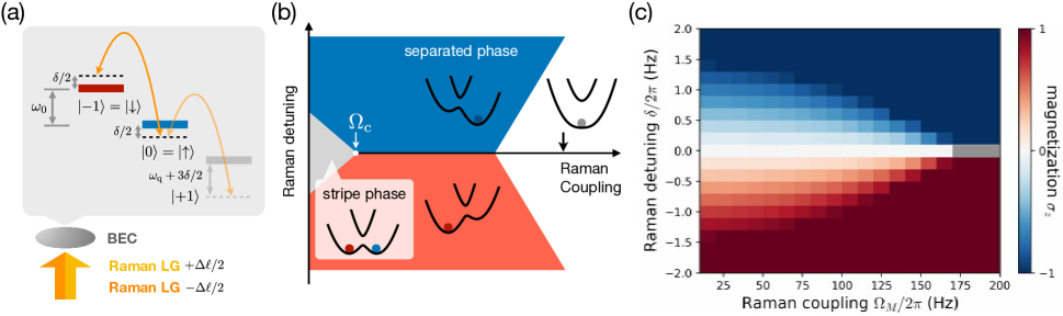
Figure 1: (a) Schematic figure of the $F=1$ SOAMC BEC with the level diagram. The effective two-level scheme can be realized by using a large quadratic Zeeman energy $\omega_{q}$ such that $\left\lvert m_{F}=1\right\rangle$ is off-resonance. (b) Schematic SLMC phase diagram (c) SOAMC phase diagram of atoms in a harmoinc trap. $\Delta\ell=20,r_{M}=5{\ \mu{\rm m}},R_{\rm TF}=12.5{\ \mu{\rm m}}$, and $\mu/h=926$ Hz. For $\delta=0$, the ground state is the stripe (separated) phase with $\Omega_{M}<(>)\Omega_{c}$. For small nonzero detuning, the critical coupling is smaller than the $\Omega_{c}(\delta=0)$ and decreases with increasing $|\delta|$. Near $\Omega_{M}=0$, the stripe phase exists for $|\delta|/2\pi\lesssim 1$ Hz. At $\delta=0$, the magnetization $\sigma_{z}=N_{\uparrow}-N_{\downarrow}$ is zero; the stripe contrast at $\delta=0$ is larger than that at any other nonzero $\delta$. The grey bar at $\delta=0$ and $\Omega_{M}>\Omega_{c}$ indicates the separated phase can have either $\sigma_{z}=1$ or $-1$.

In this paper, we exploit the advantages of SOAMC systems and demonstrate the feasibility to directly observe annular stripe phases in situ with practical experimental parameters. We observe that interactions reduce the stripe density contrast. Here the interaction strength is $\varepsilon_{\rm int}/E_{L}<1$, where $\varepsilon_{\rm int}$ is the mean field interaction energy and $E_{L}=\hbar^{2}\Delta\ell^{2}/2mR^{2}$ is the characteristic energy scale of SOAMC systems. The effects of interactions discussed in previous papers Li et al. (2012); Sun et al. (2015); Chen et al. (2016, 2019) are based on the wave function ansatz that is not fully self-consistent in the presence of interaction. Even within first order in interaction strength, we find that the results of Refs. Li et al. (2012); Sun et al. (2015); Chen et al. (2016, 2019) are subject to significant corrections. We use an improved ansatz and obtain results that are correct to first order in interaction. While in SLMC systems, the analogous interaction strength is $\varepsilon_{\rm int}/4E_{r}$ and is typically small, where the photon recoil energy $E_{r}$ is larger than $E_{L}$. We investigate how the stripe density contrast depends on experimentally accessible parameters: the transferred angular momentum $\Delta\ell$, the size of the OAM-carrying LG Raman beam, the BEC cloud size, and the mean field energy. By optimizing these parameters, we achieve a stripe period of $\sim 2{\ \mu{\rm m}}$ at most and a $\lesssim 30~{}\%$ contrast of density modulations. This is detectable using high-resolution imaging with about $1{\ \mu{\rm m}}$ resolutions Bakr et al. (2009) . Further, the contrast can be made larger than $30~{}\%$ by increasing the BEC cloud size. Finally, we point out that by using synthetic clock states Trypogeorgos et al. (2018), the stripe phase of the thermodynamic ground state can be stable against external magnetic field noises despite the narrow detuning window within which the stripe phase exits.

II Formalism

We consider pseudospin $1/2$ atoms tightly confined along $z$ in a quasi-2D geometry, where $\hbar\omega_{z}>\mu$ with $\omega_{z}$ being the trap frequency along $z$ and $\mu$ the chemical potential. Two Raman beams couple the two spin states with a transfer of orbital-angular-momentum (OAM) $\Delta\ell$ in unit of $\hbar$, and the frequency difference between the two beams is $\Delta\omega_{L}$. In the rotating frame at frequency $\Delta\omega_{L}$ with rotating wave approximation, the single-particle Hamiltonian is

$$\hat{H}_{0}= \left[\frac{-\hbar^{2}}{2m}\frac{\partial}{r\partial r}(r\frac{\partial}{\partial r})+\frac{L_{z}^{2}}{2mr^{2}}+V(r)\right]\otimes{\hat{1}}$$ (1)

$$+\frac{\hbar\delta}{2}\hat{\sigma}_{z}+\frac{\hbar\Omega(r)}{2}\left[\cos(\Delta\ell\phi)\hat{\sigma}_{x}-\sin(\Delta\ell\phi)\hat{\sigma}_{y}\right],$$

where $L_{z}=-i\hbar\partial_{\phi}$ is the angular momentum operator, $V(r)$ is the spin-independent trapping potential, $\delta=\Delta\omega_{L}-\omega_{0}$ is the Raman detuning, and $\hbar\omega_{0}=E_{\downarrow}-E_{\uparrow}$ is the energy splitting between $\left\lvert\downarrow\right\rangle$ and $\left\lvert\uparrow\right\rangle$. The Raman beams are two Laguerre-Gaussian beams of order $\Delta\ell/2$ and $-\Delta\ell/2$, and the coupling strength is

$$\Omega(r)=e^{\Delta\ell/2}\Omega_{M}\left(\frac{r}{r_{M}}\right)^{\Delta\ell}\exp\left[-\frac{\Delta\ell}{2}\frac{r^{2}}{r_{M}^{2}}\right],$$ (2)

where the peak coupling $\Omega_{M}$ is at $r=r_{M}$, and the waist of each beam is $w=2r_{M}/\sqrt{\Delta\ell}$.

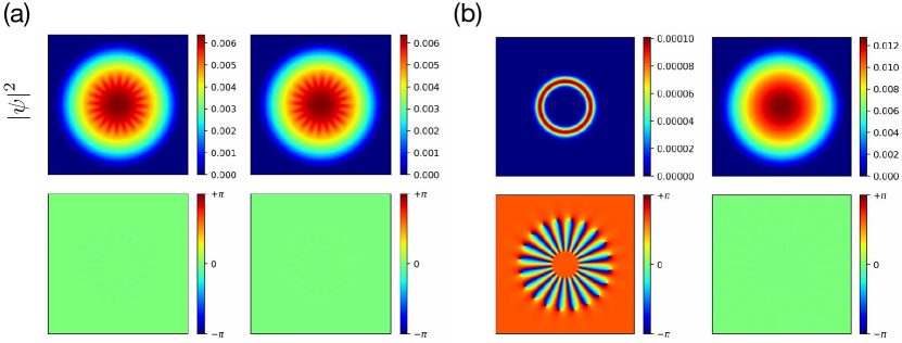
Figure 2: Images of the stripe phase at $\Omega_{M}/2\pi=150$ Hz $<\Omega_{c}$ in (a), and the separated phase at $\Omega_{M}/2\pi=200$ Hz $>\Omega_{c}$ in (b); left (right) panels indicate $\left\lvert\uparrow\right\rangle(\left\lvert\downarrow\right\rangle)$, and top (bottom) panels indicate the density (phase of the wave function). $\delta=0$ and other parameters are given in Fig. 1c. The image scale is $28{\ \mu{\rm m}}\times 28{\ \mu{\rm m}}$.

In addition to $\hat{H}_{0}$, we have the mean field energy

$$E_{\rm int}=\int d^{3}r\left(\frac{g_{\uparrow\uparrow}}{2}|\psi_{\uparrow}|^{4}+\frac{g_{\downarrow\downarrow}}{2}|\psi_{\downarrow}|^{4}+g_{\uparrow\downarrow}|\psi_{\uparrow}|^{2}|\psi_{\downarrow}|^{2}\right),$$ (3)

where $|\psi_{\uparrow}|^{2},|\psi_{\downarrow}|^{2}$ are the 2D density of $\left\lvert\uparrow\right\rangle,\left\lvert\downarrow\right\rangle$. The wave functions are normalized as $\int drr\int d\phi n(r,\phi)=N$ where $n=|\psi_{\uparrow}|^{2}+|\psi_{\downarrow}|^{2}$ and $N$ is the number of atoms. The 2D interaction strengths are $g=g_{\uparrow\uparrow}=g_{\downarrow\downarrow}$ and $g_{\uparrow\downarrow}$. We define $g_{1}=(g+g_{\uparrow\downarrow})/2,g_{2}=(g-g_{\uparrow\downarrow})/2$, $g_{2}$ being the spin-dependent interaction strength. We use real experimental parameters by taking the pseudospin states as $\left\lvert\uparrow\right\rangle=|F=1,m_{F}=0\rangle$ and $\left\lvert\downarrow\right\rangle=|1,-1\rangle$ of ⁸⁷Rb atoms, for which $g=(g_{00}+g_{-1,-1})/2,g_{\uparrow\downarrow}=g_{0,-1}$ with $g_{00}=4\pi\hbar^{2}a_{00}/(m\sqrt{2\pi}R_{z}),g_{-1,-1}=g_{0,-1}=4\pi\hbar^{2}a_{-1,-1}/(m\sqrt{2\pi}R_{z})$, and $R_{z}=\sqrt{\hbar/m\omega_{z}}$. The scattering lengths are $a_{00}=100.86a_{B}$ and $a_{-1,-1}=100.40a_{B}$, where $a_{B}$ is the Bohr radius van Kempen et al. (2002). This gives $g>g_{\uparrow\downarrow}$ and positive $g_{2}/g_{1}=0.00114$. As compared to the realistic case with $g_{\uparrow\uparrow}\neq g_{\downarrow\downarrow}$, here our simplification of using $g=g_{\uparrow\uparrow}=g_{\downarrow\downarrow}$ is based on the results of uniform SLMC systems in the absence of trapping potentials in Ref. Li et al. (2012), which is just a shift in detuning for the ground state. We show that this is a good approximation for the trapped atoms with inhomogeneous $n(r)$ under SOAMC.

For $\delta=0$ in the non-interacting limit, the ground state may be expressed as

$$\left(\begin{array}[]{c}\psi_{\uparrow}\\ \psi_{\downarrow}\end{array}\right)=\sqrt{\bar{n}(r)}[ C_{+}e^{i\frac{\Delta\ell}{2}\phi}\left(\begin{array}[]{c}\sin\theta(r)e^{i\frac{\Delta\ell}{2}\phi}\\ -\cos\theta(r)e^{-i\frac{\Delta\ell}{2}\phi}\end{array}\right)$$ (8)

$$+ C_{-}e^{-i\frac{\Delta\ell}{2}\phi}\left(\begin{array}[]{c}\cos\theta(r)e^{i\frac{\Delta\ell}{2}\phi}\\ -\sin\theta(r)e^{-i\frac{\Delta\ell}{2}\phi}\end{array}\right)].$$ (11)

where $\ell>0$, $|C_{+}|^{2}+|C_{-}|^{2}=1$, and $\bar{n}(r)$ is the density after azimuthal average with $\int dr2\pi r\bar{n}=N$. Since the Raman coupling has a phase winding number $\Delta\ell$, i.e., an OAM of light, the Raman beams couple $\left\lvert\uparrow,\ell_{\uparrow}\right\rangle$ to $\left\lvert\downarrow,\ell_{\downarrow}\right\rangle$ where the OAM difference between the spin states is $\ell_{\uparrow}-\ell_{\downarrow}=\Delta\ell$. By introducing the quasiangular momentum $\ell$, $\ell_{\uparrow}$ and $\ell_{\downarrow}$ are rewritten as $\ell_{\uparrow}=\ell+\Delta\ell/2$ and $\ell_{\downarrow}=\ell-\Delta\ell/2$. Then, Eq. (8) is referred as ‘two-quasiangular-momentum ansatz’, which have two running wave components along $\phi$ with quasiangular momentum $\pm\ell$. For sufficiently small Raman coupling, the ground state has $\ell=\Delta\ell/2$ Qu et al. (2015); Sun et al. (2015), and we focus on this regime throughout this paper. With $\ell=\Delta\ell/2$, there is a critical coupling $\Omega_{c}$ below which the ground state has $|C_{+}||C_{-}|>0$. For $\Omega_{M}<\Omega_{c}$, Eq. (8) shows that the spin component $\left\lvert\uparrow\right\rangle$ ($\left\lvert\downarrow\right\rangle$) has an OAM superposition of $\ell_{\uparrow}=\Delta\ell$ and 0 ($\ell_{\downarrow}=0$ and $-\Delta\ell$), leading to a density modulation along $\phi$, which is then called stripe phase (see Fig. 2a). Here,

$$|\psi_{\uparrow}|^{2}/\bar{n}= |C_{+}|^{2}\sin^{2}\theta+|C_{-}|^{2}\cos^{2}\theta$$

$$+|C_{+}||C_{-}|\sin 2\theta\cos(\Delta\ell\phi+\varphi),$$

$$|\psi_{\downarrow}|^{2}/\bar{n}= |C_{+}|^{2}\cos^{2}\theta+|C_{-}|^{2}\sin^{2}\theta$$

$$+|C_{+}||C_{-}|\sin 2\theta\cos(\Delta\ell\phi+\varphi),$$

$$n= \bar{n}\left[1+2|C_{+}||C_{-}|\sin 2\theta\cos(\Delta\ell\phi+\varphi)\right],$$ (12)

where $\varphi$ is the relative phase between $C_{+}$ and $C_{-}$. With $\Omega_{M}>\Omega_{c}$, the ground state is the separated phase with $|C_{+}||C_{-}|=0$, i.e., $|C_{+}|=1,|C_{-}|=0$ or $|C_{-}|=1,|C_{+}|=0$ (see Fig. 2b), which are equivalent for $\delta=0$. For the stripe phase with $|C_{+}||C_{-}|>0$, the ground state has $|C_{+}|^{2}=|C_{-}|^{2}=1/2$ and $|C_{+}|=|C_{-}|$ where $|C_{+}|^{2}|C_{-}|^{2}$ is maximized. Note that at $|C_{+}|=|C_{-}|$ the wave function Eq. (8) is an eigenstate of the time-reversal operator $T=\hat{\sigma}_{x}K$ with $K$ being the complex-conjugate operator, which is possible because the Hamiltonian commutes with $T$. At radial position $r$, the contrast of the azimuthal density modulation is

$$\eta(r)=\frac{n_{\rm max}(r)-n_{\rm min}(r)}{2n_{\rm avg}(r)},$$ (13)

where $n_{\rm max},n_{\rm min}$ and $n_{\rm avg}$ are the maximum, minimum and average of the density along $\phi$, respectively. Then, the contrast of both $\left\lvert\uparrow\right\rangle$ and $\left\lvert\downarrow\right\rangle$ from Eq. (II) is

$$\eta(r)=\sin 2\theta(r),$$ (14)

and the spatial period of the density stripe is $2\pi r/\Delta\ell$.

Now we consider the general form of the spinor wave function for all interaction strength, which is

$$\left(\begin{array}[]{c}\psi_{\uparrow}\\ \psi_{\downarrow}\end{array}\right)=\sum_{p}\left(\begin{array}[]{c}a_{-\frac{\Delta\ell}{2}+p\Delta\ell}\\ b_{-\frac{\Delta\ell}{2}+p\Delta\ell}\end{array}\right)e^{i(-\frac{\Delta\ell}{2}+p\Delta\ell)\phi},$$ (19)

, where $p=0,\pm 1,...$ are integers. The multiple OAM components differing by $\Delta\ell$ are due to the nonlinear interaction term, and Eq. (19) is similar to that in Ref. Li et al. (2013) for spin-linear-momentum coupling. In the two-quasiangular-momentum ansatz Eq. (8) with $\ell=\Delta\ell/2$, it has only $a_{0},a_{\Delta\ell}$ and $b_{0},b_{-\Delta\ell}$. For small $\theta$, and small interactions in the first order perturbation regime, Eq. (19) can be simplified as (see appendix) having only $a_{0},a_{\pm\Delta\ell}$ and $b_{0},b_{\pm\Delta\ell}$,

$$\left(\begin{array}[]{c}\psi_{\uparrow}\\ \psi_{\downarrow}\end{array}\right)=\sqrt{\bar{n}(r)}[ A_{+}e^{i\frac{3\Delta\ell}{2}\phi}\left(\begin{array}[]{c}0\\ e^{-i\frac{\Delta\ell}{2}\phi}\end{array}\right)$$ (24)

$$+ C_{+}e^{i\frac{\Delta\ell}{2}\phi}\left(\begin{array}[]{c}\sin\theta(r)e^{i\frac{\Delta\ell}{2}\phi}\\ -\cos\theta(r)e^{-i\frac{\Delta\ell}{2}\phi}\end{array}\right)$$ (27)

$$+ C_{-}e^{-i\frac{\Delta\ell}{2}\phi}\left(\begin{array}[]{c}\cos\theta(r)e^{i\frac{\Delta\ell}{2}\phi}\\ -\sin\theta(r)e^{-i\frac{\Delta\ell}{2}\phi}\end{array}\right)$$ (30)

$$+ A_{-}e^{i-\frac{3\Delta\ell\phi}{2}}\left(\begin{array}[]{c}e^{i\frac{\Delta\ell}{2}\phi}\\ 0\end{array}\right)].$$ (33)

This is referred as ‘four-quasiangular-momentum ansatz’, which has $\ell=\pm\Delta\ell/2,\pm 3\Delta\ell/2$. Since the ground state energy is independent of the relative phase between $C_{+}$ and $C_{-}$, we can take $C_{+}<0,C_{-}>0$ as real values without loss of generality. Similar to the case with two-quasiangular-momentum ansatz, we consider states that are eigenstates of the time-reversal operator $T$, which will be confirmed by numerical simulations. The variational parameters then satisfy

$$|C_{+}|=|C_{-}|,|A_{+}|=|A_{-}|,\alpha_{+}+\alpha_{-}=0~{}\rm{mod}~{}2\pi,$$ (34)

where $A_{+}=|A_{+}|e^{i\alpha_{+}},A_{-}=|A_{-}|e^{i\alpha_{-}}$. The $\cos(\Delta\ell\phi)$ term in the density modulation is $C_{-}\cos\theta(C_{+}\sin\theta+A_{-}^{\ast})e^{i\Delta\ell\phi}+$ c.c. for $\left\lvert\uparrow\right\rangle$, and $-C_{+}\cos\theta(-C_{-}\sin\theta+A_{+})e^{i\Delta\ell\phi}+$ c.c. for $\left\lvert\downarrow\right\rangle$. Thus, for the ground state with minimized density modulation, the relative phase between $C_{+}\sin\theta$ and $A_{-}^{\ast}$ and between $-C_{-}\sin\theta$ and $A_{+}$ is $\pi$. This gives real and positive $A_{+},A_{-}$. We then have

$$-C_{+}=C_{-}>0,A_{+}=A_{-}=A_{\pm}>0.$$ (35)

Similarly, if we choose $C_{+},C_{-}>0$, the condition becomes $C_{+}=C_{-}>0,A_{+}=-A_{-}>0$. With $C_{+},C_{-},A_{+},A_{-}$ as real numbers, the densities of $\left\lvert\uparrow\right\rangle$ and $\left\lvert\downarrow\right\rangle$ are

$$|\psi_{\uparrow}|^{2}/\bar{n} =C_{+}^{2}\sin^{2}\theta+C_{-}^{2}\cos^{2}\theta+A_{-}^{2}$$

$$+2\cos\theta(C_{+}C_{-}\sin\theta+A_{-}C_{-})\cos(\Delta\ell\phi)$$

$$+2A_{-}C_{+}\sin\theta\cos(2\Delta\ell\phi),$$

$$|\psi_{\downarrow}|^{2}/\bar{n} =C_{-}^{2}\sin^{2}\theta+C_{+}^{2}\cos^{2}\theta+A_{+}^{2}$$

$$+2\cos\theta(C_{+}C_{-}\sin\theta-A_{+}C_{+})\cos(\Delta\ell\phi)$$

$$-2A_{+}C_{-}\sin\theta\cos(2\Delta\ell\phi).$$ (36)

The normalization is $C_{+}^{2}+C_{-}^{2}+A_{+}^{2}+A_{-}^{2}=1$, leading to

$$C_{+}^{2}=C_{-}^{2}=(1-A_{+}^{2}-A_{-}^{2})/2,$$ (37)

and for small $A_{+},A_{-}$, $C_{+}^{2}=C_{-}^{2}\lesssim 1/2$ and $C_{\pm}^{2}\sin^{2}\theta+C_{\mp}^{2}\cos^{2}\theta\approx 1/2$. Thus, the density contrast of the $\cos(\Delta\ell\phi)$ term in Eq. (II) is

$$\eta_{\uparrow} \approx\left|2\sin 2\theta C_{+}C_{-}+4\cos\theta A_{-}C_{-}\right|,$$

$$\eta_{\downarrow} \approx\left|2\sin 2\theta C_{+}C_{-}-4\cos\theta A_{+}C_{+}\right|,$$ (38)

by using Eq. (13) with $(n_{\rm max}-n_{\rm min})/2$ equal to the amplitude of the $\cos(\Delta\ell\phi)$ term and $n_{\rm avg}\approx 1/2$. With Eq. (35), the contrast is

$$\eta_{\uparrow}=\eta_{\downarrow}\approx\left|\sin 2\theta-2\sqrt{2}\cos\theta A_{\pm}\right|.$$ (39)

Since the density modulation of the $\cos(2\Delta\ell\phi)$ term is much smaller than $\eta_{\uparrow,\downarrow}$, we use Eq. (39) as the contrast in our simulations.

III Simulations methods

We perform both the Gross-Pitaevskii (GP) simulations and the variational calculations to find the ground state in the SOAMC system. The GP simulation gives the ground state with the full Hamiltonian including both $\hat{H_{0}}$ and the interaction energy. Additionally, we perform the variational calculations with a simplified picture: we neglect the radial kinetic energy associated with $\partial_{r}$ in $\hat{H_{0}}$, thus the rest of all the energy terms are functions of radial position $r$. We find the results of GP and variational methods have good agreements.

III.1 Gross-Pitaevskii ground state

We use the GP simulations to find the ground state by numerically solving the Gross-Pitaevskii equation (GPE). We perform imaginary time propagations, where the initial state of the stripe phase for the imaginary time propagation is

$$\left(\begin{array}[]{c}\psi_{\uparrow}\\ \psi_{\downarrow}\end{array}\right)=\sqrt{\frac{n_{\rm TF}(r)}{2}}\frac{1}{\sqrt{2}}\left(\begin{array}[]{c}1+e^{i\Delta\ell\phi}\\ 1+e^{-i\Delta\ell\phi}\end{array}\right),$$ (44)

and for the separated phase it is

$$\left(\begin{array}[]{c}\psi_{\uparrow}\\ \psi_{\downarrow}\end{array}\right)=\sqrt{\frac{n_{\rm TF}(r)}{2}}\left(\begin{array}[]{c}e^{i\Delta\ell\phi}\\ 1\end{array}\right).$$ (49)

The initial state of the stripe phase has a superposition of OAM differing by $\Delta\ell$ in either spin up and down, such that all the OAM components differing by $\Delta\ell$ [see Eq. (19)] can be reached in the final ground state. The initial state of the separated phase corresponds to $C_{-}=1,C_{+}=0$. After the numerical computation, we compare the energy differences between the two phases and determine the ground state from the lower energy state.

III.2 Variational Method

We adopt a variational method to minimize the energy $E_{\rm var}$ for $\delta=0$ and obtain the variational ground state. $E_{\rm var}$ includes the single particle Hamiltonian in Eq. (1), but excluding the radial kinetic energy from $\partial_{r}$, and the mean field interaction Eq. (3). This gives $E_{\rm var}=\int drr2\pi\bar{n}(r)\varepsilon(r)$ where $\varepsilon(r)$ is the energy per atom after the azimuthal average.

We discuss calculations based on the two-quasiangular-momentum ansatz, Eq. (8), and four-quasiangular-momentum ansatz, Eq. (24), respectively. The variational ground state from the simple Eq. (8) agrees with our GP simulation in the non-interacting limit. This variational form, Eq. (8), is used in earlier papers Li et al. (2012); Sun et al. (2015); Chen et al. (2016, 2019);  Li et al. (2012) for SLMC and Sun et al. (2015); Chen et al. (2016, 2019) for SOAMC BECs. In our simulations, we find the variational ground state from Eq. (8) is inconsistent with the GP result in the non-negligible interaction regime, where the additional OAM components must be taken into account as the ansatz Eq. (24).

III.2.1 Two-quasiangular-momentum ansatz

With the ansatz of Eq. (8), the variational energy per atom $\varepsilon^{\rm var0}$ is given by

$$\varepsilon^{\rm var0}= \varepsilon_{0}^{\rm var0}+\varepsilon_{\rm int}^{\rm var0},$$ (50a)

$$\varepsilon_{0}^{\rm var0}= -\frac{\hbar\Omega(r)}{2}\sin 2\theta+E_{L}\frac{1-\cos 2\theta}{2}$$ (50b)

$$\varepsilon_{\rm int}^{\rm var0}= \frac{\bar{n}(r)g_{1}}{2}+\frac{\bar{n}(r)g_{2}}{2}\cos^{2}2\theta$$

$$+\beta\left[\bar{n}(r)g_{1}\sin^{2}2\theta-2\bar{n}(r)g_{2}\cos^{2}2\theta\right].$$ (50c)

$\varepsilon_{0}^{\rm var0}$ is the single-particle energy arising from the Raman coupling and the centrifugal potential $L_{z}^{2}/2mr^{2}$, where the latter is characterized by $E_{L}=\hbar^{2}(\Delta\ell)^{2}/2mr^{2}$ at position $r$. Here we exclude the trap energy $V(r)$ in $\hat{H}_{0}$ since $V(r)$ doesn’t depend on any variational parameters and is simply an offset. $\varepsilon_{\rm int}^{\rm var0}$ is the mean field interaction energy with $\beta=|C_{+}|^{2}|C_{-}|^{2}$ satisfying $0\leq\beta\leq 1/4$. Given the local energy $\varepsilon^{\rm var0}(r)$ at a radial position $r$ with the averaged density $\bar{n}(r)$, we take $\theta(r)$ and $\beta$ as variational parameters. $\beta=0$ for the separated phase with $|C_{+}|=1,|C_{-}|=0$ or $|C_{+}|=0,|C_{-}|=1$, and $\beta=1/4$ for the stripe phase with $|C_{+}|=|C_{-}|=1/\sqrt{2}$. Within $0\leq\beta\leq 1/4$, the energy difference between the stripe and the separated phase is lowest at either $\beta=0$ or $\beta=1/4$ (see appendix). At a given $\beta$, minimizing $\varepsilon^{\rm var0}(r)$ with respect to $\theta$ determines $\theta$ as a solution of the following equation:

$$\frac{\sin 2\theta}{\cos 2\theta}=\frac{\hbar\Omega(r)}{E_{L}(r)}-\frac{\bar{n}(r)g_{1}}{E_{L}(r)}\left(4\beta+8\beta\frac{g_{2}}{g_{1}}-2\frac{g_{2}}{g_{1}}\right)\sin 2\theta$$ (51)

In the non-interacting case, the solution of Eq. (51) is $\tan 2\theta_{0}=\Omega/E_{L}$, or equivalently

$$\sin 2\theta_{0}=\frac{\hbar\Omega/E_{L}}{\sqrt{1+(\hbar\Omega/E_{L})^{2}}},$$

which can be approximated for small $\hbar\Omega/E_{L}$ as

$$\sin 2\theta_{0}\approx\hbar\Omega/E_{L}.$$

With interactions, the solution $\theta^{\rm var0}$ of the stripe phase with $\beta=1/4$ is smaller than $\theta_{0}$, given by

$$\sin 2\theta^{\rm var0}-\cos 2\theta^{\rm var0}\left(\frac{\hbar\Omega(r)}{E_{L}(r)}-\frac{\bar{n}(r)g_{1}}{E_{L}(r)}\sin 2\theta^{\rm var0}\right)=0,$$ (52)

from which the contrast is given by

$$\eta^{\rm var0}(r)=\sin 2\theta^{\rm var0}(r)$$ (53)

as derived in Eq. (14). We use $\bar{n}(r)$ obtained from the GP simulation, which is the same for the stripe phase and separated phase and is well approximated by the Thomas-Fermi (TF) profile except for small $r_{M}$. By expanding to first order in $\bar{n}g_{1}/E_{L}$ and $\hbar\Omega/E_{L}$,

$$\theta^{\rm var0}\approx\frac{\hbar\Omega}{2E_{L}}(1-\frac{\bar{n}g_{1}}{E_{L}}),~{}~{}\eta^{\rm var0}\approx\frac{\hbar\Omega}{E_{L}}(1-\frac{\bar{n}g_{1}}{E_{L}}).$$ (54)

For the separated phase with $\beta=0$, $\theta_{\rm sep}$ is well approximated with $\theta_{0}$ owing to $\bar{n}g_{2}\ll E_{L}$.

III.2.2 Four-quasiangular-momentum ansatz

With the ansatz of Eq. (24), the single-particle part of the variational energy is given by

$$\varepsilon_{0}^{\rm var}= \left[-\frac{\hbar\Omega(r)}{2}\sin 2\theta+E_{L}\frac{1-\cos 2\theta}{2}\right](C_{+}^{2}+C_{-}^{2})$$

$$+E_{L}(A_{+}^{2}+A_{-}^{2}),$$ (55)

where $C_{+},C_{-},A_{+},A_{-}$ are real. The interaction energy $\varepsilon_{\rm int}^{\rm var}$ is also a function of $\theta,C_{+},C_{-},A_{+},A_{-}$; by using Eq. (35) for the stripe phase, we plug in $C_{\pm}={\mp}\sqrt{(1-2A_{\pm}^{2})/2},A_{+}=A_{-}=A_{\pm}$ and obtain

$$\varepsilon_{\rm int}^{\rm var}= -\frac{1}{8}\bar{n}g_{1}[-5+8A_{\pm}(2-4A_{\pm}^{2})^{3/2}\cos^{2}\theta\sin\theta$$

$$+(1-4A_{\pm}^{2}+4A_{\pm}^{4})(1-2\sin^{2}2\theta)-12A_{\pm}^{2}+28A_{\pm}^{4}].$$ (56)

Then we minimize $\varepsilon^{\rm var}=\varepsilon_{0}^{\rm var}+\varepsilon_{\rm int}^{\rm var}$ with respect to $(\theta,A_{\pm})$, respectively, giving the numerical solutions for the stripe phase, $\theta^{\rm var}$ and $A_{\pm}^{\rm var}>0$, where the sign of $A_{\pm}^{\rm var}$ agrees with Eq. (35). The contrast of the $\cos(\Delta\ell\phi)$ term is

$$\eta^{\rm var}(r)=\left|\sin 2\theta^{\rm var}(r)-2\sqrt{2}\cos\theta^{\rm var}(r)A_{\pm}^{\rm var}(r)\right|$$ (57)

for both $\left\lvert\uparrow\right\rangle,\left\lvert\downarrow\right\rangle$ following Eq. (39).

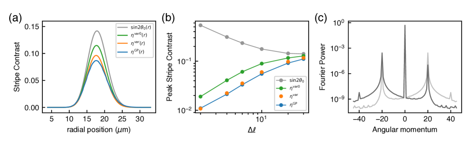
Figure 3: Stripe contrast from the GP and variational calculations with varying $\Delta\ell$. $\Omega_{M}=\Omega_{c}$, $r_{M}=17{\ \mu{\rm m}},R_{\rm TF}=46{\ \mu{\rm m}}$ and $\mu/h=21$ Hz. (a) Contrast versus radial position $r$ for $\Delta\ell=20$. From variational solutions: $\sin 2\theta_{0}(r)$ for non-interacting atoms (grey curve), $\eta^{\rm var0}(r)$ for using two-quasiangular-momentum ansatz (green), and $\eta^{\rm var}(r)$ for using four-quasiangular-momentum ansatz (orange). Blue curve indicates $\eta^{\rm GP}(r)$ for the GP. (b) Peak values of the contrast vs. $\Delta\ell$. Grey, green, orange, and blue symbols denote $\sin 2\theta_{0},\eta^{\rm var0},\eta^{\rm var},\eta^{\rm GP}$, respectively. (c) Annular Fourier power spectrum after integration along $r$ for $\left\lvert\downarrow\right\rangle$ (dark grey) and $\left\lvert\uparrow\right\rangle$ (light grey).

By expanding $A_{\pm}^{\rm var}$ to first order in $\bar{n}g_{1}/E_{L}$ and $\hbar\Omega/E_{L}$, we obtain $A_{\pm}^{\rm var}\approx\bar{n}g_{1}\theta/\sqrt{2}E_{L}$, which also agrees with the result using perturbation (see appendix). After plugging it into Eq. (57), we have

$$\theta^{\rm var}\approx\frac{\hbar\Omega}{2E_{L}}(1-\frac{\bar{n}g_{1}}{E_{L}}),\eta^{\rm var}\approx\frac{\hbar\Omega}{E_{L}}(1-2\frac{\bar{n}g_{1}}{E_{L}}).$$ (58)

Comparing to $\eta^{\rm var0}$ in Eq. (54), we find the coefficient of $\bar{n}g_{1}/E_{L}$ in $\eta^{\rm var}$ is $-2$, twice as that in $\eta^{\rm var0}$. Including the additional OAM $\ell=\pm 3\Delta\ell/2$ in Eq. (24) is necessary for correct results to first order in $\bar{n}g_{1}/E_{L}$. For the separated phase with $C_{+}=1,C_{-}=0$ with $A_{+}=A_{-}=0$, it is identical to that using the two-quasiangular-momentum ansatz.

We comment on earlier theoretical papers on SOAMC systems Sun et al. (2015); Chen et al. (2016, 2019). We examine the peak dimensionless interaction strength $\bar{n}g_{1}/E_{L}$ in these papers. In Ref. Chen et al. (2016), $\bar{n}g_{1}/E_{L}$ is $\lesssim 0.01$, and single-particle eigenstates are taken as the basis of the variational method, i.e., $\theta=\theta_{0}$. Refs. Sun et al. (2015); Chen et al. (2019) use variational methods with the wave function ansatz Eq. (8), where Ref. Sun et al. (2015) has ring traps with $\bar{n}g_{1}/E_{L}>100$, and the interaction $\bar{n}g_{1}$ is not specified In Ref. Chen et al. (2019).

IV Results and discussions

We consider practical experimental parameters to maximize the density contrast of the stripe phase. We first discuss BECs in harmonic traps in the Thomas-Fermi regime along the radial direction with the Thomas-Fermi radius $R_{\rm TF}$. We study how the GP stripe phase contrast depends on ($\Delta\ell,r_{M},R_{\rm TF},\mu$); $\mu$ is the chemical potential and the peak mean field energy in the harmonic trap.

For comparisons, we also consider atoms in ring traps. Here $r_{M}=r_{0}$ is the only length scale, unlike the harmonically trapped systems where there are two relevant length scales, ($r_{M},R_{\rm TF}$).

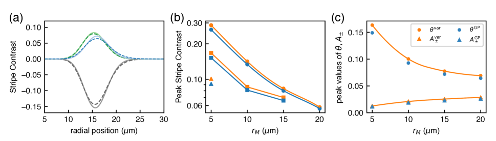
Figure 4: Stripe contrast and $\theta,A_{\pm}$ of the variational results using four-quasiangular-momentum ansatz and of GP with varying ($r_{M},R_{\rm TF}$). $\Omega_{M}=\Omega_{c}$, $\Delta\ell=20$ and $\mu/h=93$ Hz. (a) Comparison of the contrast $\eta$ vs. $r$ for $r_{M}=15{\ \mu{\rm m}}$ and $R_{\rm TF}=50{\ \mu{\rm m}}$. Grey, blue and green curves indicate $-\sin 2\theta$, $2\sqrt{2}\cos\theta A_{\pm}$ and $\eta$, respectively. Solid (dashed) curves denote the variational (GP) simulations. (b) Peak contrast vs. $r_{M}$. Orange (blue) symbols indicate $\eta^{\rm var}(\eta^{\rm GP})$. Circles, squares and triangles for $R_{\rm TF}=50,25,12.5{\ \mu{\rm m}}$, respectively. (c) Peak values of $\theta,A_{\pm}$ vs. $r_{M}$ for $R_{\rm TF}=50{\ \mu{\rm m}}$. Orange (blue) symbols indicate the variational (GP) results; circles (triangles) for $\theta(A_{\pm})$.

IV.1 Harmonic traps

We first obtain the GP ground state phase diagram as shown in Fig. 1c. We then focus on the GP stripe phase at $\delta=0$, setting $\Omega_{M}=\Omega_{c}$. We run simulations for $\Delta\ell$ between 2 and 30, all with $r_{M}=17~{}\mu$m, $R_{\rm TF}=46~{}\mu$m, and $\mu=h\times 21~{}$Hz. $\Delta\ell=30$ corresponds to the LG beam with phase winding number of $\pm 15$, which can be achieved experimentally (in Ref. Tammuz (2011), LG beams with phase winding number of 45 are realized). From the GP wave function $\psi(r,\phi)$, we evaluate the density contrast $\eta^{\rm GP}(r)$ from the normalized Fourier components $\tilde{\psi}$ of $\psi(r,\phi)$ following Eq. (39). For $\left\lvert\downarrow\right\rangle$, $\tilde{\psi}_{\ell_{\downarrow},\downarrow}$ are given by [see Eq. (24)]

$$\tilde{\psi}_{0,\downarrow}=-C_{+}\cos\theta^{\rm GP},\tilde{\psi}_{-20,\downarrow}=-C_{-}\sin\theta^{\rm GP},\tilde{\psi}_{20,\downarrow}=A_{\pm}^{\rm GP},$$ (59)

from which the contrast $\eta_{\downarrow}^{\rm GP}=\eta_{\uparrow}^{\rm GP}\approx|\sin 2\theta^{\rm GP}-2\sqrt{2}\cos\theta^{\rm GP}A_{\pm}^{\rm GP}|$ derived in Eq. (39) can be described as $4\tilde{\psi}_{0,\downarrow}\tilde{\psi}_{-20,\downarrow}$ (the first term) and $4\tilde{\psi}_{0,\downarrow}\tilde{\psi}_{20,\downarrow}$ (the second term). We then compare $\eta^{\rm GP}(r)$ to the variational solutions of the contrast, which are $\sin 2\theta_{0}(r)$ for the non-interacting case, $\eta^{\rm var0}(r)$ for using the two-quasiangular-momentum ansatz [Eq. (53) from the ansatz Eq. (8)] and $\eta^{\rm var}(r)$ for using the four-quasiangular-momentum ansatz [Eq. (57) from the ansatz Eq. (24)]. In Fig. 3a, we plot $\sin 2\theta_{0}(r)$, $\eta^{\rm var0}(r)$, $\eta^{\rm var}(r)$ and $\eta^{\rm GP}(r)$ for the example value $\Delta\ell=20$; their maxima are at $r\gtrsim r_{M}$. In Fig. 3b, We plot the peak values of $\sin 2\theta_{0}(r)$, $\eta^{\rm var0}(r)$, $\eta^{\rm var}(r)$ and $\eta^{\rm GP}(r)$ versus $\Delta\ell$, which are denoted as $\sin 2\theta_{0},~{}\eta^{\rm var0},~{}\eta^{\rm var}$ and $\eta^{\rm GP}$, respectively. We observe that the single-particle contrast $\sin 2\theta_{0}$ is significantly larger than $\eta^{\rm GP}$ for small $\Delta\ell$, while $\sin 2\theta_{0}$ and $\eta^{\rm GP}$ are close for $\Delta\ell\geq 20$. As the dimensionless interaction $\bar{n}g_{1}/E_{L}$ increases with decreasing $\Delta\ell$, the contrast $\eta^{\rm GP}$ decreases. When the interaction is taken into consideration using the ansatz Eq. (8), the resulting $\eta^{\rm var0}$ overestimates $\eta^{\rm GP}$, indicating that Eq. (8) is insufficient. We can understand this from the annular Fourier transform of the GP wave function $\psi_{\downarrow}$ for $\Delta\ell=20$. Fig. 3c shows the power spectrum of the normalized Fourier components $\tilde{\psi}_{\ell_{\downarrow},\downarrow}$, where there are $\ell_{\downarrow}=0,\pm 20$ components, and the $\ell_{\downarrow}=-40$ is negligible since its power is about $10^{-3}$ of that of $\ell_{\downarrow}=20$. The appearance of the $\ell_{\downarrow}=20$ component signifies that the more general Eq. (24) should be used in the variation method with the $A_{+}$ term accounting for $\ell_{\downarrow}=20$, while $A_{+},A_{-}$ are absent in the simple Eq. (8). The spectrum for $\left\lvert\uparrow\right\rangle$ is also displayed in Fig. 3c. The GP results have $C_{\pm}\approx\mp 1/\sqrt{2}$ and $A_{+}=A_{-}=A_{\pm}^{\rm GP}$, which confirms the time-reversal symmetry condition, Eq. (35). [From the GP results, the signs of $C_{\pm}\approx\mp 1/\sqrt{2}$ are applied in Eq. (35) and in the variational method using Eq. (24).] We also show the peak values, $\eta^{\rm var}$ of $\eta^{\rm var}(r)$, in Fig. 3b, where $\eta^{\rm var0}>\eta^{\rm var}\gtrsim\eta^{\rm GP}$ and $\eta^{\rm var}$ fits well with $\eta^{\rm GP}$.

From the above studies, we find the maximum of the stripe contrast is at $r=r_{\rm peak}\approx r_{M}$, where the spatial period is $\approx 2\pi r_{M}/\Delta\ell$. ($r_{\rm peak}$ is only slightly larger than $r_{M}$ for all the contrasts, e.g., $r_{\rm peak}=17.6{\ \mu{\rm m}}$ for $\eta^{\rm GP}$ in Fig. 3a.) The peak value of the contrast increases with $\Delta\ell$, and thus a larger contrast corresponds to a small stripe period $\propto\Delta\ell^{-1}$. To observe the stripe phase in experiments, we note that with state-of-the-art imaging techniques in ultracold atoms, e.g. those using quantum gas microscopes, one can resolve as small as $0.5{\ \mu{\rm m}}$ with $\lambda=0.78{\ \mu{\rm m}}$ for ⁸⁷Rb Bakr et al. (2009). This sets the lower bound on $2\pi r_{M}/\Delta\ell$ in our simulations. Since the peak contrast is the signal we optimize, $r_{\rm peak}\approx r_{M}$ and thus $E_{L}(r_{\rm peak})\approx E_{L}(r_{M})$ are the relevant length and energy scale for SOAMC, respectively.

Next, we fix $\Delta\ell=20$ and $\mu=h\times 93~{}$Hz, and vary $(r_{M},R_{\rm TF})$. We study $r_{M}<R_{\rm TF}$ where there is sufficient atomic density at $r=r_{M}$ for various combinations of $(r_{M},R_{\rm TF})$. Here we set the smallest $r_{M}=5~{}\mu$m for $\Delta\ell=20$, where the spatial period of the stripe is $\approx 1.6{\ \mu{\rm m}}$ and is larger than the diffraction limit of the imaging, $0.5{\ \mu{\rm m}}$. With $\Omega_{M}=\Omega_{c}$, the GP results have the peak contrast $\eta^{\rm GP}$ increasing with decreasing $r_{M}$ and increasing $R_{\rm TF}$, as shown in Fig. 4b. We then compare the GP to the variational calculations with four-quasiangular-momentum ansatz . In Fig. 4a, we plot the density contrast contributed from $\theta,A_{\pm}$ and the sum, respectively. These are $-\sin 2\theta^{\rm GP}$, $2\sqrt{2}\cos\theta^{\rm GP}A_{\pm}^{\rm GP}$, and $\eta^{\rm GP}$ versus $r$ for GP, and $-\sin 2\theta^{\rm var}$, $2\sqrt{2}\cos\theta^{\rm var}A_{\pm}^{\rm var}$, and $\eta^{\rm var}$ versus $r$ for the variational calculations. We find the contrast of GP obtained from Eq. (13) versus $r$ agrees well with $\eta^{\rm GP}(r)$, showing that $\eta^{\rm GP}$ from the $\cos(\Delta\ell\phi)$ term dominates the contrast in Eq. (II), where the second harmonics is negligible. We display the peak values $\eta^{\rm var}$ versus $r_{M}$ for all $R_{\rm TF}$ in Fig. 4b and compare them to the peak values $\eta^{\rm GP}$, where $\eta^{\rm var}$ overestimates $\eta^{\rm GP}$ by $3-8~{}\%$. For all ($r_{M},R_{\rm TF}$), the Fourier spectrum of GP has $\ell_{\uparrow,\downarrow}=0,\pm 20$ components and $\ell_{\uparrow}=40,\ell_{\downarrow}=-40$ are negligible, being consistent with Eq. (24). We then compare the peak values $(\theta^{\rm GP},A_{\pm}^{\rm GP})$ to $(\theta^{\rm var},A_{\pm}^{\rm var})$ versus $r_{M}$ for $R_{\rm TF}=50~{}\mu$m in Fig. 4c. The peaks of $\theta$ and $A_{\pm}$ are at $r\approx r_{M}$, as well as that of the contrast $\eta$. $\theta^{\rm var}$ and $A_{\pm}^{\rm var}$ slightly overestimate $\theta^{\rm GP}$ and $A_{\pm}^{\rm GP}$, respectively: both $\theta^{\rm GP}/\theta^{\rm var}$ and $A_{\pm}^{\rm GP}/A_{\pm}^{\rm var}$ are between $0.90-0.93$. This is attributed to the radial kinetic energy that is neglected in the variational calculations. The GP ground state has smaller $(\theta^{\rm GP},A_{\pm}^{\rm GP})$ than $(\theta^{\rm var},A_{\pm}^{\rm var})$ where the smaller radial spin gradient corresponds to a smaller radial kinetic energy, and thus the lowest overall energy.

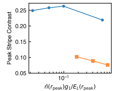
Figure 5: Peak stripe contrast $\eta^{\rm GP}$ versus interaction strength $\bar{n}(r_{\rm peak})g_{1}/E_{L}(r_{\rm peak})$ with varying $\mu$, $\Delta\ell=20$ and $R_{\rm TF}=50~{}\mu$m. Circles and square symbols indicate $r_{M}=5,15~{}\mu$m, respectively.

After studying the dependence of the peak contrast $\eta^{\rm GP}$ on ($\Delta\ell,r_{M},R_{\rm TF}$), we vary $\mu$ and thus the interaction strength $\bar{n}g_{1}/E_{L}$ at $r=r_{\rm peak}\approx r_{M}$ , $\bar{n}g_{1}/E_{L}=\mu\left[1-(r_{\rm peak}/R_{\rm TF})^{2}\right]/E_{L}(r_{\rm peak})$. We fix $\Delta\ell=20,R_{\rm TF}=50{\ \mu{\rm m}}$ for $r_{M}=5$ and $15{\ \mu{\rm m}}$, respectively. We study $\mu=h\times 21,46,93$ Hz for both $r_{M}$, and additionally $\mu=h\times 600$ Hz for $r_{M}=5{\ \mu{\rm m}}$. Fig. 5 shows $\eta^{\rm GP}$ weakly depends on $\bar{n}g_{1}/E_{L}$.

Besides the density contrast, we compare the critical coupling $\Omega_{c}$ of the GP results to those given by the variational methods. Using the two-quasiangular-momentum ansatz, Eq. (8), the critical coupling $\Omega_{c}^{\rm var0}$ is given by

$$\int dr2\pi r\bar{n}(r)\Delta\varepsilon^{\rm var0}=0,$$

$$\Delta\varepsilon^{\rm var0}=\varepsilon^{\rm var0}(\theta^{\rm var0},\beta=1/4)-\varepsilon_{\rm sep}.$$ (60)

$\Delta\varepsilon^{\rm var0}$ is the energy difference between the stripe phase and the separated phase, $\theta^{\rm var0}$ is the variational solution of $\theta$ for the stripe phase, and $\varepsilon_{\rm sep}$ is the energy of the separated phase with $\theta=\theta_{\rm sep}$ and $\beta=0$. When the integral is $<(>)~{}0$ at $\Omega_{M}<(>)\Omega_{c}$, the ground state is the stripe (separated) phase. Similarly, by using the four-quasiangular-momentum ansatz, Eq. (24), the critical coupling $\Omega_{c}^{\rm var}$ is given by

$$\int dr2\pi r\bar{n}(r)\Delta\varepsilon^{\rm var}=0,$$

$$\Delta\varepsilon^{\rm var}=\varepsilon^{\rm var}(\theta^{\rm var},C_{\pm}=\mp\sqrt{\left[1-2(A^{\rm var}_{\pm})^{2}\right]/2})-\varepsilon_{\rm sep}.$$ (61)

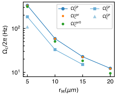
Figure 6: Critical coupling $\Omega_{c}$ vs. $r_{M}$ with various $R_{\rm TF}$ of GP and variational results from two-quasiangular-momentum and four-quasiangular-momentum ansatz. Blue symbols denote $\Omega_{c}^{\rm GP}$; circles, squares and triangle for $R_{\rm TF}=50,25,12.5{\ \mu{\rm m}}$, respectively. Orange (green) symbols indicate $\Omega_{c}^{\rm var}(\Omega_{c}^{\rm var0})$ for $R_{\rm TF}=50{\ \mu{\rm m}}$.

In Fig. 6, we plot $\Omega_{c}$ of the GP and from the solutions of Eq. (IV.1) and Eq. (IV.1) versus $(r_{M},R_{\rm TF})$, where $\Omega_{c}$ from GP have good agreements with $\Omega_{c}^{\rm var}$.

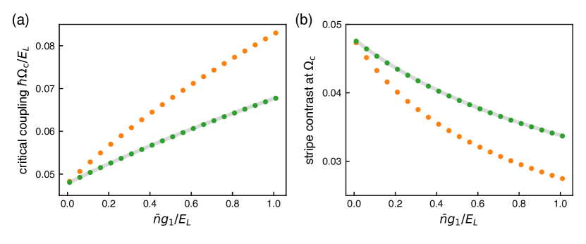
Figure 7: Critical coupling $\hbar\Omega_{c}/E_{L}$ and stripe contrast $\eta$ at $\Omega_{c}$ vs. $\bar{n}g_{1}/E_{L}$ at fixed $r$. Variational calculations of two-quasiangular-momentum and four-quasiangular-momentum ansatz for SOAMC, and of two-quasilinear-momentum ansatz for SLMC are illustrated. Green symbols, orange symbols and grey curve display $\hbar\Omega_{c}^{\rm var0}/E_{L},\hbar\Omega_{c}^{\rm var}/E_{L}$ and $\hbar\Omega_{c}^{\rm SLMC}/E_{L}$, respectively for (a), and display $\eta^{\rm var0},\eta^{\rm var}$ and $\eta^{\rm SLMC}$ for (b).

We can understand that $\Omega_{c}$ increases with increasing $R_{\rm TF}$ and decreasing $r_{M}$ from a geometric argument. Such dependence on ($r_{M},R_{\rm TF}$) is crucial since a larger $\hbar\Omega_{c}/E_{L}$ leads to larger stripe contrast $\eta^{\rm var}$, see Eq. (58). We find numerically that the energy difference between the stripe phase and separated phase can be written as

$$\Delta\varepsilon^{\rm var} =f(r)-\frac{\bar{n}(r)g_{2}}{2},$$

$$f(r) =\bar{n}(r)g_{1}H(\frac{\bar{n}g_{1}}{E_{L}})\frac{\hbar^{2}\Omega^{2}(r)}{E_{L}^{2}}$$ (62)

for small $\theta$, where $H$ is a dimensionless function of $\bar{n}g_{1}/E_{L}$ and $H\rightarrow 1/4$ as $\bar{n}g_{1}/E_{L}\rightarrow 0$. To make a geometric analysis, we simplify $f(r)$ as a flat impulse function centered at $r=r_{M}$ with full width $\Delta r=(\Delta\ell/2)^{-1/2}r_{M}$,

$$f(r) =f_{M},r_{M}-\Delta r/2<r<r_{M}+\Delta r/2,$$

$$f_{M} =\bar{n}g_{1}H(\frac{\bar{n}g_{1}}{E_{L}})\frac{\hbar^{2}\Omega_{M}^{2}}{E_{L}^{2}},$$ (63)

where $\bar{n}g_{1},E_{L}$ and $\Omega_{M}$ are evaluated at $r=r_{M}$, approximately the peak position of $f(r)$. Assuming a cylindrical box trap with uniform $\bar{n}$ within $r=R_{\rm box}$, the integral in Eq. (IV.1) then gives

$$\bar{n}2\pi r_{M}\Delta rf_{M}=\bar{n}\pi R_{\rm box}^{2}\frac{\bar{n}g_{2}}{2},$$

and thus

$$f_{M}=\frac{\bar{n}g_{2}}{2}\left(\frac{\pi R_{\rm box}^{2}}{2\pi r_{M}\Delta r}\right),$$ (64)

where the number in the parentheses is an area ratio of the box to that of the distribution $f(r)$. From Eq. (IV.1) and Eq. (64) and assuming a fixed interaction strength $\bar{n}g_{1}/E_{L}$, we obtain $\Omega_{M}=\Omega_{c}\propto R_{\rm box}r_{M}^{-3}$ which increases with increasing $R_{\rm box}$ and decreasing $r_{M}$.

IV.2 Ring traps

We show the variational results for the ring trap versus the dimensionless interaction strength $g_{1}^{\prime}=\bar{n}g_{1}/E_{L}(r_{0})$. These are the solutions of the critical coupling $\Omega_{c}$ and the contrast at $\Omega_{c}$. We solve the dimensionless critical coupling $\Omega_{c}^{\prime}=\hbar\Omega_{c}/E_{L}$ by using $\Delta\varepsilon^{\rm var0}(r_{0})=0$ and $\Delta\varepsilon^{\rm var}(r_{0})=0$, respectively, and plot $\Omega_{c}^{\prime}$ vs. $g_{1}^{\prime}$ in Fig. 7a. $\Omega_{c}^{\rm var}$ exceeds $\Omega_{c}^{\rm var0}$ for $g_{1}^{\prime}>0$, and $\hbar\Omega_{c}^{\rm var0}\approx\hbar\Omega_{c}^{\rm var}\rightarrow\sqrt{2g_{2}/g_{1}}~{}E_{L}\approx 0.05~{}E_{L}$ as $g_{1}^{\prime}\rightarrow 0$. we can understand $\Omega_{c}^{\rm var}>\Omega_{c}^{\rm var0}$ as the following: At a given $\Omega$, the stripe phase energy is $\varepsilon^{\rm var}<\varepsilon^{\rm var0}$ since the smaller contrast $\eta^{\rm var}$ [see Eq. (54) and Eq. (58)] corresponds to smaller interaction energy. Therefore, the critical coupling determined by $\Delta\varepsilon=0$, where $\Delta\varepsilon$ increases with $\Omega$, is shifted to a larger value for $\Omega_{c}^{\rm var}$. In the $g_{1}^{\prime}\rightarrow 0$ limit, $\Delta\varepsilon^{\rm var0}(r_{0})\approx\Delta\varepsilon^{\rm var}(r_{0})$, where the stripe and separated phases have approximately the same variational solution, $\theta^{\rm var0}\approx\theta_{\rm sep}\approx\theta_{0}$, and thus $\Delta\varepsilon^{\rm var0}=(1/4)\bar{n}\left[g_{1}\sin^{2}2\theta_{0}-2g_{2}\cos^{2}2\theta_{0}\right]=0$ from Eq. (50), leading to $\Omega_{c}^{\prime}=\sqrt{2g_{2}/g_{1}}$. The stripe contrasts $\eta^{\rm var0}$ and $\eta^{\rm var}$ at respective $\Omega_{c}$ are displayed in Fig. 7b; they are $\approx 5~{}\%$ as $g_{1}^{\prime}\rightarrow 0$, both decreasing with increasing $g_{1}^{\prime}$ and $\eta^{\rm var}<\eta^{\rm var0}$. To compare with SLMC systems, $\hbar\Omega_{c}^{\rm var0}/E_{L}$ for $g_{1}^{\prime}<1$ agrees well with that of SLMC (see Fig. 7a), which is $\hbar\Omega_{c}^{\rm SLMC}/4E_{r}=\sqrt{2g_{2}/g_{1}}$ as $g_{1}^{\prime}\rightarrow 0$ Li et al. (2012), i.e., $\hbar\Omega_{c}^{\rm SLMC}=0.2E_{r}$; $4E_{r}$ is equivalent to $E_{L}$ for SOAMC.

The spin-dependent interaction strength $g_{2}/g_{1}$ determines the critical coupling $\hbar\Omega_{c}/E_{L}$ and stripe contrast $\eta$ as $g_{1}^{\prime}\rightarrow 0$; larger $g_{2}/g_{1}$ gives larger $\hbar\Omega_{c}/E_{L}$ and $\eta$, i.e., larger miscibility. The contrast of SLMC also agrees well with $\eta^{\rm var0}$, see Fig. 7b. We find that $\Omega_{c}^{\prime}$ and $\eta$ of SOAMC with $\varepsilon^{\rm var0}$ and of SLMC, where both are based on Eq. (8), are incorrect to first order in $g_{1}^{\prime}$. By including higher order OAM in Eq. (24), the result is correct to first order, as indicated by Eq. (54) and Eq. (58). The stripe contrast of SOAMC is at most $\approx 5~{}\%$ in the $g_{1}^{\prime}\rightarrow 0$ limit, and it is independent of either the ring radius $r_{0}$ or $\Delta\ell$. On the other hand, a stripe contrast $\lesssim 30~{}\%$ for harmonic traps is achieved with a relatively large $R_{\rm TF}=50{\ \mu{\rm m}}$ and a relatively small $r_{M}=5{\ \mu{\rm m}}$, and this can be understood from the geometric analysis as shown in Eq. (64).

We then perform GP simulations for a ring trap with $r_{0}=r_{M}=10{\ \mu{\rm m}}$ and $\Delta\ell=20$. The atoms are in an annular box potential within $8{\ \mu{\rm m}}<r<12{\ \mu{\rm m}}$, and $\bar{n}g_{1}/E_{L}=0.63$ at $r=r_{0}$. The GP result has good agreement with the variational calculation, where $\theta^{\rm GP}/\theta^{\rm var}=0.95$ and $A_{\pm}^{\rm GP}/A_{\pm}^{\rm var}=0.91$.

V Conclusions

In summary, we optimize the density contrast of the ground state stripe phase of ⁸⁷Rb SOAMC BECs by tuning experimental parameters. A contrast of nearly $30~{}\%$ is achieved for atoms in harmonic traps; and a larger contrast of about $50~{}\%$ is expected by using a twice larger BEC cloud size based on variational calculations. Such high contrasts are achieved owing to the geometry with two length scales in harmonic traps, the Raman Laguerre-Gaussian beam size and the BEC cloud size. While for ring traps, these two scales are the same, leading to maximal contrast about $5~{}\%$, which is dictated by the spin-dependent interaction strength and is the same as that of the SLMC systems. For both atoms in harmonic traps and ring traps, we perform GP simulations and variational calculations based on the two-quasiangular-momentum ansatz and four-quasiangular-momentum ansatz. We find the results from the simple two-quasiangular-momentum ansatz, which is used in previous papers Li et al. (2012); Sun et al. (2015); Chen et al. (2016, 2019), is consistent with the GP results only in the non-interacting limit. With small interactions, high order OAM components must be included as the four-quasiangular-momentum ansatz; this then leads to correct results to first order in interaction and good agreements with the GP simulations.

We point out that one can improve the stability by using the synthetic clock states instead of bare spin states. The clock states are immune to detuning variations arising from the bias field variations. A $0.1-1$ Hz stability of the clock transition frequency is achieved as shown in Ref. Trypogeorgos et al. (2018). Thus, the ground state stripe phase within a narrow detuning window of about $1$ Hz may be observed for ⁸⁷Rb atoms with mean field energy about 1 kHz. The spin-dependent interaction strength in the clock state basis is close to the $g_{2}/g_{1}$ for bare spin states (see appendix), leading to similar magnitude of stripe contrast to our simulations using bares spin states. We envision our work to pave the way toward a direct observation of high-contrast stripe phases in spin-orbital-angular-momentum coupled Bose-Einstein condensates, achieving a long-standing goal in quantum gases.

VI Appendix

VI.1 Spinor wave function ansatz

We show that the spinor wave function ansatz Eq. (24) is valid for small $\theta$ (given small Raman coupling $\hbar\Omega/E_{L}$) and small interaction $\bar{n}g_{1}/E_{L}$. The GPE for $\left\lvert\uparrow\right\rangle,\left\lvert\downarrow\right\rangle$ with $\delta=0$ is

$$(-\frac{\hbar^{2}}{2m}\nabla^{2}+g|\psi_{\uparrow}|^{2}+g_{\uparrow\downarrow}|\psi_{\downarrow}|^{2}-\mu_{\uparrow})\psi_{\uparrow}+\frac{\hbar\Omega(r)}{2}e^{i\Delta\ell\phi}\psi_{\downarrow}=0,$$ (65a)

$$(-\frac{\hbar^{2}}{2m}\nabla^{2}+g|\psi_{\downarrow}|^{2}+g_{\uparrow\downarrow}|\psi_{\uparrow}|^{2}-\mu_{\downarrow})\psi_{\downarrow}+\frac{\hbar\Omega(r)}{2}e^{-i\Delta\ell\phi}\psi_{\uparrow}=0.$$ (65b)

Here we set $V(r)=0$ to simplify the discussion. For the spatially-mixed stripe phase ground state, $\mu_{\uparrow}=\mu_{\downarrow}$. Next we show the nonlinear interaction leads to multiple OAM components in the spinor wave function ansatz. With $\ell=\Delta\ell/2=10$, we plug $\psi_{\uparrow}=\sqrt{\bar{n}(r)}\left(C_{+}\sin\theta e^{i20\phi}+C_{-}\cos\theta\right),\psi_{\downarrow}=\sqrt{\bar{n}(r)}\left(-C_{+}\cos\theta-C_{-}\sin\theta e^{-i20\phi}\right)$ from Eq. (8) into Eq. (65a), neglect radial gradients and keep the expansion terms up to $\theta^{2}$. The nonlinear interaction terms for $\psi_{\uparrow}$ are

$$g|\psi_{\uparrow}|^{2}\psi_{\uparrow}+g_{\uparrow\downarrow}|\psi_{\downarrow}|^{2}\psi_{\uparrow} =\sqrt{\bar{n}}^{3}[C_{-}C_{+}^{2}(g+g_{\uparrow\downarrow})\theta^{2}e^{i40\phi}$$

$$+C_{+}\left(2C_{-}^{2}g+g_{\uparrow\downarrow}\right)\theta e^{i20\phi}$$

$$+C_{-}\left(C_{-}^{2}g+C_{+}^{2}g_{\uparrow\downarrow}+O[\theta^{2}]\right)$$

$$+C_{-}^{2}C_{+}\left(g+g_{\uparrow\downarrow}\right)\theta e^{-i20\phi}].$$ (66)

Besides $\ell_{\uparrow}=0,20$, additional OAM terms with $\ell_{\uparrow}=-20,40$ appear due to the nonlinear interaction, which are of order of $\theta,\theta^{2}$, respectively, and are not included in Eq. (8). By keeping up to order $\theta^{2}$, the spinor wave function has additional variational parameters $A_{+},A_{-},B_{+},B_{-}$, given by

$$\left(\begin{array}[]{c}\psi_{\uparrow}\\ \psi_{\downarrow}\end{array}\right)=\sqrt{\bar{n}(r)}[ e^{i\frac{3\Delta\ell}{2}\phi}\left(\begin{array}[]{c}B_{+}e^{i\frac{\Delta\ell}{2}\phi}\\ A_{+}e^{-i\frac{\Delta\ell}{2}\phi}\end{array}\right)$$ (71)

$$+C_{+}e^{i\frac{\Delta\ell}{2}\phi}\left(\begin{array}[]{c}\sin\theta(r)e^{i\frac{\Delta\ell}{2}\phi}\\ -\cos\theta(r)e^{-i\frac{\Delta\ell}{2}\phi}\end{array}\right)$$ (74)

$$+C_{-}e^{-i\frac{\Delta\ell}{2}\phi}\left(\begin{array}[]{c}\cos\theta(r)e^{i\frac{\Delta\ell}{2}\phi}\\ -\sin\theta(r)e^{-i\frac{\Delta\ell}{2}\phi}\end{array}\right)$$ (77)

$$+e^{-i\frac{3\Delta\ell}{2}\phi}\left(\begin{array}[]{c}A_{-}e^{i\frac{\Delta\ell}{2}\phi}\\ B_{-}e^{-i\frac{\Delta\ell}{2}\phi}\end{array}\right)].$$ (80)

$\ell_{\uparrow}=-20$ is of order $\theta$ and corresponds to $\ell=-3\Delta\ell/2=-30$ with $A_{-}$; $\ell_{\uparrow}=40$ is of order $\theta^{2}$ and corresponds to $\ell=3\Delta\ell/2=30$ with $B_{+}$. For small $\theta$, by taking up to order $\theta$ we have the spinor wave function ansatz Eq. (24) with $A_{+},A_{-}\neq 0$ and $B_{+}=B_{-}=0$.

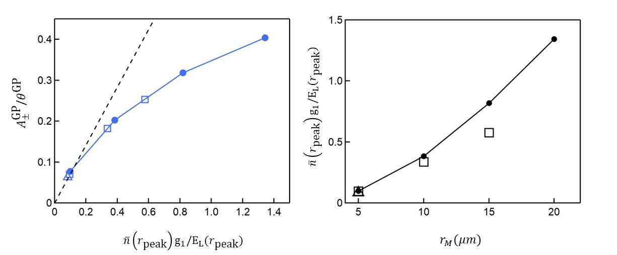
Figure 8: (a) Ratio of the peak values $A_{\pm}^{\rm GP}/\theta^{\rm GP}$ of GP stripe phase versus the interaction evaluated at $r_{\rm peak}$, $\bar{n}(r_{\rm peak})g_{1}/E_{L}(r_{\rm peak})$. Circles for $R_{\rm TF}=50{\ \mu{\rm m}}$, open squares for $25{\ \mu{\rm m}}$, and open triangle for $12.5{\ \mu{\rm m}}$; $r_{\rm peak}\approx r_{M}$. (b) $\bar{n}(r_{\rm peak})g_{1}/E_{L}(r_{\rm peak})$ versus $r_{M}$ for $R_{\rm TF}=50{\ \mu{\rm m}}$, $25{\ \mu{\rm m}}$, and $12.5{\ \mu{\rm m}}$. Same symbols as (a) and all with $\mu/h=93$ Hz.

Next we derive $A_{-}$ for small interactions $\bar{n}g_{1}/E_{L}$ using first order perturbation. We plug

$$\psi_{\uparrow} =\sqrt{\bar{n}}\left(C_{+}\sin\theta e^{i20\phi}+C_{-}\cos\theta+A_{-}e^{-i20\phi}\right),$$

$$\psi_{\downarrow} =\sqrt{\bar{n}}\left(A_{+}e^{i20\phi}-C_{+}\cos\theta-C_{-}\sin\theta e^{-i20\phi}\right)$$ (81)

into Eq. (65a) for $\psi_{\uparrow}$, and focus on the coefficient of the $e^{-i20\phi}$ term, which is

$$\left(E_{L}-\mu_{\uparrow}\right)\sqrt{\bar{n}}A_{-}+\sqrt{\bar{n}}^{3}C_{-}^{2}C_{+}\left(g+g_{\uparrow\downarrow}\right)\theta=0.$$ (82)

Besides reading out from Eq. (VI.1), the coefficient of the $e^{-i20\phi}$ term in the nonlinear interaction $g|\psi_{\uparrow}|^{2}\psi_{\uparrow}+g_{\uparrow\downarrow}|\psi_{\downarrow}|^{2}\psi_{\uparrow}$ can be readily found from the Fourier components of $|\psi_{\uparrow}|^{2},|\psi_{\downarrow}|^{2}$ in Eq. (II), both of which have OAM$=0,\pm 20$. Then, using $\mu_{\uparrow}\approx\mu_{\uparrow}(\Omega=0,g=g_{\uparrow\downarrow}=0)=0$ for small $\Omega/E_{L}$ and $\bar{n}g_{1}/E_{L}$, along with $C_{\pm}\approx\mp 1/\sqrt{2}$, it gives

$$A_{-}\approx\frac{\bar{n}g_{1}}{\sqrt{2}E_{L}}\theta.$$ (83)

From the GP stripe phase wave function, in Fig. 8a we plot the ratio of the peak values $A_{\pm}^{\rm GP}/\theta^{\rm GP}$ vs. $\bar{n}(r_{\rm peak})g_{1}/E_{L}(r_{\rm peak})$, along with the ratio $\bar{n}g_{1}/\sqrt{2}E_{L}$ given by Eq. (83), which agrees with $A_{\pm}^{\rm GP}/\theta^{\rm GP}$ at small $\bar{n}(r_{\rm peak})g_{1}/E_{L}(r_{\rm peak})$. The dimensionless interaction $\bar{n}g_{1}/E_{L}$ evaluated at $r_{\rm peak}\approx r_{M}$ vs. $r_{M}$ for $R_{\rm TF}=12.5,25,50{\ \mu{\rm m}}$ is shown in Fig. 8b, all with $\mu=h\times 93$ Hz. For a fixed $\mu$, $\bar{n}g_{1}=\mu[1-(r/R_{\rm TF})^{2}]$ weakly depends on $r$ for $r/R_{\rm TF}\lesssim 0.5$. $\bar{n}(r_{\rm peak})g_{1}/E_{L}(r_{\rm peak})$ increases with increasing $r_{M}$, which is dominated by $E_{L}\propto r^{-2}$.

Similarly, we derive $B_{+}$ by plugging

$$\psi_{\uparrow} =\sqrt{\bar{n}}\left(B_{+}e^{i40\phi}+C_{+}\sin\theta e^{i20\phi}+C_{-}\cos\theta+A_{-}e^{-i20\phi}\right),$$

$$\psi_{\downarrow} =\sqrt{\bar{n}}\left(A_{+}e^{i20\phi}-C_{+}\cos\theta-C_{-}\sin\theta e^{-i20\phi}+B_{-}e^{-i40\phi}\right)$$ (84)

into Eq. (65a). The coefficient of the $e^{i40\phi}$ term is

$$\left(4E_{L}-\mu_{\uparrow}\right)\sqrt{\bar{n}}B_{+}+\frac{\hbar\Omega}{2}\sqrt{\bar{n}}A_{+}+\sqrt{\bar{n}}^{3}C_{-}C_{+}^{2}\left(g+g_{\uparrow\downarrow}\right)\theta^{2}=0.$$ (85)

With $\theta\approx\hbar\Omega/2E_{L}(1-\bar{n}g_{1}/E_{L})$ from $\theta^{\rm var}$, and $A_{+}=A_{-}$ for the ground state, it leads to

$$B_{+}\approx-\left(\frac{\hbar\Omega}{8E_{L}}\frac{\bar{n}g_{1}}{\sqrt{2}E_{L}}\theta+\frac{\bar{n}g_{1}}{4\sqrt{2}E_{L}}\theta^{2}\right)\approx-\frac{\bar{n}g_{1}}{2\sqrt{2}E_{L}}\theta^{2}.$$ (86)

In our GP data, the peak values of $B_{\pm}^{\rm GP}$ at $r\gtrsim r_{M}$ are small, $0.02<B_{\pm}^{\rm GP}/A_{\pm}^{\rm GP}<0.04$ for $\bar{n}(r_{\rm peak})g_{1}/E_{L}(r_{\rm peak})<2$. Thus it is valid to neglect $B_{\pm}$ by using the wave function ansatz Eq. (24). We have small $\theta^{\rm GP}$, $0.05<\theta^{\rm GP}<0.16$, and small interaction, $\bar{n}(r_{\rm peak})g_{1}/E_{L}(r_{\rm peak})<2$ except for the data with the smallest $\Delta\ell=2,4$ in Fig. 3.

VI.2 Methods for GP ground state simulations

We run the GP simulations with both the open-source GPELab toolbox Antoine and Duboscq (2014) and Crank-Nicolson method. The grid size is between $0.11-0.55{\ \mu{\rm m}}$ depending on the spatial resolution we need.

To do analysis of the GP wave function in the cylindrical coordinate, we first make interpolations of the raw data in the cartesian coordinate. The annular Fourier transform is performed as

$$\psi_{m}(r,\phi)=\sum_{q^{\prime}}\psi_{q^{\prime},m}(r)e^{iq^{\prime}\phi},$$

$$\psi_{q,m}=(2\pi)^{-1}\int d\phi\psi_{m}(r,\phi)e^{-iq\phi},$$ (87)

where $q=\ell_{\uparrow},\ell_{\downarrow}$ is the OAM and $m=\uparrow,\downarrow$ is the spin label. For the stripe phase with $\bar{n}_{\uparrow}(r)=\bar{n}_{\downarrow}(r)=\bar{n}(r)/2$,

$$\sum_{q}|\psi_{q,m}(r)|^{2}=\bar{n}(r)/2.$$ (88)

We take the normalized Fourier components as $\tilde{\psi}_{q,m}(r)=\psi_{q,m}(r)\bar{n}(r)^{-1/2}$, leading to $\tilde{\psi}_{0,\downarrow}=-C_{+}\cos\theta^{\rm GP},\tilde{\psi}_{-20,\downarrow}=-C_{-}\sin\theta^{\rm GP},\tilde{\psi}_{20,\downarrow}=A_{\pm}^{\rm GP}$. The power spectrum in Fig. 3c is after the integration along $r$,

$$n_{q,m}\propto\int drr|\tilde{\psi}_{q,m}(r)|^{2},\sum_{q,m}n_{q,m}=1.$$ (89)

VI.3 Variational calculations

We consider the SOAMC ground state as either the stripe phase with $|C_{+}C_{-}|>0$ or the separated phase with $|C_{+}C_{-}|=0$, i.e., $C_{+}=1,C_{-}=0$ or $C_{-}=1,C_{+}=0$. The former corresponds to a density stripe and the latter to no density stripe. In the variational calculation using two-quasiangular-momentum ansatz where $A_{\pm}$ is absent in the wave function, $0\leq\beta=|C_{+}|^{2}|C_{-}|^{2}\leq 1/4$ and $\beta=1/4$ corresponds to $|C_{+}|^{2}=|C_{-}|^{2}=|C_{+}C_{-}|=1/2$. We compare the energy of $\beta=1/4$ and of $\beta=0$, and take the lower one as the ground state. This is valid because the lowest energy is at either $\beta=1/4$ or $\beta=0$, i.e., no energy maximum within $0\leq\beta=|C_{+}|^{2}|C_{-}|^{2}\leq 1/4$. We find this condition holds by numerically checking the second order derivative of $\varepsilon^{\rm var0}$, which is negative for $0\leq\beta\leq 1/4$ and $\bar{n}g_{1}/E_{L}<2$. As for the calculation using four-quasiangular-momentum ansatz for the stripe phase, we compare the energy $\varepsilon^{\rm var}$ of the stripe phase, $C_{\pm}=\mp\sqrt{(1-2A_{\pm}^{2})/2}$, and of the separated phase with $C_{+}=1,C_{-}=0,A_{\pm}=0$. It is valid to take $C_{\pm}=\mp\sqrt{(1-2A_{\pm}^{2})/2}$ for the stripe phase since the GP results confirm that this condition holds, which has the time reversal symmetry, Eq. (35).

VI.4 Trap parameters of the simulations

We indicate the trap parameters: for data in Fig. 3 with $\mu=h\times 21$ Hz and $R_{\rm TF}=46{\ \mu{\rm m}}$, $N=10^{4},\omega_{r}/2\pi=1.5$ Hz, and $\omega_{z}/2\pi=600$ Hz. For data in Fig. 4 with $\mu=h\times 93$ Hz and $R_{\rm TF}=12.5,25,50{\ \mu{\rm m}}$, $N=0.25\times 10^{4},10^{4},4\times 10^{4},\omega_{r}/2\pi=11.744,5.872,2.936$ Hz respectively; $\omega_{z}/2\pi=1000$ Hz.

VI.5 Comparison to SLMC systems

We list results of spin-linear-momentum coupled (SLMC) BECs from Ref. Li et al. (2012). Two counter-propagating Raman beams along $x$ transfer linear momentum $\Delta k_{x}=2k_{r}$ between spin $\left\lvert\uparrow\right\rangle$ and $\left\lvert\downarrow\right\rangle$, producing SLMC. The linear momentum transfer $2k_{r}$ is analogous to the OAM transfer $\Delta\ell$ in SOAMC, and thus $4E_{r}$ is equivalent to $E_{L}$ in SOAMC. A spinor wave function ansatz analogous to our two-quasiangular-momentum ansatz, Eq. (8), is employed. For a uniform system with no trapping potentials, the critical coupling is

$$\hbar\Omega_{c}^{\rm SLMC}\approx\sqrt{\frac{2g_{2}}{g_{1}}}4E_{r}\sqrt{1+\frac{\bar{n}g_{1}}{4E_{r}}}.$$ (90)

after expanding to first order in $\bar{n}g_{1}/4E_{r}$ for small interaction $\bar{n}g_{1}/4E_{r}$. The stripe contrast is

$$\eta^{\rm SLMC}=\frac{\hbar\Omega}{4E_{r}(1+\bar{n}g_{1}/4E_{r})},$$ (91)

and is

$$\eta^{\rm SLMC}\approx\frac{\hbar\Omega}{4E_{r}}(1-\frac{\bar{n}g_{1}}{4E_{r}})$$ (92)

after expanding to first order in $\bar{n}g_{1}/4E_{r}$, which is the same as $\eta^{\rm var0}$ in Eq. (54) based on ansatz Eq. (8).

VI.6 Scheme of using synthetic clock states

We propose to use synthetic clock states in the SOAMC system of ${}^{8}7$Rb atoms. Here the discussions are based on Ref Trypogeorgos et al. (2018). These clock states are $|x\rangle,|y\rangle,|z\rangle$, each of which is a radio-frequency-dressed state, and thus a superposition of bare spin states $\left\lvert m_{F}=0,\pm 1\right\rangle$. The lowest, middle, and highest-energy dressed state corresponds to $|z\rangle,|x\rangle,|y\rangle$, respectively. By choosing proper rf parameters, the $xz$ transition frequency can be made fourth-order sensitive to rf detuning, and thus to the bias field. We consider a two-level system of Raman-coupled $|x\rangle$ and $|z\rangle$.

The mean field energy can be expressed in the basis of $|x\rangle$ and $|z\rangle$,

$$E_{\rm int}=\int d^{3}r\left(\frac{\mathcal{G}_{xx}}{2}|\psi_{x}|^{4}+\frac{\mathcal{G}_{zz}}{2}|\psi_{z}|^{4}+\mathcal{G}_{xz}|\psi_{x}|^{2}|\psi_{z}|^{2}\right)$$ (93)

with effective interactions $\mathcal{G}_{xx},\mathcal{G}_{zz},\mathcal{G}_{xz}$, and $\mathcal{G}=(\mathcal{G}_{xx}+\mathcal{G}_{zz})/2,\mathcal{G}_{1}=(\mathcal{G}+\mathcal{G}_{xz})/2,\mathcal{G}_{2}=(\mathcal{G}-\mathcal{G}_{xz})/2$. We consider rf Rabi coupling $\Omega_{\rm rf}=2.77\omega_{q}$ at zero detuning where $\omega_{q}$ is the quadratic Zeeman energy. This gives $\mathcal{G}_{xx}=c_{0}/\sqrt{2\pi}R_{z},\mathcal{G}_{zz}=(c_{0}+0.97c_{2})/\sqrt{2\pi}R_{z}$, $\mathcal{G}_{xz}=(c_{0}+0.825c_{2})/\sqrt{2\pi}R_{z}$, where $c_{0}=4\pi\hbar^{2}(a_{0}+2a_{2})/3m$ and $c_{2}=4\pi\hbar^{2}(a_{2}-a_{0})/3m<0$, where $a_{f}$ is the s-wave scattering length in the total spin $f$ channel. (Note that $g_{00}=c_{0}/(\sqrt{2\pi}R_{z})$ and $g_{-1,-1}=(c_{0}+c_{2})/(\sqrt{2\pi}R_{z})$.) The resulting $\mathcal{G}_{1}/\mathcal{G}_{2}\approx 0.17c_{2}/c_{0}$, which is about $70~{}\%$ of the $g_{2}/g_{1}\approx 0.25c_{2}/c_{0}$. Therefore, the stripe contrast using the synthetic clock states is similar to our simulations using bares spin $|0\rangle,|-1\rangle$. If we choose the two levels as $\left\lvert x\right\rangle,\left\lvert y\right\rangle$ instead, $\mathcal{G}_{1}/\mathcal{G}_{2}\approx 0.35c_{2}/c_{0}$, even bigger than $g_{2}/g_{1}$.

Consider the detuning window within which the stripe phase exist. At $\Omega_{M}=0$, the window is $\gtrsim 1$ Hz for our data in Fig. 1c, where $\mu=c_{0}n_{\rm 3D}=h\times 926$ Hz, $c_{2}n_{\rm 3D}=h\times 4.2$ Hz, and $n_{\rm 3D}$ is the peak 3D density. This can be potentially observed given the measured stability of $\sim 0.1-1$ Hz.

VI.7 Validity of the symmetric inter-spin interaction

We verify the stripe phases with the realistic $g_{\uparrow\uparrow}\neq g_{\downarrow\downarrow}$ are approximately the same as that with symmetric inter-spin interaction, $g_{\uparrow\uparrow}=g_{\downarrow\downarrow}=g$, while with a detuning shift. We obtain the phase diagram using realistic $g_{\uparrow\uparrow},g_{\downarrow\downarrow}$, and identify the ground state with the maximum stripe contrast is at $\delta/2\pi=1.4$ Hz, instead of $\delta=0$ for $g_{\uparrow\uparrow}=g_{\downarrow\downarrow}=g$. The parameters are $\Delta\ell=40,r_{M}=4.25{\ \mu{\rm m}},R_{\rm TF}=10{\ \mu{\rm m}}$, $N=1.55\times 10^{4},\omega_{r}/2\pi=45.746$ Hz, and $\omega_{z}/2\pi=1000$ Hz. The critical coupling is $\Omega_{c}/2\pi=731.7$ Hz where the peak contrast is $\eta^{\rm GP}=0.217$. This is very close to that with $g_{\uparrow\uparrow}=g_{\downarrow\downarrow}=g$, where $\Omega_{c}/2\pi=730.0$ Hz and $\eta^{\rm GP}=0.210$.

VII Acknowledgements

Y. -J.L. was supported by MOST and Thematic Program in Academia Sinica. Y. K. was supported by JST-CREST (Grant No. JPMJCR16F2) and JSPS KAKENHI (Grants No. JP18K03538 and No. JP19H01824). S. -K.Y. was supported by MOST Grant number 107-2112-M001-035-MY3.

References

- Dalibard et al. (2011) J. Dalibard, F. Gerbier, G. Juzeliūnas, and P. Öhberg, Rev. Mod. Phys. 83, 1523 (2011).
- Galitski and Spielman (2013) V. Galitski and I. B. Spielman, Nature 494, 49 (2013).
- Goldman et al. (2014) N. Goldman, G. Juzeliunas, P. Öhberg, and I. B. Spielman, Rep. Prog. Phys. 77, 126401 (2014).
- Zhai (2015) H. Zhai, Reports on Progress in Physics 78, 026001 (2015).
- Lin et al. (2011) Y. J. Lin, K. Jimenez-Garcia, and I. B. Spielman, Nature 471, 83 (2011).
- Wu et al. (2016) Z. Wu, L. Zhang, W. Sun, X.-T. Xu, B.-Z. Wang, S.-C. Ji, Y. Deng, S. Chen, X.-J. Liu, and J.-W. Pan, Science 354, 83 (2016).
- Huang et al. (2016) L. Huang, Z. Meng, P. Wang, P. Peng, S.-L. Zhang, L. Chen, D. Li, Q. Zhou, and J. Zhang, Nature Physics 12, 540 (2016).
- Chen et al. (2018a) H.-R. Chen, K.-Y. Lin, P.-K. Chen, N.-C. Chiu, J.-B. Wang, C.-A. Chen, P.-P. Huang, S.-K. Yip, Y. Kawaguchi, and Y.-J. Lin, Physical Review Letters 121, 113204 (2018a).
- Chen et al. (2018b) P.-K. Chen, L.-R. Liu, M.-J. Tsai, N.-C. Chiu, Y. Kawaguchi, S.-K. Yip, M.-S. Chang, and Y.-J. Lin, Physical Review Letters 121, 250401 (2018b).
- Zhang et al. (2019) D. Zhang, T. Gao, P. Zou, L. Kong, R. Li, X. Shen, X.-L. Chen, S.-G. Peng, M. Zhan, H. Pu, et al., Physical Review Letters 122, 110402 (2019).
- Wang et al. (2010) C. Wang, C. Gao, C.-M. Jian, and H. Zhai, Physical Review Letters 105, 160403 (2010).
- Ho and Zhang (2011) T. L. Ho and S. Zhang, Physical Review Letters 107, 150403 (2011).
- Yip (2011) S. K. Yip, Physical Review A 83, 043616 (2011).
- Li et al. (2012) Y. Li, L. P. Pitaevskii, and S. Stringari, Physical Review Letters 108, 225301 (2012).
- Martone et al. (2014) G. I. Martone, Y. Li, and S. Stringari, Physical Review A 90, 041604 (2014).
- Boninsegni and Prokof’Ev (2012) M. Boninsegni and N. V. Prokof’Ev, Reviews of Modern Physics 84, 759 (2012).
- Qu et al. (2015) C. Qu, K. Sun, and C. Zhang, Physical Review A 91, 053630 (2015).
- Sun et al. (2015) K. Sun, C. Qu, and C. Zhang, Physical Review A 91, 063627 (2015).
- DeMarco and Pu (2015) M. DeMarco and H. Pu, Physical Review A 91, 033630 (2015).
- Chen et al. (2016) L. Chen, H. Pu, and Y. Zhang, Physical Review A 93, 013629 (2016).
- Bakr et al. (2009) W. S. Bakr, J. I. Gillen, A. Peng, S. Fölling, and M. Greiner, Nature 462, 74 (2009).
- Putra et al. (2020) A. Putra, F. Salces-Cárcoba, Y. Yue, S. Sugawa, and I. B. Spielman, Physical Review Letters 124, 053605 (2020).
- Li et al. (2017) J. R. Li, J. Lee, W. Huang, S. Burchesky, B. Shteynas, F. Ç. Topi, A. O. Jamison, and W. Ketterle, Nature 543, 91 (2017).
- Chen et al. (2019) X.-L. Chen, S.-G. Peng, P. Zou, X.-J. Liu, and H. Hu (2019), eprint 1901.02595.
- Trypogeorgos et al. (2018) D. Trypogeorgos, A. Valdés-Curiel, N. Lundblad, and I. B. Spielman, Physical Review A 97, 013407 (2018).
- van Kempen et al. (2002) E. G. van Kempen, S. J. Kokkelmans, D. J. Heinzen, and B. J. Verhaar, Physical Review Letters 88, 932011 (2002).
- Li et al. (2013) Y. Li, G. I. Martone, L. P. Pitaevskii, and S. Stringari, Physical Review Letters 110, 235302 (2013).
- Tammuz (2011) N. Tammuz, Ph.D. thesis, University of Cambridge (2011).
- Antoine and Duboscq (2014) X. Antoine and R. Duboscq, Computer Physics Communications 185, 2969 (2014).