Creating atom-nanoparticle quantum superpositions

Abstract

A nanoscale object evidenced in a non-classical state of its centre of mass will hugely extend the boundaries of quantum mechanics. To obtain a practical scheme for the same, we exploit a hitherto unexplored coupled system: an atom and a nanoparticle coupled by an optical field. We show how to control the center-of-mass of a large $\sim 500$nm nanoparticle using the internal state of the atom so as to create, as well as detect, nonclassical motional states of the nanoparticle. Specifically, we consider a setup based on a silica nanoparticle coupled to a Cesium atom and discuss a protocol for preparing and verifying a Schrödinger-cat state of the nanoparticle that does no require cooling to the motional ground state. We show that the existence of the superposition can be revealed using the Earth’s gravitational field using a method that is insensitive to the most common sources of decoherence and works for any initial state of the nanoparticle.

Introduction.— Quantum mechanics has been probed experimentally over a vast range of energies and scales. On the one side, down to subatomic distances using accelerators, while on the other side, spatial superpositions in the mesoscopic regime are being explored via quantum optomechanics. The former is ultimately expected to shed light on the basic building blocks of our universe, while the latter addresses the quantum-to-classical transition in the mesoscopic, a problem already highlighted by Schrödinger (schrodinger1935gegenwartige, ).

The field of optomechanics, and in particular levitated optomechanics (Millen_2020, ), where the system is well isolated from deleterious effects of decoherence from the environment, has now reached the quantum regime (delic2019motional, ; tebbenjohanns2020motional, ) and is expected to soon test ideas from quantum foundations (bassi2013models, ) and the nature of gravity (bose2017spin, ; marletto2017gravitationally, ; marshman2019locality, ). Nonetheless, a challenge still remains how to prepare nonclassical motional states of the nanoparticle, such as the Schrödinger-cat state (hacker2019deterministic, ).

Possible approaches for nonclassical state preparation in levitated optomechanics are based on nonlinearities in the potential (ralph2018dynamical, ), as well as coupling to quantized fields along with possible usage of measurements (bose1997preparation, ; bose1999scheme, ; romero2011large, ; vanner2011selective, ; brawley2016nonlinear, ; clarke2018growing, ). Difficulties of these approaches include small single photon nonlinearities and/or detecting the effect of nonlinerities in the regime of small oscillations, where the motion is typically well described by a linear theory. Another promising strategy is to embed impurities in the nanoparticle and use that to control the nano-particle (kolkowitz2012coherent, ; arcizet2011single, ; scala2013matter, ; yin2013large, ; wan2016free, ). However, the placement, control and coherence of such impurities is experimentally very challenging. Hence any alternatives which are not susceptible to the above limitations are highly desirable.

Here we propose combining two hitherto disparate fields in an optimal way for the nonclassical state preparation of nano-objects: the long acquired ability to control the exceptionally coherent internal levels of trapped atoms (ions), and through them, their motional states (monroe1996schrodinger, ) and the recently acquired expertise of controlling, to an exceptional level, the centre of mass of nano-objects (delic2019motional, ; tebbenjohanns2020motional, ). We show how the addition of the highly controllable atom opens up feasible opportunities for the preparation of Schrödinger Cat states in the latter field. We consider the situation where the nanoparticle is trapped in a Paul trap and illuminated by a plane-wave optical field. The reflected light from the nanoparticle interferes with the incoming light and creates a series of dipole traps where atoms can be trapped. In particular, we consider one atom placed in a stiff trap such that displacing it also moves the center-of-mass of the atom-nanoparticle system. The induced effective coupling between the motional state of the nanoparticle and the internal state of the atom allows to directly apply the technical abilities from atomic physics to prepare non-classical states of the nano-object. Moreover, the switchability of the coupling (simply by controlling the intensity of the optical field) enables release and recapture so as to exploit free-fall non-decoherent evolutions. This latter ability, for example, is absent in atom-micromechanical coupled systems (hammerer2010optical, ; vogell2013cavity, ; bennett2014coherent, ; ranjit2015cold, ). We show that one can generate a small spatial superposition of the nanoparticle so that it is well protected from enviromental decoherence, and yet such a small superposition can be revealed using the Earth’s gravitational field (scala2013matter, ; rademacher2020quantum, ). Moreover, we find that the protocol is insensitive to the initial state of the nanoparticle which will greatly facilitate the realization.

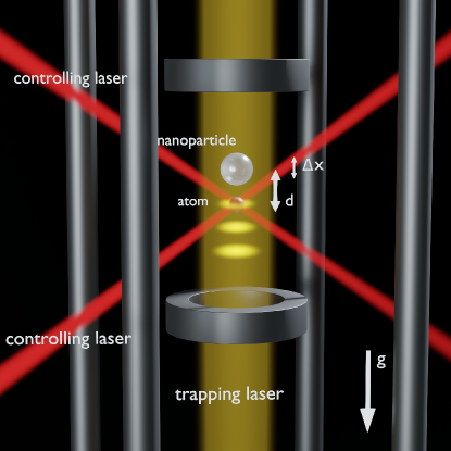
Figure 1: Scheme of the experimental setup. A nanoparticle of mass $m_{n}$ is trapped in the Paul trap. A plane wave optical field illuminates the nanoparticle and the backscatter interferes to create an intnesity maxima at distance $d$ below the nanoparticle, where we trap an atom. For a very stiff atomic trap we obtain an effective coupling between the internal state of the atom and the nanoparticle. The initial height of the nanoparticle in the trap can be controlled by changing the power of the trapping laser, which can be switched off quickly, together with softening the Paul trap to very low frequencies, approximately obtaining a free fall regime for a time $\Delta t$. We create and control the spatial superposition of the nanoparticle using additional lasers coupled to hyperfine transitions, labelled as controlling lasers, with the superposition size denoted by $\Delta x$. At the end we perform a readout of the accumulated gravitational phase $\phi_{\text{grav}}\sim m_{n}g\Delta x\Delta t/\hbar$ using a cycling transition of the internal state, where $g$ is the Earth’s gravitational acceleration.

Atom-nanoparticle coupling.— The experimental setup consists of a nanoparticle trapped in Paul trap which is illuminated by a plane-wave optical field (see Fig. 1). We choose the light wavelength $\lambda_{l}$ to be comparable or smaller than the nanoparticle radius $r$, effectively making the nanoparticle a mirror-like object. The backscattered light from the nanoparticle interferes with the incoming light to form a standing wave in the rest frame of the nanoparticle (see Fig. 2) and the resulting intensity minima and maxima rigidly follow the motion of the nanoparticle. In one of the maxima we trap an atom exploiting an internal electronic transition in the red-detuned regime. Specifically, the potential is given by:

$$\hat{H}_{\text{trap}}=\frac{m_{n}\omega_{n}^{2}}{2}\hat{x}_{n}^{2}+\frac{m_{a}\omega_{a}^{2}}{2}\left[\hat{x}_{a}-(\hat{x}_{n}+d)\right]^{2},$$ (1)

where $\omega_{n}$ ($\omega_{a}$) is the frequency of the Paul (atomic) trap, $m_{n}$ ($m_{a}$) is the mass of the nanoparticle (atom), $\hat{x}_{n}$ ($\hat{x}_{a}$) is the nanoparticle (atom) position, and $d$ is the distance between the two traps.

The motional frequency of the atom is given by (grimm2000optical, ):

$$\omega_{a}=\sqrt{\frac{6\pi c^{2}}{m_{a}w^{2}\text{$\omega_{e}^{3}$}}I\frac{\Gamma}{\Delta}},$$ (2)

where $I$ is the intensity of light at the trap center, $w\sim\lambda_{l}/2$ is the trap width, $\omega_{e}$ is the electronic transition frequency, $\Gamma$ is the decay rate from the excited state, $\Delta=\omega_{e}-\omega_{l}$ is the detuning of the light field, $\omega_{l}=\frac{2\pi c}{\lambda_{l}}$, and $c$ is the speed of light. To obtain high trapping frequencies we can decrease the detuning $\Delta$ at the cost of reducing the trapping time $\tau_{\text{trap}}=\frac{m_{a}c^{2}}{\hbar\text{$\omega_{l}$}^{2}}\frac{\Delta}{\Gamma}$.

The trapped atom offers a new handle on motion of the nanoparticle. Particularity interesting is the situation when the atom is placed in a strong dipole trap, resulting in a rigid atom-nanoparticle coupling. We then expect that any displacement of the atom will drag the whole atom-nanoparticle system, with only negligible excitation of the relative motion between the two. Mathematically, this translates to requiring that (i) the atom is placed in the motional ground state and (ii) the zero-point motion of the atom, $\delta_{a}$, is small with respect to the one of the nanoparticle, $\delta_{n}$, such that when the nanoparticle is excited the atom remains in the ground state, i.e. we can write $\hat{x}_{a}\approx\hat{x}_{n}-d$.

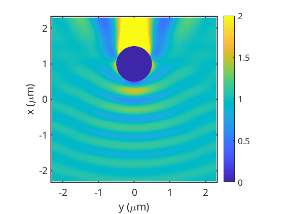
Figure 2: Simulated intensity using finite difference time domain methods (sim1, ; lumerical, ). We consider a nanoparticle of radius $r=500$nm and an optical field with wavelength $\lambda_{l}=1000$nm propagating in the posive $x$-axis direction. The incoming field is polarized along the $y$-axis; other vertical planes shows a similar intensity profile. The colour bar is the enhancement in the square of the electric field. The large blue circle denotes the nanoparticle; the incoming field propagating from the bottom interferes with the backcattered field from the nanoparticle which creates dipole traps below the nanoparticle. The strongest dipole trap is located $d\sim 0.75\text{$\mu$m}$ below the center of the nanoparticle (first yellow patch below the blue circle).

Nanoparticle motion control.— In the considered regime we find the following interaction Hamiltonian between the motional state of the nanoparticle and the atomic hyperfine transition (in interaction picture)

$$\frac{\hat{H}_{\text{int}}}{\hbar}= \frac{\Omega_{jk}}{2}\sigma_{+}\>\text{exp}\left(i\left[\eta(\hat{a}e^{-i\omega_{n}t}+\hat{a}^{\dagger}e^{-i\omega_{n}t})-\delta t+\phi\right]\right)$$

$$+\text{H.c},$$ (3)

where we have introduced the nanoparticle mode $\hat{a}$, i.e. $\hat{x}_{n}=\delta_{n}(\hat{a}^{\dagger}+\hat{a})$. $\Omega_{jk}$ is the coupling of the stimulated Raman transition between the hyperfine states $|j\rangle$ and $|k\rangle$, $\sigma_{+}=|k\rangle\langle j|$, $\eta=k\delta_{n}$ is the Lamb-Dicke parameter, $k=\frac{2\pi}{\lambda}=\frac{\omega}{c}$ with $\omega$ the frequency of the laser, $\delta=\omega_{h}-\omega$ is the detuning that selects one of the sidebands or the carrier resonance, $\omega_{h}$ is the hyperfine transition frequency, and $\phi$ is a phase that includes $\frac{d}{\lambda}$. Here we limit the discussion to $\eta\ll 1$, which puts a lower bound on the Paul trap frequency, i.e. $\frac{\hbar}{2m_{n}\lambda^{2}}\ll\omega_{n}$. The coupling of the stimulated Raman transition is given by $\Omega_{jk}\equiv g_{jk}$, where $g_{jk}=\frac{qE}{\hbar}D_{jk},$ $q$ is the electron charge, $E$ is the amplitude of the electric field, and $D_{jk}$ is the transition dipole matrix element between the state $j$ and $k$.

We are interested in two types of interactions, one that (a) controls the internal state without affecting the motional state, and one that (b) displaces the motional state without changing the internal one, both of which can be implemented in a $\Lambda$-type scheme using two lasers. In particular, using two-photon stimulated Raman transitions of type (a) and (b) we will consider three types of operations, where the coupling will be given by $\Omega_{jk}\equiv\frac{g_{jl}^{*}g_{lk}}{\Delta_{l}}$, and $\Delta_{l}$ is the detuning from the intermediate state $l$ (wineland1998experimental, ). To create a superposition of the hyperfine states we consider the carrier frequency, i.e. $\delta=0$, with a pulse of duration $t=\pi/(2\Omega_{\uparrow\downarrow})$ using scheme (a), namely a $\pi/2$ pulse. This generates a beam splitter transformation, i.e. the hyperfine states evolve in the following way: $|\uparrow\rangle\rightarrow(|\uparrow\rangle-|\downarrow\rangle)/\sqrt{2}$ and $|\downarrow\rangle\rightarrow(|\uparrow\rangle+|\downarrow\rangle)/\sqrt{2}$. Similarly, a $\pi$ pulse using scheme (a) at the carrier corresponds to $\Omega_{\uparrow\downarrow}t=\pi$ and $\delta=0$, which exchanges the hyperfine states, i.e. $|\uparrow\rangle\rightarrow-|\downarrow\rangle$ and $|\downarrow\rangle\rightarrow|\uparrow\rangle$. On the other hand, to displace the motional state without modifying the hyperfine state we exploit scheme (b) at the first red sideband, i.e $\delta=\omega_{n}$. This latter operation produces a displacement of the motional state by $\Omega_{\downarrow\downarrow}\eta t$, where $t$ is the duration of the pulse.

In summary, the discussed interactions have the same form as the ones exploited in atomic physics where in place of the motional state of the atom we have the motional state of the nanoparticle. We can thus adopt the experimentally well-established protocols from atomic physics to the nanoscale (monroe1996schrodinger, ; itano1997quantum, ; wineland1998experimental, ).

Schrödinger’s cat.— Suppose the state of the system is $|\Psi\rangle=|\psi\rangle_{h}|\psi\rangle_{n}$, where $|\psi_{h}\rangle$ is the hyperfine state of the atom, and $|\psi\rangle_{n}$ is the motional state of the nanoparticle. Ideally, one would like to prepare a state of the form $|\psi\rangle_{n}\sim|\downarrow\rangle_{h}|\alpha_{\text{\text{top}}}\rangle_{n}+|\uparrow\rangle_{h}|\alpha_{\text{bottom}}\rangle_{n},$ where $|\alpha_{\text{\text{top}}}\rangle_{n}$ and $|\alpha_{\text{bottom}}\rangle_{n}$ denote states located at different heights in the Paul trap, i.e. a Schrödinger-cat state. Once such a state has been created we then want to ascertain its existence using as the readout the hyperfine state $|\psi_{h}\rangle$.

A possible strategy is to cool the system to the ground state, i.e. $|\Psi_{\text{init}}\rangle=|\downarrow\rangle_{h}|0\rangle_{n}$, and to apply the procedure described by Monroe et al (monroe1996schrodinger, ), which consists of $\pi/2$, $\pi$, and displacement pulses. To make such a scheme work one would however need additional optical fields to control the motional state of the nanoparticle. In particular, cooling to the motional ground state can be achieved with a cavity-tweezer setup (delic2019motional, ) and is expected to be soon available also in a tweezer setup (hebestreit2018sensing, ; tebbenjohanns2020motional, ).

However, a protocol that would not require cooling (ranjit2015cold, ), but would rather work for a generic trapped state, such as the experimentally more readily available thermal state, is still desirable. A second attractive feature would be to have a reliable method to evidence that the nanoscale superposition has really been probed, for example, by relating the outcome of the experiment to one of its intrinsic properties such as the nanoparticle mass $m_{n}$. A possible strategy to address both of these requirements has been outlined in (scala2013matter, ), parts of which we now adapt to the hybrid atom-nanoparticle system. For simplicity of presentation we first consider the initial state $|\psi_{\text{init}}\rangle=|\alpha\rangle\otimes|\downarrow\rangle$, where the nanoparticle is prepared in the coherent state $|\alpha\rangle$ (but we show below that it applies for any initial state). The protocol consists of the following steps.

1. Trap a nanoparticle in the Paul trap at frequency $\omega_{1}$. Trap an atom in an intensity maxima below the nanoparticle using a plane wave and cool it to the ground state using resolved sideband cooling (wineland1998experimental, ).

2. Apply a $\pi/2$ pulse to generate the state $|\psi\rangle\sim|\alpha\rangle\otimes\left(|\downarrow\rangle+|\uparrow\rangle\right)$.

3. Soften the Paul trap to frequency $\omega_{n}=\omega_{2}\ll\omega_{1}$.

4. Apply a displacement beam for a time $\delta t$ to produce the state $|\psi\rangle\sim\left(|\alpha+\beta\rangle\otimes|\downarrow\rangle+|\alpha\rangle\otimes|\uparrow\rangle\right)$, where $\beta=\Omega_{gg}\eta\delta t$.

5. Reduce the trapping laser power such that the radiation pressure force becomes small and the nanoparticle-atom system starts falling towards the Earth (matter-wave coherence is thus shielded from the deleterious effects of the laser photons and the system becomes a matter-wave sensor for the local Earth’s gravitational acceleration $\sim g$).

6. Leave the system in free fall for a time $\Delta t$ such the gravitational field induces the phase $\phi_{\text{grav}}$: $|\psi\rangle\sim\left(e^{-i\phi_{\text{grav}}}|\alpha^{\prime}+\beta\rangle\otimes|\downarrow\rangle+|\alpha^{\prime}\rangle\otimes|\uparrow\rangle\right)$, where $|\alpha^{\prime}\rangle$ is the time-evolved coherent state of $|\alpha\rangle$ .

7. Increase the trapping laser power back to its initial value. Apply a displacement beam for a time $\delta t$ to reverse the effect of step 4 and obtain a factorizable state $|\psi\rangle\sim|\alpha^{\prime}\rangle\otimes\left(e^{-i\phi_{\text{grav}}}|\downarrow\rangle+|\uparrow\rangle\right)$.

8. Apply a $\pi/2$ pulse to create the final state $|\psi\rangle\sim|\alpha^{\prime}\rangle\otimes|\phi\rangle$, where the hyperfine state is $|\phi\rangle=\text{cos }\left(\frac{\phi_{\text{grav}}}{2}\right)|\downarrow\rangle-\text{sin}\left(\frac{\phi_{\text{grav}}}{2}\right)|\uparrow\rangle.$

9. Apply a laser field to drive a cycling transition and find the probability of being in the ground state $P_{\downarrow}=\text{cos}^{2}\left(\frac{\phi_{\text{grav}}}{2}\right)$.

10. After the measurement we recapture the nanoparticle by modulating the radiation pressure from the trapping laser and the Paul trap frequency.

The induced gravitational phase difference is given by

$$\phi_{\text{grav}}=\frac{m_{n}g\Delta x\Delta t}{\hbar},$$ (4)

where $\Delta x=\delta_{n}\beta=\frac{\hbar k}{2m_{n}\omega_{2}}\Omega_{gg}\delta t$ is the superposition size of the nanoparticle and $\Delta t$ is the duration of the transient free fall motion. Since the nanoparticle mass $m_{n}$ is large we can have $\phi_{\text{grav}}\sim 1$ already for small superposition sizes $\Delta x$ and for short free-fall times $\Delta t$ – a regime which is interesting on its own.

Let us now consider a generic initial state $\rho_{\text{init}}=\rho_{n}\otimes|\downarrow\rangle\langle\downarrow|$, where $\rho_{\text{\text{n}}}=\int d^{2}\alpha P_{n}(\alpha)|\alpha\rangle\langle\alpha|,$ and $P$ is Glauber’s P quasi-probability distribution. Here we only require that the nanoparticle is initially trapped in the Paul trap, but the motional state can be otherwise completely generic. The steps 1-7 now result in the final state $\rho_{\text{final}}\sim\rho^{\prime}_{n}\otimes|\phi\rangle\langle\phi|$, where $\rho^{\prime}_{n}$ is the final motional state of the nanoparticle, yet $|\phi\rangle$ is the same internal state obtained by considering an initial coherent motional state. Remarkably, the transient free fall dynamics entangles the motional and internal states in a simple way which can be readily disentangled at any time — this is a direct consequence of the uniform nature of the universal gravitational coupling, a feature which is absent already with a harmonic potential. Creating a superposition of an arbitrary motional state (such as of a thermal state) still fully retains its coherent properties, and once the gravitational phase is transferred to the internal state it can be then read out again using steps 8 an 9.

Discussion.— We can estimate the requirements to achieve $\phi_{\text{grav}}\sim 1$ for a typical tabletop experiment using a nanoparticle of radius $r=500\text{nm}$ and mass $m_{n}\sim 10^{-15}\text{kg}$ in a Paul trap (bullier2020characterisation, ; pontin2019ultranarrow, ). As discussed, we first trap an atom in a dipole trap near the nanoparticle, which induces a coupling between the two, while other interactions between the atom and the charged nanoparticle are negligible. For concreteness we consider a Cs atom and the $D_{2}$ transition $6^{2}S_{\frac{1}{2}}\rightarrow 6^{2}P_{\frac{3}{2}}$ which has a transition dipole matrix element $\sim 4\times 10^{-29}\text{Cm}$ and decay rate $\Gamma\sim 3\times 10^{7}\text{Hz}$.

We set the detuning of the trapping laser to $\Delta\sim 5\times 10^{11}\text{Hz}$ to generate a far red-detuned dipole trap: we find a trap lifetime $\tau_{\text{trap}}\sim 1\text{s}\gg\Delta t$ and using Fig. 2 we estimate the atomic trap frequency to be $\omega_{a}\sim 5\times 10^{6}\text{Hz}$ generated by an incoming (backscattered) intensity $\sim 5\times 10^{12}\text{Wm}^{-2}$($\sim 3\times 10^{7}\text{Wm}^{-2}$). Such an intensity can be obtained using an unfocused laser beam at moderate power; at this intensity the radiation pressure force cancels the gravitational one (whilst not co-trapping the nanoparticle). We consider a short free fall-time $\Delta t\sim\omega_{a}^{-1}\sim 1\text{$\mu$s}$ in order to retain the atom’s motional state which corresponds to a displacement of $\sim 5\text{pm}$. The condition to excite the nanoparticle motion constrains the Paul trap frequency $\omega_{n}$ from above, $\omega_{n}\ll 5\times 10^{-4}\text{Hz}$, and the Lamb-Dicke condition from below, $\omega_{n}\gg 5\times 10^{-8}\text{Hz}$. Specifically, we set the initial Paul trap frequency to $\omega_{1}=0.1\text{kHz}$ which is then softened to $\omega_{2}=5\times 10^{-6}\text{Hz}$. After the Paul trap is softened we create a spatial superposition of the nanoparticle by illuminating the atom with a short laser pulse of duration $\sim 100\text{ps}$ and detuning $\Delta_{3}\sim 10^{11}\text{Hz}$. The requirement of unit phase, $\phi_{\text{grav}}\sim 1$, fixes the intensity of the beam to $I\sim 1\text{Wm}^{-2}$, resulting in a tiny nanoparticle superposition of size $\Delta x\sim 10^{-14}\text{m}$. The control beam will illuminate also the nanoparticle (given its close proximity $d\sim 0.75\mu m$), but such a tiny intensity will however not lead to any measurable dephasing. Larger as well as smaller superpositions can be created by varying the parameters of the setup, for example, by controlling the intensity and duration of the displacement beam one is expected to achieve superpositions of the size of the nanoparticle. Additionally, to further enlarge the size of the superposition –without extending the duration of the experiment – one could also introduce a boosting potential by adaptation of the coherent inflation method to the Paul trap (romero2017coherent, ).

The decoherence times for superposition sizes $\Delta x\sim 10^{-14}\text{m}$ exceed the duration of the experimental time $\Delta t\sim 1\mu s$ at readily available pressures and temperatures – for concreteness we consider the vacuum chamber with pressure $p\sim 10^{-2}\text{mbar}$ and temperature $T\sim 300\text{K}$. Given the modest laser intensities, and the relatively high pressure, we can assume that both the center-of-mass and internal temperature of the nanoparticle remain below $T\sim 1000\text{K}$ (hebestreit2018measuring, ) (for cooling the internal temperature see (rahman2017laser, )). At such pressures/temperatures we find that gas collisions limit the coherence time to $\sim 6\mu s$, while decoherence due to photon emission/absorption remains negligible – at $T\sim 300\text{K}$ the available coherence time is further extended (schlosshauer2007decoherence, ; romero2011quantum, ; seberson2019distribution, ).

For completeness we also estimate the emitted thermal radiation from the nanoparticle and its effect on the atom. Assuming black-body radiation from the nanoparticle with internal temperature $T\sim 1000\text{K}$ we find a radiated intensity $\sim 10^{5}\text{Wm}^{-2}$ which is two orders below the intensity generating the atom’s dipole trap (see above). Furthermore, the intensity of the thermal radiation in the narrow frequency range of the internal transition Cs $D_{2}$($6^{2}S_{\frac{1}{2}}\rightarrow 6^{2}P_{\frac{3}{2}}$) is $\sim 10^{-6}\text{Wm}^{-2}$ which has to be compared with the intensity of the controlling lasers $\sim 1\text{Wm}^{-2}$. We have to however re-scale the two intensities by the ratio of the duration of the experiment ($\sim 1\text{\leavevmode{m}s}$ and of the controlling pulse and $\sim 100\text{ps}$) which nonetheless still results in the coherent laser radiation dominating by 2 orders of magnitude over the thermal one. If instead one assumes an internal temperature $T\sim 300\text{K}$ the effect of thermal radiation becomes dwarfed by the controlling beams by about $\sim 20$ orders of magnitude and can thus be again neglected.

Finally, we estimate the effect of voltage noise, $S_{V}$, which gives rise to a force noise, $S_{f}^{\text{(vol)}}\sim qS_{V}/D$, where $q$ is the net charge on the nanoparticle, and $D$ is a characteristic distance to the electrodes. Specifically, assuming $S_{V}\sim 10\text{$\mu$V}/\text{Hz}^{1/2}$, $q\sim 80e$ (we note that the charge on the nanoparticle can be controlled to a high degree (bullier2020characterisation, )), and $D\sim\text{2.3\text{mm}}$ we find $S_{f}^{\text{(vol)}}\sim 10^{-23}\text{N}/\text{Hz}^{1/2}$(pontin2019ultranarrow, ). By comparison the force noise due to gas collisions is $S_{f}^{\text{(gas)}}\sim\sqrt{2k_{b}Tm_{n}\gamma}$, where $\gamma=4\pi m_{g}r^{2}v_{t}p/(3k_{b}Tm_{n})(1+\pi/8)$ is the gas damping rate (epstein1924resistance, ; cavalleri2010gas, ), $m_{g}$ is the molecular mass, and $v_{t}=\sqrt{8k_{b}T/(\pi m_{n})}$ is the thermal gas velocity – using $T\sim 300\text{K}$ and $p\sim 10^{-2}\text{mbar}$ we find $S_{f}^{\text{(gas)}}\sim 10^{-16}\text{N}/\text{Hz}^{1/2}$. As discussed above the thermal noise does not impede the witnessing of interference and hence voltage noise can be also safely neglected.

The insensitivity of the ten-step protocol to the environment can be explained by the fact that the characteristic wavelength of gas particles as well as the ones associated with laser and environmental photons, is much larger than $\Delta x$, making the associated decoherence times long compared to the short free fall time.

In summary, we have shown that it is possible to create motional superposition of massive objects (a $\sim 500$nm radius nano-object) by introducing a coupled atom-nanoparticle hybrid system and discussed how to detect them. It will extend the demostration of the superposition principle to unprecedented regimes of mass, $10^{8}$ times the current record (fein2019quantum, ). The method has several appealing features. It works for a generic initial state, the control and readout of the motional state is through well established versatile atomic protocols, and the created superposition is very well protected from deleterious decoherence effects.

Acknowledgements.— We acknowledge support from EPSRC grant EP/N031105/1. MT acknowledges funding by the Leverhulme Trust (RPG-2020-197).

Appendix A Atom-Nanoparticle motion and internal transitions

We discuss the center-of-mass variables (Sec. A), which allows to reduce the problem to the effective interaction between the motional state of the nanoparticle (Sec. B) and the internal hyperfine state of the atom (Sec. C).

A.1 Center-of-mass motion

We introduce the center-of-mass (c.o.m.) variables

$$\hat{R} =\frac{m_{n}\hat{x}_{n}+m_{a}\hat{x}_{a}}{m_{n}+m_{a}},\qquad\hat{r}=\hat{x}_{n}-\hat{x}_{a},$$ (5)

where $\hat{R}$ ($\hat{r}$) is the c.o.m. (relative) position. The corresponding zero-point motions are given by $\delta_{n}=\sqrt{\frac{\hbar}{2M\omega_{n}}}$ and $\delta_{a}=\sqrt{\frac{\hbar}{2\mu\omega_{a}}}$ , where we have introduced the total mass $M=m_{n}+m_{a}\sim m_{n}$ and the reduced mass $\mu=\frac{m_{a}m_{n}}{M}\sim m_{a}$. We define the mechanical modes as

$$\hat{R}=\delta_{n}(\hat{a}+\hat{a}^{\dagger})\qquad\hat{r}-d=\delta_{a}(\hat{b}+\hat{b}^{\dagger}),$$ (6)

and using Eq. (1) we readily find the nanoparticle-atom Hamiltonian:

$$H_{\text{nano-atom}}=\hbar\omega_{n}\hat{a}^{\dagger}\hat{a}+\hbar\omega_{a}\hat{b}^{\dagger}\hat{b}.$$ (7)

We will be primarily interested in controlling the c.o.m. mode $\hat{a}$ which to good approximation coincides with the motion of the nanoparticle. We consider the rigid-coupling regime discussed in the main text, i.e. we prepare the atom in the motional ground state and require $\delta_{n}\gg\delta_{a}$. More specifically, we require that the displacement beam will not excite the atom’s motional state, while sufficiently exciting the nanoparticle.

Some remarks about the approximations involved are in order. In Eq. (7) we have neglected terms of order $\sim\mathcal{O}(m_{a}/m_{n})$ which for typical atomic and nanoscale masses would correspond to a correction of $1$ part in $\sim 10^{8}$. The analysis was also based on a semiclassical approximation, where the internal motion responsible for the atomic polarizability is assumed to reach a steady-state on a time-scale faster than the motional time-scale of the atom in the trap GRIMM200095 . The full dynamics would require simultaneous integration of the optical Bloch equations together with the atom-nanoparticle motional dynamics as described by the quantum kinetic equations balykin2000electromagnetic ; leibfried2003quantum ; chang2002density . In the following we will also consider additional lasers for controlling the motional state of the atom; we will suppose that the atom remains stably trapped for the duration of the experiment garraway2000theory ; jun2001stability .

A.2 Nanoparticle potential

The potential of the nanoparticle in the Paul trap is given by

$$\hat{H}_{\text{nano}}=\frac{m_{n}\omega_{n}^{2}}{2}\hat{x}_{n}^{2}+m_{n}g_{E}\hat{x}_{n}-F\hat{x}_{n},$$ (8)

where we have introduced the gravitational force $m_{n}g_{E}$ as well as the radiation pressure force $F$ generated by the trapping laser for the atom (see Fig. 1).

We first trap the nanoparticle in a relatively stiff Paul trap $\omega_{n}=\omega_{1}$ with the radiation pressure force $F$ constrained by the requirement of stable trapping in the Paul trap. The latter is controlled by light intensity $I$ which also sets the atomic trap frequncy $\omega_{a}$ in Eq. (2). Given the large mass of the nanoparticle in comparison with the atom’s mass we can have both a small radiation pressure force $F\sim m_{n}g_{E}$ as well as a high trapping frequency $\omega_{a}$ for the atom – the latter is required to introduce a handle on the nanoparticle’s motion.

We then release the nanoparticle by (i) softening the Paul trap frequency from $\omega_{n}=\omega_{1}$ to $\omega_{n}=\omega_{2}$ as well as (ii) reducing the radiation pressure such that $F\ll m_{n}g_{E}$. The net result is a change of equilibrium position and for a transient period the nanoparticle is in free fall evolving according to the potential

$$\hat{H}_{\text{nano}}\approx m_{n}g_{E}\hat{x}_{n}.$$ (9)

In a nutshell, the idea is to suddenly release the nanoparticle from the trap and use laser fields to create a spatial superposition exploiting the atom-nanopaticle coupling. We effectively create a Mach-Zehnder type interferometer for the nanoparticle: we exploit the Earth’s gravitational acceleration $\sim g_{E}$ to impart a phase difference on the spatial parts of the superposition, which is then transferred to the internal state and read out.

A.3 Two-photon stimulated Raman transitions

We consider two types of interactions, one that (a) controls the internal state without affecting the motional state, and one that (b) displaces the motional state of the nanoparticle without changing the internal one wineland1998experimental .

In the former case (a) one links the ground and excited hyperfine states, i.e. the states $|\uparrow\rangle$ and $|\downarrow\rangle$, respectively, through a third hyperfine state $|3\rangle$ using lasers of frequencies $\omega_{1}$ and $\omega_{2}$: on resonance we would have $|\omega_{1}-\omega_{2}-\Delta_{3}|=\omega_{h}$ with $\Delta_{3}$ a suitably chosen detuning from the state $|3\rangle$. Furthermore, we assume that the corresponding wave-vectors, $\bm{k}_{1}$ and $\bm{k}_{2}$, are such that their difference $\delta\bm{k}=\bm{k}_{1}-\bm{k}_{2}$ is parallel to the vertical $x$-axis with the projection denoted by $\delta k$. Formally the interaction Hamiltonian is again given by Eq. (3), where $\eta=\delta k\delta_{n}$, and the coupling is given by $\Omega_{\uparrow\downarrow}\equiv\frac{g_{\uparrow 3}^{*}g_{3\downarrow}}{\Delta_{3}}$. If we work at the carrier frequency, i.e. $\delta t=0$, the dominant term in the Hamiltonian is insensitive to $\delta k$ and the motional state remains unaffected, i.e. we only change the hyperfine state. In the latter case (b) one instead stimulates the transitions $|\downarrow\rangle\rightarrow|3\rangle$ and $|3\rangle\rightarrow|\downarrow\rangle$, resulting in a coupling $\Omega_{\downarrow\downarrow}\equiv\frac{g_{\downarrow 3}^{*}g_{3\downarrow}}{\Delta_{3}}$. Here we want to induce big displacements of the nanoparticle for which large values of $\delta k$ are preferrable, e.g. $\delta k\sim|\bm{k}_{1}|$,$|\bm{k}_{2}|$. The Hamiltonian is still the one in Eq. (3) with the formal replacement $\sigma_{+}\rightarrow\mathbb{I}$, where $\mathbb{I}$ is the identity matrix: now the hyperfine state is unaffected and the motional state changes, i.e. a displacement beam.

Appendix B Classical evolution

We consider the motion of a point particle of mass $m$ in a harmonic trap with frequency $\omega$ in the Earth’s gravitational field. In particular, the total Hamiltonian of the problem is given by

$$H_{1} =\frac{p_{1}^{2}}{2m}+\frac{1}{2}m\omega^{2}x_{1}^{2}+mg_{E}x_{1},$$ (10)

where $x_{1}$ ($p_{1}$) denote the position and momentum observable, and $g_{E}$ is the gravitational acceleration. Here we will denote the Earth’s gravitational acceleration by $g_{E}$ while reserving the symbol $g$ for the corresponding coupling which depends on $\omega_{n}$ (see Eq. 21). In Eq. (10) the subscript $1$ labels the reference frame. We also introduce a shifted reference, i.e. reference frame $2$, where the positions and momenta are given by

$$x_{2}=x_{1}+\frac{g_{E}}{\omega^{2}},\qquad p_{2}=p_{1},$$ (11)

and the Hamiltonian is

$$H_{2}=\frac{p_{2}^{2}}{2m}+\frac{1}{2}m\omega^{2}x_{2}^{2}.$$ (12)

We are ultimately interested in the evolution described in reference frame $1$, i.e. the evolution arising from Eq. (10). However, as we will see when discussing the quantum case, it is instructive to compare it to description in the shifted reference frame 2, i.e. the evolution arising from Eq. (12). Specifically, in reference 2 we find the solution to be a simple harmonic motion:

$$x_{2} =x_{2}(0)\text{cos}(\omega t)+\frac{p_{2}(0)}{m\omega}\text{sin}(\omega t),$$ (13)

$$p_{2} =-m\omega x_{2}(0)\text{sin}(\omega t)+p_{2}(0)\text{cos}(\omega t).$$ (14)

Using Eq. (11) we then immediately find the solution in reference frame 1:

$$x_{1}= x_{1}(0)\text{cos}(\omega t)+\frac{p_{1}(0)}{m\omega}\text{sin}(\omega t)$$

$$+\frac{g_{E}}{\omega^{2}}(\text{cos}(\omega t)-1),$$ (15)

$$p_{1}= -m\omega x_{1}(0)\text{sin}(\omega t)+p_{1}(0)\text{cos}(\omega t)$$

$$-m\omega\frac{g_{E}}{\omega^{2}}\text{sin}(\omega t).$$ (16)

We now consider two different limits. We note that by taking the limit $g_{E}\rightarrow 0$ we recover simple harmonic motion, for example the whole experiment, including the trap, is in free fall, i.e. we recover Eqs. (13) and (14) with the formal replacement $x_{2}\rightarrow x_{1}$, $p_{2}\rightarrow p_{1}$. On the other hand, in the limit $\omega\rightarrow 0$, i.e. we switch off the trap, we find:

$$x_{1} =x_{1}(0)+\frac{p_{1}(0)}{m}t-\frac{g_{E}t^{2}}{2},$$ (17)

$$p_{1} =p_{1}(0)-mg_{E}t,$$ (18)

as expected for free fall.

To relate the results to a quantum analysis we introduce the zero-point motions, $\delta_{x}=\sqrt{\frac{\hbar}{2m\omega}}$ and $\delta_{p}=\sqrt{\frac{\hbar m\omega}{2}}$, and the adimensional position and momentum,

$$X_{1} =\frac{x_{1}}{\delta_{x}}=a+a^{*},\qquad P_{1}=\frac{p_{1}}{\delta_{p}}=i(a^{*}-a).$$ (19)

The gravitational potential becomes

$$U=\hbar gX_{1},$$ (20)

where the gravitational coupling is

$$g=g_{E}\sqrt{\frac{m}{2\hbar\omega}}.$$ (21)

The transition from harmonic to free fall motion depends on the strength of the frequencies $\omega$ and $g$, which we now explore. We rewrite Eqs. (15) and (16) using Eqs. (19):

$$X_{1}= X_{1}(0)\text{cos}(\omega t)+P_{1}(0)\text{sin}(\omega t),$$

$$+2\frac{g}{\omega}(\text{cos}(\omega t)-1)$$ (22)

$$P_{1}= -X_{1}(0)\text{sin}(\omega t)+P_{1}(0)\text{cos}(\omega t)$$

$$-2\frac{g}{\omega}\text{sin}(\omega t).$$ (23)

Taking the limit $g\rightarrow 0$ amounts to vanishing third terms on the righthand side in Eqs. (22) and (23), which is the expected result as discussed above. On the other hand, naively taking the limit $\omega\rightarrow 0$ in Eqs. (22) and (23) does not give the free fall evolution: the reason is that these have been derived from Eqs. (22) and (23) by diving/mupltipliying with $\delta_{x}$ and $\delta_{p}$ which depend on the harmonic frequenciy $\omega$. A similar problem is encountered also by using the modes

$$a_{1}=\frac{X_{1}+iP_{1}}{2},\qquad a_{1}^{*}=\frac{X_{1}-iP_{1}}{2}.$$ (24)

Specifically, from Eqs. (22) and (23) we find:

$$a_{1}= a_{1}(0)e^{-i\omega t}+\frac{g}{\omega}(e^{-i\omega t}-1),$$ (25)

where we are again confronted on how to consider the limiting free-fall case.

The problem of taking the limit $\omega\rightarrow 0$ can be avoided by considering small adimensional expansion parameters, $gt$ and $\omega t$ – to study the free-fall case, we choose to expand to quadratic order. Following the latter procedure we find from Eq. (25):

$$a_{1}\approx a_{1}(0)\left[1-i\omega t-\frac{1}{2}\omega^{2}t^{2})\right]+igt-\omega\frac{gt^{2}}{2}.$$ (26)

If we move back to the position-momentum description we find:

$$x_{1}= x_{1}(0)+\frac{p_{1}(0)}{m}t+x_{1}(0)\frac{\omega^{2}t^{2}}{2}-\frac{g_{E}t^{2}}{2},$$ (27)

$$p_{1}= p_{1}(0)-m\omega^{2}x_{1}(0)t+p_{1}(0)\frac{\omega^{2}t^{2}}{2}-mg_{E}t.$$ (28)

Eqs. (27) and (28) have extra $\omega$-dependent terms which were absent in the $\omega\rightarrow 0$ limit (see Eqs. (17) and (18)). Unlike the former $\omega\rightarrow 0$ calculation, the approximation procedure is not state-independent, but depends on the value of $x_{1}(0)$ and $p_{1}(0)$. In order to recover exactly free-fall one is implicitly assuming that the initial position and momentum, $x_{1}(0)$ and $p_{1}(0)$, are small enough when taking the $\omega\rightarrow 0$ limit.

However, as we will explicitly see in the next sections we can retain the additional $\omega$-dependent terms as they do not change the induced gravitational phase – as long as $\omega t$ remains small. Furthermore, higher order harmonic terms – beyond the free fall approximation – are interesting on its own and could be used to ascertain the spatial superposition of large nanoparticles without resorting to a dynamical equilibrium change (see section E).

Appendix C Quantum evolution

In this section we consider the quantum dynamics of a particle of mass $m$ harmonically trapped and subject to the Earth’s gravitational potential. We continue to use the notation of Sec. B where the observables, e.g. $O$, are promoted to operators, e.g. $O\rightarrow\hat{O}$. The classical analysis of the transition from harmonic to free fall motion –in particualr the approximations involved – carry over also to the quantum case. To simplify the notation we will omit the subscript $1$ for quantities related to reference frame $1$ most of the time.

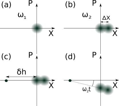
Figure 3: We consider the vertical motion of a particle in a Paul trap in an Earth-bound laboratory. (a) The nanoparticle is initially confined in a trap with frequency $\omega_{1}$ and kept close to the origin of the trap; the gravitational force $mg_{E}$, where $m$ is the mass of the nanoparticle and $g_{E}$ is the gravitational acceleration, is counter-balanced by a radiation pressure force. (b) We change the frequency to $\omega_{2}\ll\omega_{1}$ and create a small superposition of size $\Delta x=\sqrt{\frac{\hbar}{2m\omega_{2}}}\Delta X.$ (c) We decrease the radiation pressure force making it negligible with respect to the gravitational one; this changes the equilibrium position to $g_{E}/\omega_{2}^{2}=\sqrt{\frac{\hbar}{2m\omega_{2}}}\delta h$. (d) We let the system evolve for a short time $t$ such that the motion of the particle is governed by the uniform gravitational field. This transient free fall regime can be understood graphically – we note that the small arc drawn at radius $\delta h$ with subtended angle $\omega_{2}t$ can be well approximated by the initial part of a parabolic curve.

C.1 Change of equilibrium

We consider the operator version of the Hamiltonian in Eqs. (10) which we rewrite as

$$\hat{H} =\hbar\omega\hat{a}^{\dagger}\hat{a}+\hbar g(\hat{a}^{\dagger}+\hat{a}),$$ (29)

and an initial coherent state $|\alpha\rangle$ associated to the $\hat{a}$ mode.

We first recall the definition of the displacement operator:

$$\hat{D}(\alpha)=e^{\alpha\hat{a}^{\dagger}-\alpha^{*}\hat{a}},$$ (30)

and the multiplication rule

$$\hat{D}(\alpha)\hat{D}(\beta)=e^{\frac{1}{2}(\alpha\beta^{*}-\alpha^{*}\beta)}\hat{D}(\alpha+\beta).$$ (31)

To find the time-evolution we restate the problem in a displaced frame:

$$|\alpha\rangle \overset{\hat{D}}{\rightarrow}|\chi\rangle_{2}=\hat{D}(\delta)|\alpha\rangle,$$ (32)

$$\hat{H} \overset{\hat{D}}{\rightarrow}\hat{H}_{2}=\hat{D}(\delta)\hat{H}\hat{D}(\delta\alpha)^{\dagger},$$ (33)

where $\delta\equiv\frac{g}{\omega}$. In particular, we find $\hat{H}_{2}=\hbar\omega\hat{a}^{\dagger}\hat{a}$ and using Eqs.(30)-(31) we find the time evolved state

$$|\chi\rangle_{2}\rightarrow|\chi_{t}\rangle_{2}=e^{\frac{g}{2\omega}(\alpha^{*}-\alpha)}|(\alpha+\frac{g}{\omega})e^{-i\omega t}\rangle.$$ (34)

We now go back to the original frame using the inverse transformation

$$|\chi_{t}\rangle_{2} \overset{\hat{D}^{\dagger}}{\rightarrow}\hat{D}^{\dagger}(\delta)|\chi_{t}\rangle_{2}$$ (35)

Using again Eqs. (30) and (31) we finally find the time evolution of the state in the original frame:

$$|\alpha\rangle\rightarrow e^{\frac{g}{2\omega}\left[\alpha^{*}(1-e^{i\omega t})-\alpha(1-e^{-i\omega t})\right]}|\alpha e^{-i\omega t}+\frac{g}{\omega}(e^{-i\omega t}-1)\rangle,$$ (36)

We expand to order $\mathcal{O}(t^{2})$ analogously as in the classical case:

$$|\alpha\rangle\rightarrow e^{-\frac{i}{2}(\alpha^{*}+\alpha)gt}e^{\frac{1}{2}(\alpha^{*}-\alpha)\omega\frac{gt^{2}}{2}}$$

$$|\alpha(1-i\omega t-\frac{1}{2}\omega^{2}t^{2})-igt-\frac{\omega gt^{2}}{2}\rangle,$$ (37)

where we recognize in the first and second prefactors on the righthand side a boost and a translation, respectively. In particular, using Eq. (21) the phase factors expressed become

$$-i\frac{(\alpha^{*}+\alpha)gt}{2} =-i\frac{1}{2}\frac{x}{\hbar}\frac{g_{E}t}{2}$$ (38)

$$\frac{1}{2}(\alpha^{*}-\alpha)\omega\frac{gt^{2}}{2} ==-i\frac{1}{2}\frac{p}{\hbar}\frac{g_{E}t^{2}}{2}$$ (39)

where $x=\delta_{x}(\alpha^{*}+\alpha)$ and $p=i\delta_{p}(\alpha^{*}-\alpha)$. Similary, the state of the system $|\alpha\rangle$ has now been been boosted by$-gt$ as well as displaced by $-\frac{\omega gt^{2}}{2}$ in accordance with the classical evolution in Eq. (26).

C.2 Change of equilibrium and frequency

We consider the time-dependent Hamiltonian:

$$\hat{H}(t)=\frac{\hat{p}^{2}}{2m}+\frac{m\omega(t)^{2}}{2}\hat{x}^{2}+m\omega(t)^{2}d(t)\hat{x},$$ (40)

where $\hat{x}$ and $\hat{p}$ are the operators associated to the reference frame centered at the Paul-trap origin, i.e. reference frame $1$. In particular, we have a sudden change of equilibrium position, $d(t)$, and of the Paul trap frequency, $\omega(t)$, i.e.,

$$\omega(t) =\begin{cases}\omega_{1},&t\leq 0\\ \omega_{2},&t>0\end{cases},$$ (41)

$$d(t) =\begin{cases}0,&t\leq 0\\ \frac{g_{E}}{\omega_{2}^{2}},&t>0\end{cases}.$$ (42)

For $\omega_{2}=\omega_{1}$ one finds the problem already discussed in the previous section C.1.

Here we consider the full dynamics with the Hamiltonian defined in Eqs. (40)-(42). We consider an initial coherent state $|\alpha\rangle$ associated to the mode $\hat{a}=\sqrt{\frac{\hbar}{2m\omega_{1}}}(\hat{x}+i\hat{p})$ prepeared at time $t=0$. The time-evolution for $t>0$ can be explicitly computed ma1989squeezing :

$$|\alpha\rangle\rightarrow\hat{S}(z)\hat{D}(\epsilon)\hat{R}(\phi)|\alpha\rangle,$$ (43)

where the operators are given by

$$\hat{S}(z) =e^{\frac{1}{2}(z\hat{a}^{\dagger 2}-z^{*}\hat{a}^{2})},$$ (44)

$$\hat{D}(\epsilon) =e^{\frac{1}{2}(\epsilon\hat{a}^{\dagger}-\epsilon^{*}\hat{a})},$$ (45)

$$\hat{R}(\phi) =e^{+i\phi\hat{a}^{\dagger}\hat{a}},$$ (46)

and the time-dependent parameters are defined as follows

$$e^{i\theta} \tanh|z|=\frac{(e^{-2i\omega_{2}t}-1)\tanh r}{1-e^{-2i\omega_{2}t}\tanh^{2}r},$$ (47)

$$\epsilon =\delta e^{i\phi}(1-e^{i\omega_{2}t})(\cosh r+e^{-i\omega_{2}t}\sinh r),$$ (48)

$$e^{i\phi} =\frac{1-e^{2i\omega_{2}t}\tanh^{2}r}{|1-e^{2i\omega_{2}t}\tanh^{2}r|}e^{-i\omega_{2}t}.$$ (49)

We have two squeezing parameters: the customary one is given by $r=\frac{1}{2}\text{ln}(\frac{\omega_{2}}{\omega_{1}})$ and the dynamical one by $z=|z|e^{i\theta}$. The equilibirium position in adimensional units is given by $\delta=\frac{g_{2}}{\omega_{2}}$ which is contained in the time-dependent parameter $\epsilon$, where $g_{2}=g_{E}\sqrt{\frac{m}{2\hbar\omega_{2}}}$ is the coupling induced by the gravitational acceleration.

We want to expand Eq. (43) to order $\mathcal{O}(t^{2})$ during which the system is approximately in free fall as discussed in the previous sections. However Eq. (43) is not yet in a suitable form as displacement and rotation operators preceed the squeezing one; $\hat{S}(z)$ applied on a displaced coherent state also changes its displacement. To avoid this problem we adapt the analysis from ma1989squeezing to commute the operators:

$$\hat{S}(z)\hat{D}(\xi)=\hat{D}(\gamma)\hat{S}(z)$$ (50)

where

$$\xi =\epsilon+\alpha e^{i\phi},$$ (51)

$$\gamma =\xi\cosh|z|-\xi^{*}\sinh|z|e^{i(\theta+\pi)}.$$ (52)

We can thus rewrite Eq. (43) using Eq. (31) and Eq. (50) as

$$|\alpha\rangle\rightarrow e^{\frac{1}{2}(\epsilon\alpha^{*}e^{-i\phi}+\epsilon^{*}\alpha e^{i\phi})}\hat{D}(\gamma)\hat{S}(z)|0\rangle$$ (53)

We first note that the dynamical squeezing parameter $z$ in Eq. (47) is only of order $\mathcal{O}(\omega_{1}t)$:

$$z=\frac{it\left(\text{$\omega_{1}^{2}$}-\omega_{2}^{2}\right)}{2\omega_{1}}\approx i\omega_{1}t.$$ (54)

where we have assumed $\omega_{2}\ll\omega_{1}$. Wence we can neglect squeezing and set $\hat{S}(z)\sim\mathbb{I}$ by assuming $\omega_{1}t\ll 1$ (and hence also $\omega_{2}t\ll 1$) . Performing a series expansion, keeping only the relevant terms, we obtain from Eq. (43) the following evolution:

$$|\alpha\rangle\rightarrow e^{-\frac{i}{2}(\alpha^{*}+\alpha)\sqrt{\frac{\omega_{2}}{\omega_{1}}}g_{2}t}e^{\frac{1}{2}(\alpha^{*}-\alpha)\omega_{2}\sqrt{\frac{\omega_{1}}{\omega_{2}}}\frac{g_{2}t^{2}}{2}}$$

$$|\alpha_{h}-i\sqrt{\frac{\omega_{2}}{\omega_{1}}}g_{2}t-\frac{\omega_{2}g_{2}t^{2}}{2}\sqrt{\frac{\omega_{1}}{\omega_{2}}})\rangle,$$ (55)

where the harmonic contribution to the eigenvalue is given by

$$\alpha_{h}= \alpha+\alpha(-i\frac{\omega_{1}^{2}+\omega_{2}^{2}}{2\omega_{1}}t-\frac{1}{2}\omega_{2}^{2}t^{2})$$

$$+\alpha^{*}(i\frac{\omega_{1}^{2}-\omega_{2}^{2}}{2\omega_{1}}t+\frac{1}{4}\frac{\omega_{2}^{2}-\omega_{1}^{2}}{\omega_{1}^{2}}t^{2}).$$ (56)

It is instructive to introduce the gravitational coupling $g_{1}=g_{E}\sqrt{\frac{m}{2\hbar\omega_{1}}}$ associated to the modes $\hat{a}_{1}$, in particular, we note that $g_{2}=\sqrt{\frac{\omega_{1}}{\omega_{2}}}g_{1}$. From (55) then readily obtain the final result:

$$|\alpha\rangle\rightarrow e^{-\frac{i}{2}(\alpha^{*}+\alpha)g_{1}t}e^{\frac{1}{2}(\alpha^{*}-\alpha)\omega_{1}\frac{g_{1}t^{2}}{2}}|\alpha_{h}-ig_{1}t-\frac{\omega_{1}g_{1}t^{2}}{2}\rangle.$$ (57)

Relabelling $\omega 1$ and $g_{1}$ as $\omega$ and $g$, respectively, we recovered the result in Eq. (37). In particular, we note that the phase evolution depends only on $g_{E}$, but not on the freequencies $\omega 1$ or $\omega 2$ – see Eqs. (38) and (39).

Appendix D Superposition state

We consider the time evolution of the state $|\alpha\rangle$ and of the displaced state $|\alpha+\beta\rangle$ where $\beta\in\mathbb{R}$ according to Eq. (57). We readily find

$$|\alpha\rangle \rightarrow e^{i\xi}|\alpha^{\prime}\rangle,$$ (58)

$$|\alpha+\beta\rangle \rightarrow e^{-i\phi_{\text{grav}}}e^{i\xi}|\alpha^{\prime}+\beta e^{i\phi}\rangle,$$ (59)

where $\xi=\frac{1}{2}(\alpha^{*}-\alpha)\omega\frac{gt^{2}}{2}$, $\alpha^{\prime}=\alpha_{h}-igt-\frac{\omega gt^{2}}{2}$, and the accumulated phase difference is given by

$$\phi_{\text{grav}}\equiv gt\beta.$$ (60)

By making the further approximation $\beta e^{i\phi}\approx\beta$ we recover the analysis from the main text – the validity of this approximation can be checked by evaluating Eq. (49). Note however that this latter assumption is not necessary and one could still apply the protocol by modifying only step 7.

We now express the gravitational phase in terms of the physical quantities. We first recall that $\beta=\Delta x/\delta_{R}$ where the zero-point motion is $\delta_{R}=\sqrt{\frac{\hbar}{2m\omega}}$. Using Eq. (21) we then readily recover Eq. (4) from the main text, i.e.,

$$\phi_{\text{grav}}=\frac{m_{n}g_{E}\Delta x\Delta t}{\hbar},$$ (61)

where we have set $t=\Delta t$. For a fixed $\Delta x$ this results is indepedent of the Paul trap frequency as expected for the transient free-fall motion.

On the other hand, the superposition size given by $\Delta x$ depends on the Paul trap frequency $\omega_{n}$. In particular, applying the displacement beam before or after we change the Paul trap frequency from $\omega_{n}=\omega_{1}$ to $\omega_{n}=\omega_{2}$ can make a big difference. This can be seen by recalling that $\Delta x=\delta_{R}\beta$ where $\delta_{R}=\sqrt{\frac{\hbar}{2m\omega_{n}}}$ is the zero-point motion,$\beta=\Omega_{gg}\eta\delta t$ is the displacement generated by the controlling lasers, and $\eta=k\delta_{R}$ is the Lamb-Dicke parameter (see main text). In particular, combing the formulae we readily find:

$$\Delta x=\frac{\hbar k}{2m\omega_{n}}\Omega_{gg}\delta t,$$ (62)

where we explicitly see the $\sim\frac{1}{\omega_{n}}$ dependency of the superposition size. In other words, applying the same displacement beam in a weaker Paul trap leads to larger displacements as both the zero-point motion $\delta_{R}$ and the Lamb-Dicke parameter $\eta$ contribute a factor $\frac{1}{\sqrt{\omega}}$.

The $\mathcal{O}(t^{3})$ correction to gravitational phase in Eq. (60) is given by

$$\phi^{(3)}=-\frac{1}{6}g\omega_{2}^{2}t^{3}\beta.$$

If we require $|\phi^{(3)}|\ll|\phi_{\text{grav}}|$ we find the simple condition $\omega_{2}t\ll 1$.

Appendix E Phase difference

It is instructive discusses the accumulated phase difference for spatial superpositions in hamonic traps for long times. We have already discussed the accumulation during the transient free-fall motion in case there is a change of equilibrium position. We now ask what is the accumulated phase difference when the motion can no longer be approximated as free fall, for example, when the system undergoes a full harmonic oscillation. We perform this calculations using the semi-classical approximation storey1994feynman .

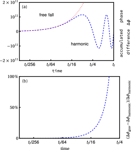
Figure 4: (a) Accumulated phase difference $\Delta\phi$ for one oscillation period $t_{f}=\frac{2\pi}{\omega}$. The blue dashed line corresponds to $\Delta\phi_{\text{harmonic}}$ in Eq. (66) which oscillates at frequency $2\omega$ completing two full oscillations in the trap oscillation period $t_{f}$. The red dotted line denotes the transient free fall phase $\Delta\phi_{\text{grav}}$ in Eq. (67). We have considered typical values considered in the main text: the nanoparticle mass $m=m_{n}\sim 10^{-15}\text{m}$, Paul trap frequency $\omega\sim 5\times 10^{-6}\text{Hz}$, initial position $x_{2}(0)=g_{e}/\omega^{2}\sim 4\times 10^{11}\text{m}$, initial momentum to $p_{2}(0)\sim 0,$ and superposition size $\Delta x=10^{-14}\text{m}$. We find that one period of oscillation is $t_{f}\sim 10^{6}\text{s}$. (b) Relative error between the full harmonic solution and the free fall approximation. The free-fall transient is a good approximation for $t\apprle t_{f}/10\sim 10^{5}\text{s}$, much longer than the time-scale of the experiment.

Using the notation of section (B) we consider the description from reference frame 2, i.e. the dynamics is purely harmonic with the Hamiltonian given in Eq. (12). Here for simplicity we consider the case $\omega=\omega_{1}=\omega_{2}$. The accumulated phase is given by the classical action

$$\phi[x_{2}(0),p_{2}(0)]=\frac{1}{\hbar}\int_{0}^{t}\left[\frac{p_{2}^{2}(s)}{2m}-\frac{m\omega^{2}}{2}x_{2}^{2}(s)\right]ds,$$ (63)

where $x_{2}$ and $p_{2}$ are given in Eqs. (13) and (14). Evaluating the integral we readily find:

$$\phi[x_{2}(0),p_{2}(0)]= \frac{\sin(2\omega t_{f})(p_{2}^{2}(0)-(m\omega(x_{2}(0))^{2})}{4m\omega\hbar}$$

$$-\frac{p_{2}(0)x_{2}(0)}{\hbar}\sin^{2}(\omega t).$$ (64)

We now consider the phase difference at different heights

$$\Delta\phi=-(\phi[x_{2}(0)+\Delta x,p_{2}(0)]-\phi[x_{2}(0),p_{2}(0)]),$$ (65)

Using Eq. (64) we immediately find

$$\Delta\phi_{\text{harmonic}}= \frac{\text{$\Delta x$}m\omega(\text{$\Delta x$}+2x_{2}(0))}{4\hbar}\sin(2\omega t)$$

$$+\frac{\text{$\Delta x$}p_{2}(0)}{\hbar}\sin^{2}(\omega t)$$ (66)

Let us expand the expression for small $\Delta x$ compared to $x_{2}(0)$ and to $\mathcal{O}(t)$, i.e. we are interested in the free-fall regime of tiny superpositions. We readily find

$$\Delta\phi_{\text{grav}}\approx \frac{\text{$\Delta x$}x_{2}(0)m\omega^{2}t}{\hbar}$$ (67)

Using $g_{e}=x_{2}(0)\omega^{2}$ we again recover Eq. (61) obtained from a more refined analysis. We have plotted in Fig. 4 a comparison between $\Delta\phi_{\text{harmonic}}$ and $\Delta\phi_{\text{grav}}$.

References

- [1] Erwin Schrödinger. Die gegenwartige Situation in der Quantenmechanik. Naturwiss., 23:807–812, 1935.
- [2] James Millen, Tania S Monteiro, Robert Pettit, and A Nick Vamivakas. Optomechanics with levitated particles. Reports on Progress in Physics, 83(2):026401, jan 2020.
- [3] Uroš Delić, Manuel Reisenbauer, Kahan Dare, David Grass, Vladan Vuletić, Nikolai Kiesel, and Markus Aspelmeyer. Cooling of a levitated nanoparticle to the motional quantum ground state. Science, 2020.
- [4] Felix Tebbenjohanns, Martin Frimmer, Vijay Jain, Dominik Windey, and Lukas Novotny. Motional sideband asymmetry of a nanoparticle optically levitated in free space. Physical Review Letters, 124(1):013603, 2020.
- [5] Angelo Bassi, Kinjalk Lochan, Seema Satin, Tejinder P Singh, and Hendrik Ulbricht. Models of wave-function collapse, underlying theories, and experimental tests. Reviews of Modern Physics, 85(2):471, 2013.
- [6] Sougato Bose, Anupam Mazumdar, Gavin W Morley, Hendrik Ulbricht, Marko Toroš, Mauro Paternostro, Andrew A Geraci, Peter F Barker, MS Kim, and Gerard Milburn. Spin entanglement witness for quantum gravity. Physical review letters, 119(24):240401, 2017.
- [7] Chiara Marletto and Vlatko Vedral. Gravitationally induced entanglement between two massive particles is sufficient evidence of quantum effects in gravity. Physical review letters, 119(24):240402, 2017.
- [8] Ryan J Marshman, Anupam Mazumdar, and Sougato Bose. Locality and entanglement in table-top testing of the quantum nature of linearized gravity. Physical Review A, 101(5):052110, 2020.
- [9] Bastian Hacker, Stephan Welte, Severin Daiss, Armin Shaukat, Stephan Ritter, Lin Li, and Gerhard Rempe. Deterministic creation of entangled atom–light schrödinger-cat states. Nature Photonics, 13(2):110–115, 2019.
- [10] Jason F Ralph, Marko Toroš, Simon Maskell, Kurt Jacobs, Muddassar Rashid, Ashley J Setter, and Hendrik Ulbricht. Dynamical model selection near the quantum-classical boundary. Physical Review A, 98(1):010102, 2018.
- [11] S Bose, K Jacobs, and PL Knight. Preparation of nonclassical states in cavities with a moving mirror. Physical Review A, 56(5):4175, 1997.
- [12] Sougato Bose, Kurt Jacobs, and Peter L Knight. Scheme to probe the decoherence of a macroscopic object. Physical Review A, 59(5):3204, 1999.
- [13] Oriol Romero-Isart, Anika C Pflanzer, Florian Blaser, Rainer Kaltenbaek, Nikolai Kiesel, Markus Aspelmeyer, and J Ignacio Cirac. Large quantum superpositions and interference of massive nanometer-sized objects. Physical review letters, 107(2):020405, 2011.
- [14] Michael R Vanner. Selective linear or quadratic optomechanical coupling via measurement. Physical Review X, 1(2):021011, 2011.
- [15] GA Brawley, MR Vanner, Peter Emil Larsen, Silvan Schmid, Anja Boisen, and WP Bowen. Nonlinear optomechanical measurement of mechanical motion. Nature communications, 7(1):1–7, 2016.
- [16] Jack Clarke and Michael R Vanner. Growing macroscopic superposition states via cavity quantum optomechanics. Quantum Science and Technology, 4(1):014003, 2018.
- [17] Shimon Kolkowitz, Ania C Bleszynski Jayich, Quirin P Unterreithmeier, Steven D Bennett, Peter Rabl, JGE Harris, and Mikhail D Lukin. Coherent sensing of a mechanical resonator with a single-spin qubit. Science, 335(6076):1603–1606, 2012.
- [18] Olivier Arcizet, Vincent Jacques, Alessandro Siria, Philippe Poncharal, Pascal Vincent, and Signe Seidelin. A single nitrogen-vacancy defect coupled to a nanomechanical oscillator. Nature Physics, 7(11):879–883, 2011.
- [19] Matteo Scala, MS Kim, GW Morley, PF Barker, and S Bose. Matter-wave interferometry of a levitated thermal nano-oscillator induced and probed by a spin. Physical review letters, 111(18):180403, 2013.
- [20] Zhang-qi Yin, Tongcang Li, Xiang Zhang, and LM Duan. Large quantum superpositions of a levitated nanodiamond through spin-optomechanical coupling. Physical Review A, 88(3):033614, 2013.
- [21] C Wan, M Scala, GW Morley, ATM A Rahman, H Ulbricht, J Bateman, PF Barker, S Bose, and MS Kim. Free nano-object ramsey interferometry for large quantum superpositions. Physical review letters, 117(14):143003, 2016.
- [22] Christopher Monroe, DM Meekhof, BE King, and David J Wineland. A "Schrödinger cat" superposition state of an atom. Science, 272(5265):1131–1136, 1996.
- [23] Klemens Hammerer, Kai Stannigel, Claudiu Genes, Peter Zoller, Philipp Treutlein, Stephan Camerer, David Hunger, and Theodor W Hänsch. Optical lattices with micromechanical mirrors. Physical Review A, 82(2):021803, 2010.
- [24] Berit Vogell, Kai Stannigel, Peter Zoller, Klemens Hammerer, Matthew T Rakher, Maria Korppi, Andreas Jöckel, and Philipp Treutlein. Cavity-enhanced long-distance coupling of an atomic ensemble to a micromechanical membrane. Physical Review A, 87(2):023816, 2013.
- [25] James S Bennett, Lars S Madsen, Mark Baker, Halina Rubinsztein-Dunlop, and Warwick P Bowen. Coherent control and feedback cooling in a remotely coupled hybrid atom–optomechanical system. New Journal of Physics, 16(8):083036, 2014.
- [26] Gambhir Ranjit, Cris Montoya, and Andrew A Geraci. Cold atoms as a coolant for levitated optomechanical systems. Physical Review A, 91(1):013416, 2015.
- [27] Markus Rademacher, James Millen, and Ying Lia Li. Quantum sensing with nanoparticles for gravimetry: when bigger is better. Advanced Optical Technologies, 9(5):227–239, 2020.
- [28] Rudolf Grimm, Matthias Weidemüller, and Yurii B Ovchinnikov. Optical dipole traps for neutral atoms. In Advances in atomic, molecular, and optical physics, volume 42, pages 95–170. Elsevier, 2000.
- [29] Kane Yee. Numerical solution of initial boundary value problems involving maxwell’s equations in isotropic media. IEEE Transactions on Antennas and Propagation, 14(3):302–307, 1966.
- [30] Lumerical inc. fdtd 3d electromagnetic simulator. https://www.lumerical.com/products/, 2019.
- [31] David J Wineland, C Monroe, Wayne M Itano, Dietrich Leibfried, Brian E King, and Dawn M Meekhof. Experimental issues in coherent quantum-state manipulation of trapped atomic ions. Journal of Research of the National Institute of Standards and Technology, 103(3):259, 1998.
- [32] Wayne M Itano, Christopher R Monroe, DM Meekhof, D Leibfried, BE King, and David J Wineland. Quantum harmonic oscillator state synthesis and analysis. In Atom Optics, volume 2995, pages 43–55. International Society for Optics and Photonics, 1997.
- [33] Erik Hebestreit, Martin Frimmer, René Reimann, and Lukas Novotny. Sensing static forces with free-falling nanoparticles. Physical review letters, 121(6):063602, 2018.
- [34] NP Bullier, A Pontin, and PF Barker. Characterisation of a charged particle levitated nano-oscillator. Journal of Physics D: Applied Physics, 53(17):175302, 2020.
- [35] A. Pontin, N. P. Bullier, M. Toroš, and P. F. Barker. An ultra-narrow line width levitated nano-oscillator for testing dissipative wavefunction collapse, 2019.
- [36] Oriol Romero-Isart. Coherent inflation for large quantum superpositions of levitated microspheres. New Journal of Physics, 19(12):123029, 2017.
- [37] Erik Hebestreit, René Reimann, Martin Frimmer, and Lukas Novotny. Measuring the internal temperature of a levitated nanoparticle in high vacuum. Physical Review A, 97(4):043803, 2018.
- [38] ATM Anishur Rahman and PF Barker. Laser refrigeration, alignment and rotation of levitated yb 3+: Ylf nanocrystals. Nature Photonics, 11(10):634–638, 2017.
- [39] Maximilian A Schlosshauer. Decoherence: and the quantum-to-classical transition. Springer Science & Business Media, 2007.
- [40] Oriol Romero-Isart. Quantum superposition of massive objects and collapse models. Physical Review A, 84(5):052121, 2011.
- [41] T Seberson and F Robicheaux. Distribution of laser shot noise energy delivered to a levitated nanoparticle. arXiv preprint arXiv:1909.06469, 2019.
- [42] Paul S Epstein. On the resistance experienced by spheres in their motion through gases. Physical Review, 23(6):710, 1924.
- [43] A Cavalleri, G Ciani, R Dolesi, M Hueller, D Nicolodi, D Tombolato, S Vitale, PJ Wass, and WJ Weber. Gas damping force noise on a macroscopic test body in an infinite gas reservoir. Physics Letters A, 374(34):3365–3369, 2010.
- [44] Yaakov Y Fein, Philipp Geyer, Patrick Zwick, Filip Kiałka, Sebastian Pedalino, Marcel Mayor, Stefan Gerlich, and Markus Arndt. Quantum superposition of molecules beyond 25 kda. Nature Physics, 15(12):1242–1245, 2019.
- [45] Rudolf Grimm, Matthias Weidemüller, and Yurii B. Ovchinnikov. Optical dipole traps for neutral atoms. volume 42 of Advances In Atomic, Molecular, and Optical Physics, pages 95 – 170. Academic Press, 2000.
- [46] VI Balykin, VG Minogin, and VS Letokhov. Electromagnetic trapping of cold atoms. Reports on Progress in Physics, 63(9):1429, 2000.
- [47] Dietrich Leibfried, Rainer Blatt, Christopher Monroe, and David Wineland. Quantum dynamics of single trapped ions. Reviews of Modern Physics, 75(1):281, 2003.
- [48] Soo Chang and V Minogin. Density-matrix approach to dynamics of multilevel atoms in laser fields. Physics Reports, 365(2):65–143, 2002.
- [49] BM Garraway and VG Minogin. Theory of an optical dipole trap for cold atoms. Physical Review A, 62(4):043406, 2000.
- [50] Jin Woo Jun and VG Minogin. Stability of the far-off-resonance dipole-atom trap with superimposed laser cooling. Physical Review A, 64(2):023413, 2001.
- [51] Xin Ma and William Rhodes. Squeezing in harmonic oscillators with time-dependent frequencies. Physical Review A, 39(4):1941, 1989.
- [52] Pippa Storey and Claude Cohen-Tannoudji. The feynman path integral approach to atomic interferometry. a tutorial. Journal de Physique II, 4(11):1999–2027, 1994.