Supermassive Binary Black Hole Evolution
can be traced by a small SKA Pulsar Timing Array

Abstract

Supermassive black holes are commonly found in the center of galaxies and evolve with their hosts. The supermassive binary black holes (SMBBH) are thus expected to exist in close galaxy pairs, however, none has been unequivocally detected. The square kilometre array (SKA) is a multi-purpose radio telescope with a collecting area approaching 1 million square metres, with great potential for detecting nanohertz gravitational waves (GWs). In this paper, we quantify the GW detectability by SKA for a realistic SMBBH population using pulsar timing array (PTA) technique and quantify its impact on revealing SMBBH evolution with redshift for the first time. With only $\sim 20$ pulsars, much smaller a requirement than in previous work, the SKA PTA is expected to obtain detection within about 5 years of operation and to achieve a detection rate of more than 100 SMBBHs/yr after about 10 years. Although beyond the scope of this paper, we must acknowledge that the presence of persistent red noise will reduce the number of expected detections here. It is thus imperative to understand and mitigate red noise in the PTA data. The GW signatures from a few well-known SMBBH candidates, such as OJ 287, 3C 66B, NGC 5548 and Ark 120, will be detected given the currently best-known parameters of each system. Within 30 years of operation, about 60 individual SMBBHs detection with $z<0.05$ and more than $10^{4}$ with $z<1$ are expected. The detection rate drops precipitately beyond $z=1$. The substantial number of expected detections and their discernible evolution with redshift by SKA PTA will make SKA a significant tool for studying SMBBHs.

abcd

1 Introduction

GW observatories such as advanced LIGO (aLIGO) (LIGO Scientific Collaboration et al., 2015) and Virgo (Acernese et al., 2015) have reached remarkable sensitivities in the high frequency band ($\sim 10-1000\,\rm Hz$). The detection of GWs from compact binary mergers has become a regular occurrence. In the nanohertz frequency band, pulsar timing arrays (PTAs), in which a collection of millisecond pulsars is monitored, can be used to detect and study GWs Detweiler (1979); Foster & Backer (1990). The primary single source of GWs in nanohertz band are believed to be inspiralling SMBBHs, formed in the aftermath of galaxy mergers (Begelman et al., 1980). The detection of SMBBH systems can yield direct information about the masses and spins of the black holes (Mingarelli et al., 2012). These single GW sources can also be studied by coordinated electromagnetic observations, thus enabling a multi-messenger view of the black hole systems Burke-Spolaor (2013); Kelley et al. (2019).

PTA based GW astronomy is expected to progress significantly with the new and high sensitivity radio telescopes such as FAST (Nan et al., 2011) and SKA (Smits et al., 2009). The pulsar timing effort by SKA will significantly enhance the sensitivity of the current PTA networks by providing a larger number of newly discovered millisecond pulsars (MSPs), and better timing precision on the existing and new MSPs. Upon its completion, SKA will be the most sensitive telescope for detecting nanohertz GWs in the next generation. Thus, it is important to estimate the GW detection abilities of SKA. Wang & Mohanty (Wang & Mohanty, 2017) carried out a pioneering quantitative assessment of the GW detectability for individual SMBBH searches with a simulated SKAPTA containing $10^{3}$ pulsars and found the SKAPTA to significantly increase the maximum distance of detectable GWs emitted by SMBBHs. They also considered two realistic candidates, namely, PG 1302-102 and PSO J334+01. However, no previous work has provide actual predictions of the number of SMBBHs to be detected by SKAPTA and their evolution through redshifts.

Here we provide one of the first quantitative estimates on the GW detectability for a realistic individual SMBBH population. We tackle the problem in three steps. First, a SKAPTA detection curve, namely the minimum detectable GW strain amplitude as a function of GW frequency, is calculated. A SKAPTA containing 20 randomly placed pulsars with timing root mean square (RMS) of 20 ns is used to compute the detection curves, using the $\mathcal{F}_{e}$ statistic, the logarithm of the likelihood ratio maximized over the signal parameters developed by Jaranowski et al. (1998); Ellis et al. (2012). Here we assume circular binary orbits for the SMBBHs. Second, an expected SMBBH population in the PTA frequency band is constructed based on the probability of a galaxy hosting a SMBBH in the PTA band and the population of host galaxies. The SMBBH population is estimated following the descriptions of Mingarelli et al. (2017); Mingarelli (2017) (hereafter M17). M17 used data from local galaxies in the 2 Micron All Sky Survey (2MASS) (Skrutskie et al., 2006) Extended Source Catalog (Jarrett et al., 2000) and galaxy merger rates from Illustris Rodriguez-Gomez et al. (2015); Genel et al. (2014). Due to the expected great improvement brought about by SKAPTA, we much extend the redshift range in M17 using galaxy stellar mass function from Bell et al. (2003); Muzzin et al. (2013) (GSMF). Third, we extract detectable GW sources within each redshift bin according to the SKAPTA detection curve calculated above and the expected SMBBH population estimated in step two. Our recipe allows for a quantitative prediction of the properties of the SMBBH population to be detected by SKAPTA, such as the number of detections per redshift bin and detection rates per year, for the first time.

2 Simulated SKAPTA

With broad frequency bands and massive collecting areas, the radiometer noise for some of the brightest pulsars can be reduced from current 100 ns level down to below 10 ns by the large radio telescopes like FAST and SKA. Jitter noise, which is assumed to be caused by the fluctuation in the shape and arrival time of individual pulses, will limit the timing precision achievable over data spans of a few years for these large facilities (Hobbs et al., 2019). To estimate the timing RMS, we assume that the timing RMS is white and consists solely of radiometer noise and jitter noise. We defer the influence of red noise (e.g. GWB, dispersion measure variation noise, intrinsic timing noise (Hobbs et al., 2019)) to later discussions. Table 4 in (Porayko et al., 2018) listed white noise for 10 Parkes Pulsar Timing Array (PPTA) (Manchester et al., 2013) pulsars with a harmonic mean of 20 ns for integration time of 30 minutes with the SKA Phase 1(Janssen et al., 2015). Within the SKA sky, International Pulsar Timing Array (IPTA)(Manchester & IPTA, 2013) source list contains more millisecond pulsars than PPTA does. For example, IPTA PSR J0023+0923, PSR J0030+0451, PSR J0931$-$1902 are not in the PPTA line-up. Considering the better sensitivity of the full SKA than that of SKA Phase 1, which will further improve timing RMS, we assume a conservative 20 pulsars with a harmonic mean of 20 ns. We thus construct a mock SKAPTA data set containing 20 millisecond pulsars randomly distributed in the sky. Noise realizations are drawn from an independent and identically distributed (i.i.d.) $\mathcal{N}(0,\sigma^{2})$ (zero mean white Gaussian noise) process, with $\sigma=20$ ns for all pulsars. We choose the cadence to be 20 $\rm{yr}^{-1}$ in order to match the typical cadence used in current PTAs.

3 SMBBH population in the PTA band

The SMBBH population emitting in the PTA frequency band depends on two quantities:

1. The probability of a galaxy hosting a SMBBH in the PTA band. We exploit the approach put forward by M17 (See M17 for details of the approach). The probability is the multiplication of the probability that a SMBBH is in the PTA band and the probability that a galaxy hosts a SMBBH. The probability that a SMBBH is in the PTA band is $t_{\mathrm{obs}}/T_{\mathrm{life}}$, where $t_{\mathrm{obs}}=5/256c^{5}(\pi f)^{-8/3}{[GM_{c}(1+z)]}^{-5/3}$ is the time to coalescence of the binary in the observed frame (Peters, 1964). Here $f=1\,\mathrm{nHz}$, chirp mass $M_{c}=\left[q/(1+q)^{2}\right]^{3/5}M_{\bullet}$ with black hole mass ratio $q$ drawn from a log-uniform distribution in $[0.25,1]$. The SMBBH total mass $M_{\bullet}$ is estimated using the $M_{\bullet}-M_{\mathrm{bulge}}$ empirical scaling relation from (McConnell & Ma, 2013). As discussed in M17, only massive early-type galaxies are considered in this simulation, therefore we take the galaxy stellar mass $M_{*}$ as $M_{\mathrm{bulge}}$ for $M_{\bullet}$ estimates. $T_{\mathrm{life}}$ is the effective lifetime of the binary, which is the sum of the dynamical friction ($t_{\mathrm{df}}$) (Binney & Tremaine, 2008) and stellar hardening ($t_{\mathrm{sh}}$) (Sesana & Khan, 2015) timescales. The probability that a galaxy hosts SMBBH is computed using the Illustris Rodriguez-Gomez et al. (2015); Genel et al. (2014) cumulative galaxy-galaxy merger rate, $\mathrm{d}N/\mathrm{d}t(M_{*},z^{\prime},\mu_{*})$ where $\mu_{*}$ is the stellar mass ratio of the galaxies, taken at the beginning of the binary evolution at redshift $z^{\prime}$, which is calculated at lookback time of $T_{\mathrm{life}}+T_{\mathrm{lookback}}$ with Planck cosmological parameters (Planck Collaboration et al., 2016), here $T_{\mathrm{lookback}}$ is the lookback time at $z$. To summarize, probability of a galaxy hosting a SMBBH in the PTA band is:

   $$p=\frac{t_{\mathrm{obs}}}{T_{\mathrm{life}}}\int_{0.25}^{1}\mathrm{d}\mu_{*}\frac{\mathrm{d}N}{\mathrm{d}t}(M_{*},z^{\prime},\mu_{*})T_{\mathrm{life}}\,,$$ (1)

2. The population of host galaxies. As discussed in M17, we only consider massive early-type galaxies with galaxy stellar mass greater than $10^{11}\,\rm M_{\odot}$. In addition, we impose a cut on the galaxy population at galaxy stellar mass $M_{*}<10^{12}\,\rm M_{\odot}$ because such massive galaxies are rare. For a population of galaxy with known redshift $z$ and $M_{*}$, we can calculate the probability of a selected galaxy hosting a SMBBH in the PTA band using Eq. 1, and thus determining the population of SMBBH emitting in the PTA frequency band. For galaxies at $z<0.05$, we use the galaxy catalog in M17, which selected galaxies at $z<0.05$ from the 2 Micron All Sky Survey (2MASS) (Skrutskie et al., 2006) Extended Source Catalog (Jarrett et al., 2000). To approximate a mass selection for more distant galaxies, we use GSMF given in Table 4 of (Bell et al., 2003) and Table 1 of (Muzzin et al., 2013) for redshift interval between $z$ = 0.05, 0.2, 0.5, 1.0, 1.5, 2.0, 2.5, 3.0, and 4.0. For each $z$ interval at $z>0.05$, we randomly choose $10^{6}$ host galaxies with $z$ drawn from a uniform distribution and stellar mass drawn from the corresponding GSMF. The number of $10^{6}$ galaxies is used to ensure stable simulation results in the Monte Carlo process. The estimated numbers of galaxies in each redshift bin is then scaled to the expected galaxy population from the sample of $10^{6}$ galaxies in the simulation. Using Eq. 1, we calculate the probability of a selected galaxy hosting a SMBBH in the PTA band. We then generate a random number from $U$[0, 1], if the random number is smaller than the probability, then the galaxy is considered to host a true SMBBH. Finally, the inclination and polarization-averaged strain and GW frequency of the SMBBH are calculated as described in M17 using

   $$h=\sqrt{\frac{32}{5}}\frac{{M}_{c}^{5/3}}{D_{c}}\left[\pi f(1+z)\right]^{2/3}\,,$$ (2)

   $$f=\pi^{-1}\left[\frac{G{M}_{c}(1+z)}{c^{3}}\right]^{-5/8}\left[\frac{256}{5}(t_{\mathrm{obs}}-t)\right]^{-3/8}\,,$$ (3)

   where $D_{c}$ is the comoving distance of the binary, $(t_{\mathrm{obs}}-t)$ is drawn from a uniform distribution in $[26~{}\rm{Myr},100~{}\rm{yr}]$.

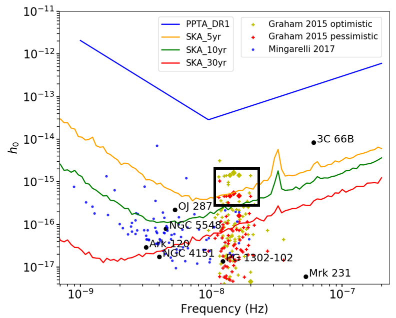
Figure 1: Detection curves for PPTA_DR1 (blue line), SKA_5yr (orange line), SKA_10yr (green line), SKA_30yr (red line) respectively. The seven black dots represent the SMBBH candidates discussed in (Feng et al., 2019). The yellow (best case) and red (pessimistic case) dots (’+’ for $z<2$ samples and diamond symbol for $z>2$) represent CRTS samples. The diamond symbols in the black box represent 4 unreliable candidates (two overlapped, see the text for details). The blue dots represent 87 single GW sources (one realization of sky) from M17.

4 Results

We use the $\mathcal{F}_{e}$ statistic with False Alarm Probability of $10^{-3}$ to calculate detection curves for SKAPTA with total time span of 5, 10, 30 yrs respectively. The results are shown in Figure 1. The SMBBH candidates such as 3C 66B (Iguchi et al., 2010), OJ 287 (Valtonen et al., 2016), NGC 5548 (Li et al., 2016) and Ark 120 (Li et al., 2019) (black dots in Figure 1) discussed in (Feng et al., 2019) can be detected if they are true SMBBHs. For the other SMBBH candidates Mrk 231 (Yan et al., 2015), PG 1302-102 (Graham et al., 2015a), NGC 4151 (Bon et al., 2012), they are hard to detect even in SKA era for their weaker estimated GW signature caused by their small chirp masses. (Graham et al., 2015b) proposed 111 SMBBH candidates by inspecting the light curves of $\sim$250 k quasars identified in the Catalina Real-time Transient Survey (CRTS, Drake et al. (2009)). We plot the 98 candidates (hereafter CRTS samples) with reported black hole mass estimates for optimistic case assuming mass ratio $q=1$ (yellow dots in Figure 1) and pessimistic case assuming $q=0.1$ (red dots in Figure 1). At least 10 single sources in CRTS samples can be detected, assuming these are all true sources, even for the pessimistic case. Unfortunately, CRTS samples are likely contaminated by several false positives Sesana et al. (2018) and we will discuss this later. The blue dots represent 87 single GW sources (one realization of sky) from M17. 0, 2, 12, 64 sources of M17 can be detected for PPTA_DR1, SKA_5yr, SKA_10yr, SKA_30yr.

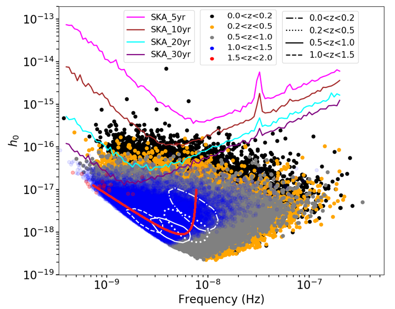
Figure 2: Detection curves for SKA_5yr (magenta line), SKA_10yr (brown line), SKA_20yr (cyan line), SKA_30yr (purple line) respectively. Black, orange, gray, blue, red dots represent SMBBH population hosted by $10^{6}$ galaxies from $0.0<z<0.2$, $0.2<z<0.5$, $0.5<z<1.0$, $1.0<z<1.5$, $1.5<z<2.0$ respectively (for $0.0<z<0.2$, it is 87 SMBBHs from M17 combined with SMBBH population hosted by $10^{6}$ galaxies from $0.05<z<0.2$). Dashdot, dotted, solid, dashed number density contours represent 50% of the peak value for $0.0<z<0.2$, $0.2<z<0.5$, $0.5<z<1.0$, $1.0<z<1.5$ respectively. For $z>2.0$, there are no detectable SMBBHs in the PTA band, so SMBBH population at $z>2.0$ is not shown in the figure. The red curve cross the contour centers shows the evolution trend of SMBBH population from low redshift to high redshift.

Figure 2 shows the SMBBH population in the PTA band. In Figure 2, we also plot the 5, 10, 20, 30 yr detection curves to show the potential detectability of these single GW sources. The strain of the population shifts to a low value at $z\lesssim 0.5$ for higher redshift due to their further distance. The frequency of the population shifts to lower frequency at $z\gtrsim 0.5$ because these SMBBHs do not have enough time to evolve to be closer, with higher redshift SMBBHs have less time to evolve. Given the detection curves and SMBBH population in the PTA band, we determine the detection number of single GW sources as a function of SKAPTA time span. The source is considered detected if it lies above the detection curve. The total number of host galaxies is the multiplication of comoving volume and integral of the corresponding GSMF from $10^{11}\,\rm M_{\odot}$ to $10^{12}\,\rm M_{\odot}$, and is listed in the last row of Table 1. The number of SMBBHs in the PTA band is listed in the second last row.

Figure 3 shows detection number for different redshift ranges as a function of SKAPTA time span. We list the detection number for different redshift ranges of 5, 10, 15, 20, 30 time span SKAPTA in Table 1. More than $10^{4}$ sources can be detected by SKAPTA after 30 years of operation. The primary detectable sources come from galaxies at $z<1$. Detectable sources at $z>1.5$ are rare as their larger distances dampen the apparent GW signal. Some of them also did not have enough time to evolve to be close enough, thus have a longer observed orbital period outside of the PTA frequency band. The dramatic drops of GW detection at $z>1.5$ is consistent with Sesana (2013); Ravi et al. (2015). Moreover, no hosts at $z>2.0$ are expected to have detectable SMBBHs in our simulation. If this result is true, it implies that CRTS samples at $z>2.0$ may not be real SMBBHs. For example, Table 1 in Sesana et al. (2018) listed top 10 candidates in CRTS samples providing the largest contribution to the expected GWB, which are likely to be false positives. In this sample, four of them (i.e., HS 0926+3608, SDSS J140704.43+273556.6, SDSS J131706.19+271416.7, SDSS J134855.27-032141.4) have redshifts $z>2.0$ and are shown using diamond symbols inside the black box in Figure 1. Combining our results and Sesana et al. (2018), these 4 candidates can be unreliable.

Table 1: detection number

	$0.0<z<0.05$	$0.05<z<0.2$	$0.2<z<0.5$	$0.5<z<1.0$	$1.0<z<1.5$	$1.5<z<2.0$
5	2	0	0	0	0	0
10	12	81	26	0	0	0
15	35	593	221	102	25	13
20	57	3017	2067	884	250	13
30	64	6726	17329	11356	3925	39
total SMBBHs	87	$1.0\times 10^{5}$	$1.0\times 10^{6}$	$3.4\times 10^{6}$	$8.4\times 10^{5}$	$2.6\times 10^{2}$
total hosts	5119	$1.6\times 10^{6}$	$1.3\times 10^{7}$	$3.4\times 10^{7}$	$2.5\times 10^{7}$	$1.3\times 10^{7}$

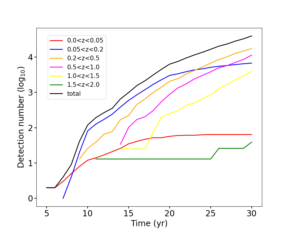
Figure 3: Detection number of single GW sources versus time span of SKAPTA. The red, blue, orange, magenta, yellow, green, black colors represent number of sources at $0.0<z<0.05$, $0.05<z<0.2$, $0.2<z<0.5$, $0.5<z<1.0$, $1.0<z<1.5$, $1.5<z<2.0$ and total number respectively.

We calculate the detection rate as a function of SKAPTA time span by comparing the detection number of two consecutive years. The results are shown in Figure 4. Unlike GW sources in LIGO frequency band, the detection rate of single GW sources of SKAPTA is not uniform in time. The detectability increases slowly in the early times, but increases faster to be more than 100 detections/yr after about 10 yrs. This is a stipend from the unique PTA based search, which accumulates SNR with time, highlighting the importance of long time span of a PTA campaign.

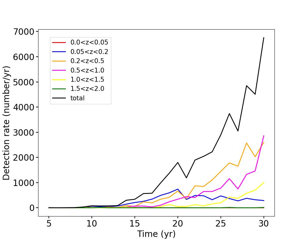
Figure 4: Detection rate of single GW sources versus time span of SKAPTA. The red, blue, orange, magenta, yellow, green, black colors represent number of sources at $0.0<z<0.05$, $0.05<z<0.2$, $0.2<z<0.5$, $0.5<z<1.0$, $1.0<z<1.5$, $1.5<z<2.0$ and total rate respectively.

5 Discussion

Red noise was ignored under the assumption that it can be mitigated to a low noise level or it does not influence single GW detection using special techniques. If the timing residuals have a strong red noise component emulating an unresolved GWB with amplitude of $4\times 10^{-16}$, the detection number decreases drastically as shown in Figure 5. This is because PTA is less sensitive to high frequency ($>1\,\rm{yr}^{-1}$) SMBBHs, and strong red noise in timing residuals greatly diminishes the chance of detecting lower frequency SMBBHs. The SKAPTA GW detections depend on how well the GWB can be subtracted, which should be further studied. The methodology of GWB subtraction is also important to mitigate other various types of red noises which could limit the detectability of SMBBHs with SKAPTA.

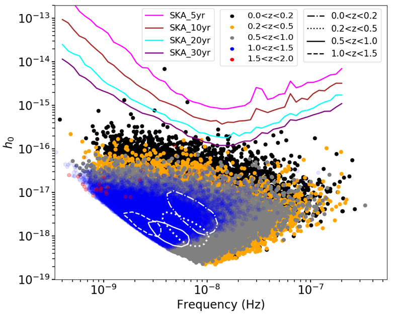
Figure 5: Same as Fig. 2, but timing residuals have a strong red noise component of $4\times 10^{-16}$, emulating the amplitude of an unresolved GWB.

6 Conclusion

The unprecedented sensitivity of SKA facilitates realization of a significant PTA with a small number of pulsars. The SKAPTA in this work consists of only 20 pulsars versus $\sim 1000$ in previous works. Such a simple SKAPTA can still detect a large number of SMBBHs and enable studies of their evolution through redshift up to $z=1-2$ assuming red noise in the PTA data can be mitigated. The presence of red noise will reduce the number of detectable individual sources. Nevertheless, SKAPTA will be a revolutionary instrument for studying SMBBH evolution.

References

- Acernese et al. (2015) Acernese, F., Agathos, M., Agatsuma, K., et al. 2015, Classical and Quantum Gravity, 32, 024001, doi: 10.1088/0264-9381/32/2/024001
- Begelman et al. (1980) Begelman, M. C., Blandford, R. D., & Rees, M. J. 1980, Nature, 287, 307, doi: 10.1038/287307a0
- Bell et al. (2003) Bell, E. F., McIntosh, D. H., Katz, N., & Weinberg, M. D. 2003, ApJ Supplements, 149, 289, doi: 10.1086/378847
- Binney & Tremaine (2008) Binney, J., & Tremaine, S. 2008, Galactic Dynamics: Second Edition (Princeton University Press)
- Bon et al. (2012) Bon, E., Jovanović, P., Marziani, P., et al. 2012, ApJ, 759, 118, doi: 10.1088/0004-637X/759/2/118
- Burke-Spolaor (2013) Burke-Spolaor, S. 2013, Classical and Quantum Gravity, 30, 224013, doi: 10.1088/0264-9381/30/22/224013
- Detweiler (1979) Detweiler, S. 1979, ApJ, 234, 1100, doi: 10.1086/157593
- Drake et al. (2009) Drake, A. J., Djorgovski, S. G., Mahabal, A., et al. 2009, ApJ, 696, 870, doi: 10.1088/0004-637X/696/1/870
- Ellis et al. (2012) Ellis, J. A., Siemens, X., & Creighton, J. D. E. 2012, ApJ, 756, 175, doi: 10.1088/0004-637X/756/2/175
- Feng et al. (2019) Feng, Y., Li, D., Li, Y.-R., & Wang, J.-M. 2019, arXiv e-prints, arXiv:1907.03460. https://arxiv.org/abs/1907.03460
- Foster & Backer (1990) Foster, R. S., & Backer, D. C. 1990, ApJ, 361, 300, doi: 10.1086/169195
- Genel et al. (2014) Genel, S., Vogelsberger, M., Springel, V., et al. 2014, MNRAS, 445, 175, doi: 10.1093/mnras/stu1654
- Graham et al. (2015a) Graham, M. J., Djorgovski, S. G., Stern, D., et al. 2015a, Nature, 518, 74, doi: 10.1038/nature14143
- Graham et al. (2015b) —. 2015b, MNRAS, 453, 1562, doi: 10.1093/mnras/stv1726
- Hobbs et al. (2019) Hobbs, G., Dai, S., Manchester, R. N., et al. 2019, Research in Astronomy and Astrophysics, 19, 020, doi: 10.1088/1674-4527/19/2/20
- Iguchi et al. (2010) Iguchi, S., Okuda, T., & Sudou, H. 2010, ApJ Letters, 724, L166, doi: 10.1088/2041-8205/724/2/L166
- Janssen et al. (2015) Janssen, G., Hobbs, G., McLaughlin, M., et al. 2015, in Advancing Astrophysics with the Square Kilometre Array (AASKA14), 37. https://arxiv.org/abs/1501.00127
- Jaranowski et al. (1998) Jaranowski, P., Królak, A., & Schutz, B. F. 1998, Phys. Rev. D, 58, 063001, doi: 10.1103/PhysRevD.58.063001
- Jarrett et al. (2000) Jarrett, T. H., Chester, T., Cutri, R., et al. 2000, AJ, 119, 2498, doi: 10.1086/301330
- Kelley et al. (2019) Kelley, L., Charisi, M., Burke-Spolaor, S., et al. 2019, in BAAS, Vol. 51, 490. https://arxiv.org/abs/1903.07644
- Li et al. (2016) Li, Y.-R., Wang, J.-M., Ho, L. C., et al. 2016, ApJ, 822, 4, doi: 10.3847/0004-637X/822/1/4
- Li et al. (2019) Li, Y.-R., Wang, J.-M., Zhang, Z.-X., et al. 2019, ApJ Supplements, 241, 33, doi: 10.3847/1538-4365/ab0ec5
- LIGO Scientific Collaboration et al. (2015) LIGO Scientific Collaboration, Aasi, J., Abbott, B. P., et al. 2015, Classical and Quantum Gravity, 32, 074001, doi: 10.1088/0264-9381/32/7/074001
- Manchester & IPTA (2013) Manchester, R. N., & IPTA. 2013, Classical and Quantum Gravity, 30, 224010, doi: 10.1088/0264-9381/30/22/224010
- Manchester et al. (2013) Manchester, R. N., Hobbs, G., Bailes, M., et al. 2013, ApJ, 30, e017, doi: 10.1017/pasa.2012.017
- McConnell & Ma (2013) McConnell, N. J., & Ma, C.-P. 2013, ApJ, 764, 184, doi: 10.1088/0004-637X/764/2/184
- Mingarelli (2017) Mingarelli, C. 2017, ChiaraMingarelli/nanohertz_GWs: First release!, doi: 10.5281/zenodo.838712
- Mingarelli et al. (2012) Mingarelli, C. M. F., Grover, K., Sidery, T., Smith, R. J. E., & Vecchio, A. 2012, Physical Review Letters, 109, 081104, doi: 10.1103/PhysRevLett.109.081104
- Mingarelli et al. (2017) Mingarelli, C. M. F., Lazio, T. J. W., Sesana, A., et al. 2017, Nature Astronomy, 1, 886, doi: 10.1038/s41550-017-0299-6
- Muzzin et al. (2013) Muzzin, A., Marchesini, D., Stefanon, M., et al. 2013, ApJ, 777, 18, doi: 10.1088/0004-637X/777/1/18
- Nan et al. (2011) Nan, R., Li, D., Jin, C., et al. 2011, International Journal of Modern Physics D, 20, 989, doi: 10.1142/S0218271811019335
- Peters (1964) Peters, P. C. 1964, Physical Review, 136, 1224, doi: 10.1103/PhysRev.136.B1224
- Planck Collaboration et al. (2016) Planck Collaboration, Ade, P. A. R., Aghanim, N., et al. 2016, A&A, 594, A13, doi: 10.1051/0004-6361/201525830
- Porayko et al. (2018) Porayko, N. K., Zhu, X., Levin, Y., et al. 2018, Phys. Rev. D, 98, 102002, doi: 10.1103/PhysRevD.98.102002
- Ravi et al. (2015) Ravi, V., Wyithe, J. S. B., Shannon, R. M., & Hobbs, G. 2015, MNRAS, 447, 2772, doi: 10.1093/mnras/stu2659
- Rodriguez-Gomez et al. (2015) Rodriguez-Gomez, V., Genel, S., Vogelsberger, M., et al. 2015, MNRAS, 449, 49, doi: 10.1093/mnras/stv264
- Sesana (2013) Sesana, A. 2013, MNRAS, 433, L1, doi: 10.1093/mnrasl/slt034
- Sesana et al. (2018) Sesana, A., Haiman, Z., Kocsis, B., & Kelley, L. Z. 2018, ApJ, 856, 42, doi: 10.3847/1538-4357/aaad0f
- Sesana & Khan (2015) Sesana, A., & Khan, F. M. 2015, MNRAS, 454, L66, doi: 10.1093/mnrasl/slv131
- Skrutskie et al. (2006) Skrutskie, M. F., Cutri, R. M., Stiening, R., et al. 2006, AJ, 131, 1163, doi: 10.1086/498708
- Smits et al. (2009) Smits, R., Kramer, M., Stappers, B., et al. 2009, A&A, 493, 1161, doi: 10.1051/0004-6361:200810383
- Valtonen et al. (2016) Valtonen, M. J., Zola, S., Ciprini, S., et al. 2016, ApJ Letters, 819, L37, doi: 10.3847/2041-8205/819/2/L37
- Wang & Mohanty (2017) Wang, Y., & Mohanty, S. D. 2017, Physical Review Letters, 118, 151104, doi: 10.1103/PhysRevLett.118.151104
- Yan et al. (2015) Yan, C.-S., Lu, Y., Dai, X., & Yu, Q. 2015, ApJ, 809, 117, doi: 10.1088/0004-637X/809/2/117