Kondo breakdown in a spin-1/2 chain of adatoms on a Dirac semimetal

Abstract

We consider a spin-1/2 Heisenberg chain coupled via a Kondo interaction to two-dimensional Dirac fermions. The Kondo interaction is irrelevant at the decoupled fixed-point, leading to the existence of a Kondo-breakdown phase and a Kondo-breakdown critical point separating such a phase from a heavy Fermi liquid. We reach this conclusion on the basis of a renormalization group analysis, large-N calculations as well as extensive auxiliary-field quantum Monte Carlo simulations. We extract quantities such as the zero-bias tunneling conductance which will be relevant to future experiments involving adatoms on semimetals such as graphene.

The antiferromagnetic Kondo coupling, $J_{k}$, between a spin-1/2 degree of freedom and a Fermi sea with finite density of states at the Fermi energy is (marginally) relevant: $J_{k}$ flows to strong coupling and the impurity is screened. If, in contrast, the density of states shows a power-law pseudogap behavior, the Kondo coupling is irrelevant at the decoupled fixed point, and the spin remains unscreened at weak coupling. Since for large Kondo coupling screening is present, a novel Kondo-breakdown quantum critical point emerges [Withoff and Fradkin, 1990, Fritz and Vojta, 2004, Fritz and Vojta, 2013]. The decoupled as well as Kondo-screened phase share the same symmetry properties.

In the context of Kondo lattices, the numbers of both conduction electrons and impurity spins scale with the volume of the system. In the Kondo-screened paramagnetic (i.e. heavy Fermi liquid) phase, the volume enclosed by the Fermi surface (i.e. Luttinger volume) counts both spins and electrons. A Kondo-breakdown transition (equivalently, an orbital-selective Mott transition [Vojta, 2010]), which, as above, does not involve symmetry breaking, implies that the spins drop out from the Luttinger count. For the case of an odd number of electrons and spins per unit cell, this leads to a violation of the Luttinger sum rule. Oshikawa’s flux-threading argument [Yamanaka et al., 1997, Oshikawa, 2000] shows that a specific family of the resulting states of matter can be achieved via topological degeneracy in the spin sector [Senthil et al., 2003]. Such states, coined fractionalized Fermi liquid (FL^∗) phases, have been realized numerically [Hofmann et al., 2019]. Kondo breakdown has also been proposed to understand the phenomenology of heavy-Fermion systems [Senthil et al., 2003, Coleman et al., 2001, Si et al., 2001], especially in the context of materials such as YbRh₂Si₂ and CeCu_6-xAu_x [Paschen et al., 2004, Klein et al., 2008].

In this article, we consider a situation intermediate between Kondo impurity and Kondo lattice: a one-dimensional (1D) Heisenberg chain which is Kondo-coupled to Dirac electrons. Dimensional analysis shows that, at the decoupled fixed point, the Kondo coupling is irrelevant, thus leading to an RG flow very similar to that of the pseudogap Kondo effect discussed above, see Fig. 1. The motivation to study such systems equally stems from scanning tunneling microscopy (STM) experiments of Co adatoms on a Cu₂N/Cu(100) surfaces. Here, recent experiments show an impressive ability to tune the exchange coupling between adatoms as well as the coupling of adatoms to the surface [Spinelli et al., 2015; Toskovic et al., 2016; Choi et al., 2017; Moro-Lagares et al., 2019; Bork et al., 2011; Zhou et al., 2010; Serrate et al., 2010]. As shown in Ref. [Danu et al., 2019], simple models amenable to negative-sign-free quantum Monte Carlo (QMC) simulations are able to provide a detailed account of the experiments. Another experimental system that has qualitative resemblance with our setup is Yb₂Pt₂Pb, where neutron scattering indicates the presence of 1D spinons, and apparent absence of Kondo screening, despite the presence of three-dimensional conduction electrons [Wu et al., 2016, Gannon et al., 2019]. In our study, we consider conduction electrons in two dimensions with Dirac spectrum since this choice unambiguously leads to a Kondo-breakdown phase and phase transition, while also allowing RG and large-N calculations and explicit comparison to QMC numerics.

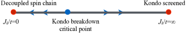
Figure 1: Renormalization group flow of the Kondo coupling, $J_{k}$, for a spin-1/2 chain on a semimetallic substrate.

Model Hamiltionian: We consider a spin-1/2 Heisenberg chain on a semimetallic substrate:

$$\hat{H} = -t\sum_{\langle{\boldsymbol{i}},{\boldsymbol{j}}\rangle,\sigma}\Big{(}e^{\frac{2\pi i}{\Phi_{0}}\int^{\boldsymbol{j}}_{\boldsymbol{i}}\boldsymbol{A}.\boldsymbol{d{\boldsymbol{l}}}}~{}\hat{\boldsymbol{c}}^{\dagger}_{{\boldsymbol{i}}}\hat{\boldsymbol{c}}_{{\boldsymbol{j}}}+h.c.\Big{)}$$ (1)

$$+\frac{J_{k}}{2}\sum^{L}_{\boldsymbol{l}=1}\hat{\boldsymbol{c}}^{\dagger}_{\boldsymbol{l}}\boldsymbol{\sigma}\hat{\boldsymbol{c}}_{\boldsymbol{l}}\cdot\hat{\boldsymbol{S}}_{\boldsymbol{l}}+J_{h}\sum^{L}_{\boldsymbol{l}=1}\hat{\boldsymbol{S}}_{\boldsymbol{l}}\cdot\hat{\boldsymbol{S}}_{\boldsymbol{l}+\Delta\boldsymbol{l}}.$$

Here, $t$ is the hopping parameter of the conduction electrons, the summation $\sum_{\langle{\boldsymbol{i}},{\boldsymbol{j}}\rangle}$ runs over a square lattice and $\hat{\boldsymbol{c}}^{\dagger}_{\boldsymbol{i}}=\big{(}\hat{c}^{\dagger}_{\boldsymbol{i},\uparrow},\hat{c}^{\dagger}_{\boldsymbol{i},\downarrow}\big{)}$ is a spinor where $\hat{c}^{\dagger}_{\boldsymbol{i},\uparrow(\downarrow)}$ creates an electron at site $\boldsymbol{i}$ with $z$-component of spin $1/2$ ($-1/2$). We use the Landau gauge, $\boldsymbol{A}=B(-y,0,0)$, and tune $B$ such that half a flux quantum ($\pi$-flux) pierces each plaquette. This gauge choice allows for translation symmetry by one lattice site in the $x$-direction. $J_{k}>0$ is the antiferromagnetic Kondo coupling between magnetic adatoms and conduction electrons, $J_{h}>0$ the Heisenberg coupling between magnetic adatoms, $L$ the length of the Heisenberg chain and linear length of the square conduction electron lattice, and $\hat{\boldsymbol{S}}_{\boldsymbol{l}}$ represents the spin-1/2 operators. We use an array of adatoms at interatomic distance $\Delta\boldsymbol{l}=(1,0)$ on the substrate and choose periodic boundary conditions along the spin chain and on the substrate to access the thermodynamic limit.

RG analysis: Consider the Hamiltonian in Eq. (1) at $J_{k}=0$. At low energies, this describes two decoupled conformal field theories (CFT): a (2+1)-D CFT corresponding to Dirac fermions, and a (1+1)-D CFT corresponding to SU(2)₁ WZW description of the spin-1/2 Heisenberg chain (we ignore the marginal perturbations that lead to multiplicative logarithmic corrections to the power-law correlations in the chain). The scaling dimension of Dirac fermions in $d$ space dimensions reads $\Delta_{\psi}=\frac{d}{2}$ and for the spin-1/2 chain, $\Delta_{S}=\frac{1}{2}$. At this decoupled fixed point, the Kondo coupling has a scaling dimension $2-2\Delta_{\psi}-\Delta_{S}=2-d-\frac{1}{2}=-\frac{1}{2}$ and is thereby irrelevant. On the other hand, in the limit $J_{k}\rightarrow\infty$ each spin-1/2 degree of freedom binds in a singlet with a conduction electron. This one-dimensional singlet product state, corresponding to the strong-coupling limit of the one-dimensional Kondo lattice model [Tsunetsugu et al., 1997], decouples from the conduction electrons, and effectively changes the boundary condition in the $y$-direction from periodic to open. At large but finite $J_{k}$, we expect the system to be locally described by a heavy Fermi liquid. Assuming these two regimes are separated by a single phase transition motivates us to find a suitable renormalization group (RG) description of the critical point separating the two regimes. The approach we follow is to consider $(d+1)$-dimensional Dirac fermions coupled to (1+1)-D Heisenberg chain. By power-counting, the Kondo coupling is marginal in $d=3/2$, which allows for an expansion in $\epsilon=d-3/2$, where the physical case of interest corresponds to $d=2$, i.e., $\epsilon=1/2$. Perturbing around the $J_{k}=0$ fixed point, the RG flow of dimensionless Kondo coupling $j_{k}=J_{k}\Lambda^{\epsilon}$ is given by:

$$\frac{dj_{k}}{d\ln\Lambda}=\epsilon j_{k}-\frac{j_{k}^{2}}{2}$$ (2)

where $\Lambda$ is an ultraviolet cutoff, and we have kept terms to $O(j_{k}^{2})$ (see Sec. I of Ref. [sup, ] for details). The resulting flow diagram is shown in Fig. 1 and the Kondo-breakdown critical fixed point is given by $j^{c}_{k}=2\epsilon$, which yields the correlation length exponent $\nu=1/\epsilon$. Due to Lorentz invariance, the critical theory will exhibit $\omega/T$ scaling in all observables.

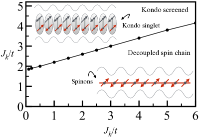
Figure 2: The zero-temperature mean-field phase diagram in a parameter space of $J_{k}/t$ and $J_{h}/t$. The critical line with symbols separates the two phases.

Large-N approximation: To formulate the large-N approximation, we use a fermion representation of the spin degree of freedom, $\boldsymbol{\hat{S}}_{\boldsymbol{l}}=\frac{1}{2}\hat{d}^{\dagger}_{\boldsymbol{l}}\boldsymbol{\sigma}\hat{d}_{\boldsymbol{l}}$ and impose the constraint $\boldsymbol{\hat{d}}^{\dagger}_{\boldsymbol{l}}\boldsymbol{\hat{d}}_{\boldsymbol{l}}=1$ with $\boldsymbol{\hat{d}}^{\dagger}_{\boldsymbol{l}}=\big{(}\hat{d}^{\dagger}_{\boldsymbol{l},\uparrow},\hat{d}^{\dagger}_{\boldsymbol{l},\downarrow}\big{)}$. The interaction part of the Hamiltonian can then be written as: $-\frac{J_{k}}{4}\sum_{\boldsymbol{l}}\big{(}\boldsymbol{\hat{c}}^{\dagger}_{\boldsymbol{l}}\boldsymbol{\hat{d}}_{\boldsymbol{l}}+h.c.\big{)}^{2}-\frac{J_{h}}{4}\sum_{\boldsymbol{l}}\big{(}\boldsymbol{\hat{d}}^{\dagger}_{\boldsymbol{l}}\boldsymbol{\hat{d}}_{\boldsymbol{l}+\Delta\boldsymbol{l}}+h.c.\big{)}^{2}+\frac{U}{2}\sum_{\boldsymbol{l}}\big{(}\boldsymbol{\hat{d}}^{\dagger}_{\boldsymbol{l}}\boldsymbol{\hat{d}}_{\boldsymbol{l}}-1\big{)}^{2}$. We now let the spin-index run from 1 to $N$, and take $N$ to infinity, which allows us to obtain the phase diagram in Fig. 2 using the saddle-point approximation. The saddle-point variables are determined by: $V=\sum_{\sigma}\langle\hat{c}^{\dagger}_{l,0,\sigma}\hat{d}_{l,0,\sigma}\rangle$, $\chi=\sum_{\sigma}\langle\hat{d}^{\dagger}_{l,\sigma}\hat{d}_{l+1,\sigma}\rangle$ and $\sum_{\sigma}\langle\hat{d}^{\dagger}_{l,\sigma}\hat{d}_{l,\sigma}\rangle=1$. The details of the calculations are presented in Secs. II and III of Ref. [sup, ]. Within this approximation, Kondo breakdown corresponds to the solution $V=0$ and $\chi\neq 0$ and Kondo screening to $V\neq 0$ and $\chi\neq 0$. As apparent, for each value of $J_{h}$ the mean-field solution shows a single transition. In the limit $J_{h}=0$, the critical value of $J_{k}$ corresponds to that of the single-impurity pseudogap Kondo problem. Aside from the mean-field order parameters, the transition can be detected by considering the spin-spin correlations along the chain. In the decoupled phase spinons are confined to chain and the spin-spin correlations – at the mean-field level – decay as $1/r^{2}$. In the Kondo-screened phase, spins hybridize with the Dirac electrons. Since the spin system is sub-extensive, the properties of the Dirac electrons remain unchanged and the spin-spin correlations along the chain inherit the 2D Dirac $1/r^{4}$ decay (see Fig. S3 of Ref. [sup, ]). Introducing particle-hole asymmetry by adding next-nearest hopping (while keeping a half-filled semimetallic state) was found to lead to similar results within large-N [sup, ].

QMC simulations: We have used the Algorithms for Lattice Fermions (ALF) [Bercx et al., 2017] implementation of the finite-temperature auxiliary-field QMC algorithm [Blankenbecler et al., 1981; White et al., 1989; Assaad and Evertz, 2008]. The perfect square form of the interaction used to formulate the large-N calculation complies with the standards of the ALF-library and the model can be readily implemented by decoupling the perfect square terms with a Hubbard Stratonovich transformation. The absence of negative sign problem follows by first carrying out a partial particle-transformation, $\hat{d}^{\dagger}_{\boldsymbol{l},\uparrow}\rightarrow e^{i\boldsymbol{Q}\cdot\boldsymbol{l}}\hat{d}_{\boldsymbol{l},\uparrow}$, and $\hat{c}^{\dagger}_{\boldsymbol{l},\uparrow}\rightarrow-e^{i\boldsymbol{Q}\cdot\boldsymbol{l}}\hat{c}_{\boldsymbol{l},\uparrow}$, and then using time reversal symmetry to prove that the eigenvalues of the fermion matrix occur in complex conjugate pairs. For a given system of linear length $L$, the QMC simulations are performed at an inverse temperature $\beta(=1/k_{B}T)=L$ and at a fix $J_{h}/t=1$. At $L=20$ we checked that the the choice $\beta=2L$ shows similar results as $\beta=L$. For the considered periodic boundary conditions, $L=4n+2$ corresponds to open-shell configurations and is known to show less finite-size effects than $L=4n+4$ sized systems.

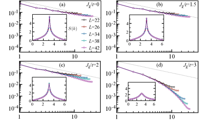
Figure 3: Equal-time spin-spin correlation function, $C(r)$, as a function of distance $r$ along the spin chain on a log-log scale for various values of $J_{k}/t$ at $J_{h}/t=1$ and $L_{x}=L_{y}=L=\beta$. The grey dashed line corresponds to $1/r$ decay and the corresponding static spin structure factors $S(k)$ are shown in the insets.

QMC results: Fig. 3 plots the spin-spin correlations $C(r)=4\langle{\hat{S}^{z}}_{0}{\hat{S}^{z}}_{r}\rangle$ as a function of distance $r$ for various values of $J_{k}/t$. In the limit of vanishing Kondo coupling, our results are consistent with the exact asymptotic form: $C(r)\propto(-1)^{r}\sqrt{\ln r}/r$. The $1/r$ decay of the spin-spin correlations in the Heisenberg model, is tied to SU(2) spin symmetry. If the Kondo coupling is irrelevant, then we expect $\sum_{\boldsymbol{l}}\hat{\boldsymbol{S}}_{\boldsymbol{l}}$ to remain a good quantum number of the low-energy effective theory. Thereby the asymptotic form of the spin-spin correlations should equally follow a $(-1)^{r}/r$ form. Remarkably, the data supports this point of view up to $J_{k}/t\lesssim 2$. On the other hand, in the Kondo-screened phase for $J_{k}/t\gtrsim 2$, the equal-time correlations decay with a power larger than unity. In this phase, we expect the spin-spin correlations to inherit the power-law of the Dirac fermions $\langle{\hat{S}^{z,c}}_{\boldsymbol{l}}{\hat{S}^{z,c}}_{\boldsymbol{l}+{\boldsymbol{r}}}\rangle\propto 1/r^{4}$. (see Fig. S3 of Ref. [sup, ]). The insets of Fig. 3 plot the static spin structure factor $S(k)=\frac{1}{L}\sum_{r}e^{-ik\cdot r}C(r)$ as a function of momentum $k$. Noticeably, both at $J_{k}=0$ and $J_{k}/t=1.5$ we observe systematic growth of $S(k)$ at $k=\pi$, reflecting the $(-1)^{r}/r$ real space decay. At $J_{k}/t=2$ we observe a cusp feature but a saturation of $S(k=\pi)$ with system size thus suggesting a power law with exponent $1<K_{\sigma}<2$. Finally, in the Kondo-screened phase at $J_{k}/t=3$, $S(k)$ converges to a smooth function implying $K_{\sigma}>2$. A detailed overview of the QMC data is given in Sec. IV of Ref. [sup, ].

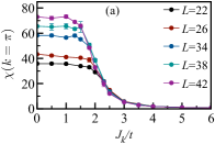
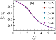
Figure 4: Left: Magnetic susceptibility $\chi(k=\pi)$ as a function of $J_{k}/t$ for $J_{h}/t=1$ and $\beta=L$. Right: Plots $\partial F/\partial J_{k}$ as a function of $J_{k}/t$.

To confirm the above, we have computed the spin susceptibility $\chi(k)=\int_{0}^{\beta}d\tau S(k,\tau)$ with $S(k,\tau)$ given as:

$$S(k,\tau)=\sum_{r}e^{-ik\cdot r}\langle S^{z}(r,\tau)S^{z}(r=0,\tau=0)\rangle.$$ (3)

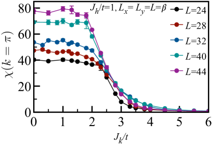
Figure S8: Magnetic susceptibility, $\chi(k=\pi)$, as a function of $J_{k}/t$ for different system size at $\beta=L$ on $4n+4$ lengths chain.

Lorentz invariance, inherent to spin chains, renders space and time interchangeable such that the time displaced correlation function scales as $1/\sqrt{r^{2}+(v_{s}\tau)^{2}}$ with $v_{s}$ the spin velocity. Setting $\beta=L$, we hence expect $\chi(k=\pi)$ to diverge as $L$. Fig. 4 (a) plots $\chi(k=\pi)$ at $\beta=L=4n+2$. A similar data at $L=4n+4$ can be found in Fig. S8 of Ref. [sup, ]. For both cases we see two phases, one in which $\chi(k=\pi)$ scales as $L$ and one in which it scales to a $L$-independent constant. In Fig. 4 (b) we plot $\frac{1}{L}\frac{\partial F}{\partial J_{k}}=\frac{2}{3L}\sum^{L}_{\boldsymbol{l}=1}\langle\hat{\boldsymbol{c}}^{\dagger}_{\boldsymbol{l}}\boldsymbol{\sigma}\hat{\boldsymbol{c}}_{\boldsymbol{l}}\cdot\hat{\boldsymbol{S}}_{\boldsymbol{l}}\rangle$ so as to inquire the nature of the transition. The data favors a smooth curve, and hence a continuous quantum phase transition.

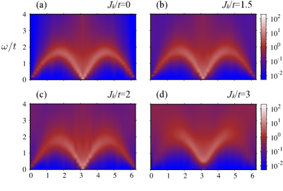
Figure 5: Dynamical spin structure factor, $S(k,\omega)$, along spin chain as a function of energy ($\omega/t$) and momentum ($k$) for $L=\beta=44$ at $J_{h}/t=1$.

We now consider the dynamical spin structure factor, that relates to the imaginary-time correlation functions through $S(k,\tau)=\frac{1}{\pi}\int d\omega~{}\frac{e^{-\tau\omega}}{1-e^{-\beta\omega}}~{}\chi^{\prime\prime}(k,\omega)$. To extract $S(k,\omega)=\frac{\chi^{\prime\prime}(k,\omega)}{1-e^{-\beta\omega}}$, we use the ALF-implementation of the stochastic analytical continuation algorithm [Beach, 2004]. The excitation spectrum of the isolated spin-1/2 Heisenberg chain is well understood and consists of a two-spinon continuum bounded by $\frac{\pi}{2}J_{h}\sin(k)\leq\omega(k)\leq\pi J_{h}\sin\left(\frac{k}{2}\right)$. Fig. 5 plots the dynamical spin spectral function for different values of $J_{k}/t$. Remarkably, the spin dynamics of the Heisenberg chain remains unaffected by conduction electron for $J_{k}/t\lesssim 2$. In the screened phase at $J_{k}/t>2$ spinons bind and low-energy spectral weight is depleted.

Figure 6: Conduction-electron spectral function, $A_{0}(k,\omega)$, as a function of energy ($\omega/t$) and momentum ($k$) on $L=\beta=44$ lattice at $J_{h}/t=1$.

In Kondo lattices, a Kondo-breakdown transition implies an abrupt change of the Luttinger volume. In our setup such a notion cannot be applied since the localized spin-1/2 moments are sub-extensive. Nevertheless, we can consider the spectral function of the conduction electrons that directly couple to the localized spin-1/2 moments and investigate how it evolves across the transition. Let $A_{n}(k,\omega)=-\frac{1}{\pi}\text{Im}G^{\text{ret}}_{n}(k,\omega)$ with $G^{\text{ret}}_{n}(k,\omega)=-i\int_{0}^{\infty}dte^{i\omega t}\sum_{\sigma}\langle\{\hat{c}_{k,n,\sigma}(0),\hat{c}^{\dagger}_{k,n,\sigma}(t)\}\rangle$. In the considered Landau gauge, translation symmetry is present along the $x$-direction and $\hat{c}_{k,n,\sigma}=\frac{1}{\sqrt{L}}\sum_{m=1}^{L}e^{ikm}\hat{c}_{\boldsymbol{i}=(m,n),\sigma}$ is the partial Fourier transform. Fig. 6 plots $A_{0}(k,\omega)$ corresponding to the conduction electrons that couple to the Heisenberg chain. At $J_{k}=0$ the spectral function shows a dominant $\epsilon(k)=2t\cos(ka)$ dispersion. In the Kondo-breakdown phase and even at relatively large values of $J_{k}/t=1.5$ we observe no signs of hybridization with the spins. In contrast in the Kondo-screened phase, $J_{k}/t\gtrsim 2$, a clear signature of hybridization is apparent.

STM experiments of magnetic adatoms on metallic surfaces, separated by an insulating buffer layer shown in Ref. [Spinelli et al., 2015, Toskovic et al., 2016], measure tunneling between tip and substrate occurring through the localized orbitals. In our setup we can access this quantity by carrying out a Schrieffer-Wolff transformation of the localized electron creation operator in the realm of the Anderson model [Danu et al., 2019, Raczkowski and Assaad, 2019, Costi, 2000]. In particular, $A_{\boldsymbol{l}}(\omega)=-\text{Im}G_{\boldsymbol{l}}^{\text{ret}}(\omega)$ with $G_{\boldsymbol{l}}^{\text{ret}}(\omega)=-i\int_{0}^{\infty}dte^{i\omega t}\sum_{\sigma}\big{<}\big{\{}\tilde{c}_{\boldsymbol{l},\sigma}(t),\tilde{c}_{\boldsymbol{l},\sigma}^{\dagger}(0)\big{\}}\big{>}$ and $\tilde{c}_{\boldsymbol{l},\sigma}^{\dagger}=\hat{c}^{\dagger}_{\boldsymbol{l},-\sigma}\hat{S}^{\sigma}_{\boldsymbol{l}}+\sigma\hat{c}_{\boldsymbol{l},\sigma}^{\dagger}\hat{S}^{z}_{\boldsymbol{l}}$. Here $\sigma=\pm$ runs over the two spin polarizations and $\hat{S}^{\pm}_{\boldsymbol{l}}=\hat{S}^{x}_{\boldsymbol{l}}\pm i\hat{S}^{y}_{\boldsymbol{l}}$. To evaluate the zero-bias tunneling signal we estimate $A_{\boldsymbol{l}}(\omega=0)\simeq\frac{1}{\pi}\beta G_{\boldsymbol{l}}(\tau=\beta/2)$. Fig. 7 plots this quantity. Remarkably, in the Kondo-breakdown phase, we are not able to distinguish the signal from zero. This supports the notion that spins and conduction electrons decouple at low energies. As $J_{k}\rightarrow\infty$ the spin binds in a singlet with the conduction electron and the tunneling signal through the adatom drops. A more detailed numerical analysis [Luitz et al., 2012, Karrasch et al., 2010] of the STM signal across the transition is certainly of great interest.

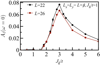
Figure 7: Zero-bias tunneling through the magnetic adatom.

Conclusion: We have shown that a one-dimensional spin chain coupled via a Kondo interaction to 2D Dirac fermions provides a realization of a continuous Kondo-breakdown transition. Weak coupling $J_{k}$ is irrelevant and gapless spinons exist while propagating along the one-dimensional chain. The reason for the absence of Kondo screening in this phase is qualitatively similar to its absence at deconfined quantum critical points in 2D [Grover and Senthil, 2010]: in both cases, the anomalous dimension of the spin operator is ‘large’ due to fractionalization, which makes conduction electrons ineffectual at Kondo screening. Beyond the transition, Kondo screening appears and gapless spinons bind. The Kondo-screened phase is adiabatically connected to the strong-coupling limit, where each spin binds with a conduction electron into a spin singlet. Larger systems will be needed to determine the critical exponents such as the anomalous dimension of the local moments. In addition, since the number of adatoms in experiments is tunable [Toskovic et al., 2016; Choi et al., 2017; Moro-Lagares et al., 2019], it will be very useful to determine how many of them are needed to resolve Kondo breakdown in an interacting spin chain.

The choice of Dirac fermions which only possess Fermi points simplifies the problem and allows for an RG analysis. This is in contrast to the conventional Hertz-Millis-Moriya approach [Hertz, 1976; Millis, 1993; Moriya, 2012] where one integrates out the fermions to obtain an effective non-local action for local moments. Indeed, past work on Fermi surface coupled to a spin-chain employed Hertz-Millis-Moriya approach, and concluded that the Kondo interaction is relevant (marginal) for an $XXZ$ (Heisenberg) chain, thus destabilizing the Luttinger liquid for infinitesimal Kondo coupling [Lobos et al., 2012]. In our problem, the irrelevancy of the Kondo interaction at the decoupled fixed point ($J_{k}=0$) continues to hold even for a U(1) symmetric $XXZ$ spin-chain and we expect that the qualitative features of our phase diagram will remain unchanged. It will be desirable to study the problem of Fermi surface coupled to an $XXZ$ chain using QMC method, which would also help bridge the gap with experiments in Refs. [Spinelli et al., 2015; Toskovic et al., 2016; Choi et al., 2017; Moro-Lagares et al., 2019; Bork et al., 2011; Zhou et al., 2010; Serrate et al., 2010]. In addition, other scenarios for Kondo breakdown, such as the one discussed in Ref. [Komijani and Coleman, 2019], can also be studied using QMC.

In summary, we studied a problem of spin-chain coupled to Dirac fermions and established a Kondo breakdown transition using a combination of techniques. Our results open the window to design and inform new experiments, along the lines of Refs. [Toskovic et al., 2016; Choi et al., 2017; Moro-Lagares et al., 2019], where adatoms can be suitably arranged on metal/semimetal surfaces.

Acknowledgments: The authors thank M. Aronson, T.-C. Lu, J. McGreevy for useful conversations, and F. Mila for insightful collaborations on a related subject. The authors gratefully acknowledge the Gauss Centre for Supercomputing e.V. (www.gauss-centre.eu) for providing computing time on the GCS Supercomputer SUPERMUC-NG at Leibniz Supercomputing Centre (www.lrz.de). The research has been supported by the Deutsche Forschungsgemeinschaft through grant number AS 120/14-1 (FFA), the Würzburg-Dresden Cluster of Excellence on Complexity and Topology in Quantum Matter - ct.qmat (EXC 2147, project-id 39085490) (FFA and MV), and SFB 1143 (project-id 247310070) (MV). TG is supported by the National Science Foundation under Grant No. DMR-1752417, and as an Alfred P. Sloan Research Fellow. FFA and TG thank the BaCaTeC for partial financial support.

I Details of Renormalization Group analysis

The perturbative RG flow close to the $J_{k}=0$ fixed point can be obtained via operator product expansion (OPE). We consider Dirac fermions in $d+1$ dimensions coupled to a (1+1)-D spin-1/2 Heisenberg chain. Although the low-energy theory of the Heisenberg chain is not a pure CFT due to marginal operators, we neglect the effect of these operators, and assume that the chain is described by a 1+1-D SU(2)₁ WZW model. Thus, the low-energy imaginary-time action is given by:

$$\mathcal{S}=\mathcal{S}_{\textrm{WZW}}+\int d^{d}xd\tau\,\,\overline{\psi}\not{p}\psi+J_{k}\int dxd\tau\,\,\hat{\boldsymbol{c}}^{\dagger}(x,\tau)\frac{\boldsymbol{\sigma}}{2}\hat{\boldsymbol{c}}(x,\tau)\cdot\hat{\boldsymbol{S}}(x,\tau)$$ (S1)

where $\mathcal{S}_{\textrm{WZW}}$ is the WZW action for the Heisenberg chain. The crucial observation is that the tree-level scaling dimension of the operator corresponding to Kondo interaction, $O_{J_{k}}=\hat{\boldsymbol{c}}^{\dagger}(x,\tau)\frac{\boldsymbol{\sigma}}{2}\hat{\boldsymbol{c}}(x,\tau)\cdot\hat{\boldsymbol{S}}(x,\tau)$ is $\Delta^{0}_{J_{k}}=\epsilon$, where $\epsilon=d+1/2-2=d-3/2$. This allows for a perturbative access to a UV critical point which becomes unstable towards a stable phase where Kondo interaction is irrelevant (see Fig. 1). Defining a dimensionless Kondo coupling $j_{k}=J_{k}\Lambda^{\epsilon}$, where $\Lambda$ is a UV cut-off scale, the OPE of this operator with itself is given by:

$$:O_{j_{k}}::O_{j_{k}}:=c\hat{\mathbf{1}}+:O^{2}_{j_{k}}:=c\hat{\mathbf{1}}-\frac{1}{2}:O_{j_{k}}:$$ (S2)

where $:\,:$ denotes normal ordering, $c$ is a constant and $\hat{\mathbf{1}}$ denotes the identity operator. The above equation implies that the OPE expansion coefficient $c_{j_{k}j_{k}j_{k}}=-1/2$ and thus the RG flow equation upto $O(j_{k}^{2})$ is given by:

$$\frac{dj_{k}}{d\ln\Lambda}=\epsilon j_{k}-\frac{j^{2}_{k}}{2}.$$ (S3)

II Auxiliary-field path integral and saddle-point approximation

We consider SU(N) generalization of the model presented in Eq.(blue1) of the main text:

$$\hat{H} = \hat{H}_{t}-\frac{J_{k}}{4N}\sum_{\boldsymbol{l}}\Big{\{}\big{(}\boldsymbol{\hat{c}}^{\dagger}_{\boldsymbol{l}}\boldsymbol{\hat{d}}_{\boldsymbol{l}}+h.c.\big{)}^{2}+\big{(}i\boldsymbol{\hat{c}}^{\dagger}_{\boldsymbol{l}}\boldsymbol{\hat{d}}_{\boldsymbol{l}}+h.c.\big{)}^{2}\Big{\}}$$ (S4)

$$-\frac{J_{h}}{4N}\sum_{\boldsymbol{l}}\Big{\{}\big{(}\boldsymbol{\hat{d}}^{\dagger}_{\boldsymbol{l}}\boldsymbol{\hat{d}}_{\boldsymbol{l}+\Delta\boldsymbol{l}}+h.c.\big{)}^{2}+\big{(}i\boldsymbol{\hat{d}}^{\dagger}_{\boldsymbol{l}}\boldsymbol{\hat{d}}_{\boldsymbol{l}+\Delta\boldsymbol{l}}+h.c.\big{)}^{2}\Big{\}}+\frac{U}{N}\sum_{\boldsymbol{l}}\big{(}\boldsymbol{\hat{d}}^{\dagger}_{\boldsymbol{l}}\boldsymbol{\hat{d}}_{\boldsymbol{l}}-1\big{)}^{2}$$

where $\boldsymbol{\hat{d}}^{\dagger}_{\boldsymbol{l}}$ is now an $N$ component fermion (see Ref. [Raczkowski and Assaad, 2020]). Note that since our Monte Carlo simulations are restricted to SU(2) we can omit the perfect square terms of the current operator [Assaad, 1999, Capponi and Assaad, 2001]. We will however pursue this discussion for a general value of $N$ so as to be able to derive the saddle-point equations in the large-N limit.

Using the Hubbard-Stratonovich (HS) transformation the partition function can be written as:

$$Z~{}\equiv~{}\int\mathcal{D}\{\mathcal{V},\mathcal{\chi},\mathcal{\lambda}\}~{}e^{-N\mathcal{S}\{\mathcal{V},\mathcal{\chi},\mathcal{\lambda}\}}$$ (S5)

with the action

$$\mathcal{S}\{\mathcal{V},\mathcal{\chi},\lambda\}=-\ln\Big{[}~{}\mbox{Tr}~{}\mathcal{T}e^{-\int^{\beta}_{0}d\tau~{}\hat{H}\{\mathcal{V},\mathcal{\chi},\lambda\}}\Big{]}+\int^{\beta}_{0}d\tau\sum_{\boldsymbol{l}}\Big{\{}\frac{J_{k}}{4}|\mathcal{V}(\boldsymbol{l},\tau)|^{2}+\frac{J_{h}}{4}|\mathcal{\chi}(\boldsymbol{l},\tau)|^{2}+\frac{U}{4}|\lambda(\boldsymbol{l},\tau)|^{2}\Big{\}}$$ (S6)

and time dependent Hamiltonian

$$\hat{H}\{\mathcal{V},\mathcal{\chi},\lambda\}=\hat{H}_{t}+\sum_{\boldsymbol{l}}\Big{\{}-\frac{J_{k}}{2}\big{(}\mathcal{V}(\boldsymbol{l},\tau)\boldsymbol{\hat{c}}^{\dagger}_{\boldsymbol{l}}\boldsymbol{\hat{d}}_{\boldsymbol{l}}+h.c\big{)}-\frac{J_{h}}{2}\big{(}\mathcal{\chi}(\boldsymbol{l},\tau)\boldsymbol{\hat{d}}^{\dagger}_{\boldsymbol{l}}\boldsymbol{\hat{d}}_{\boldsymbol{l}+\Delta\boldsymbol{l}}+h.c\big{)}-iU\lambda(\boldsymbol{l},\tau)\big{(}\boldsymbol{\hat{d}}^{\dagger}_{\boldsymbol{l}}\boldsymbol{\hat{d}}_{\boldsymbol{l}}-1\big{)}\Big{\}}.$$ (S7)

Here, the scalar Lagrange multiplier $\mathcal{\lambda}(\boldsymbol{l},\tau)$ enforces the constraint and $\mathcal{V(\boldsymbol{l},\tau)}$ and $\mathcal{\chi(\boldsymbol{l},\tau)}$ are complex bond fields. In the QMC simulations we sum over all field configurations to obtain an exact result. At the particle-hole symmetric point, and as argued in the main text, the imaginary part of the action takes the value $n\pi$ with $n$ an integer. Hence for even values of $N$ no negative sign problem occurs.

In the large-N limit, we expect the saddle-point approximation to become exact:

$$\frac{d\mathcal{S}\{\mathcal{V},\mathcal{\chi},\mathcal{\lambda}\}}{d\mathcal{V}(\boldsymbol{l},\tau)},\frac{d\mathcal{S}\{\mathcal{V^{*}},\mathcal{\chi^{*}},\lambda\}}{d\mathcal{V}^{*}(\boldsymbol{l},\tau)}=0,\quad\mbox{and},\quad\frac{d\mathcal{S}\{\mathcal{V},\mathcal{\chi},\mathcal{\lambda}\}}{d\mathcal{\chi}(\boldsymbol{l},\tau)},\frac{d\mathcal{S}\{\mathcal{V^{*}},\mathcal{\chi^{*}},\mathcal{\lambda}\}}{d\mathcal{\chi}^{*}(\boldsymbol{l},\tau)}=0,\quad\mbox{and},\quad\frac{d\mathcal{S}\{\mathcal{V},\mathcal{\chi},\mathcal{\lambda}\}}{d\mathcal{\lambda}(\boldsymbol{l},\tau)}=0.$$ (S8)

In the mean-field approximation carried out in the next sections, we restrict the search for saddle points to space and time independent fields: $\mathcal{V}(\boldsymbol{l},\tau)=\mathcal{V}^{*}(\boldsymbol{l},\tau)=V(\in R)$ and $\mathcal{\chi}(\boldsymbol{l},\tau)=\mathcal{\chi}^{*}(\boldsymbol{l},\tau)=\chi(\in R)$ and impose the constraint only on average.

III Large-N mean field calculation for a chain of magnetic adatoms

We consider an infinite Heisenberg chain of adatoms with periodic boundary conditions. The unit cell, denoted as $l$, contains $n\in\left[1\cdots N_{c}\right]$ conduction electrons $\hat{c}_{l,n,\sigma}$ and a single spin degree of freedom. In this case the mean-field Hamiltonian can be written as,

$$\hat{H}_{mf}= \sum_{k,\sigma,n,n^{\prime}}\hat{c}^{\dagger}_{k,n,\sigma}T(k)_{n,n^{\prime}}\hat{c}_{k,n^{\prime},\sigma}-\frac{J_{h}\chi}{2}\sum_{k,\sigma}{\epsilon}^{d}_{k}\hat{d}^{\dagger}_{k,\sigma}\hat{d}_{k,\sigma}+\lambda\sum_{k,\sigma}\hat{d}^{\dagger}_{k,\sigma}\hat{d}_{{k},\sigma}-\frac{J_{k}V}{2}\sum_{k,\sigma}(\hat{c}^{\dagger}_{k,1,\sigma}\hat{d}_{k,\sigma}+h.c)+e_{0}N_{u}$$ (S9)

where, ${\epsilon}^{d}_{k}=2\cos(ka)$, $e_{0}=(\frac{J_{k}V^{2}}{2}+\frac{J_{h}\chi^{2}}{2}-\lambda+\mu)$ and $N_{u}$ is the number of unit cells. Hereafter, we will set $a=1$. The mean-field order parameters are defined as $V=\sum_{\sigma}\langle\hat{c}^{\dagger}_{l,1,\sigma}\hat{d}_{l,\sigma}\rangle=\sum_{\sigma}\langle\hat{d}^{\dagger}_{l,\sigma}\hat{c}_{l,1,\sigma}\rangle$, $\chi=\sum_{\sigma}\langle\hat{d}^{\dagger}_{l+1,\sigma}\hat{d}_{l,\sigma}\rangle=\sum_{\sigma}\langle\hat{d}^{\dagger}_{l,\sigma}\hat{d}_{l+1,\sigma}\rangle$, and, the Lagrange multiplier $\lambda$ will enforce the constraint $\sum_{\sigma}\langle\hat{d}^{\dagger}_{l,\sigma}\hat{d}_{l,\sigma}\rangle=1$ on average. The mean field Hamiltonian is then given by:

$$\hat{H}_{mf}=\sum_{k,\sigma}\hat{\boldsymbol{\phi}}^{\dagger}_{k,\sigma}M(k)\hat{\boldsymbol{\phi}}_{k,\sigma}+N_{u}e_{0}$$ (S10)

with $\boldsymbol{\hat{\phi}}^{\dagger}_{k,\sigma}=\left(\hat{c}^{\dagger}_{k,1,\sigma},\cdots,\hat{c}^{\dagger}_{k,N_{c},\sigma},\hat{d}^{\dagger}_{k,\sigma}\right)$ and

$$M(k)=$$

$$\left(\begin{array}[]{cccccccccccccccc}-2t\cos k-\mu&~{}~{}-t-2t^{\prime}\cos k&0&0&0&\cdots&\cdots&~{}-t-2t^{\prime}\cos k&-\frac{J_{k}V}{2}\\ -t-2t^{\prime}\cos k&~{}~{}2t\cos k-\mu&~{}~{}-t-2t^{\prime}\cos k&0&0&\cdots&\cdots&0&0\\ 0&~{}~{}-t-2t^{\prime}\cos k&~{}~{}-2t\cos k-\mu&~{}~{}-t-2t^{\prime}\cos k&0&\cdots&\cdots&0&0\\ \cdots&\cdots&\cdots&\cdots&\cdots&\cdots&\cdots&\cdots&\cdots\\ \cdots&\cdots&\cdots&\cdots&\cdots&\cdots&\cdots&\cdots&\cdots\\ -t-2t^{\prime}\cos k{}{}&0&0&0&0&\cdots&\cdots&2t\cos k-\mu&0\\ \ -\frac{J_{k}V}{2}&0&0&0&0&\cdots&\cdots&0&-J_{h}\chi\cos k+\lambda\end{array}\right).$$

In the above we have added a next-nearest hopping $t^{\prime}$ term that lifts the particle-hole (ph) symmetry of the model. We will nevertheless consider the half-filled case. Diagonalising: $U^{\dagger}(k)M(k)U(k)=\text{Diag}\left(E_{k,1},\cdots,E_{k,N_{c}+1}\right)$ gives:

$$\hat{H}_{mf}=N_{u}e_{0}+\sum_{k,\sigma}\sum^{N_{c+1}}_{n=1}E_{k,n}{\hat{\psi}}^{\dagger}_{k,n,\sigma}{\hat{\psi}}_{k,n,\sigma}$$ (S12)

with $\boldsymbol{\hat{\psi}}^{\dagger}_{k,\sigma}=\boldsymbol{\hat{\phi}}^{\dagger}_{k,\sigma}U(k)$.

The ground state energy per unit cell can be computed as

$$e_{g}=e_{0}+\frac{2}{N_{u}}\sum_{k}\sum^{N_{c+1}}_{n=1,E_{k,n}<0}E_{k,n}.$$ (S13)

The mean-field parameters $V$ and $\chi$ are obtained by minimizing the ground state energy ($e_{g}$) using the simplex method (see Ref. [Nelder and Mead, 1965]) in the constrained space $\sum_{\sigma}\langle\hat{d}^{\dagger}_{l,\sigma}\hat{d}_{l,\sigma}\rangle=1$ and total number of particles $L^{2}+L$. These constraints are imposed by adjusting $\mu$ and $\lambda$.

III.1 The particle-hole symmetric case

At $t^{\prime}=0$ both the chemical potential and Lagrange multiplier are pinned to zero due to particle-hole symmetry. The mean field values for $V$ and $\chi$ as a function of $J_{k}/t$ at fix $J_{h}/t=1$ are shown in Fig. S2 for $L=4n+4$ (see top panel) and for $L=4n+2$ (see bottom panel).

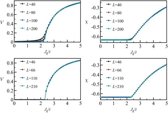
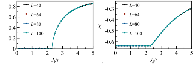
Figure S1: Top panel: Mean-field parameters $V$ and $\chi$ as a function of $J_{k}/t$ at $J_{h}/t=1$ on $4n+4$ lengths chain. Bottom panel: Mean-field parameter $V$ and $\chi$ as a function of $J_{k}/t$ at $J_{h}/t=1$ on $4n+2$ lengths chain. In both case the we have use periodic boundary condition along the spin chain direction as well in $y$-direction of the substrate.

Figure S2: Mean-field parameters $V$ and $\chi$ as a function of $J_{k}/t$ at $J_{h}/t=1$ for $L=4n+4$ with anti-periodic boundary condition.

For one dimensional systems, it is advantageous to adapt the boundary condition to the particle number so as to optimize extrapolation to the thermodynamic limit. In particular, anti-periodic (periodic) boundaries for systems with 4n+4 (4n + 2) guarantees that the non-interaction system has a unique ground state. As apparent in Figs. S2 (bottom) and S2, when these conditions are met, a quick scaling to the thermodynamic limit is obtained. If not (see Fig. S2 (top)) extrapolation to the thermodynamic limit is hard, but ultimately, the same results are obtained.

The mean-field results clearly show two phases upon tuning $J_{k}/t$ at fixed $J_{h}$. The decoupled phase is characterized by $V=0$, $\chi\neq 0$, and the Kondo-screened state by $V\neq 0$, $\chi\neq 0$. The mean-field phase diagram in the $J_{h}/t$ versus $J_{k}/t$ plane is shown in Fig. 2 of main text. The transition is continuous and, the mean-field Kondo breakdown critical point takes place at $J^{c}_{k}/t\approx 2.3$ for $J_{h}/t=1$.

In the decoupled phase, the spin-spin correlations, $C(r)=\frac{1}{L}\sum_{q}e^{-iq.r}\langle S^{z}(q)S^{z}(-q)\rangle$ decay as $1/r^{2}$ reflecting the scaling dimension $d/2$ with $d=1$ for the mean-field description of spinons. In the Kondo-screened phase we expect the spin-spin correlations along the chain to acquire the scaling behavior of the Dirac substrate, $1/r^{4}$. This expectation, that stems from the fact that the spin system is sub-extensive and hence cannot alter the properties of the substrate, is positively checked in Fig. S3.

Finally in Fig. S4 we plot $E_{k,n}$ in the decoupled and Kondo-screened phases. In the decoupled phase, $J_{k}/t=1.5$, we observe the spinon-band and the 2D Dirac electrons. With our gauge choice and periodic boundary conditions, the Dirac cones are located at $\boldsymbol{k}=\pm\left(\frac{\pi}{2},\frac{\pi}{2}\right)$. Furthermore, the Fermi velocity is set by $v_{F}=2t$ and the spinon velocity by $J_{h}\chi$. In the Kondo-screened phase at $J_{k}/t=3$ hybridization between spin and Dirac electrons is apparent. In the limit of large $J_{k}$ we observe bonding and anti-bonding bands of the spinon and conduction electrons $\hat{c}_{k,1,\sigma}$ that split off at low and high energy. In this limit, the Dirac electrons are subject to open boundary conditions in the $y$-direction. For the given cut, no edge states are expected.

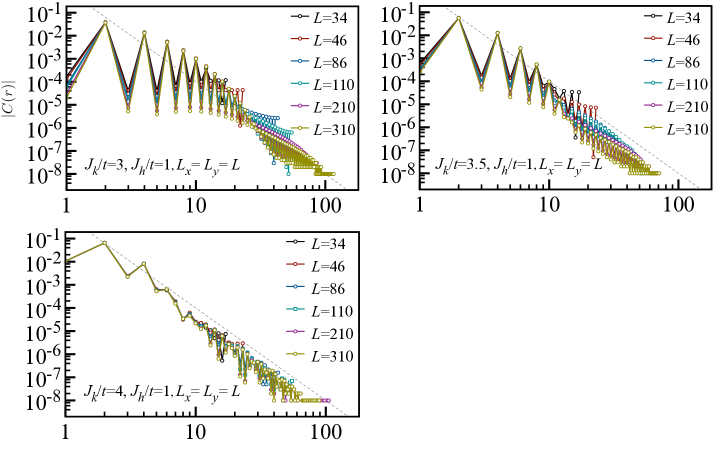
Figure S3: Log-log scale plots of equal time spin-spin correlation function $C(r)$ as a function of distance $r$ along the spin chain for the given $J_{k}/t$ values computed in large-N mean-field calculation. The grey dashed line corresponds to the $1/r^{4}$ form.

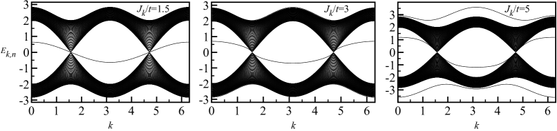
Figure S4: Band energies, $E_{k,n}$, as a function of momentum ($k$) for $J_{h}/t=1$ and $L_{x}=L_{y}=L=200$. Particularly, in the decoupled (left), Kondo-screened (center) and strong-coupling (right) phases. Here, particle-hole symmetry results in: $E_{k+\pi,n}=-E_{k,n^{\prime}}$ for a pair of bands $n,n^{\prime}$.

III.2 The particle-hole asymmetric case

In free standing graphene, particle-hole symmetry is an emergent symmetry. The question we will address here is if our results depend on the Hamiltonian being particle-hole symmetric. The breaking of this symmetry results in a negative sign problem in the QMC approach, such that we will answer this question in the realm of the large-N mean-field theory. Including a $t^{\prime}$ matrix element in our calculations breaks the particle-hole symmetry. Since the point group symmetry remains unchanged, the Dirac cones do not meander and remain pinned at $\boldsymbol{K}=\pm(\pi/2,\pi/2)$ for our Landau gauge choice.

The mean-field order parameters as well as the Lagrange multiplier are plotted in Fig. S6 for various values of $t^{\prime}$. Remarkably, the results remain next to unchained. To understand whay, it is instructive to analyze low-energy effective model for the Dirac electrons at finite $t^{\prime}$. The corresponding tight-binding Hamiltonian with a nearest ($t$) and the next-nearest neighbor ($t^{\prime}$) hopping on the square lattice on a torus, Landau gauge $\boldsymbol{A}=B(-y,0,0)$ with $Ba^{2}/\phi_{0}=1/2$, can be written as,

$$\hat{H}^{tt^{\prime}}=\sum_{\boldsymbol{k}}\big{(}\begin{array}[]{cccccccc}\hat{a}^{\dagger}_{\boldsymbol{k}},&\hat{b}^{\dagger}_{\boldsymbol{k}}\\ \end{array}\big{)}\left(\begin{array}[]{cccccccc}-2t\cos k_{x}&\underbrace{-t(1+e^{-i2k_{y}})-2t^{\prime}\cos k_{x}(1+e^{-2ik_{y}})}_{Z_{\boldsymbol{k}}}\\ \underbrace{-t(1+e^{i2k_{y}})-2t^{\prime}\cos k_{x}(1+e^{2ik_{y}})}_{Z^{*}_{\boldsymbol{k}}}&2t\cos k_{x}\end{array}\right)\left(\begin{array}[]{cccccccc}\hat{a}_{\boldsymbol{k}}\\ \hat{b}_{\boldsymbol{k}}\\ \end{array}\right).$$ (S18)

(S19)

In the above we have set $a=1$. The magnetic unit cell contains two orbitals with associated creation operators, $\hat{a}^{\dagger}_{{\boldsymbol{k}}}$ and $\hat{b}^{\dagger}_{{\boldsymbol{k}}}$, and the lattice vectors are given by $\boldsymbol{a}_{1}=(1,0)$, $\boldsymbol{a}_{2}=(0,2)$. The dispersion then reads:

$$\epsilon_{\pm}({\boldsymbol{k}})=\pm\sqrt{4t^{2}\cos^{2}k_{x}+|Z({\boldsymbol{k}})|^{2}}.$$ (S20)

By symmetry one will check that the Dirac points remain pinned at ${\boldsymbol{K}}=\pm\frac{\pi}{2}(1,1)$. Expansion around the Dirac points gives:

$$H^{tt^{\prime}}(\pm{\boldsymbol{K}}+{\boldsymbol{q}})\approx 2t\big{(}\pm\hat{\sigma}_{z}q_{x}-\hat{\sigma}_{y}q_{y}\big{)}\mp 4t^{\prime}q_{x}q_{y}\hat{\sigma}_{y}.$$ (S21)

As apparent in the low-energy limit, $t^{\prime}$, can be neglected since it comes in second order in $\boldsymbol{q}$. This explains the fact that our results, at least at weak coupling remain unchanged.

The band energies, $E_{k,n}$, as a function of momentum $k$ are shown in Fig. S6. Here, the particle hole asymmetry is apparent since the relation $E_{k+\pi,n}=-E_{k,n^{\prime}}$ does not hold for a pair of bands $n,n^{\prime}$.

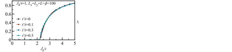
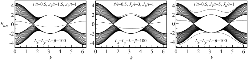
Figure S5: Mean-field parameters; $V$ (left), $\chi$ (center) and $\lambda$ (right), as a function of $J_{k}/t$ for the given parameters values.

Figure S6: Band energies, $E_{k,n}$, as a function of momentum ($k$) for the given parameters values. Particularly, in the decoupled (left), Kondo-screened (center) and strong-coupling (right) phases.

IV Details of QMC results

Here we provide additional QMC results.

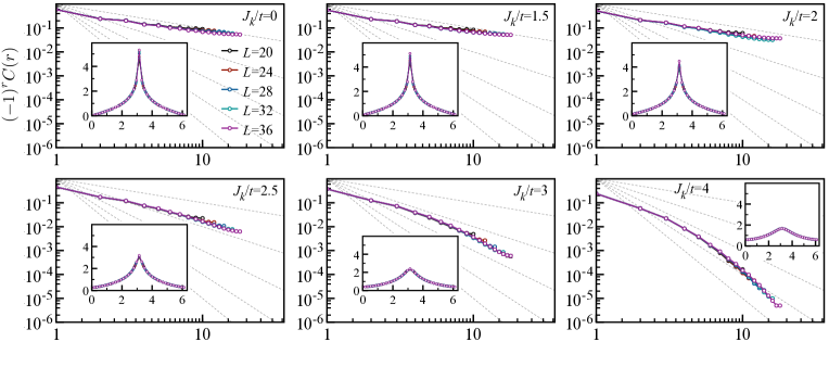
Figure S7: Equal time spin correlation function $C(r)$ as a function of distance $r$ in log-log scale for given values of $J_{k}/t$ on $4n+4$ lengths chain for $J_{h}//t=1$ and $L_{x}=L_{y}=L=\beta$. The corresponding static spin structure factors $S(k)$ as a function of momentum ($k$) are shown in subfigures. The grey dashed line denotes the $1/r^{n}$ with powers $n$ starting from $n=1$ (first line) to $n=5$ (last line).

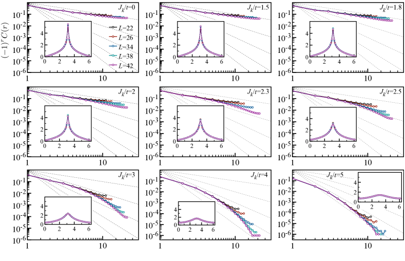
Figure S9: More details of equal time spin correlation shown in Fig. 3 of the main paper. Equal time spin correlation function, $C(r)$, as a function of distance $r$ in log-log scale for various values of $J_{k}/t$ on $4n+2$ lengths chain for $J_{h}//t=1$ and $L_{x}=L_{y}=L=\beta$. The corresponding static spin structure factors $S(k)$ as a function of momentum ($k$) are shown in subfigures. The grey dashed line denotes the $1/r^{n}$ with powers $n$ starting from $n=1$ (first line) to $n=5$ (last line).

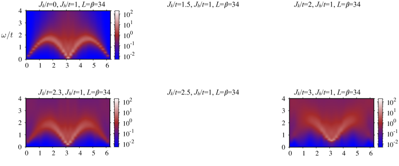
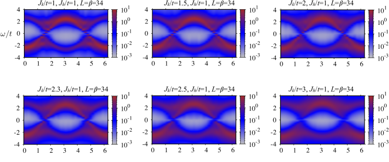
Figure S10: Dynamical spin structure factor, $S(k,\omega)$, as a function of energy ($\omega/t$) and momentum ($k$) along the spin chain for various values of $J_{k}/t$ on $\beta=L=34$ size systems.

Figure S11: Single particle excitations, $A_{0}(k,\omega)$, as a function of energy ($\omega/t$) and momentum ($k$) along Kondo coupled row of conduction electrons for various values of $J_{k}/t$ on $\beta=L=34$ size systems.

References

- Withoff and Fradkin (1990) D. Withoff and E. Fradkin, Phys. Rev. Lett. 64, 1835 (1990).
- Fritz and Vojta (2004) L. Fritz and M. Vojta, Phys. Rev. B 70, 214427 (2004).
- Fritz and Vojta (2013) L. Fritz and M. Vojta, Rep. Prog. Phys. 76, 032501 (2013).
- Vojta (2010) M. Vojta, J. Low Temp. Phys. 161, 203 (2010).
- Yamanaka et al. (1997) M. Yamanaka, M. Oshikawa, and I. Affleck, Phys. Rev. Lett. 79, 1110 (1997).
- Oshikawa (2000) M. Oshikawa, Phys. Rev. Lett. 84, 3370 (2000).
- Senthil et al. (2003) T. Senthil, S. Sachdev, and M. Vojta, Phys. Rev. Lett. 90, 216403 (2003).
- Hofmann et al. (2019) J. S. Hofmann, F. F. Assaad, and T. Grover, Phys. Rev. B 100, 035118 (2019).
- Coleman et al. (2001) P. Coleman, C. Pépin, Q. Si, and R. Ramazashvili, Journal of Physics: Condensed Matter 13, R723 (2001).
- Si et al. (2001) Q. Si, S. Rabello, K. Ingersent, and J. L. Smith, Nature 413, 804 (2001).
- Paschen et al. (2004) S. Paschen, T. Lühmann, S. Wirth, P. Gegenwart, O. Trovarelli, C. Geibel, F. Steglich, P. Coleman, and Q. Si, Nature 432, 881 EP (2004).
- Klein et al. (2008) M. Klein, A. Nuber, F. Reinert, J. Kroha, O. Stockert, and H. v. Löhneysen, Phys. Rev. Lett. 101, 266404 (2008).
- Spinelli et al. (2015) A. Spinelli, M. Gerrits, R. Toskovic, B. Bryant, M. Ternes, and A. F. Otte, Nat. Commun. 6, 10046 (2015).
- Toskovic et al. (2016) R. Toskovic, R. van den Berg, A. Spinelli, I. S. Eliens, B. van den Toorn, B. Bryant, J. S. Caux, and A. F. Otte, Nat. Phys. 12, 656 (2016).
- Choi et al. (2017) D. J. Choi, R. Robles, S. Yan, J. A. J. Burgess, S. Rolf-Pissarczyk, J. P. Gauyacq, N. Lorente, M. Ternes, and L. Sebastian, Nano Lett. 17, 6203 (2017).
- Moro-Lagares et al. (2019) M. Moro-Lagares, R. Korytár, M. Piantek, R. Robles, N. Lorente, J. I. Pascual, M. R. Ibarra, and D. Serrate, Nat. Commun. 10, 2211 (2019).
- Bork et al. (2011) J. Bork, Y.-h. Zhang, L. Diekhöner, L. Borda, P. Simon, J. Kroha, P. Wahl, and K. Kern, Nat. Phys. 7, 901 (2011).
- Zhou et al. (2010) L. Zhou, J. Wiebe, S. Lounis, E. Vedmedenko, F. Meier, S. Blügel, P. H. Dederichs, and R. Wiesendanger, Nat. Phys. 6, 187 (2010).
- Serrate et al. (2010) D. Serrate, P. Ferriani, Y. Yoshida, S.-W. Hla, M. Menzel, K. von Bergmann, S. Heinze, A. Kubetzka, and R. Wiesendanger, Nat Nano 5, 350 (2010).
- Danu et al. (2019) B. Danu, F. F. Assaad, and F. Mila, Phys. Rev. Lett. 123, 176601 (2019).
- Wu et al. (2016) L. Wu, W. Gannon, I. Zaliznyak, A. Tsvelik, M. Brockmann, J.-S. Caux, M. Kim, Y. Qiu, J. Copley, G. Ehlers, et al., Science 352, 1206 (2016).
- Gannon et al. (2019) W. J. Gannon, I. A. Zaliznyak, L. S. Wu, A. E. Feiguin, A. M. Tsvelik, F. Demmel, Y. Qiu, J. R. D. Copley, M. S. Kim, and M. C. Aronson, Nat. Commun. 10, 1 (2019).
- Tsunetsugu et al. (1997) H. Tsunetsugu, M. Sigrist, and K. Ueda, Rev. Mod. Phys. 69, 809 (1997).
- (24) See Supplemental Material, which includes Refs. [Raczkowski and Assaad, 2020; Assaad, 1999; Capponi and Assaad, 2001; Nelder and Mead, 1965], for details of renormalization group analysis, the large-N mean field calculation, and, the details of the QMC results .
- Bercx et al. (2017) M. Bercx, F. Goth, J. S. Hofmann, and F. F. Assaad, SciPost Phys. 3, 013 (2017).
- Blankenbecler et al. (1981) R. Blankenbecler, D. J. Scalapino, and R. L. Sugar, Phys. Rev. D 24, 2278 (1981).
- White et al. (1989) S. R. White, D. J. Scalapino, R. L. Sugar, E. Y. Loh, J. E. Gubernatis, and R. T. Scalettar, Phys. Rev. B 40, 506 (1989).
- Assaad and Evertz (2008) F. F. Assaad and H. G. Evertz, in Computational Many-Particle Physics, Lecture Notes in Physics, Vol. 739, edited by H. Fehske, R. Schneider, and A. Weiße (Springer, Berlin Heidelberg, 2008) pp. 277–356.
- Beach (2004) K. S. D. Beach, arxiv:0403055 (2004).
- Raczkowski and Assaad (2019) M. Raczkowski and F. F. Assaad, Phys. Rev. Lett. 122, 097203 (2019).
- Costi (2000) T. A. Costi, Phys. Rev. Lett. 85, 1504 (2000).
- Luitz et al. (2012) D. J. Luitz, F. F. Assaad, T. Novotný, C. Karrasch, and V. Meden, Phys. Rev. Lett. 108, 227001 (2012).
- Karrasch et al. (2010) C. Karrasch, V. Meden, and K. Schönhammer, Phys. Rev. B 82, 125114 (2010).
- Grover and Senthil (2010) T. Grover and T. Senthil, Phys. Rev. B 81, 205102 (2010).
- Hertz (1976) J. A. Hertz, Phys. Rev. B 14, 1165 (1976).
- Millis (1993) A. J. Millis, Phys. Rev. B 48, 7183 (1993).
- Moriya (2012) T. Moriya, Spin fluctuations in itinerant electron magnetism, Vol. 56 (Springer Science & Business Media, 2012).
- Lobos et al. (2012) A. M. Lobos, M. A. Cazalilla, and P. Chudzinski, Phys. Rev. B 86, 035455 (2012).
- Komijani and Coleman (2019) Y. Komijani and P. Coleman, Phys. Rev. Lett. 122, 217001 (2019).
- Raczkowski and Assaad (2020) M. Raczkowski and F. F. Assaad, Phys. Rev. Research 2, 013276 (2020).
- Assaad (1999) F. F. Assaad, Phys. Rev. Lett. 83, 796 (1999).
- Capponi and Assaad (2001) S. Capponi and F. F. Assaad, Phys. Rev. B 63, 155114 (2001).
- Nelder and Mead (1965) J. A. Nelder and R. Mead, The Computer Journal 7, 308 (1965).
Supplemental Material for: Kondo breakdown in a spin 1/2 chain of adatoms on a Dirac semimetal
Bimla Danu, Matthias Vojta, Fakher F. Assaad and Tarun Grover