Quark-Novae in the outskirts of galaxies: An explanation of the Fast Radio Burst phenomenon

Abstract

We show that old isolated neutron stars in groups and clusters of galaxies experiencing a Quark-Nova phase (QN: an explosive transition to a quark star) may be the source of FRBs. Each of the millions of fragments of the ultra-relativistic QN ejecta provides a collisionless plasma for which the ambient medium (galactic/halo, the intra-group/intra-cluster medium) acts as a relativistic plasma beam. The Buneman and the Weibel instabilities, successively induced by the beam in the fragment, generate particle bunching and observed coherent emission at GHz frequency with a corresponding fluence in the Jy ms range. The duration, frequency drift and the rate are in agreement with observed properties of FRBs. Repeats (on timescales of minutes to months) are due to seeing multiple fragments each beaming at a different direction and coming in at different times. Single (non-repeating) FRBs, occur when only emission from the primary fragment is within the detector’s sensitivity. Key properties of FRB 121102 (its years of activity) and of FRB 180916.J0158$+$65 (its $\sim 16$ day period) are recovered. The spatial and temporal coincidence between SGR 1935$+$2154 and FRB 200428 finds an explanation in our model. We give testable predictions.

1 Introduction

FRB science began with the Lorimer burst (Lorimer et al. 2007) and followed with a decade of discovery of dozens of intense, millisecond, highly dispersed radio bursts in the GHz range (see http://frbcat.org/; Petroff et al. 2016). An FRB may consist of single or multiple pulses of milliseconds duration. While most FRBs were one-off events, a few were repeats (Spitler et al. 2016; Scholz et al. 2016; CHIME/FRB Collaboration 2019a, b). FRB dispersion measures (DM) of hundreds of pc cm^-3 put them at extra-Galactic to cosmological distances which makes them very bright ($>10^{41}$ erg s^-1) with their high brightness temperatures requiring a coherent emission mechanism (Kellermann & Pauliny-Toth 1969; see also Katz 2014; Popov et al. 2018).

Observations and derived properties of FRBs can be found in the literature (Thornton et al. 2013; Spitler et al. 2014; Kulkarni et al. 2014; Petroff et al. 2016; Ravi et al. 2016; Gajjar et al. 2018; Michilli et al. 2018; Lorimer 2018; Cordes & Chatterjee 2019). The large beams of current radio telescopes makes it difficult to pin-point the host galaxies of most FRBs let alone their association with known astrophysical objects. This makes it hard to constrain models despite the numerous ideas suggested (Platts et al. 2018). The X-ray activity of the galactic soft $\gamma$-ray repeater (SGR) 1935$+$2154 (Barthelmy et al. 2020) coincided spatially with FRB 200428 (Scholz et al. 2020; CHIME/FRB Collaboration 2020; Witze 2020; Bochenek et al. 2020). This supports the association of at least some FRBs with SGRs. The repeating nature of FRBs has been used to argue against catastrophic scenarios, but we show that is not necessarily the case.

In the QN model, a massive NS ($\sim 2M_{\odot}$; born from stellar progenitors in the 20-40$M_{\odot}$ mass range) converts spontaneously to a quark star (QS) when quark deconfinement in its core, and the subsequent explosive combustion of neutrons to quarks, is triggered either by: (i) spin-down if born rapidly rotating with a period of a few milliseconds (Staff et al. 2006); (ii) quark nucleation on timescales of hundreds of millions of years if born slowly rotating. During the QN, the outermost layers of the NS are ejected at ultra-relativistic speeds. From Ouyed & Leahy (2009), the QN ejecta breaks up into millions of dense fragments in a plasma state (hereafter “chunks"). In case (i), the QN occurs within years of a core-collapse SN (ccSN) explosion of a massive star with the chunks embedded in the SN. In case (ii) the QN occurs in the outskirts of galaxies. Ouyed al. (2020) showed that the interaction of the chunks with the expanded SN ejecta gives properties (intermittency, light-curve and spectrum) of long-duration Gamma-ray bursts (LGRBs). Here, we focus on isolated QNe; old NSs experiencing the QN phase, outside their birth galaxies.

Slowly rotating, massive NSs rely on quark nucleation in their core to trigger the QN. For nucleation timescales $\geq 10^{8}$ years (e.g. Bombaci et al. 2004; Harko et al. 2004), a candidate NS with a typical kick velocity of $\sim 300$ km s^-1 travels a distance $>\sim 30$ kpc from its birth place. It would explode in the intra-group or intra-cluster medium. The chunks travel through the ambient medium/plasma and expand until they become collisionless. They experience two inter-penetrating collisionless instabilities: the Buneman instability (BI) then the Buneman-induced thermal Weibel instability (WI). This triggers particle bunching, coherent synchrotron emission (CSE) and FRBs as shown here. The fragmented nature of the QN ejecta (with every chunk emitting in a specific direction and at a different time) allows repetition. Thus FRBs from a QN, a one-off cataclysmic event, are inherently repeaters with single (non-repeating) FRBs, occurring when only emission from the primary chunk is detected.

Hereafter, unprimed quantities are in the chunk’s reference frame while the superscripts “ns" and “obs." refer to the NS frame (i.e. the ambient medium) and the observer’s frame, respectively. The transformation from the local NS frame to the chunk’s frame is $dt^{\rm ns}=\Gamma_{\rm c}dt$ while the transformations from the chunk’s frame to the observer’s frame are $dt^{\rm obs.}=(1+z)dt/D(\Gamma_{\rm c},\theta_{\rm c})$, $\nu^{\rm obs.}=D(\Gamma_{\rm c},\theta_{\rm c})\nu/(1+z)$ with $z$ the source’s redshift and $\theta_{\rm c}$ the angle between the observer and chunk’s velocity vectors; $D(\Gamma_{\rm c},\theta_{\rm c})$ is the chunk’s Doppler factor with $\Gamma_{\rm c}$ the Lorentz factor.

We consider three media: (i) the intra-group medium (IGpM), with number density $n_{\rm amb.}^{\rm ns}\simeq 10^{-4}$-$10^{-2}$ cm^-3 (e.g. Cavaliere 2000); (ii) the intra-galaxy cluster medium (ICM) with $n_{\rm amb.}^{\rm ns}\simeq 10^{-4}$-$10^{-2}$ cm^-3 (e.g. Fabian 1994); (iii) the intergalactic medium (IGM) with $n_{\rm amb.}^{\rm ns}\simeq 10^{-7}$ cm^-3 (e.g. McQuinn 2016). Hereafter ICM refers jointly to the hot diffuse gas observed in groups and clusters of galaxies. Because the majority of galaxies are in groups (e.g. Tully 1987) we take conditions in the IgCM with ambient density of $n_{\rm amb.}^{\rm ns}=10^{-3}$ cm^-3 as our fiducial value. The paper focuses on the interaction of the QN chunks with such an ambient medium and is structured as follows: In §2 we give an overview of the QN ejecta, and how it becomes collisionless as it travels in the ambient medium. We describe the relevant plasma instabilities (BI and WI) and the resulting CSE. The application to FRBs is done in §3. In §4, we list our model’s predictions and limitations, and conclude in §5.

2 The QN and its ejecta

The energy release during the conversion of a NS to a QS is $\sim 3.8\times 10^{53}\ {\rm erg}\times(M_{\rm NS}/2M_{\odot})\times(\Delta E_{\rm dec.}/100\ {\rm MeV})$ for a NS mass of $M_{\rm NS}=2M_{\odot}$ and a conversion energy release of $\Delta E_{\rm dec.}=100$ MeV per neutron (Weber (2005)). This is a fraction of the combined conversion energy and gravitational binding energy (Keränen et al. 2005; Niebergal 2011; Ouyed, A 2018; Ouyed al. 2020). A large part is in kinetic energy of the QN ejecta $E_{\rm QN}\sim 10^{52}$-$10^{53}$ erg when the converting NS is hot (as in the case of a QN in the wake of a ccSN (Ouyed al. (2020)). For the case of an old isolated cold NS, the very slow nucleation timescales means that most of the conversion energy is lost to neutrinos yielding a kinetic energy $E_{\rm QN}\sim 10^{51}$-$10^{52}$ erg. The QN ejecta consists of the outermost crust layers of the NS with a mass $M_{\rm QN}\sim 10^{-5}M_{\odot}$ and a Lorentz factor $\Gamma_{\rm QN}=E_{\rm QN}/(M_{\rm QN}c^{2})\simeq 10^{2}$-$10^{3}$.

2.1 Ejecta properties and statistics

With $N_{\rm c}=10^{6}$ the number of chunks, a typical mass is $m_{\rm c}=M_{\rm QN}/N_{\rm c}\simeq 10^{22.3}\ {\rm gm}\times M_{\rm QN,28.3}/N_{\rm c,6}$. The chunk’s Lorentz factor is taken to be constant with $\Gamma_{\rm c}=\Gamma_{\rm QN}=10^{2.5}$ for a QN ejecta’s kinetic energy $E_{\rm QN}=\Gamma_{\rm c}M_{\rm QN}c^{2}\simeq 5.7\times 10^{51}$ erg; i.e. 1% of the conversion energy is converted to kinetic energy; these values are listed in Table 4.

In Appendix SA we summarize chunk properties:

• The chunks are equally spaced in solid angle $\Omega$ around the explosion site. Defining $N_{\theta_{\rm c}}$ as the number of chunks per angle $\theta_{\rm c}$, we write $dN_{\theta_{\rm c}}/d\Omega=const.=N_{\rm c}/4\pi$ with $d\Omega=2\pi\sin{\theta_{\rm c}}d\theta_{\rm c}$ so that $dN_{\theta_{\rm c}}/d\theta_{\rm c}=(N_{\rm c}/2)\sin{\theta_{\rm c}}\simeq(N_{\rm c}/2)\theta_{\rm c}$ with $\theta_{\rm c}<<1$. Because $N_{\rm c}\pi\Delta\theta_{\rm c}^{2}=4\pi$, the average angular separation is

  $$\Delta\theta_{\rm s}=2\Delta\theta_{\rm c}=\frac{4}{N_{\rm c}^{1/2}}\simeq\frac{4\times 10^{-3}}{N_{\rm c,6}^{1/2}}\ ,$$ (1)

  yielding $\Delta\theta_{\rm s}\sim 1/\Gamma_{\rm c}$ for $N_{\rm c}=10^{6}$ and $\Gamma_{\rm c}=10^{2.5}$.

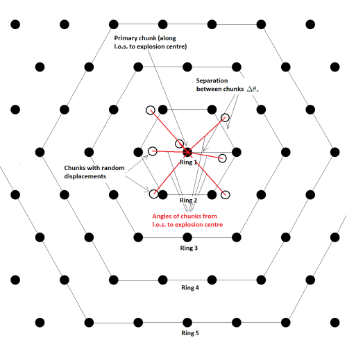
Figure 4: Honeycomb geometry: Illustration of observer’s face on view of distribution of chunks. Uniformly spaced case: The solid black circles represent evenly spaced chunks travelling radially outward from the QN site with the primary chunk (labelled “ring" 1) travelling at angle $0^{\circ}$ with respect to the line-of-sight (l.o.s) to the QN. The 6 chunks in “ring" 2 all travel at angle $\Delta\theta_{s}$ (see Eq. (15)) from the l.o.s.. The 12 chunks in “ring" 3 all travel at angle $2\Delta\theta_{s}$ from the l.o.s, and so on for successively outward rings. The time delays of received FRB emission by the observer are determined by the angular time delays which depends on angle from the l.o.s.. Thus the FRB emission from the chunks in “ring" 2 all arrive at the same time. Randomly spaced case: The open circles represent randomly spaced chunks (only illustrated for “ring" 1 and “ring" 2), which are offset at small random angles and directions from the uniformly spaced case. In this case the arrival times of the different chunks in a given ring (e.g. “ring" 2) are different, again depending on the l.o.s. angle of each chunk.

  The geometry for chunk angular spacing is a 2-dimensional honeycomb (see Figure 4) with 1 primary ($i=1$) chunk at $0\leq\theta_{\rm c}<\Delta\theta_{\rm c}$ and $6\times(i-1)$ chunks for subsequent, and concentric, “rings" (with $i\geq 2$; 6 secondary chunks, 12 tertiary chunks etc..). The mean angle of the primary (P), secondary (S) and tertiary (T) chunks are $\bar{\theta}_{\rm P}\simeq 4/(3N_{\rm c,6}^{1/2})$, $\bar{\theta}_{\rm S}\simeq 2.3\bar{\theta}_{\rm P}$ and $\bar{\theta}_{\rm T}\sim 6\bar{\theta}_{\rm P}$ (Eq. (• ‣ SA));

• with $\Gamma_{\rm c}^{2}>>1$ and $\theta_{\rm c}<<1$, the Doppler factor is $D_{\rm c}(\Gamma_{\rm c},\theta_{\rm c})\simeq 2\Gamma_{\rm c}/f(\theta_{\rm c})$ with

  $$f(\theta_{\rm c})=1+(\Gamma_{\rm c}\theta_{\rm c})^{2}\ ,$$ (2)

  and $f(\theta_{\rm c})<<\Gamma_{\rm c}^{2}$. The average values are

  $$f(\bar{\theta}_{\rm P})\sim 1+0.18\frac{\Gamma_{\rm c,2.5}^{2}}{N_{\rm c,6}}$$

  $$f(\bar{\theta}_{\rm S})\sim 1+0.97\frac{\Gamma_{\rm c,2.5}^{2}}{N_{\rm c,6}}$$

  $$f(\bar{\theta}_{\rm T})\sim 1+6.67\frac{\Gamma_{\rm c,2.5}^{2}}{N_{\rm c,6}}\ ;$$ (3)

• The average change in $f(\theta_{\rm c})$ from one chunk to another with respect to the observer is (see Eq. (21)):

  $$\Delta f^{\rm chunks}\simeq\frac{1.6}{\pi}\times\frac{\Gamma_{\rm c,2.5}^{2}}{N_{\rm c,6}}\ .$$ (4)

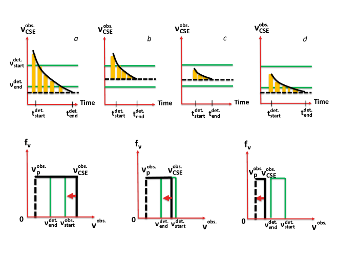
Figure 1: Top panels: Schematic representation of frequency drifting in time (Eq. (3)) for a flat emitted spectrum. The detector has maximum and minimum frequencies $\nu_{\rm max.}^{\rm det.}$ and $\nu_{\rm min.}^{\rm det.}$. The possible scenarios are: a) $\nu_{\rm CSE,max.}^{\rm obs.}(\theta_{\rm c})>\nu_{\rm max.}^{\rm det.}$ and $\nu_{\rm p,e}^{\rm obs.}(\theta_{\rm c})<\nu_{\rm min.}^{\rm det.}$; b) $\nu_{\rm CSE,max.}^{\rm obs.}(\theta_{\rm c})>\nu_{\rm max.}^{\rm det.}$ and $\nu_{\rm min.}^{\rm det.}<\nu_{\rm p,e}^{\rm obs.}(\theta_{\rm c})<\nu_{\rm max.}^{\rm det.}$; c) $\nu_{\rm max.}^{\rm det.}>\nu_{\rm CSE,max.}^{\rm obs.}(\theta_{\rm c})$ and $\nu_{\rm p,e}^{\rm obs.}(\theta_{\rm c})>\nu_{\rm min.}^{\rm det.}$; d) $\nu_{\rm max.}^{\rm det.}>\nu_{\rm CSE,max.}^{\rm obs.}(\theta_{\rm c})>\nu_{\rm min.}^{\rm det.}$ and $\nu_{\rm p,e}^{\rm obs.}(\theta_{\rm c})<\nu_{\rm min.}^{\rm det.}$. The vertical bands indicate the range of detected frequencies at any given time. The horizontal dashed line is the chunk’s plasma frequency $\nu_{\rm p,e}^{\rm obs.}(\theta_{\rm c})$. Bottom panels: The spectrum at three different times for case “a". The arrow shows the frequency decreasing in time and drifting through the detector’s band.

2.2 The collisionless QN chunks

The evolution of the QN chunks is given in Ouyed & Leahy (2009). The later evolution is:

(i) The QN chunk becomes optically thin to photons when it expands to a radius $R_{\rm c,opt.}\simeq 2.2\times 10^{10}\ {\rm cm}\times m_{\rm c,22.3}^{1/2}\kappa_{\rm c,-1}^{1/2}$, using $R_{\rm c}=1/\kappa_{\rm c}\rho_{\rm c}$; $\kappa_{\rm c}=0.1$ cm² gm^-1 is the opacity, $\rho_{\rm c}=n_{\rm c}m_{\rm H}=(3m_{\rm c}/4\pi R_{\rm c}^{3})\times m_{\rm H}$ is its density and $m_{\rm H}$ the hydrogen mass. The baryon number density is $n_{\rm c,opt.}=3m_{\rm c}/4\pi R_{\rm c,opt.}^{3}m_{\rm H}\simeq 2.8\times 10^{14}\ {\rm cm}^{-3}\times m_{\rm c,22.3}^{-1/2}\kappa_{\rm c,-1}^{-3/2}$;

(ii) The chunk is optically thin to hadronic collisions when it expands to a radius $R_{\rm c,HH}\simeq 1.5\times 10^{9}\ {\rm cm}\times m_{\rm c,22.3}^{1/2}\sigma_{\rm HH,-27}^{1/2}$, from $R_{\rm c}=1/n_{\rm c}\sigma_{\rm HH}$; $\sigma_{\rm HH,-27}$ is the hadron-hadron cross-section in milli-barns (Letaw et al. 1983);

(iii) A chunk is subject to electron Coulomb collisions so it thermalizes and expands beyond $R_{\rm c,opt.}$ from internal pressure. The electron Coulomb collision length for number density $n_{\rm c}$ and temperature $T_{\rm c}$ is (Richardson 2019) $\lambda_{\rm c,C}\simeq 1.1\times 10^{4}\ {\rm cm}\times T_{\rm c}^{2}/n_{\rm c}$ with Coulomb parameter $\ln{\Lambda}=20$ (Lang 1999). During the early evolution $\lambda_{\rm c,C}<<R_{\rm c}$.

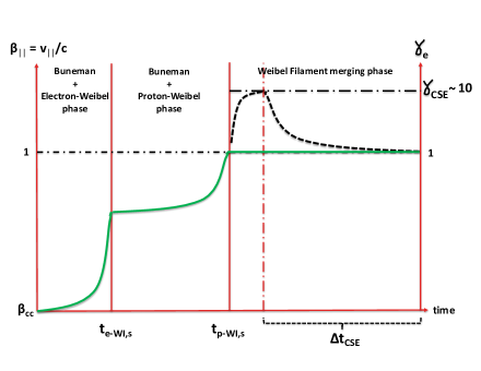
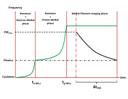
Figure 5: Top panel: A schematic representation of the evolution of $\beta_{\parallel}=v_{\parallel}/c$ during the BI-WI phases; $\beta_{\perp}=0.1\beta_{\parallel}$ (not shown here). In the linear phase for $t<t_{\rm p-WI,s}$ (i.e. up to the saturation of the proton-Weibel phase; see Appendix SC), the BI heating of chunk electrons (i.e. the increase in $\beta_{\parallel}$) is converted by WI into magnetic field amplification, into magnetic turbulence and into currents. In this regime, $\beta_{\parallel}$ increases from $\beta_{\parallel}\sim\beta_{\rm cc}$ (where $v_{\rm cc}$ is the electron thermal speed when the chunk become collisionless; see Eq. (32)) to $\beta_{\parallel}\sim 1$. During filament merging, magnetic turbulence and current dissipation accelerates electrons to relativistic speed, $\gamma_{\rm CSE}>>1$, shutting-off the BI. The BI requires the drift velocity (here the light speed $c$) between the beam protons and the chunk’s electrons to exceed the thermal speed of the chunk’s electrons (see Appendix SC). The decrease in $\gamma_{\rm CSE}$ is due to Coherent Synchrotron Emission (CSE) cooling. Lower panel: A schematic representation of the evolution of the different frequencies during the BI-WI process in our model. The electron plasma frequency ($\nu_{\rm p,e}=\sqrt{4\pi n_{\rm cc}e^{2}/m_{\rm e}}$, dot-dashed horizontal line) remains constant. The electron cyclotron frequency ($\nu_{\rm B}=eB_{\rm c}/m_{\rm e}c$, thick green line) saturates first during the e-WI phase when $\nu_{\rm B}\sim\nu_{\rm p,e}$ (i.e. $B_{\rm c}=B_{\rm e-WI,s}$) and later at the end of the p-WI phase with $\nu_{\rm B}\sim\sqrt{m_{\rm p}/m_{\rm e}}\nu_{\rm p,e}$ (i.e. $B_{\rm c}=B_{\rm p-WI,s}$). CSE at frequency $\nu_{\rm CSE}$ is triggered throughout the filament merging phase when $\nu_{\rm CSE}<<\gamma_{\rm CSE}^{2}\sqrt{m_{\rm p}/m_{\rm e}}\nu_{\rm p,e}$ is satisfied (see Appendix SD). The CSE frequency $\nu_{\rm CSE}$ decreases over time (the thick black line) due to the increase in bunch size during filament merging. CSE ceases when its frequency drops to the chunk’s plasma frequency ($\nu_{\rm p,e}$). The end of filament merging occurs when the filaments grow to a size of the order of the beam’s protons Larmor radius. The trapping of the protons is followed by the formation of the Weibel shock (not shown here), quickly decelerating the chunk and putting an end to the BI-WI process.

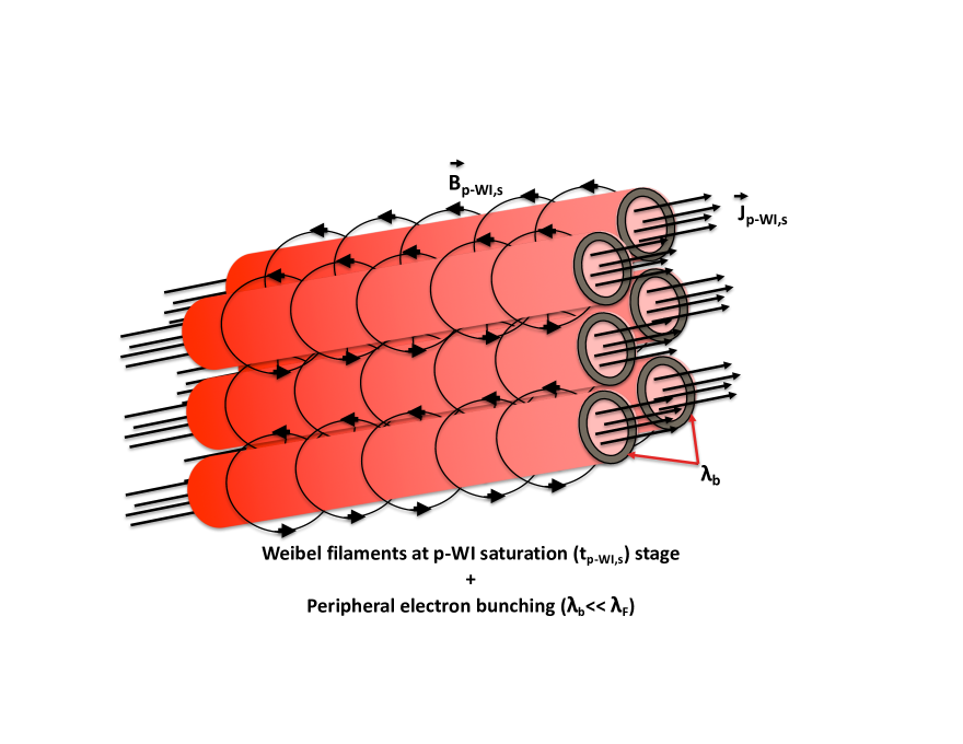
Figure 6: A schematic representation of Weibel filament and electron bunch geometry: Bunches are shown as cylindrical shells with thickness $\lambda_{\rm b}$ (shown by the dark-grey shadding) around the Weibel cylindrical filaments of diameter $\lambda_{\rm F}$ ($\lambda_{\rm b}<<\lambda_{\rm F}$). The bunches, tied to the Weibel filaments, extend across the QN chunk (the background plasma) in the direction parallel to the beam’s direction (here the ICM). Also illustrated are the Weibel saturated magnetic field, $\vec{B}_{\rm p-WI,s}$ (see Appendix SC and Eq. (2)) reached at the end of the proton-Weibel (p-WI) phase, and the corresponding filament currents, $\vec{J}_{\rm p-WI,s}$.

After the chunk is optically thin, hadronic collisions continue to heat it. From Appendix SB, hadronic collisions with the ambient medium and thermalization from Coulomb collisions expand the chunk until it becomes collisionless when $R_{\rm c}=\lambda_{\rm c,C}$. Table 5 lists the number density ($n_{\rm cc}$), radius ($R_{\rm cc}$) and thermal speed ($\beta_{\rm cc}=v_{\rm cc}/c$) of a typical chunk when it becomes collisionless. At this stage, its interaction with the ICM triggers the BI and WI (Appendix SC and Figure 5), yielding particle bunching and CSE (Appendix SD and Figure 6) with observed properties (frequency, duration and fluence) similar to FRBs.

Chunk electrons bunch up on scales $\lambda_{\rm b}(t)$ yielding CSE at a frequency $\nu_{\rm CSE}(t)=c/\lambda_{\rm b}(t)$. It decreases in time, due to bunches merging and increasing in size, as (Eq. (3)) $\nu_{\rm CSE}(t)=\nu_{\rm CSE}(0)\times(1+t/t_{\rm m-WI})^{-\delta_{\rm m-WI}}$ with $t_{\rm m-WI}$ the characteristic merging timescale (Eq. (SC.3)). CSE ceases when $\nu_{\rm CSE}(t)$ drops to the chunk’s plasma frequency, $\nu_{\rm p,e}\simeq 9\ {\rm kHz}\times n_{\rm cc}^{1/2}$ (Lang 1999), and can no longer escape. In the observer’s frame, the initial (maximum) CSE frequency is $\nu_{\rm CSE,max.}^{\rm obs.}(\theta_{\rm c})=D(\Gamma_{\rm c},\theta_{\rm c})\nu_{\rm CSE}(0)/(1+z)$, its duration is $\Delta t_{\rm CSE}^{\rm obs.}=(1+z)\Delta t_{\rm CSE}/D(\Gamma_{\rm c},\theta_{\rm c})$, and the luminosity is $L_{\rm CSE}^{\rm obs.}(\theta_{\rm c})=(D(\Gamma_{\rm c},\theta_{\rm c})^{4}/(1+z)^{2})L_{\rm CSE}$; $\nu_{\rm CSE}(0),L_{\rm CSE}(0)$ and $\Delta t_{\rm CSE}$ are derived in Appendix SD. I.e.

$$\nu_{\rm CSE,max.}^{\rm obs.}(\theta_{\rm c}) \simeq\frac{11.6\ {\rm GHz}}{(1+z)f(\theta_{\rm c})}\times\delta_{\rm CSE,-1}\gamma_{\rm CSE,1}^{2}\times\Gamma_{\rm c,2.5}n_{\rm cc,1}^{1/2}$$ (5)

$$L_{\rm CSE}^{\rm obs.}(\theta_{\rm c}) \simeq\frac{4.7\times 10^{46}\ {\rm erg\ s}^{-1}}{(1+z)^{2}f(\theta_{\rm c})^{4}}\times\frac{\zeta_{\rm BI,-1}\beta_{\rm WI,-1}}{\zeta_{\rm m-WI,2}}\times$$

$$\times\frac{\Gamma_{\rm c,2.5}^{6}R_{\rm cc,15}^{2}n_{\rm amb.,-3}^{\rm ns}}{\beta_{\rm cc,-2}}$$ (6)

$$\Delta t_{\rm CSE}^{\rm obs.}(\theta_{\rm c}) \simeq\left(\left(642.7\delta_{\rm CSE,-1}\gamma_{\rm CSE,1}^{2}\right)^{\frac{1}{\delta_{\rm m-WI}}}-1\right)\times t_{\rm m-WI}^{\rm obs.}(\theta_{\rm c})\ ,$$ (7)

with the observed characteristic bunch merging timescale:

$$t_{\rm m-WI}^{\rm obs.}(\theta_{\rm c})=\frac{(1+z)}{D(\Gamma_{\rm c},\theta_{\rm c})}t_{\rm m-WI}\simeq 0.24\ {\rm ms}\times(1+z)f(\theta_{\rm c})\times\frac{\zeta_{\rm m-WI,2}}{\Gamma_{\rm c,2.5}n_{\rm cc,1}^{1/2}}\ .$$ (8)

The parameters $\delta_{\rm CSE},\gamma_{\rm CSE},\zeta_{\rm BI},\beta_{\rm WI},\zeta_{\rm m-WI},\delta_{\rm m-WI}$ are defined and given in Table 4.

The observed CSE frequency decreases in time as (Eq. (3)) $\nu_{\rm CSE}^{\rm obs.}(\theta_{\rm c},t^{\rm obs.})=\nu_{\rm CSE,max.}^{\rm obs.}(\theta_{\rm c})\times(1+t^{\rm obs.}/t_{\rm m-WI}^{\rm obs.}(\theta_{\rm c}))^{-\delta_{\rm m-WI}}$ reaching a minimum value of

$$\nu_{\rm CSE,min}^{\rm obs.}(\theta_{\rm c})=\frac{D(\Gamma_{\rm c},\theta_{\rm c})}{1+z}\nu_{\rm p,e}\simeq\frac{18\ {\rm MHz}}{(1+z)f(\theta_{\rm c})}\times\Gamma_{\rm c,2.5}n_{\rm cc,1}^{1/2}\ .$$ (9)

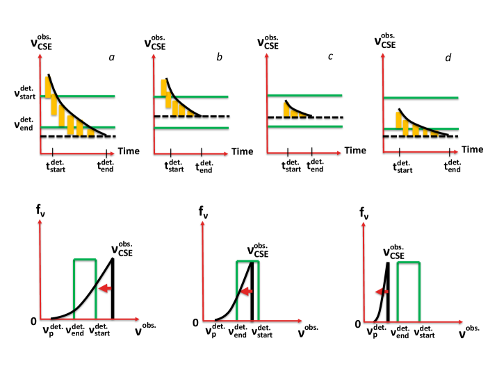
Figure 7: Same as in Figure 1 in the main paper but here for the case of a power-law spectrum with positive index $\alpha_{\rm CSE}$. The difference is that for a steep spectrum only the emission near the peak frequency (the narrower vertical bands) is detected at a given time.

Figure 1 illustrates frequency drifting in time through the detector’s band for the case of a flat spectrum. The vertical bands indicate that CSE emerges from the chunk at frequencies $\nu_{\rm CSE,min.}^{\rm obs.}(\theta_{\rm c})\leq\nu_{\rm CSE}^{\rm obs.}(\theta_{\rm c},t^{\rm obs.})\leq\nu_{\rm CSE,max.}^{\rm obs.}(\theta_{\rm c})$. For the steep power-law spectrum case (Figure 7), CSE is detectable around the peak frequency. The frequency bands at a given time are narrower in the case of the steep power-law spectrum case, more like observed FRBs.

Table 1: Selected FRB detectors

Telescope	Band (MHz)	sensitivity (Jy ms)
Arecibo1	$\sim$ 1210-1530	$\sim 0.1$
Parkes2	$\sim$ 1180-1580	$\sim 1$
ASKAP3	$\sim$ 1210-1530	$\sim$ 10
CHIME4	$\sim$ 400-800	$\sim 0.1$
LOFAR5	$\sim$ 110-240	$>10^{3}$

¹http://www.naic.edu/alfa/gen_info/info_obs.shtml.
²https://www.parkes.atnf.csiro.au/cgi-bin/public_wiki/wiki.pl?MB20.
³https://www.atnf.csiro.au/projects/askap/index.html.
⁴https://chime-experiment.ca/instrument.
⁵ LOFAR’s high-band antenna (van Haarlem et al. 2013).

Table 2: Simulations: a repeating FRB (yielding the waterfall plot in Figure 3) from an ICM-QN at $z=0.2$ with $N_{\rm c}=10^{5},\log{\Gamma_{\rm c}}=2.5,\log{m_{\rm c}}\ {\rm(gm)}=22.55$; other parameters are the fiducial values listed in Table 4. The QN FRB simulator can be run at: http://www.quarknova.ca/FRBSimulator/.

Detections ($\theta_{\rm c}(\#0)=5.47$E-3)¹

#	$\Delta\theta_{\rm c}$ (rad)2	$f(\theta_{\rm c})$	$t_{\rm OA}^{\rm obs.}$ (days)	$\Delta t_{\rm OA}^{\rm obs.}$ (days)3	Frequency (MHz)4	Width (ms)	Fluence (Jy ms)5
0	0.00	3.99	0.00	0.00	3.00E3	0.93	CHIME (64.00)
							Parkes (5.56)
							Arecibo (4.6)
1	2.05E-3	6.65	9.23	9.23	1.80E3	1.55	CHIME (8.27)
							Arecibo (0.6)
2	1.84E-3	9.76	19.99	10.76	1.23E3	2.27	CHIME (1.79)
3	7.71E-4	11.26	25.20	5.20	1.06E3	2.62	CHIME (1.01)

Here, and in all tables in the online supplementary material (SM):
¹ $\theta_{\rm c}(\#0)$ is the viewing angle in radians of the first detected chunk.
² $\Delta\theta_{\rm c}$ is the difference between the current chunk’s $\theta_{\rm c}$ and the previous one that arrived.
³ $\Delta t_{\rm OA}^{\rm obs.}$ is the time-delay (difference in time-of-arrival, $t_{\rm OA}^{\rm obs.}$) between successive bursts.
⁴ Shown is the maximum CSE frequency $\nu_{\rm CSE}^{\rm obs.}(\theta_{\rm c})$ (Eq. (7)).
⁵ Only detectors with fluence above sensitivity threshold (see Table 1) are shown.

3 FRBs from ICM-QNe

Listed in Table 5 are frequency, duration and fluence of the resulting FRBs. For a detector with bandwidth $\Delta\nu^{\rm det.}=\nu_{\rm max.}^{\rm det.}-\nu_{\rm min.}^{\rm det.}$ ($\nu_{\rm max.}^{\rm det.}$ and $\nu_{\rm min.}^{\rm det.}$ are the maximum and minimum frequency):

(i) If $\nu_{\rm CSE,max.}^{\rm obs.}(\theta_{\rm c})>\nu_{\rm max.}^{\rm det.}$ and $\nu_{\rm CSE,min.}^{\rm obs.}(\theta_{\rm c})<\nu_{\rm min.}^{\rm det.}$, the duration of the CSE is set by the time it takes emission to drift through the detector’s band (Eq. (SE.2)):

$$\Delta t_{\rm CSE}^{\rm det.}(\theta_{\rm c}) =t_{\rm m-WI}^{\rm obs.}(\theta_{\rm c})\times$$

$$\times\left(\left(\frac{\nu_{\rm CSE,max.}^{\rm obs.}(\theta_{\rm c})}{\nu_{\rm min.}^{\rm det.}}\right)^{1/\delta_{\rm m-WI}}-\left(\frac{\nu_{\rm CSE,max.}^{\rm obs.}(\theta_{\rm c})}{\nu_{\rm max.}^{\rm det.}}\right)^{1/\delta_{\rm m-WI}}\right)\ .$$ (10)

The FRB duration is the minimum between the CSE duration and the drifting time through the detector’s band

$$\Delta t_{\rm FRB}^{\rm obs.}(\theta_{\rm c})={\rm MIN}\left[\Delta t_{\rm CSE}^{\rm obs.}(\theta_{\rm c}),\Delta t_{\rm CSE}^{\rm det.}(\theta_{\rm c})\right]\ ;$$ (11)

(ii) The band-integrated fluence for a flat spectrum is $F(\theta_{\rm c},\delta_{\rm m-WI},0)=\mathcal{F}(\theta_{\rm c},0)\times\mathcal{G}(\theta_{\rm c},\delta_{\rm m-WI},0)$ with $\mathcal{F}(\theta_{\rm c},0)$ given by Eq. (28) as

$$\mathcal{F}(\theta_{\rm c},0) \simeq 810\ {\rm Jy\ ms}\ \frac{1}{f(\theta_{\rm c})^{2}d_{\rm L,27.5}^{2}}\times\frac{\zeta_{\rm BI,-1}\beta_{\rm WI,-1}}{\delta_{\rm CSE,-1}\gamma_{\rm CSE,1}^{2}}\times$$

$$\times\frac{\Gamma_{\rm c,2.5}^{4}R_{\rm cc,15}^{2}{n_{\rm amb.,-3}^{\rm ns}}}{n_{\rm cc,1}\beta_{\rm cc,-2}}\ ,$$ (12)

with $\mathcal{G}(\theta_{\rm c},\delta_{\rm m-WI},0)$ (Eq. (27)) varying from a few to a few thousands depending on the detector’s band (Table 6); the luminosity distance is $d_{\rm L}\simeq 1$ Gpc for sources at $z=0.2$.

Also listed in Table 5 is the timescale between repeats $\Delta t_{\rm repeat}^{\rm obs.}$ (emission from two separate chunks) found by setting $f(\theta_{\rm c})=(1.6/\pi)\times\Gamma_{\rm c,2.5}^{2}/N_{\rm c,6}$ (Eq. (4)) in $t_{\rm cc}^{\rm obs.}$ (Eq. (34)):

$$\Delta t_{\rm repeat}^{\rm obs.}\simeq 1.3\ {\rm days}\times(1+z)\times\frac{1}{N_{\rm c,6}}\times\left(\frac{m_{\rm c,22.3}\kappa_{\rm c,-1}}{\sigma_{\rm HH,-27}^{3}\Gamma_{\rm c,2.5}({n_{\rm amb.,-3}^{\rm ns}})^{3}}\right)^{1/5}\ .$$ (13)

The delay between two successive CSE bursts (two different emitting chunks) for an ICM-QN depends mainly on $N_{\rm c}$. For fiducial parameter values, typical time between repeats is of the order of days in the observer’s frame.

Table 7 shows examples of FRBs from ICM-QNe obtained using the equations in Table 5. Because $f(\bar{\theta}_{\rm c})=1+(\Gamma_{\rm c}\bar{\theta}_{\rm c})^{2}$ (Eq. (17)) is controlled by $N_{\rm c}$ ($\theta_{\rm c}\propto 1/N_{\rm c}^{1/2}$) and $\Gamma_{\rm c}$, we vary these parameters and show a range in viewing angles on FRB detections in our model. Chunks with $\nu_{\rm CSE,max.}^{\rm obs.}(\theta_{\rm c})>\nu_{\rm max.}^{\rm det.}$ will eventually be detected when the frequency drifts into the detector’s band. The drift ends when the CSE frequency reaches $\mathbf{{\rm MAX}}(\nu_{\rm min.}^{\rm det.},\nu_{\rm CSE,min.}^{\rm obs.}(\theta_{\rm c}))$. For fiducial parameters values, the plasma frequency $\nu_{\rm p,e}^{\rm obs.}(\theta_{\rm c})$ is below the detector’s minimum frequency which implies that CSE drifts through the band (Figure 1). The fluences per detector are given in Table 7 with the shaded cells showing the values within detector’s sensitivity (Table 1). Repetition (see Appendix SE.6) is set by the angular separation between emitting chunks which yields a roughly constant time delay between bursts. Boxes A, B and C in Table 7, show that typical time delays between bursts within a repeating FRB is $12\ {\rm days}<\Delta t_{\rm repeat}^{\rm obs.}<20\ {\rm days}$.

3.1 Simulations

A parameter survey was performed by simulating the QN chunks starting from the moment when they become a collisionless plasma within the ICM: (i) We distribute the chunks on the surface of a unit sphere using the “Regular Placement" algorithm (Deserno 2004). The chunks are placed along rings of constant latitude, and evenly spaced over the sphere. The simulation then chooses a random direction vector from which to view the sphere, and calculates the $\theta_{\rm c}$ angle of each chunk based on this vector; (ii) The zero time of arrival $t_{\rm OA}^{\rm obs.}=0$ is set by the chunk which has the minimum value of $t_{\rm cc}^{\rm obs.}$. The time of arrival of subsequent chunks, $t_{\rm OA}^{\rm obs.}(\theta_{\rm c})$, are recorded with respect to the signal from the first detected chunk. The time delay between successive chunks we define as $\Delta t_{\rm OA}^{\rm obs.}$ and $\Delta\theta_{\rm C}$ as the difference between the current chunk’s $\theta_{\rm c}$ and the previous one that arrived; (iii) We take $E_{\rm QN}=10^{51}$ erg which fixes the chunk’s mass for a given $N_{\rm c}$ and $\Gamma_{\rm c}$; $m_{\rm c}=E_{\rm QN}/N_{\rm c}\Gamma_{\rm c}c^{2}$; (iv) For non-constant chunk mass simulations, we sample the mass from a Gaussian distribution with a mean $\bar{m}_{\rm c}=E_{\rm QN}/N_{\rm c}\Gamma_{\rm c}c^{2}$ and standard deviation $\sigma_{\rm\log(m_{\rm c})}=1.0$.

Single FRBs are detector-dependent and occur when one of the conditions in Eq. (29) is violated, which occurs mostly when $f(\bar{\theta}_{\rm T})>>f(\bar{\theta}_{\rm S})>>f(\bar{\theta}_{\rm P})>>1$ (Appendix SE.6). This is the case when considering fewer QN chunks (typically $N_{\rm c}=10^{5}$) and higher Lorentz factors (typically $\Gamma_{\rm c}=10^{3}$). As an example of a typical non-repeating FRB, we set $z=0.2$ with $N_{\rm c}=10^{5},\log\Gamma_{\rm c}=3.0,\log m_{\rm c}\ {\rm(gm)}=22.05$; the other parameters are the fiducial values listed in Table 4. The simulation results in a single chunk with a viewing angle of $\theta_{\rm c}=5.47\times 10^{-3}$ radians, a frequency of 4.6 GHz, a width of 0.6 ms and was only detectable by CHIME with a fluence of 1.0 Jy ms.

Repeating FRBs occur for lower values of $f(\theta_{\rm c}$) for the secondary and tertiary chunks. An example is shown in Table 2 with a repeat time of days. Table 8 shows an example with time delay between bursts from minutes to hours to days which requires a wide distribution of the chunk mass $m_{\rm c}$. Other simulations of repeating FRBS are shown in the SM.

The number of chunks $N_{\nu^{\rm obs.}}^{\rm obs.}$ (FRBs per QN) detectable at any frequency is derived analytically in Appendix SE.1 and Eq. (15). It is confirmed by the simulations which show that on average CHIME detects 5 times more FRBs than ASKAP and Parkes. This is because CSE frequency decreases with an increase in $f(\theta_{\rm c})$ (higher viewing angle $\theta_{\rm c}$) making CHIME more sensitive to secondary chunks (a bigger solid angle) for a given QN (Tables 9-11).

It is possible to view the QN such that we get FRBs from chunks arriving roughly periodically. An example close to FRB 180916.J0158$+$65 (CHIME/FRB Collaboration 2020) is shown in Table 12 with a $\sim$16-day period repeating FRB. A 4-day window (a “smearing" effect) can be obtained by varying $m_{\rm c}$ and $\Gamma_{\rm c}$ and/or the ambient number density $n_{\rm amb.}^{\rm ns}$ for a given QN. FRB 121102 with its quiescent and active periods on month-long scales (Spitler et al. 2014; Bassa et al. 2017) can be reproduced in our model (Tables 13 and 14). FRB 121102’s $RM\sim 10^{5}$ rad m^-2 (Michilli et al. 2018) is induced by the QN chunks; see Eq. (SF.2). These two candidates are studied in Appendix SF.

3.2 Frequency drifting (waterfall plots)

Frequency drifting is a consequence of the decrease of the CSE frequency in time during bunch merging. Figure 2, compares our model to two (180917 and 181028) repeats of CHIME’s FRB 180814.J0422$+$73 (CHIME/FRB Collaboration 2019a) and four of FRB 121102 bursts (namely, AO-02, GB-01, GB-02 and GB-BL; Hessels et al. 2019). Our fits to drifting in these FRBs (Table 3) yield viewing angles suggestive of secondary and tertiary chunks ($\bar{\theta}_{\rm S}\simeq 0.008/N_{\rm c,5}^{1/2}$ and $\bar{\theta}_{\rm T}\simeq 0.02/N_{\rm c,5}^{1/2}$; Eq. (• ‣ SA)) except for FRB 121102/GB-BL burst which points at a primary chunk ($\bar{\theta}_{\rm P}\simeq 0.004/N_{\rm c,5}^{1/2}$). We require $\zeta_{\rm m-WI}$ of the order of a few thousands which suggests slower bunch merging timescales. These two effects combined give longer FRB durations making these easier to resolve in time.

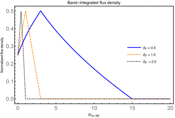
Figure 8: The analytical and normalized band-integrated flux density (given by Eq. (20) in Appendix SE.3) versus normalized time, $t/t_{\rm m-WI}=t^{\rm obs.}/t_{\rm m-WI}^{\rm obs.}(\theta_{\rm c})$; $t_{\rm m-WI}^{\rm obs.}(\theta_{\rm c})$ is the characteristic filament merging timescale (Eq. (8)). Shown here is the case “a" in the top panel of Figure 1 applied to CHIME’s detector with $\nu_{\rm max.}^{\rm det.}=800$ MHz and $\nu_{\rm min.}^{\rm det.}=400$ MHz and with $\nu_{\rm CSE,max.}^{\rm obs.}(0)=2\nu_{\rm max.}^{\rm det.}$ and $\nu_{\rm CSE,min.}^{\rm obs.}(0)=\nu_{\rm min.}^{\rm det.}/2$. Three different filament merging rates are shown ($\delta_{\rm m-WI}=0.5,1.0,2.0$) with the filament size evolving in ime as $\lambda_{\rm F}(t)=\lambda_{\rm e-WI}\times(1+t/t_{\rm m-WI})^{\delta_{\rm m-WI}}$ (Eq. (• ‣ SC.2)).

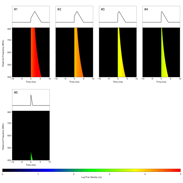
Figure 9: Same as in Figure 3 for the chunks listed in Table 9.

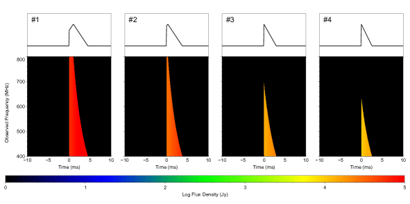
Figure 10: Same as in Figure 3 for the chunks listed in Table 10.

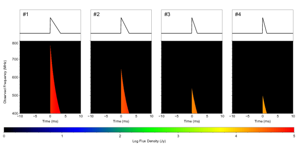
Figure 11: Same as in Figure 3 for the chunks listed in Table 11.

Figure 3 is the frequency-time plot (“waterfall" plot; Appendix SE.5) for the simulation shown in Table 2. The band(frequency)-summed flux density is in the upper sub-panels and matches the analytically derived one (Appendix SE.3 and Figure 8). Figures 9 and 10 show waterfall plots for the repeating FRBs listed in Tables 9 and 10. Figure 11 shows an example where the maximum CSE frequency falls within the detector’s band (here CHIME); see Table 11 for the corresponding simulations. Our model can reproduce the cases in the upper panels in Figure 1 and Figure 7.

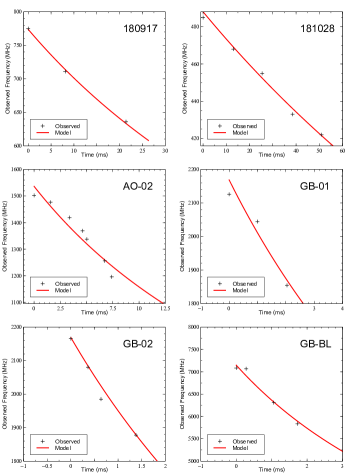
Figure 2: Sub-pulse frequency drifting fits: The two top panels show fits (solid lines) to two of CHIME’s FRB 180814.J0422$+$73 repeats (the 180917 and 181028 bursts; CHIME/FRB Collaboration 2019a). The middle and bottom panels show fits to four of FRB 121102 bursts (the AO-02, GB-01 GB-02 and GB-BL bursts; Hessels et al. 2019). The fitting parameters are listed in Table 3 and discussed in §3.2.

Table 3: Drifting in repeating FRBs: Fits to frequency drifting in time for selected CHIME FRB 180814.J0422$+$73 and FRB 121102 bursts (see related Figure 2). Other parameters are kept to their fiducial values listed in Table 4.

FRB	$z$	$\theta_{\rm c}$	$\zeta_{\rm m-WI}$	Chunk
CHIME (18/09/17)a	0.1	0.012	2700	Tertiary
CHIME (18/10/28)a	0.1	0.016	5700	Tertiary
121102 (AO-02)b	0.2	0.008	1700	Secondary
121102 (GB-01)b	0.2	0.007	1000	Secondary
121102 (GB-02)b	0.2	0.007	700	Secondary
121102 (GB-BL)b	0.2	0.002	2100	Primary

^a See CHIME/FRB Collaboration (2019a).
^b See Hessels et al. (2019).

4 Discussion

4.1 Rate

Assuming that the progenitors of ICM-QNe are old massive NSs, we estimate the ICM-QN occurrence rate. Slowly rotating, massive NSs are the most likely to experience quark deconfinement via nucleation and undergo a QN phase. We count only NSs with birth periods greater than $\sim 100$ ms and stellar progenitors with masses 20-40 M_☉. We use a lognormal initial magnetic field distribution (mean of 12.5 and standard deviation of 0.5) and a normal distribution for initial period (mean of 300 ms and standard deviation of 150 ms); from Faucher-Giguère & Kaspi (2006). We assume that ICM-QNe occur after a nucleation timescale of $\sim 10^{8}$ years.

Integration of the initial mass function (Salpeter 1955) and the initial period distribution (assuming period and magnetic field are independent) gives $\sim$ 10% of all neutron stars as QN candidates in the ICM. For a galactic core-collapse SN rate of $\sim 1/50$ years, over $10^{10}$ years about $\sim 2\times 10^{8}$ NSs would have formed. This yields

$$r_{\rm FRB}\sim 2\times 10^{-3}\ {\rm yr}^{-1}\ ,$$ (14)

or a few FRBs per thousand year per galaxy, consistent with the observed rate (Champion et al. 2016; Petroff et al. 2019).

4.2 Predictions (also Appendix SG)

• “Periodicity" (Repeats vs “non-repeats"): All FRBs are repeats because every chunk emits an FRB beamed in a specific direction. Non-repeaters are a consequence of observing limitations when emission from the secondary and tertiary chunks is too faint or when the corresponding frequency is below the bandwidth (Eq. (29)). All FRBs, if viewed at the right angle, will appear periodic in time with period (Eq.(13)) set by the roughly constant angular separation between chunks (Eq. (4)). This “periodicity" may be washed out with a variation in chunks parametersf ($m_{\rm c}$ and $\Gamma_{\rm c}$) and/or in the ambient density ($n_{\rm amb.}^{\rm ns}$);

• The halo/ICM low dispersion measure (DM): Recent studies (Caleb et al. 2019; Ravi 2019) concluded that FRBs sources must repeat in order to account for the high FRB volumetric rate. This constraint is relaxed in our model given the low DM, and thus larger volume, of the ambient medium (galactic halo, ICM, IGM) and our estimated rate of FRBs ($\sim$ 10% of the core-collapse SN rate). Within uncertainties on the observed rate, our model is in the allowed region (Figure 2 in Caleb et al. 2019) with no need for sources to repeat;

• The solid angle effect: CHIME (sub-GHz) is more sensitive to higher angle chunks and should detect more FRBs per QN than ASKAP and Parkes (GHz) detectors (Eq. (33)). CHIME FRBs should be dimmer and will be associated with duration (burst width) on average longer (but with variations) than ASKAP and Parkes FRBs;

• Super FRBs: We expect detection of super FRBs (with fluence in the thousands to tens of thousands of Jy ms) from ICM-QNe due to chunks very close to the observer’s line-of-sight. Monster FRBs from IGM-QNe with a fluence in the millions of Jy ms, may be detected by LOFAR’s low-band antenna. FRBs from IGM-QNe (Appendix SG.2 and Table 15) are extremely rare.

4.3 Model’s limitations (also Appendix SH)

• Parameter fitting: Table 4 lists 13 parameters. In developing the model we varied all of the parameters in order to obtain reasonable values for them. It is a challenge to constrain all of them and we restrict our investigations to varying a few basic parameters; $m_{\rm c}$, $\Gamma_{\rm c}$ and $N_{\rm c}$. We also varied $n_{\rm amb.}^{\rm ns}$ which allowed us to explore the evolution of the QN chunks in different environments (the Galactic halo, the ICM and the IGM). Other parameters (related to the BI-WI instabilities) will need to be surveyed in future studies;

• Bunching mechanism: The exact mechanism for bunching is unclear. In Appendix SD.2 we speculate that bunching occurs in the periphery and along the Weibel filaments. Our reasoning is that bunching (and CSE) would not occur inside filaments where the currents reside and the magnetic field is weaker. Regardless, bunches emit the BI heating efficiently and promptly as CSE during the bunch merging phase;

• QN compact remnant as magnetars (and the FRB association): The QS is born with a surface magnetic field of $\sim 10^{14}$-$10^{15}$ G (Iwazaki 2005). During the QS spin-down, vortices (and their magnetic field) are expelled (Ouyed et al. 2004; Niebergal et al. 2010b) leading to X-ray activity similar to that of Soft $\gamma$-ray Repeaters (SGRs) and Anomalous X-ray Pulsars (AXPs) (Ouyed et al. 2007a, b). Thus FRB activity for magnetars (e.g. Metzger et al. 2017) would be applicable to a QN compact remnant. The coincidence and association between FRB 200428 and SGR 1935$+$2154 (Barthelmy et al. 2020; Scholz et al. 2020; CHIME/FRB Collaboration 2020; Witze 2020; Bochenek et al. 2020) may find an explanation in our model.

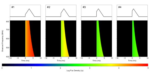
Figure 3: Waterfall plots for the chunks listed in Table 2 and detected in CHIME’s band. The palette shows flux density (Jy) in $\log$ scale. The upper sub-panels show the frequency-summed flux density over the detector’s frequency band $\nu_{\rm min.}^{\rm det.}\leq\nu^{\rm det.}\leq\nu_{\rm max.}^{\rm det.}$.

5 Conclusion

We present a model for FRBs involving old, slowly rotating and isolated NSs converting explosively to QSs (experiencing a QN event) in the ICM of galaxy groups and clusters. The NSs are embedded in the ICM when the QN occurs. The millions of QN chunks expand, due to heating by hadronic collisions with ambient protons, and become collisionless as they propagate away from the QN. The interaction of the collisonless chunks (the background plasma) with the ambient medium (the plasma beam), successively triggers the BI and WI yielding electron bunching and CSE with properties of repeating and non-repeating FRBs such as the GHz frequency, the milli-second duration and a fluence in the Jy ms range.

There are three classes of FRBs: those from ICM-QNe (i.e. galaxy group and cluster FRBs; §3), from galactic/halo-QNe (Appendix SF.2), and a third class, but the least likely one, corresponding to FRBs from IGM-QNes (Appendix SG.2) with frequencies at the lower limit of LOFAR’s low-band antenna. The distribution of NS natal kick velocities controls the ratio of galactic versus extra-galactic QNe (and their FRBs). We estimate an FRB rate of about 10% of that of ccSNe. Because of the low DM of the ambient medium, their volumetric rate can be explained without the need for the FRB sources to repeat (§4.2).

Our model can be used to probe collisionless plasma instabilities (see Appendix SI.1) and the QCD phase diagram (see Appendix SI.2). It has implications to Astrophysics (see Appendix SI.3) such as the existence of QSs forming mainly from old NSs exploding as QNe in the outskirts of galaxies. If the model is a correct representation of FRBs then it would strengthen the idea that QNe within a few years of a core-collapse SN of massive stars may be the origin of LGRBs (Ouyed al. 2020). Thus the same engine, the exploding NS, is responsible for GRBs and FRBs. For the FRBs case, the QN occurs hundreds of million of years after the SN.

We demonstrated that FRBs can be caused by a cataclysmic event, the QN. The millions of emitting chunks per QN is key with repeats a consequence of seeing multiple chunks coming in at different times and beamed in different directions. Single FRBs occur when only the primary chunk is within detector’s sensitivity. Our model relies on the feasibility of an explosive transition of a NS to a QS. While such a transition is indicated by analytical studies (Keränen et al. 2005; Vogt et al. 2004; Ouyed & Leahy 2009; Ouyed al. 2020) and by one-dimensional numerical simulations (Niebergal et al. 2010a; Ouyed, A et al. 2018a, b), detailed multi-dimensional simulations are required to confirm or refute it (Niebergal 2011; Ouyed, A 2018).

Data availability

The data underlying this article are available in the article and in its online supplementary material.

Supplementary online material.

Appendix SA Ejecta properties and statistics

As described in Ouyed & Leahy (2009), the QN ejecta breaks up into millions of chunks. Here we adopt $N_{\rm c}=10^{6}$ as our fiducial value for the number of fragments which yields a typical chunk mass of $m_{\rm c}=M_{\rm QN}/N_{\rm c}\simeq 10^{22.3}\ {\rm gm}\times M_{\rm QN,28.3}/N_{\rm c,6}$. The chunk’s Lorentz factor is taken to be constant with $\Gamma_{\rm c}=\Gamma_{\rm QN}=10^{2.5}$ corresponding to a fiducial QN ejecta’s kinetic energy $E_{\rm QN}=\Gamma_{\rm c}M_{\rm QN}c^{2}\simeq 5.7\times 10^{51}$ erg; i.e. roughly 1% of the conversion energy is converted to the kinetic energy of the QN ejecta; these fiducial values are listed in Table 4.

Below we summarize some general properties of the QN ejecta (see details in §2.1 and Appendix B.1 in Ouyed al. 2020). Hereafter, unprimed quantities are in the chunk’s reference frame while the superscripts “ns" and “obs." refer to quantities in the NS frame (i.e. the ambient medium) and the observer’s frame, respectively. The chunk’s Lorentz factor $\Gamma_{\rm c}$ does not vary in time, during the FRB phase, in our model. The transformation from the local NS frame to the chunk’s frame is given by $dt^{\rm ns}=\Gamma_{\rm c}dt$ while the transformations from the chunk’s frame to the observer’s frame (where the emitted light is being observed) are $dt^{\rm obs.}=(1+z)dt/D(\Gamma_{\rm c},\theta_{\rm c})$, $\nu^{\rm obs.}=D(\Gamma_{\rm c},\theta_{\rm c})\nu/(1+z)$ with $z$ the source’s redshift and $\theta_{\rm c}$ the viewing angle (the angle between the observer and chunk’s velocity vector); $D(\Gamma_{\rm c},\theta_{\rm c})$ is the chunk’s Doppler factor. We note the following:

• The chunks are equally spaced in solid angle $\Omega$ around the explosion site. Defining $N_{\theta}$ as the number of chunks per angle $\theta$, we write $dN_{\theta}/d\Omega=const.=N_{\rm c}/4\pi$ with $d\Omega=2\pi\sin{\theta}d\theta$ so that $dN_{\theta}/d\theta=(N_{\rm c}/2)\sin{\theta}\simeq(N_{\rm c}/2)\theta$ with $\theta_{\rm c}<<1$. Because $N_{\rm c}\pi\Delta\theta_{\rm c}^{2}=4\pi$ when the chunks first form, the average angular separation between them is

  $$\Delta\theta_{\rm s}=2\Delta\theta_{\rm c}=\frac{4}{N_{\rm c}^{1/2}}\simeq\frac{4\times 10^{-3}}{N_{\rm c,6}^{1/2}}\ ,$$ (15)

  yielding $\Delta\theta_{\rm s}\sim 1/\Gamma_{\rm c}$ for our fiducial value of $N_{\rm c}=10^{6}$ and $\Gamma_{\rm c}=10^{2.5}$.

  A simplistic geometry to visualize the spatial distribution is a 2-dimensional honeycomb (see Figure 4) with 1 primary (the $i=1$) chunk at $0\leq\theta_{\rm c}<\Delta\theta_{\rm c}$ and $6\times(i-1)$ chunks for subsequent, and concentric, “rings" (with $i\geq 2$; i.e. 6 secondary chunks, 12 tertiary chunks etc..). In this geometry the range and mean angle of the primary (P), secondary (S) and tertiary (T) chunks are

  $$0 \leq\theta_{\rm P}<\Delta\theta_{\rm c}\ ,\quad\bar{\theta}_{\rm P}=\frac{\int_{0}^{\Delta\theta_{\rm c}}\theta^{2}d\theta}{\int_{0}^{\Delta\theta_{\rm c}}\theta d\theta}=\frac{4}{3N_{\rm c}^{1/2}}$$

  $$\Delta\theta_{\rm c} \leq\theta_{\rm S}<3\Delta\theta_{\rm c}\ ,\quad\bar{\theta}_{\rm S}=\frac{\int_{\Delta\theta_{\rm c}}^{3\Delta\theta_{\rm c}}\theta^{2}d\theta}{\int_{\Delta\theta_{\rm c}}^{3\Delta\theta_{\rm c}}\theta d\theta}=\frac{28}{9N_{\rm c}^{1/2}}$$

  $$3\Delta\theta_{\rm c} \leq\theta_{\rm T}<5\Delta\theta_{\rm c}\ ,\quad\bar{\theta}_{\rm T}=\frac{\int_{3\Delta\theta_{\rm c}}^{5\Delta\theta_{\rm c}}\theta^{2}d\theta}{\int_{3\Delta\theta_{\rm c}}^{5\Delta\theta_{\rm c}}\theta d\theta}=\frac{49}{6N_{\rm c}^{1/2}}\ .$$ (16)

  We see that $\bar{\theta}_{\rm S}\simeq 2.3\bar{\theta}_{\rm P}$ and $\bar{\theta}_{\rm T}\sim 6\bar{\theta}_{\rm P}$;

• Because $\Gamma_{\rm c}^{2}>>1$ and $\theta_{\rm c}<<1$ applies here, we write the Doppler factor as $D_{\rm c}(\Gamma_{\rm c},\theta_{\rm c})\simeq 2\Gamma_{\rm c}/f(\theta_{\rm c})$ with

  $$f(\theta_{\rm c})=1+(\Gamma_{\rm c}\theta_{\rm c})^{2}\ ,$$ (17)

  and $f(\theta_{\rm c})<<\Gamma_{\rm c}^{2}$. This yields:

  $$1\leq f(\theta_{\rm P})<1+0.4\frac{\Gamma_{\rm c,2.5}^{2}}{N_{\rm c,6}}$$

  $$1+0.4\frac{\Gamma_{\rm c,2.5}^{2}}{N_{\rm c,6}}\leq f(\theta_{\rm S})<1+3.6\frac{\Gamma_{\rm c,2.5}^{2}}{N_{\rm c,6}}$$

  $$1+3.6\frac{\Gamma_{\rm c,2.5}^{2}}{N_{\rm c,6}}\leq f(\theta_{\rm T})<1+10\frac{\Gamma_{\rm c,2.5}^{2}}{N_{\rm c,6}}\ ,$$ (18)

  and average values

  $$f(\bar{\theta}_{\rm P})\sim 1+0.18\frac{\Gamma_{\rm c,2.5}^{2}}{N_{\rm c,6}}$$

  $$f(\bar{\theta}_{\rm S})\sim 1+0.97\frac{\Gamma_{\rm c,2.5}^{2}}{N_{\rm c,6}}$$

  $$f(\bar{\theta}_{\rm T})\sim 1+6.67\frac{\Gamma_{\rm c,2.5}^{2}}{N_{\rm c,6}}\ ;$$ (19)

• The change in $f(\theta_{\rm c})$ between two successive “rings" is $\Delta f_{i+1,i}^{\rm rings}=f(\theta_{\rm ring,i+1})-f(\theta_{\rm ring,i})=\Gamma_{\rm c}^{2}\times(\theta_{\rm ring,i+1}^{2}-\theta_{\rm ring,i}^{2})=\Gamma_{\rm c}^{2}\times(\theta_{\rm ring,i+1}-\theta_{\rm ring,i})(\theta_{\rm ring,i+1}+\theta_{\rm ring,i})$. Using $\theta_{\rm ring,i+1}=\theta_{\rm ring,i}+\Delta\theta_{\rm s}$ one finds

  $$\Delta f_{i+1,i}^{\rm rings}=1.6\times\frac{\Gamma_{\rm c,2.5}^{2}}{N_{\rm c,6}}\times(1+\frac{2\theta_{\rm ring,i}}{\Delta\theta_{\rm s}})\ ,$$ (20)

  with $\theta_{\rm ring,i}/\Delta\theta_{\rm s}=i$ for equally spaced“rings".

  The average change in the radial angle from one random chunk to another (i.e. the actual separation projected onto the radial direction; see Figure 4) with respect to the observer is $\Delta f_{i+1,i}^{\rm chunks}\simeq\Delta f_{i+1,i}^{\rm rings}/N_{i}$. The number of chunks per ring, of perimeter $2\pi\times(i\Delta\theta_{\rm s})$, is $N_{\rm i}=2\pi\times(i\Delta\theta_{\rm s}/\Delta\theta_{\rm s})=2\pi i$. Thus,

  $$\Delta f_{i+1,i}^{\rm chunks}\simeq 1.6\times\frac{\Gamma_{\rm c,2.5}^{2}}{N_{\rm c,6}}\times\frac{(1+2i)}{2\pi i}\sim\frac{1.6}{\pi}\times\frac{\Gamma_{\rm c,2.5}^{2}}{N_{\rm c,6}}\ ,$$ (21)

  where the last expression applies for higher $i>\sim 2$. Because the chunks are not precisely equally spaced, the variation in $f(\theta_{\rm c})$ between chunks is somewhat variable.

Appendix SB Chunk expansion and the onset of the collisionless plasma regime

We define $R_{\rm c}$ as the chunk’s radius. The photon transparency radius for the chunk is $R_{\rm c,opt.}\simeq 2.2\times 10^{10}\ {\rm cm}\times m_{\rm c,22.3}^{1/2}\kappa_{\rm c,-1}^{1/2}$ with $m_{\rm c,22.3}$ its mass (in units of $10^{22.3}$ gm) and $\kappa_{\rm c,-1}$ its opacity (in units of 0.1 cm² gm^-1). For $R_{\rm c}>R_{\rm c,opt.}$, the thermal and dynamical evolution of the chunk is governed by heating ($Q_{\rm HH}$) from hadronic collisions with the ambient medium and thermalization due to electron Coulomb collisions followed by adiabatic cooling (PdV expansion). The heat transfer equations describing the time evolution of the chunk’s radius $R_{\rm c}$ and its temperature $T_{\rm c}$ are

$$\frac{dR_{\rm c}}{dt} =c_{\rm c,s}$$

$$C_{\rm v}\frac{dT_{\rm c}}{dt} =Q_{\rm HH}-p_{\rm c}\frac{dV_{\rm c}}{dt}\ ,$$ (22)

where $c_{\rm c,s}=\sqrt{\gamma_{\rm ad.}k_{\rm B}T_{\rm c}/\mu_{\rm e}m_{\rm H}}$ is the chunk’s sound speed, $p_{\rm c}=n_{\rm c}k_{\rm B}T_{\rm c}$ its pressure, $V_{\rm c}=(4\pi/3)R_{\rm c}^{3}$ its volume and $C_{\rm V}=(m_{\rm c}/m_{\rm H})\times(3k_{\rm B}/2)$ its heat capacity. The adiabatic index we take to be $\gamma_{\rm ad.}=5/3$ with a mass per electron $\mu_{\rm e}=2$; $k_{\rm B}$ is the Boltzmann constant.

Equations above can be combined into

$$\frac{dc_{\rm c,s}^{2}}{dt} =\frac{2\gamma_{\rm ad.}Q_{\rm HH}}{3\mu_{\rm e}m_{\rm c}}-2\frac{c_{\rm c,s}^{3}}{R_{\rm c}}\ .$$ (23)

The optical depth to hadronic collisions is $\tau_{\rm HH}=n_{\rm c}\sigma_{\rm HH}R_{\rm c}=3m_{\rm c}\sigma_{\rm HH}/m_{\rm H}4A_{\rm c}<<1$ where $A_{\rm c}=\pi R_{\rm c}^{2}$ is the chunk’s area and $n_{\rm c}=3m_{\rm H}/4\pi R_{\rm c}^{3}m_{\rm H}$ its baryon number density. Thus, heating due to hadronic collisions can be written as $Q_{\rm HH}=\tau_{\rm HH}\times(\Gamma_{\rm c}m_{\rm H}c^{2})\times(A_{\rm c}\Gamma_{\rm c}n_{\rm amb.}^{\rm ns}c)=m_{\rm c}\sigma_{\rm HH}\Gamma_{\rm c}^{2}n_{\rm amb.}^{\rm ns}c^{3}$. The term $A_{\rm c}\Gamma_{\rm c}n_{\rm amb.}^{\rm ns}c$ is the number of ambient protons swept-up by the chunk per unit time; here $c$ is the light speed. This yields

$$Q_{\rm HH}\simeq 5.4\times 10^{28}\ {\rm erg\ s}^{-1}\times m_{\rm c,22.3}\sigma_{\rm HH,-27}\Gamma_{\rm c,2.5}^{2}n^{\rm ns}_{\rm amb.,-3}\ ,$$ (24)

where $\sigma_{\rm HH,-27}$ is the proton hadronic collision cross-section in units of milli-barns (e.g. Letaw et al. 1983; Tanabashi et al. 2018). Eq. (23) becomes

$$\frac{dc_{\rm c,s}^{2}}{dt} =q_{\rm HH}-2\frac{c_{\rm c,s}^{3}}{R_{\rm c}}\ ,$$ (25)

where $q_{\rm HH}=2\gamma_{\rm ad.}Q_{\rm HH}/3\mu_{\rm e}m_{\rm c}\simeq 1.5\times 10^{6}\times\sigma_{\rm HH,-27}\Gamma_{\rm c,2.5}^{2}n_{\rm amb.,-3}^{\rm ns}$ is the specific heating term due to hadronic collisions.

The solution of the system above is $R_{\rm c}(t)=R_{\rm c,0}(t/t_{0})^{3/2}$ and $c_{\rm c,s}(t)=c_{\rm c,s,0}(t/t_{0})^{1/2}$ with $c_{\rm c,s,0}=3R_{\rm c,0}/2t_{\rm 0}$ and $t_{\rm 0}=(27R_{\rm c,0}^{2}/2q_{\rm HH})^{1/3}$. For $R_{\rm c,0}=R_{\rm c,opt.}$, we get

$$t_{0}\simeq 1.6\times 10^{5}\ {\rm s}\times\left(\frac{m_{\rm c,22.3}\kappa_{\rm c,-1}}{\sigma_{\rm HH,-27}\Gamma_{\rm c,2.5}^{2}n_{\rm amb.,-3}^{\rm ns}}\right)^{1/3}\ .$$ (26)

The initial chunk temperature, found from $k_{\rm B}T_{0}=\mu_{\rm e}m_{\rm H}c_{\rm c,s,0}^{2}$, is

$$T_{0}\simeq 10^{3}\ {\rm K}\times(m_{\rm c,22.3}\kappa_{\rm c,-1})^{1/3}\times\left(\sigma_{\rm HH,-27}\Gamma_{\rm c,2.5}^{2}n_{\rm amb.,-3}^{\rm ns}\right)^{2/3}\ .$$ (27)

The chunk becomes collisionless when the electron Coulomb collision length inside the chunk, $\lambda_{\rm Coul.,e}\simeq 1.1\times 10^{4}\ {\rm cm}\times T_{\rm c,e}^{2}/n_{\rm c,e}$ (Richardson (2019) with a Coulomb parameter $\ln{\Lambda}=20$; e.g. Lang 1999) is of the order of the chunk’s radius $R_{\rm c}$. Setting $\lambda_{\rm Coul.,e}(t_{\rm cc})=R_{\rm c}(t_{\rm cc})$ with $n_{\rm c}(t)=3m_{\rm c}/4\pi R_{\rm c}(t)^{3}m_{\rm H}$, $R_{\rm c}(t)=R_{\rm c,0}(t/t_{0})^{3/2}$ and $T(t)=T_{0}(t/t_{0})$ yields

$$\frac{t_{\rm cc}}{t_{0}}\simeq 878.8\times T_{\rm 0,3}^{-2/5}\ ,$$ (28)

where the chunk’s initial temperature (when it becomes optically thin) is in units of $10^{3}$ K. The subscript “cc" stands for collisionless chunk.

The chunk’s temperature, radius and number density when it enters the collisionless regime are

$$T_{\rm cc} \simeq 8.8\times 10^{5}\ {\rm K}\times T_{\rm 0,3}^{3/5}\quad\simeq 8.8\times 10^{5}\ {\rm K}\times(m_{\rm c,22.3}\kappa_{\rm c,-1})^{1/5}(\sigma_{\rm HH,-27}\Gamma_{\rm c,2.5}^{2}{n_{\rm amb.,-3}^{\rm ns}})^{2/5}$$ (29)

$$R_{\rm cc} \simeq 5.9\times 10^{14}\ {\rm cm}\times\frac{m_{\rm c,22.3}^{1/2}\kappa_{\rm c,-1}^{1/2}}{T_{\rm 0,3}^{3/5}}\quad\simeq 5.9\times 10^{14}\ {\rm cm}\times\frac{(m_{\rm c,22.3}\kappa_{\rm c,-1})^{3/10}}{(\sigma_{\rm HH,-27}\Gamma_{\rm c,2.5}^{2}{n_{\rm amb.,-3}^{\rm ns}})^{2/5}}$$ (30)

$$n_{\rm cc} \simeq 14.6\ {\rm cm}^{-3}\times\frac{T_{\rm 0,3}^{9/5}}{m_{\rm c,22.3}^{1/2}\kappa_{\rm c,-1}^{3/2}}\quad\simeq 14.6\ {\rm cm}^{-3}\times\frac{m_{\rm c,22.3}^{1/10}}{\kappa_{\rm c,-1}^{9/10}}\times(\sigma_{\rm HH,-27}\Gamma_{\rm c,2.5}^{2}{n_{\rm amb.,-3}^{\rm ns}})^{6/5}\ .$$ (31)

This yields an estimate of the chunk electron thermal speed $\beta_{\rm cc}=v_{\rm cc}/c=\sqrt{\gamma_{\rm ad.}k_{\rm B}T_{\rm cc}/m_{\rm e}c^{2}}$ as

$$\beta_{\rm cc}\simeq 1.6\times 10^{-2}\times T_{\rm 0,3}^{3/10}\quad\simeq 1.6\times 10^{-2}\times(m_{\rm c,22.3}\kappa_{\rm c,-1})^{1/10}(\sigma_{\rm HH,-27}\Gamma_{\rm c,2.5}^{2}{n_{\rm amb.,-3}^{\rm ns}})^{1/5}\ .$$ (32)

The time, since the QN event, it takes the chunk to become collisionless in the chunk frame is:

$$t_{\rm cc}\simeq 1.7\times 10^{3}\ {\rm days}\times T_{\rm 0,3}^{-2/5}\times\left(\frac{m_{\rm c,22.3}\kappa_{\rm c,-1}}{\sigma_{\rm HH,-27}\Gamma_{\rm c,2.5}^{2}n_{\rm amb.,-3}^{\rm ns}}\right)^{1/3}\quad\simeq 1.7\times 10^{3}\ {\rm days}\times\frac{(m_{\rm c,22.3}\kappa_{\rm c,-1})^{1/5}}{(\sigma_{\rm HH,-27}\Gamma_{\rm c,2.5}^{2}{n_{\rm amb.,-3}^{\rm ns}})^{3/5}}\ ,$$ (33)

which is $t_{\rm cc}^{\rm obs.}=(1+z)t_{\rm cc}/D(\Gamma_{\rm c},\theta_{\rm c})$ in the observer’s frame with the Doppler factor $D(\Gamma_{\rm c},\theta_{\rm c})\simeq 2\Gamma_{\rm c}/f(\theta_{\rm c})$ and $f(\theta_{\rm c})$ given by Eq. (17). I.e.,

$$t_{\rm cc}^{\rm obs.}\simeq 2.6\ {\rm days}\times\frac{(1+z)f(\theta_{\rm c})}{\Gamma_{\rm c,2.5}}\times T_{\rm 0,3}^{-2/5}\times\left(\frac{m_{\rm c,22.3}\kappa_{\rm c,-1}}{\sigma_{\rm HH,-27}\Gamma_{\rm c,2.5}^{2}n_{\rm amb.,-3}^{\rm ns}}\right)^{1/3}\quad\simeq 2.6\ {\rm days}\times\frac{(1+z)f(\theta_{\rm c})}{\Gamma_{\rm c,2.5}}\times\frac{(m_{\rm c,22.3}\kappa_{\rm c,-1})^{1/5}}{(\sigma_{\rm HH,-27}\Gamma_{\rm c,2.5}^{2}{n_{\rm amb.,-3}^{\rm ns}})^{3/5}}\ .$$ (34)

In the NS (ambient) frame $t_{\rm cc}^{\rm ns}=\Gamma_{\rm c}t_{cc}\sim$ 1472.8 yr.

SB.1 The ionization stage

The chunk becomes ionized at time $t=t_{\rm ic}$ when hadronic collisions heats it up to $T_{\rm ic}=13.6$ eV prior to becoming collisionless; “ic" stands for ionized chunk. For $t_{\rm ic}\leq t<t_{\rm cc}$, we can associate a thermal Bremsstrahlung (TB) luminosity to the chunk $L_{\rm TB}(t)=1.43\times 10^{-27}n_{\rm c,e}(t)n_{\rm c,i}(t)T_{\rm c}(t)^{1/2}V_{\rm c}(t)Z^{2}g$ (e.g. Lang 1999). In our case we have $Z=1$, $n_{\rm c,e}=n_{\rm c,i}=n_{\rm c,0}(t/t_{0})^{-9/2}$ (with $n_{\rm c,0}=3m_{\rm c}/4\pi R_{\rm c,opt.}^{3}m_{\rm H}$), $T_{\rm c}(t)=T_{0}(t/t_{0})$ and, $V_{\rm c}=(4\pi/3)R_{\rm c}(t)^{3}$ the chunk’s volume; $g\simeq 1.2$ is the frequency averaged Gaunt factor. We get

$$L_{\rm TB}(t)\simeq 1.7\times 10^{35}\ {\rm erg\ s}^{-1}\times\frac{m_{\rm c,22.3}^{1/2}T_{\rm 0,3}^{1/2}}{\kappa_{\rm c,-1}^{3/2}}\times\left(\frac{t}{t_{0}}\right)^{-4}\ .$$ (35)

Setting $T_{\rm ic}=T_{0}(t_{\rm ic}/t_{0})$ gives us

$$\frac{t_{\rm ic}}{t_{0}}\simeq 157.8\times T_{\rm 0,3}^{-1}\ ,$$ (36)

and a maximum (i.e. initial) thermal Bremsstrahlung luminosity (at $t=t_{\rm ic}$)

$$L_{\rm TB,max.}\simeq 2.7\times 10^{26}\ {\rm erg\ s}^{-1}\times\frac{m_{\rm c,22.3}^{1/2}T_{\rm 0,3}^{9/2}}{\kappa_{\rm c,-1}^{3/2}}\ .$$ (37)

The above is negligible compared to heating from hadronic collision ($Q_{\rm HH}$; see Eq.(24)). When the chunk enters the collisionless phase at $t_{\rm cc}$, with $t_{\rm cc}/t_{\rm ic}\simeq(878.8/157.8)\times T_{\rm 0,3}^{3/5}$, the thermal Bremsstrahlung is even smaller with $L_{\rm TB}(t_{\rm cc})\simeq 10^{-3}\times L_{\rm TB}(t_{\rm ic})$. Although negligible compared to hadronic heating, thermal Bremsstrahlung (when $t_{\rm ic}\leq t\leq t_{\rm cc}$) is boosted to a maximum observed luminosity

$$L_{\rm TB,max.}^{\rm obs.}\simeq 4.4\times 10^{37}\ {\rm erg\ s}^{-1}\times\frac{1}{(1+z)^{2}f(\theta_{\rm c})^{4}}\times\sigma_{\rm HH,-27}^{3}\Gamma_{\rm c,2.5}^{10}m_{\rm c,22.3}^{2}{n_{\rm amb.,-3}^{\rm ns}}^{3}\ .$$ (38)

The TB phase lasts for $t_{\rm cc}^{\rm obs.}$ which is of the order of days for fiducial parameter values.

Appendix SC Interaction with the ambient plasma: the relevant instabilities

SC.1 The background plasma and the beam

We use results from Particle-In-Cell (PIC) and laboratory studies of instabilities in inter-penetrating plasmas, to identify the relevant plasmas:

• The background ${\it(e^{-},p^{+})}$ plasma: is the collisionless ionized chunk material dissociated into hadronic constituents during its early evolution when interacting with the ambient medium in the close vicinity of the QN site. When the chunk becomes collisionless, its radius, baryon number density and temperature are (see Eqs. (29), (30) and ((31) in Appendix SB): $R_{\rm cc}\sim 10^{15}$ cm, $n_{\rm cc}\sim 10$ cm^-3 and $T_{\rm cc}\sim 0.1$ keV, respectively. Here, the subscript “cc" stands for “collisionless chunk" defining the start of the collisionless phase. This occurs at time $t_{\rm cc}^{\rm obs.}\simeq 2.6\ {\rm days}\times(1+z)f(\theta_{\rm c})\times(m_{\rm c,22.3}\kappa_{\rm c,-1})^{1/5}/(\sigma_{\rm HH,-27}^{3}\Gamma_{\rm c,2.5}^{11}({n_{\rm amb.,-3}^{\rm ns}})^{3})^{1/5}$ after the QN (Eq.(33));

• The ${\it(e^{-},p^{+})}$ plasma beam: is the ionized ambient medium (e.g. ICM) incident on the QN chunks as they travel. Its baryon number density is $n_{\rm amb.}^{\rm ns}$ in the NS frame.

The parameters that define the regimes of collisionless instabilities are:

• Ultra-relativistic motion: $\Gamma_{\rm c}>>1$;

• Density ratio: The beam (ambient medium) to background plasma (collisionless chunk) baryon number density ratio in the chunk frame is

  $$\alpha_{\rm cc}=\frac{\Gamma_{\rm c}n_{\rm amb.}^{\rm ns}}{n_{\rm cc}}=10^{-1.5}\frac{\Gamma_{\rm c,2.5}{n_{\rm amb.,-3}^{\rm ns}}}{n_{\rm cc,1}}\ .$$ (39)

  From $n_{\rm cc}\propto{\Gamma_{\rm c}^{12/5}(n_{\rm amb.}^{\rm ns})}^{6/5}$ (Eq. (30)), we have $\alpha_{\rm cc}\propto{\Gamma_{\rm c}^{-7/5}(n_{\rm amb.}^{\rm ns})}^{-1/5}$ which is weakly dependent on $n_{\rm amb.}^{\rm ns}$ but rather more on the chunk’s Lorentz factor $\Gamma_{\rm c}$;

• Magnetization ($B_{\rm cc}^{2}/8\pi n_{\rm cc}m_{\rm H}c^{2}$): The evolution of the chunk’s magnetic field is estimated by flux conservation $B_{\rm NS}(4\pi R_{\rm NS}^{2}/N_{\rm c})=B_{\rm cc}\pi R_{\rm cc}^{2}$ where $B_{\rm NS}$ and $R_{\rm NS}$ are the NS’s magnetic field and radius, respectively. This gives

  $$B_{\rm cc}\simeq 1.3\times 10^{-11}\ {\rm G}\times\frac{B_{\rm NS,12.5}}{N_{\rm c,6}}\times\left(\frac{R_{\rm NS,6}}{R_{\rm cc,15}}\right)^{2}\ .$$ (40)

  With $n_{\rm cc}\sim 10$ cm^-3 (see Eq. (30)), one has $B_{\rm cc}^{2}/8\pi<<n_{\rm cc}m_{\rm H}c^{2}$ when the chunk becomes collisionless, effectively becoming a non-magnetized plasma when experiencing the inter-penetrating instabilities discussed below.

SC.2 The instabilities

The above parameter ranges imply that at the onset of the collisionless stage, the Buneman instability (BI) dominates the dynamics (e.g. Table 1 and Figure 5 in Bret 2009). The BI induces an anisotropy in the chunk’s electron temperature distribution, triggering the thermal Weibel instability (WI; Weibel 1959), which has the effect of isotropizing the temperature. The thermal WI requires only a temperature anisotropy to exist and is beam-independent. The Weibel filamentation instability (FI) on the other hand requires a beam to exist (Fried 1959). However, the FI dominates only when $\alpha_{\rm cc}\sim 1$ (see Figure 5 in Bret 2009), which is not the case here because we have $\alpha_{\rm cc}<<1$ as expressed in Eq. (39).

The beam (i.e. the ICM plasma) triggers the longitudinal BI (with wave vector aligned with the beam). This creates the needed anisotropy since the BI yields efficient heating of electrons in the longitudinal direction (parallel to the beam). The scenario is a parallel plasma temperature which exceeds the perpendicular plasma temperature, allowing the thermal WI to act (even in the weak anisotropy case). During the development of the WI, the beam continues to feed the BI by continuous excitation of electrostatic waves.

These two instabilities are discussed in more detail below. We define $\beta_{\parallel}=v_{\parallel}/c$ and $\beta_{\perp}=v_{\perp}/c$, where $c$ is the light speed, as the chunk electron’s speed in the direction parallel and perpendicular to the beam, respectively. When a QN chunk becomes collisionless, it has $\beta_{\parallel}=\beta_{\perp}=\beta_{\rm cc}\sim 10^{-2}$ (Eq. (32)):

• The Buneman Instability (BI) is an electro-static instability (i.e. excitations of electrostatic waves). It is an electron-ion two-stream instability caused by the resonance between the plasma oscillation of the chunk electrons and plasma oscillation of the ambient medium protons (Buneman 1958, 1959). In our case, it arises when the relative drift velocity between the beam (i.e. ICM) protons and the plasma (i.e. chunk) electrons exceeds the chunk’s electron thermal velocity. Its wave vector is parallel to the beam propagation direction and generates stripe-like patterns (density stripes perpendicular to the beam; e.g. Bret et al. 2010). The BI gives rise to rapid electron heating (e.g. Davidson 1970, 1974; Hirose 1978) by transferring a percentage of the beam’s kinetic energy into thermal (electron) energy of the background plasma (here the QN chunk) by turbulent (electric field) heating. The end result is an increase in $\beta_{\parallel}$ with $\beta_{\perp}$ unchanged. The wavelength of the dominant mode is

  $$\lambda_{\rm BI}=\alpha_{\rm cc}\times\frac{c}{\nu_{\rm p,e}}\ ,$$ (41)

  where $\nu_{\rm p,e}=(4\pi e^{2}n_{\rm cc,e}/m_{\rm e})^{1/2}\simeq(9\ {\rm kHz})\times n_{\rm cc}^{1/2}$ is the non-relativistic electron plasma frequency of the chunk and $n_{\rm cc,e}=n_{\rm cc}$ the chunk’s electron density; $m_{\rm e}$ and $e$ are the electron’s mass and charge, respectively. The e-folding growth timescale is

  $$t_{\rm BI}=\frac{2^{4/3}}{3^{1/2}}\left(\frac{m_{\rm p}}{m_{\rm e}}\right)^{1/3}\times\frac{1}{\nu_{\rm p,e}}\simeq\frac{17.8}{\nu_{\rm p,e}}\simeq\frac{0.63\ {\rm ms}}{n_{\rm cc,1}^{1/2}}\ ,$$ (42)

  where $m_{\rm p}$ is the proton mass. The above is much shorter than the chunk’s crossing time $R_{\rm cc}/c\sim 3.3\times 10^{4}\ {\rm s}\times R_{\rm cc,15}$ allowing plenty of time for the BI to grow and saturate locally throughout the collisionless chunk.

  BI heating occurs by transferring beam electron energy to heating chunk’s electrons. BI saturation occurs much before the beam kinetic energy is depleted because of trapping of electrons by turbulence; i.e. BI saturates at a particular electric field (e.g. Hirose 1978). The heat gain by the chunk’s electrons is $Q_{\rm BI}=(\zeta_{\rm BI}\Gamma_{\rm c}m_{\rm e}c^{2})\times(A_{\rm cc}\Gamma_{\rm c}n_{\rm amb.}^{\rm ns}c)$, where $A_{\rm cc}=\pi R_{\rm cc}^{2}$, or

  $$Q_{\rm BI}\simeq 7.6\times 10^{35}\ {\rm erg\ s}^{-1}\times\zeta_{\rm BI,-1}\Gamma_{\rm c,2.5}^{2}R_{\rm cc,15}^{2}n_{\rm amb.,-3}^{\rm ns}\ ,$$ (43)

  expressed in terms of the BI saturation, parameter $\zeta_{\rm BI}$ (here free). It is the fraction of the electrons kinetic energy (in the beam) converted to an electrostatic field and subsequently to heating the chunk’s electrons (to increasing $\beta_{\parallel}$). At saturation, the electron energy gain is $\sim$ 10% of the beam electron kinetic energy; the protons energy gain is much less than that of chunk electrons (e.g. Dieckmann et al. (2012); Moreno et al. (2018)).

• The thermal Weibel Instability (WI) is an electro-magnetic instability which occurs in plasmas with an anisotropic electron temperature distribution (Weibel 1959; see Fried 1959 for Weibel FI). Its wave vector is perpendicular to the high temperature axis which corresponds to the beam propagation direction induced by the BI heating. The WI can efficiently generate magnetic fields. The corresponding currents are in the direction parallel to the beam with the resulting magnetic field perpendicular to it. As the BI accelerates electrons (increasing $\beta_{\parallel}$), the WI heats up the chunk’s electrons via particle scattering by the generated magnetic field, accelerating them in the transverse direction (increasing $\beta_{\perp}$), as to reduce the BI-induced thermal anisotropy.

  The WI was studied theoretically in the non-relativistic and relativistic regimes (Weibel 1959; Fried 1959; Yoon & Davidson 1987; see also Medvedev & Loeb 1999; Gruzinov 2001) and numerically using PIC simulations (e.g. Kato 2007; Spitkovsky 2008; Nishikawa et al. 2009). Its key phases which are of relevance to our model for FRBs are:

  (i) Electron-WI (e-WI): Because of the small inertia, chunk electrons dominate the dynamics setting the characteristic correlation length of magnetic field and its growth rate. We use Eqs. (A4a) and (A4b) in Medvedev & Loeb (1999), which describe the mode with the largest growth rate, valid for $\beta_{\perp}=v_{\perp}/c<<1$ and for $\beta_{\parallel}=v_{\parallel}/c$ which is arbitrary in our model. In the notation of Medvedev & Loeb (1999), our scenario corresponds to $\hat{\gamma}=1$ and $G(\beta_{\perp})=(2\beta_{\perp})^{-1}\ln{(1+\beta_{\perp})/(1-\beta_{\perp})}\simeq(2\beta_{\perp})^{-1}\ln{(1+2\beta_{\perp})}\simeq 1$. The wavenumber $k_{\rm max.}$ and growth rate $\Gamma_{\rm max.}$ of the dominant mode are, respectively,

  $$k_{\rm max}^{2}c^{2}\simeq\nu_{\rm p,e}^{2}\frac{\beta_{\parallel}}{\sqrt{2}\gamma_{\parallel}\beta_{\perp}}\left(1-\frac{\beta_{\parallel}\beta_{\perp}}{\sqrt{2}}-\frac{\sqrt{2}\beta_{\perp}}{\beta_{\parallel}}\right)\quad\quad\quad\Gamma_{\rm max.}^{2}\simeq\nu_{\rm p,e}^{2}\frac{\beta_{\parallel}^{2}}{\gamma_{\parallel}}\left(1-2\sqrt{2}\frac{\beta_{\perp}}{\beta_{\parallel}}\right)\ ,$$ (44)

  where $\nu_{\rm p,e}$ is the electron plasma frequency. The above shows that the WI saturates when $\beta_{\parallel}=2\sqrt{2}\beta_{\perp}$.

  The dominant wavelength in the non-relativistic regime (with $\gamma_{\parallel}=1$) is:

  $$\lambda_{\rm e-WI} \simeq\left(\frac{\beta_{\perp}}{\beta_{\parallel}}\right)^{1/2}\times\frac{c}{\nu_{\rm p,e}}=\beta_{\rm WI}^{1/2}\times\frac{c}{\nu_{\rm p,e}}$$

  $$\simeq 3.5\times 10^{5}\ {\rm cm}\times\frac{\beta_{\rm WI,-1}^{1/2}}{n_{\rm cc,1}^{1/2}}\ ,$$ (45)

  where we defined $\beta_{\rm WI}=\beta_{\perp}/\beta_{\parallel}<1$. From Eq. (44), we must have $\beta_{\parallel}>2\sqrt{2}\beta_{\perp}$ for the WI to be triggered. Hereafter we set $\beta_{\parallel}=10\beta_{\perp}$ (i.e. $\beta_{\rm WI}=\beta_{\perp}/\beta_{\parallel}=0.1$ as the fiducial value) with $\beta_{\perp}=\beta_{\rm cc}\sim 10^{-2}$ given by the initial conditions when the chunk first becomes collisionless (i.e. Eq.(32)).

  The WI current filament structures have a transverse width of the order of $\lambda_{\rm e-WI}$ and are elongated in the beam’s direction (Appendix SD.2 and Figure 6). This dominant mode grows on an e-folding timescale of

  $$t_{\rm e-WI} \simeq\frac{1}{\beta_{\parallel}}\times\frac{1}{\nu_{\rm p,e}}=\frac{\beta_{\rm WI}}{\beta_{\perp}}\times\frac{1}{\nu_{\rm p,e}}$$

  $$\simeq 0.35\ {\rm ms}\times\frac{\beta_{\rm WI,-1}}{\beta_{\rm cc,-2}}\times\frac{1}{n_{\rm cc,1}^{1/2}}\ \ .$$ (46)

  In the linear regime we estimate the saturation time of the e-WI, $t_{\rm e-WI,s}$, by setting $B_{\rm e-WI,s}=B_{\rm cc}e^{(t_{\rm e-WI,s}/t_{\rm e-WI})}$ with $B_{\rm e-WI,s}^{2}/8\pi\sim n_{\rm cc}m_{\rm e}c^{2}$ the magnetic field strength at saturation. This is equivalent to writing $\nu_{\rm B}\sim\nu_{\rm p,e}$ at e-WI saturation with here $\nu_{\rm B}=eB_{\rm e-WI,s}/m_{\rm e}c$, the electron cyclotron frequency at e-WI saturation. We get

  $$t_{\rm e-WI,s}\simeq\left(21.2+\ln{\frac{n_{\rm cc,1}^{1/2}}{B_{\rm cc,-11}}}\right)\times t_{\rm e-WI}\ ,$$ (47)

  with $B_{\rm cc}$ given in Eq. (40);

  (ii) Proton-WI (p-WI): After the e-WI stage, and still in the linear regime, follows the p-WI stage which grows more slowly than the e-WI, on timescales $t_{\rm p-WI}=\sqrt{m_{\rm p}/m_{\rm e}}t_{\rm e-WI}$. The magnetic field is further amplified to a saturation value $B_{\rm p-WI,s}=\sqrt{m_{\rm p}/m_{\rm e}}B_{\rm e-WI,s}$ (Bret et al. 2016 and references therein). The saturation time $t_{\rm p-WI,s}$ of the p-WI phase is found by setting $B_{\rm p-WI,s}=B_{\rm e-WI,s}\times e^{(t_{\rm p-WI,s}/t_{\rm p-WI,})}$. This gives $t_{\rm p-WI,s}=(m_{\rm p}/m_{\rm e})^{1/2}\ln{(\sqrt{m_{\rm p}/m_{\rm e}})}\times t_{\rm e-WI}$, or,

  $$t_{\rm p-WI,s}\sim 161\times t_{\rm e-WI}\ .$$ (48)

  SC.3 Non-linear regime: filament merging (m-WI)

  In the non-linear regime, following the saturation of the p-WI stage, the filaments start merging and grow in size increasing $\lambda_{\rm e-WI}$. The merging is a result of the attractive force between parallel currents (Lee & Lampe 1973; Frederiksen et al. 2004; Kato 2005; Medvedev et al. 2005; Milosavljevic & Nakar 2006). Recent theoretical (e.g. Achterberg et al. (2007)) and numerical (e.g. Takamoto et al. (2018)) studies suggest a slow and a complex merging process. PIC simulations of filament merging in 3-dimensions (Takamoto et al. (2018, 2019)) find that during filament merging: (a) Electrons are stochastically accelerated by the magnetic turbulence generated by the WI up to a Lorentz factor of $\gamma_{\rm e}\sim 10$; (b) this heating sustains the WI saturated magnetic field for at least hundreds of ion plasma oscillations. Relying on these studies, we set a typical merging timescale as

  $$t_{\rm m-WI} \simeq\frac{10^{2}\zeta_{\rm m-WI,2}}{\nu_{\rm p,p}}\simeq\frac{4.3\times 10^{3}\ \zeta_{\rm m-WI,2}}{\nu_{\rm p,e}}$$

  $$\simeq 0.15\ {\rm s}\times\frac{\zeta_{\rm m-WI,2}}{n_{\rm cc,1}^{1/2}}\ ,$$ (49)

  where $\nu_{\rm p,p}=\sqrt{m_{\rm p}/m_{\rm e}}\nu_{\rm p,e}$ is the proton plasma frequency and $\zeta_{\rm m-WI}=10^{2}$ a parameter which allows us to adjust the merging timescale. The time evolution of the filament size we consider to be a power law

  $$\lambda_{\rm F}(t)=\lambda_{\rm e-WI}\times\left(1+\frac{t}{t_{\rm m-WI}}\right)^{\delta_{\rm m-WI}}\ ,$$ (50)

  with $\lambda_{\rm F}(0)=\lambda_{\rm e-WI}$ the filament’s transverse size during the linear regime and $\delta_{\rm m-WI}>0$ (simulations suggest $\delta_{\rm m-WI}\sim 0.76$; e.g. Takamoto et al. (2019)). Hereafter we adopt $\delta_{\rm m-WI}=1$ as our fiducial value.

  Proton trapping and shock formation: The Weibel shock occurs when the protons are trapped by the growing filaments; i.e. when the filament size becomes of the order of the beam’s proton’s Larmor radius. The shock quickly converts the chunk’s kinetic energy to internal energy by sweeping ambient protons leading to full chunk slowdown and shutting off the BI-WI process.

We close this appendix by discussing a few points:

• Table 4 lists the parameters related to the BI and WI instabilities and the fiducial values we adopted in this work. For the BI we have $\zeta_{\rm BI}$ which is the percentage of the beam’s electron energy (in the chunk fame) converted by the BI to heating the chunk electrons. The WI-related parameters are: (i) $\beta_{\rm WI}=\beta_{\perp}/\beta_{\parallel}$, the ratio of transverse to longitudinal thermal speed of chunk electrons (Eq. (• ‣ SC.2)) at the onset of the WI; (ii) $\zeta_{\rm m-WI}$ the filament merging characteristic timescale (Eq. (SC.3)) and; (iii) $\delta_{\rm m-WI}$ the power index of the filament merging rate as given in Eq. (50);

• We adopt $\beta_{\parallel}=10\beta_{\perp}$ (i.e. $\beta_{\rm WI}=\beta_{\perp}/\beta_{\parallel}=0.1$) during the linear stages of the WI instability which keeps $\lambda_{\rm e-WI}$ constant. While $\beta_{\parallel}$ grows due to the BI, the WI increases $\beta_{\perp}$ accordingly, as to the keep $\beta_{\rm WI}$ constant. However, because $\lambda_{\rm BI}/\lambda_{\rm e-WI}=\alpha_{\rm cc}/\beta_{\rm WI}^{1/2}<<1$, the BI deposits energy (i.e. heats up and accelerates electrons) in layers that are much narrower than those of the WI;

• With $t_{\rm BI}\sim 17.8/\nu_{\rm p,e}$ and $t_{\rm e-WI}=(\beta_{\rm WI}/\beta_{\perp})/\nu_{\rm p,e}\sim 10/\nu_{\rm p,e}$ being of the same order, the BI heat deposited within $\lambda_{\rm BI}$ is quickly mixed into much larger scales given by $\lambda_{\rm e-WI}$;

• The Oblique mode instability (when both longitudinal and transversal waves components are present at the same time) dominates when $\alpha_{\rm cc}>(m_{\rm e}/m_{\rm p})\Gamma_{\rm c}$ (e.g. Bret 2009). In our case this translates to $n_{\rm amb.}^{\rm ns}>(m_{\rm e}/m_{\rm p})n_{\rm cc}\simeq 0.5\ {\rm cm}^{-3}\times n_{\rm cc,1}$. Since the ICM’s density is $n_{\rm amb.}^{\rm ns}<<1$, the BI will always dominate;

• The BI heat is partly converted to amplifying the magnetic field (i.e. to magnetic energy density $B_{\rm p-WI,s}^{2}$), partly to turbulence with energy density $\delta B_{\rm p-WI,s}^{2}$ and, to currents. During filament merging, electrons are accelerated by dissipation of turbulent energy and currents while the WI saturated magnetic field is preserved (Takamoto et al. 2018). The BI energy harnessed during the linear regime is $E_{\rm BI}\sim Q_{\rm BI}t_{\rm p-WI,s}$. With $Q_{\rm BI}$ given by Eq. (43) and $t_{\rm p-WI,s}$ given by Eqs. (48) and (• ‣ SC.2), respectively, we get

  $$E_{\rm BI}\simeq 4.4\times 10^{34}\ {\rm ergs}\times\zeta_{\rm BI,-1}\times\frac{\beta_{\rm WI,-1}}{\beta_{\rm cc,-2}}\times\frac{\Gamma_{\rm c,2.5}^{2}R_{\rm cc,15}^{2}{n_{\rm amb.,-3}^{\rm ns}}}{n_{\rm cc,1}^{1/2}}\ ;$$ (51)

• The top panel in Figure 5 is a schematic representation of the evolution of $\beta_{\parallel}$ during the linear and non-linear WI stages ($\beta_{\perp}=0.1\beta_{\parallel}$ follows the evolution of $\beta_{\parallel}$). The increase in $\beta_{\parallel}$ is due to the BI and proceeds until the end of the p-WI stage, when the magnetic field saturates. At this point the BI excitations are converted entirely to heating electrons with the consequence that $\beta_{\parallel}$ increases rapidly following p-WI saturation. The BI shuts off when $\gamma_{\parallel}\sim 2$ because it acts only when the relative drift between the beam electrons and the chunk protons (here $c$) exceeds the chunk’s electrons thermal speed. Despite the BI shutting-off, the electrons continue to be accelerated by magnetic turbulence and by current dissipation during filament merging yielding $\gamma_{\parallel}\sim\gamma_{\perp}\sim 10$ (Takamoto et al. 2018). As discussed below, the increase in electron Lorentz factor during the merging phase, provides conditions favorable for coherent synchrotron emission (CSE) to occur in the WI-amplified magnetic field layers of the chunk.

Appendix SD Coherent synchrotron emission (CSE)

A relativistic electron beam moving in a circular orbit can radiate coherently if the characteristic wavelength of the incoherent synchrotron emission (ISE), $\lambda_{\rm ISE}$, exceeds the length of the electron bunch $\lambda_{\rm b}$. The near field of the radiation from each electron overlaps the entire bunch structure, resulting in a coherent interaction yielding a CSE frequency $\nu_{\rm CSE}=c/\lambda_{\rm b}$. With $N_{\rm e,b}$ the number of electrons in a bunch, the intensity of CSE scales as $N_{\rm e,b}^{2}$ instead of $N_{\rm e,b}$ as in the incoherent case (Schiff 1946; Schwinger 1949; Motz 1951; Nodvick & Saxon 1954; Ginzburg & Syrovatskii 1965).

The total power per bunch is estimated as $N_{\rm e,b}^{2}(\nu F_{\nu})_{\nu_{\rm CSE}}$ where $F_{\nu}=(\sqrt{3}\nu_{\rm B}e^{2}/c)\times F(\nu/\nu_{\rm ISE})$ is the incoherent synchrotron frequency distribution (in erg s^-1 Hz^-1) at the characteristic frequency $\nu_{\rm ISE}=(3/2)\gamma_{\rm e}^{2}\nu_{\rm B}$ with $\nu_{\rm B}=eB/m_{\rm e}c$ the cyclotron frequency and $\gamma_{\rm e}$ the electrons’ Lorentz factor. At $\nu_{\rm CSE}\sim c/\lambda_{\rm b}<<\nu_{\rm ISE}$, we have $F(\nu/\nu_{\rm ISE})\sim 2.15(\nu/\nu_{\rm ISE})^{1/3}$ which gives a total power per bunch of

$$L_{\rm b}\simeq 3.3\times 10^{-29}\times N_{\rm e,b}^{2}\nu_{\rm CSE}^{2}\frac{1}{\gamma_{\rm e}^{2/3}}\left(\frac{\nu_{\rm B}}{\nu_{\rm CSE}}\right)^{2/3}\ .$$ (1)

This agrees within a factor of a few with expressions given in the literature (e.g. Murphy et a. 1997 and references therein). The spectrum of CSE is the same as the incoherent one except for the $N_{\rm e,b}$ boosting and a decrease in the maximum (peak) frequency.

SD.1 CSE properties in our model

During the linear phase of the WI (up to p-WI saturation), CSE is unlikely to occur because BI heating cannot yield relativistic electrons ($\gamma_{\rm CSE}<2$; see top panel in Figure 5). Furthermore, bunching cannot be induced by the BI during filament merging because the instability does not grow if the background (i.e. chunk) electrons are so hot ($\gamma_{\rm CSE}>2$) that their thermal velocity spread exceeds the drift velocity relative to the beam (i.e. streaming ambient) ions. Instead, bunching is related to (i.e. entangled with) the WI filaments and CSE is likely to be triggered during filament merging when electrons are accelerated by magnetic turbulence and current dissipation to $\gamma_{\rm CSE}>>1$.

SD.1.1 Frequency and duration

With $\nu_{\rm B}\sim\sqrt{m_{\rm p}/m_{\rm e}}\nu_{\rm p,e}$ after p-WI saturation and during the filament merging phase, we calculate the chunk’s magnetic field strength to be

$$B_{\rm p-WI,s}\sim 0.12\ {\rm G}\times n_{\rm cc,1}^{1/2}\ ,$$ (2)

and the characteristic ISE frequency to be $\nu_{\rm ISE}=3/2\times\gamma_{\rm CSE}^{2}\sqrt{m_{\rm p}/m_{\rm e}}\nu_{\rm p,e}$.

The CSE frequency, $\nu_{\rm CSE}(t)=c/\lambda_{\rm b}(t)$, evolves in time due to the scaling of the bunch size $\lambda_{\rm b}(t)$ with that of the WI filament $\lambda_{\rm F}(t)$ which is expressed in Eq. (50). We find the CSE frequency to decrease in time during the filament merging phase at a rate given by

$$\nu_{\rm CSE}(t)=\frac{c}{\lambda_{\rm b}(t)}=\nu_{\rm CSE}(0)\times\left(1+\frac{t}{t_{\rm m-WI}}\right)^{-\delta_{\rm m-WI}}\ ,$$ (3)

with $\delta_{\rm m-WI}>0$ and $\nu_{\rm CSE}(0)=c/\lambda_{\rm e-WI}$; $\lambda_{\rm e-WI}$ given by Eq. (• ‣ SC.2) is the filament’s transverse size during the linear phase.

Because $\nu_{\rm CSE}<<\nu_{\rm ISE}$ we set the initial (also the maximum) CSE frequency as

$$\nu_{\rm CSE}(0)=\delta_{\rm CSE}\nu_{\rm ISE}\ ,$$ (4)

with $\delta_{\rm CSE}<<1$. The CSE frequency decreases in time until it reaches the chunk’s plasma frequency $\nu_{\rm p,e}$ shutting-off emission. The range in CSE frequency from a collisionless QN chunk is thus

$$\nu_{\rm p,e}\leq\nu_{\rm CSE}\leq\nu_{\rm CSE}(0)=\delta_{\rm CSE}\nu_{\rm ISE}\ .$$ (5)

The duration of CSE is found from $\nu_{\rm p,e}=\nu_{\rm CSE}(0)\times(1+\Delta t_{\rm CSE}/t_{\rm m-WI})^{-\delta_{\rm m-WI}}$ giving us:

$$\Delta t_{\rm CSE}=\left(\left(642.7\delta_{\rm CSE,-1}\gamma_{\rm CSE,1}^{2}\right)^{\frac{1}{\delta_{\rm m-WI}}}-1\right)\times t_{\rm m-WI}\ ,$$ (6)

with $\delta_{\rm m-WI}=1.0$, $\delta_{\rm CSE}=0.1$ and $\gamma_{\rm CSE}=10$ the fiducial values listed in Table 4.

SD.1.2 Luminosity

Most of the BI-induced heat is harnessed during the linear regime and up until the start of filament merging. Once the electrons thermal energy becomes relativistic (with $\gamma_{\rm CSE}>2$), the BI shuts-off. Effectively, the electrostatic energy deposited by the BI inside the chunk during the linear regime is $E_{\rm BI}\simeq Q_{\rm BI}t_{\rm p-WI,s}$ (see Eq. (51)) where $t_{\rm p-WI,s}$ is the p-WI saturation timescale. This energy is converted by the WI to: (i) magnetic field amplification with $B_{\rm p-WI,s}\sim\sqrt{m_{\rm p}/m_{\rm e}}B_{\rm e-WI,s}$ at saturation; (ii) magnetic turbulence; (iii) currents. Filament merging converts about 2/3 of the BI energy (by turbulence acceleration and current dissipation) to accelerating electrons (e.g. Takamoto et al. (2018)). The energy gained by the chunk electrons during filament merging is re-emitted as CSE luminosity expressed as $L_{\rm CSE}\sim(2/3)E_{\rm BI}/t_{\rm m-WI}$:

$$L_{\rm CSE}\simeq 1.9\times 10^{35}\ {\rm ergs}\times\frac{\zeta_{\rm BI,-1}\beta_{\rm WI,-1}}{\zeta_{\rm m-WI,2}}\times\frac{\Gamma_{\rm c,2.5}^{2}R_{\rm cc,15}^{2}n_{\rm amb.,-3}^{\rm ns}}{\beta_{\rm cc,-2}}\ .$$ (7)

SD.2 Bunch geometry and CSE luminosity

As illustrated in Figure 6 here, the Weibel filament extend across the collisionless chunk with length $2R_{\rm cc}$. The initial filament’s diameter is $\lambda_{\rm F}(0)=\lambda_{\rm e-WI}$ as expressed in Eq. (• ‣ SC.2). Bunching would manifest itself in a narrow region around the Weibel filaments where the magnetic field amplification is expected to occur and not inside filaments where the currents reside and the magnetic field is weaker. In other words, a typical bunch, where CSE occurs, would resemble a cylindrical shell around the Weibel filament with initial thickness $\lambda_{\rm b}(0)$, initial area $A_{\rm b}(0)=2\pi\lambda_{\rm e-WI}\lambda_{\rm b}(0)$ and, extending across the chunk. We have

$$\lambda_{\rm b}(0)\simeq\delta_{\rm b}\times\lambda_{\rm e-WI}\ ,$$ (8)

and because the maximum CSE frequency is expressed as $\nu_{\rm CSE}(0)=c/\lambda_{\rm e-WI}=\delta_{\rm CSE}\nu_{\rm ISE}$ (see Eq.(4)), this implies

$$\delta_{\rm b}=\frac{4.9\times 10^{-3}}{\beta_{\rm WI,-1}^{1/2}\delta_{\rm CSE,-1}\gamma_{\rm CSE,1}^{2}}<<1.0\ .$$ (9)

During filament merging the filament’s diameter (and thus the associated bunch thickness $\lambda_{\rm b}(t)=\delta_{\rm b}\lambda_{\rm F}(t)$) increases in time as $\lambda_{\rm F}(t)=\lambda_{\rm e-WI}\times(1+t/t_{\rm m-WI})^{-\delta_{\rm m-WI}}$ (see Eq. (50)) with $t_{\rm m-WI}$, given by Eq. (SC.3), the characteristic filament merging timescale. There is one bunch per filament which implies that the total number of bunches per chunk is $N_{\rm b,T}=\pi R_{\rm cc}^{2}/\pi\lambda_{\rm F}(t)^{2}$ and decreases in time at a rate given by

$$N_{\rm b,T}(t)\simeq 9\times 10^{18}\times\frac{R_{\rm cc,15}^{2}n_{\rm cc,1}}{\beta_{\rm WI,-1}}\times\left(1+\frac{t}{t_{\rm m-WI}}\right)^{-2\delta_{\rm m-WI}}\ .$$ (10)

The corresponding number of electrons per bunch is $N_{\rm e,b}(t)=V_{\rm b}(t)n_{\rm cc}$ with $V_{\rm b}(t)=(2\pi\lambda_{\rm F}(t)\lambda_{\rm b}(t))\times 2R_{\rm cc}=\delta_{\rm b}\times(2\pi\lambda_{\rm F}(t)^{2})\times 2R_{\rm cc}$ the volume. Thus

$$N_{\rm e,b}(t)\simeq 1.4\times 10^{26}\times R_{\rm cc,15}\times(\delta_{\rm b,-2}\beta_{\rm WI,-1})\times\left(1+\frac{t}{t_{\rm m-WI}}\right)^{+2\delta_{\rm m-WI}}\ .$$ (11)

The luminosity per bunch $L_{\rm b}(t)$ is given by inserting Eq. (11) into Eq. (1) with $\nu_{\rm B}\simeq\sqrt{m_{\rm p}/m_{\rm e}}\nu_{\rm p,e}$ at proton-WI (p-WI) saturation. We get

$$L_{\rm b}(t)\simeq 1.6\times 10^{36}\ {\rm erg\ s}^{-1}\times R_{\rm cc,15}^{2}n_{\rm cc,1}\times\gamma_{\rm CSE,1}^{2}\delta_{\rm CSE,-1}^{4/3}\times(\delta_{\rm b,-2}\beta_{\rm WI,-1})^{2}\times\left(1+\frac{t}{t_{\rm m-WI}}\right)^{+\frac{8}{3}\delta_{\rm m-WI}}\ .$$ (12)

The corresponding cooling timescale of a bunch $t_{\rm b}=N_{\rm e,b}\gamma_{\rm CSE}m_{\rm e}c^{2}/L_{\rm b}(t)$ can be shown to be extremely fast compared to the duration of CSE $\Delta t_{\rm CSE}$ (see Eq. (6)). With $t_{\rm b}<<{\Delta t_{\rm CSE}}$ it points to the fact that a given bunch has a very low duty cycle and emits only once (i.e. a single pulse) during the duration of the CSE, $\Delta t_{\rm CSE}$. It also has the consequence that the fraction of bunches emitting at any give time during the CSE phase is $t_{\rm b}(t)/\Delta t_{\rm CSE}$. The total CSE luminosity is thus $(N_{\rm b,T}(t)\times t_{\rm b}(t)/\Delta t_{\rm CSE})\times L_{\rm b}(t)=\frac{N_{\rm b,T}(t)N_{\rm e,b}(t)\gamma_{\rm CSE}m_{\rm e}c^{2}}{\Delta t_{\rm CSE}}$, or

$$L_{\rm CSE}\simeq 10^{37}\ {\rm erg\ s}^{-1}\times\frac{R_{\rm cc,15}^{3}n_{\rm cc,1}\gamma_{\rm CSE,1}\delta_{\rm b,-2}}{\Delta t_{\rm CSE,3}}\ ,$$ (13)

which is a constant because $N_{\rm b,T}(t)\propto\left(1+\frac{t}{t_{\rm m-WI}}\right)^{-2\delta_{\rm m-WI}}$ and $N_{\rm e,b}(t)\propto\left(1+\frac{t}{t_{\rm m-WI}}\right)^{+2\delta_{\rm m-WI}}$. The CSE duration in the chunk frame is given in units of $10^{3}$ s for fiducial parameter values (see Eq. (6)). Comparing the equation above to Eq. (7) which gives $L_{\rm CSE}\simeq 10^{33}$-$10^{34}\ {\rm erg\ s}^{-1}$ suggests that the length of a bunch does not extend across the entire chunk and that it may instead be a small fraction of the chunk’s radius; i.e. $\sim(10^{-3}$-$10^{-2})R_{\rm cc}$. However, this has no consequence to our findings here since the bunches are very effective at releasing the heat harnessed during the BI phase regardless of their shape and size.

SD.3 Summary

Illustrated in the lower panel in Figure 5 are the key phases of the BI-WI episode. The depicted key frequencies are:

(i) The electron plasma frequency ($\nu_{\rm p,e}=\sqrt{4\pi n_{\rm cc}e^{2}/m_{\rm e}}$) which remains constant during the entire BI-WI process. This also sets the minimum observed CSE frequency as $\nu_{\rm p,e}^{\rm obs.}=D(\Gamma_{\rm c},\theta_{\rm c})\nu_{\rm p,e}/(1+z)$;

(ii) The electron cyclotron frequency ($\nu_{\rm B}=eB_{\rm c}/m_{\rm e}c$; with $B_{\rm c}=B_{\rm cc}$ at the start of the BI-WI process). It increases in time as $B_{\rm c}$ increases first during the e-WI phase reaching saturation at $B_{\rm c}=B_{\rm e-WI,s}$ when the cyclotron frequency is $\nu_{\rm B}\sim\nu_{\rm p,e}$. During the p-WI phase, the magnetic field grows further to a saturation value of $B_{\rm p-WI,s}=\sqrt{m_{\rm p}/m_{\rm e}}B_{\rm e-WI,s}$ when $\nu_{\rm B}\sim\sqrt{m_{\rm p}/m_{\rm e}}\nu_{\rm p,e}$ at time $t_{\rm p-WI,s}$;

(iii) The BI shuts-off in the early stages of filament merging phase once the chunk’s electrons are so hot that their thermal velocity spread exceeds their drift velocity relative to the beam’s ions (when $\gamma_{\rm CSE}>2$); during filament merging, electron acceleration is due to dissipation of magnetic turbulence and currents;

(iv) Once CSE is triggered, electrons in bunches cool rapidly with the cooling timescale of a bunch $t_{\rm b}(t)<<\Delta t_{\rm CSE}$ (see Appendix SD.2). Each bunch emits once during filament merging with bunches emitting uniformly spaced in time during this phase;

(v) Beyond the CSE phase, the filaments continue to grow in size until they are of the order of the beam’s proton Larmor radius. Once the protons are trapped, the Weibel shock develops slowing down the chunk drastically (in a matter of seconds in the observer’s frame; see Eq. (40) in Appendix SG.5) and putting an end to the BI-WI process.

Appendix SE FRBs in current detectors

SE.1 Number of FRBs per frequency ($N_{\nu^{\rm obs.}}^{\rm obs.}$)

Here we estimate the number of chunks (i.e. FRBs per QN) detectable at any frequency $\nu^{\rm obs.}$ and at any given time $t^{\rm obs.}$. Appendix §SA describes the spatial distribution of the QN chunks with $N_{\theta}$ the number of chunks per angle $\theta$. We have $dN_{\theta}/d\nu^{\rm obs.}=(dN_{\theta}/d\theta_{\rm c})\times(d\theta_{\rm c}/d\nu^{\rm obs.})$ where $dN_{\theta}/d\Omega=N_{\rm c}/4\pi$ and $d\Omega/d\theta_{\rm c}=2\pi\theta_{\rm c}$ (for $\theta_{\rm c}<<1$) so that $dN_{\theta}/d\theta_{\rm c}=dN_{\nu^{\rm obs.}}^{\rm obs.}/d\Omega\times d\Omega/d\theta_{\rm c}=(N_{\rm c}/2)\times\theta_{\rm c}$.

Furthermore, because at any given time $\nu^{\rm obs.}(\theta_{\rm c})=D(\Gamma_{\rm c},\theta_{\rm c})\nu^{\rm obs.}(0)$ where $\nu^{\rm obs.}(0)$ is the frequency at $\theta_{\rm c}=0$, then for a given QN (i.e. for a fixed $\Gamma_{\rm c}$) we can write

$$\frac{d\nu^{\rm obs.}}{d\theta_{\rm c}}=\frac{d\nu^{\rm obs.}}{dD(\Gamma_{\rm c},\theta_{\rm c})}\times\frac{dD(\Gamma_{\rm c},\theta_{\rm c})}{df(\theta_{\rm c})}\times\frac{df(\theta_{\rm c})}{d\theta_{\rm c}}=\nu^{\rm obs.}(0)\times\left(-\frac{2\Gamma_{\rm c}}{f(\theta_{\rm c})^{2}}\right)\times\left(2\Gamma_{\rm c}^{2}\theta_{\rm c}\right)=-\frac{{\nu^{\rm obs.}}^{2}}{\nu^{\rm obs.}(0)}\times(\Gamma_{\rm c}\theta_{\rm c})\ ,$$ (14)

where $D(\Gamma_{\rm c},\theta_{\rm c})\simeq 2\Gamma_{\rm c}/f(\theta_{\rm c})$ and $f(\theta_{\rm c})=1+(\Gamma_{\rm c}\theta_{\rm c})^{2}$. We arrive at

$$\frac{dN_{\nu^{\rm obs.}}^{\rm obs.}}{d\nu^{\rm obs.}}=\frac{dN_{\theta}/d\theta_{\rm c}}{d\nu^{\rm obs.}/d\theta_{\rm c}}=-\frac{N_{\rm c}}{2\Gamma_{\rm c}}\times\frac{\nu^{\rm obs.}(0)}{{\nu^{\rm obs.}}^{2}}\ .$$ (15)

SE.2 FRB duration

We define $\nu_{\rm max.}^{\rm det.}$ and $\nu_{\rm min.}^{\rm det.}$ as the maximum and minimum frequencies of the detector’s band with $t_{\rm start}^{\rm det.}$ and $t_{\rm end}^{\rm det.}$ the times corresponding to the start (at $\nu_{\rm max.}^{\rm det.}$) and end of detection (at $\nu_{\rm min.}^{\rm det.}$). When the chunk’s plasma frequency, $\nu_{\rm p,e}\simeq 9\ {\rm kHz}\times n_{\rm cc}^{1/2}$ (e.g. Lang 1999), is such that $\nu_{\rm p,e}^{\rm obs.}(\theta_{\rm c})<\nu_{\rm min.}^{\rm det.}$, the CSE frequency will drift through the entire detector’s band with $\nu_{\rm CSE}^{\rm obs.}(\theta_{\rm c},t^{\rm obs.})=\nu_{\rm CSE,max.}^{\rm obs.}(\theta_{\rm c})(1+t^{\rm obs.}/t_{\rm m-WI}^{\rm obs.})^{-\delta_{\rm m-WI}}$ (see §3.2); this is illustrated in Figure 1 in the main paper and Figure 7 here. In this case, the detector’s CSE (i.e. FRB) duration $\Delta t_{\rm CSE,detector}^{\rm obs.}=(t_{\rm end}^{\rm det.}-t_{\rm start}^{\rm det.})$ can be found by combining $\nu_{\rm min.}^{\rm det.}=\nu_{\rm CSE,max.}^{\rm obs.}(\theta_{\rm c})(1+t_{\rm end}^{\rm det.}/t_{\rm m-WI}^{\rm obs.})^{-\delta_{\rm m-WI}}$ and $\nu_{\rm max.}^{\rm det.}=\nu_{\rm CSE,max.}^{\rm obs.}(\theta_{\rm c})(1+t_{\rm start}^{\rm det.}/t_{\rm m-WI}^{\rm obs.})^{-\delta_{\rm m-WI}}$ giving us

$$\Delta t_{\rm CSE}^{\rm det.} =t_{\rm m-WI}^{\rm obs.}\times\left(\left(\frac{\nu_{\rm CSE,max.}^{\rm obs.}(\theta_{\rm c})}{\nu_{\rm min.}^{\rm det.}}\right)^{1/\delta_{\rm m-WI}}-\left(\frac{\nu_{\rm CSE,max.}^{\rm obs.}(\theta_{\rm c})}{\nu_{\rm max.}^{\rm det.}}\right)^{1/\delta_{\rm m-WI}}\right)$$

$$\simeq 0.24\ {\rm ms}\times(1+z)f(\theta_{\rm c})\times\frac{\zeta_{\rm m-WI,2}}{\Gamma_{\rm c,2.5}n_{\rm cc,1}^{1/2}}\times\left(\left(\frac{\nu_{\rm CSE,max.}^{\rm obs.}(\theta_{\rm c})}{\nu_{\rm min.}^{\rm det.}}\right)^{1/\delta_{\rm m-WI}}-\left(\frac{\nu_{\rm CSE,max.}^{\rm obs.}(\theta_{\rm c})}{\nu_{\rm max.}^{\rm det.}}\right)^{1/\delta_{\rm m-WI}}\right)\ ,$$ (16)

with $\nu_{\rm CSE,max.}^{\rm obs.}(\theta_{\rm c})$ given by Eq. (7) and $t_{\rm m-WI}^{\rm obs.}$ given by Eq. (8). There are three other possible scenarios, depicted in Figures 1 and 7, which could make the duration shorter than the one given in Eq. (SE.2).

SE.3 Band-integrated flux density and corresponding fluence

With regards to the spectrum, each bunch emits at all frequencies within $0\leq\nu\leq\nu_{\rm CSE}$ even though radiation below the plasma frequency is re-absorbed by the chunk material. Because $I_{\nu}^{\rm obs.}(t)/{\nu^{\rm obs.}}^{3}=I_{\nu}(t)/\nu^{3}$ is an invariant, the flux density is found from (e.g. Ryden 2016) $f_{\nu^{\rm obs.}}(\theta_{\rm c},t)=I_{\nu}^{\rm obs.}(t)\times A_{\rm cc}/4\pi d_{\rm L}^{2}=D(\Gamma_{\rm c},\theta_{\rm c})^{3}L_{\nu}(t)/(1+z))4\pi d_{\rm L}^{2}$ with $L_{\nu}(t)=I_{\nu}(t)A_{\rm cc}$ the spectral luminosity and $A_{\rm cc}$ the chunk’s area which is also invariant; $z$ is the redshift and $d_{\rm L}$ the luminosity distance. In the emitter’s frame (i.e. the QN chunk), we assume a spectrum with positive index $\alpha_{\rm CSE}$

$$L_{\nu}(t)=(\nu/\nu_{\rm CSE})^{\alpha_{\rm CSE}}L_{\nu_{\rm CSE}}(t)\ ,$$ (17)

so that $L_{\rm CSE}(t)=\int_{0}^{\nu_{\rm CSE}(t)}L_{\nu}(t)d\nu=\nu_{\rm CSE}(t)L_{\nu_{\rm CSE}}(t)/(\alpha_{\rm CSE}+1)$ with $\alpha_{\rm CSE}>-1$; here $L_{\nu_{\rm CSE}}(t)$ is the spectral luminosity at maximum frequency $\nu_{\rm CSE}(t)$.

The flux density, in the observer’s frame, can then be recast into

$$f_{\nu^{\rm obs.}}(\theta_{\rm c},t) =\frac{D(\Gamma_{\rm c},\theta_{\rm c})^{3}L_{\rm CSE}(t)}{(1+z)4\pi d_{\rm L}^{2}\nu_{\rm CSE}(t)}\times(\alpha_{\rm CSE}+1)\left(\frac{\nu}{\nu_{\rm CSE}(t)}\right)^{\alpha_{\rm CSE}}$$

$$=\frac{D(\Gamma_{\rm c},\theta_{\rm c})^{4}L_{\rm CSE}(t)}{(1+z)^{2}4\pi d_{\rm L}^{2}\nu_{\rm CSE}^{\rm obs.}(t)}\times(\alpha_{\rm CSE}+1)\left(\frac{\nu}{\nu_{\rm CSE}(t)}\right)^{\alpha_{\rm CSE}}\ .$$ (18)

As expected, $\int_{0}^{\infty}f_{\nu^{\rm obs.}}(t)d\nu^{\rm obs.}=(D(\Gamma_{\rm c},\theta_{\rm c})^{4}/(1+z)4\pi d_{\rm L}^{2})\int_{0}^{\infty}L_{\nu}(t)d\nu=D(\Gamma_{\rm c},\theta_{\rm c})^{4}L_{\rm CSE}(t)/(1+z)^{2}4\pi d_{\rm L}^{2}$ with $\nu^{\rm obs.}=D(\Gamma_{\rm c},\theta_{\rm c})\nu/(1+z)$.

To compare to FRB data, we define $f_{\rm\nu,band}(\theta_{\rm c},t^{\rm obs.})=\frac{1}{\Delta\nu^{\rm det.}}\int_{\nu_{\rm min.}^{\rm obs.}}^{\nu_{\rm max.}^{\rm det.}}f_{{\nu^{\rm obs.}}}(\theta_{\rm c},t^{\rm obs.})d\nu^{\rm obs.}$ as the band-averaged flux density with $\Delta\nu^{\rm det.}=\nu_{\rm max.}^{\rm det.}-\nu_{\rm min.}^{\rm det.}$; i.e. a frequency summed flux over the detector’s frequency band $\nu_{\rm min.}^{\rm det.}\leq\nu^{\rm det.}\leq\nu_{\rm max.}^{\rm det.}$. I.e.

$$f_{\rm\nu,band}(\theta_{\rm c},t^{\rm obs.})=\frac{D(\Gamma_{\rm c},\theta_{\rm c})^{4}L_{\rm CSE}(t)}{(1+z)^{2}4\pi d_{\rm L}^{2}\Delta\nu^{\rm det.}}\times(\alpha_{\rm CSE}+1)\int_{\nu_{\rm lower}^{\rm obs.}}^{\nu_{\rm upper}^{\rm obs.}}\left(\frac{\nu}{\nu_{\rm CSE}(t)}\right)^{\alpha_{\rm CSE}}d\left(\frac{\nu^{\rm obs.}}{\nu_{\rm CSE}^{\rm obs.}(t)}\right)\$$ (19)

where $\nu_{\rm lower}^{\rm obs.}={\rm max}\left(\nu_{\rm min.}^{\rm det.},\nu_{\rm p,e}^{\rm obs.}(\theta_{\rm c})\right)$ and $\nu_{\rm upper}^{\rm obs.}={\rm min}\left(\nu_{\rm max.}^{\rm det.},\nu_{\rm CSE}^{\rm obs.}(\theta_{\rm c},t^{\rm obs.}))\right)$.

With $\nu/\nu_{\rm CSE}(t)=\nu^{\rm obs.}/\nu_{\rm CSE}^{\rm obs.}(\theta_{\rm c},t^{\rm obs.})$, Eq. (19) becomes

$$f_{\rm\nu,band}(\theta_{\rm c},t^{\rm obs.})=\frac{D(\Gamma_{\rm c},\theta_{\rm c})^{4}L_{\rm CSE}(t)}{(1+z)^{2}4\pi d_{\rm L}^{2}\Delta\nu^{\rm det.}}\times\begin{cases}\frac{{\nu_{\rm max.}^{\rm det.}}^{\alpha_{\rm CSE}+1}-{\nu_{\rm min.}^{\rm det.}}^{\alpha_{\rm CSE}+1}}{{\nu_{\rm CSE}^{\rm obs.}(\theta_{\rm c},t)}^{\alpha_{\rm CSE}+1}}&\text{if }\nu_{\rm CSE}^{\rm obs.}(\theta_{\rm c},t^{\rm obs.})>\nu_{\rm max.}^{\rm det.}\\ \frac{{\nu_{\rm CSE}^{\rm obs.}}(\theta_{\rm c},t^{\rm obs.})^{\alpha_{\rm CSE}+1}-{\nu_{\rm min.}^{\rm det.}}^{\alpha_{\rm CSE}+1}}{{\nu_{\rm CSE}^{\rm obs.}(\theta_{\rm c},t)}^{\alpha_{\rm CSE}+1}},&\text{if }\nu_{\rm lower}^{\rm obs.}<\nu_{\rm CSE}^{\rm obs.}(\theta_{\rm c},t^{\rm obs.})\leq\nu_{\rm max.}^{\rm det.}\\ 0,&\text{if}\ \nu_{\rm CSE}^{\rm obs.}(\theta_{\rm c},,t^{\rm obs.})\leq\nu_{\rm lower}^{\rm obs.}\ .\end{cases}$$ (20)

The above means that once $\nu_{\rm CSE}^{\rm obs.}(\theta_{\rm c},t)$ drops below the detector’s maximum frequency $\nu_{\rm max.}^{\rm det.}$, the band-averaged flux density starts to drop with time until the CSE frequency exits the detector’s band at $\nu_{\rm min.}^{\rm det.}$ or when the plasma frequency is reached; this is illustrated in Figure 1 in the main paper and in Figure 7 here.

The fluence based on the band-averaged flux density is $F(\theta_{\rm c},\delta_{\rm m-WI},\alpha_{\rm CSE})=\int_{t_{\rm start}^{\rm det.}}^{t_{\rm end}^{\rm det.}}f_{\rm\nu,band}(\theta_{\rm c},t^{\rm obs.})dt^{\rm obs.}$ and with the substitutions $dt^{\rm obs.}=(1+z)dt/D(\Gamma_{\rm c},\theta_{\rm c})$ and ${\nu_{\rm CSE}^{\rm obs.}(\theta_{\rm c},t)}=D(\Gamma_{\rm c},\theta_{\rm c})\nu_{\rm CSE}(t)/(1+z)$, it can then be expressed as

$$F(\theta_{\rm c},\delta_{\rm m-WI},\alpha_{\rm CSE})=\mathcal{F}(\theta_{\rm c},\alpha_{\rm CSE})\times\mathcal{G}(\theta_{\rm c},\delta_{\rm m-WI},\alpha_{\rm CSE})\ ,$$ (21)

with

$$\mathcal{F}(\theta_{\rm c},\alpha_{\rm CSE})=\frac{D(\Gamma_{\rm c},\theta_{\rm c})^{3}}{(1+z)4\pi d_{\rm L}^{2}}\times\frac{L_{\rm CSE}(t)t_{\rm m-WI}}{\Delta\nu^{\rm det.}}\times\frac{{\nu_{\rm max.}^{\rm det.}}^{\alpha_{\rm CSE}+1}-{\nu_{\rm min.}^{\rm det.}}^{\alpha_{\rm CSE}+1}}{{\nu_{\rm CSE,max.}^{\rm obs.}(\theta_{\rm c})}^{\alpha_{\rm CSE}+1}}\ ,$$ (22)

with $L_{\rm CSE}(t)=L_{\rm CSE}(0)$ a constant in our model (see Eqs. (7)) and $\nu_{\rm CSE,max.}^{\rm obs.}(\theta_{\rm c})$ the maximum CSE frequency given by (7); $L_{\rm CSE}(0)t_{\rm m-WI}=E_{\rm BI}$ expresses the energy harnessed from BI heating during the BI-WI phase prior to filament merging (see Eq. (51)). Also,

$$\mathcal{G}(\theta_{\rm c},\delta_{\rm m-WI},\alpha_{\rm CSE})=\begin{cases}\int_{x_{\rm lower}}^{x_{\rm upper}}x^{\delta_{\rm m-WI}(\alpha_{\rm CSE}+1)}dx,&\text{if }\nu_{\rm CSE}^{\rm obs.}(\theta_{\rm c},x)>\nu_{\rm max.}^{\rm det.}\ [{\rm if}\ x<x_{\rm start}]\\ \int_{x_{\rm lower}}^{x_{\rm upper}}x^{\delta_{\rm m-WI}(\alpha_{\rm CSE}+1)}\times\frac{\left(\frac{x}{x_{\rm end}}\right)^{-\delta_{\rm m-WI}(\alpha_{\rm CSE}+1)}-1}{\left(\frac{x_{\rm start}}{x_{\rm end}}\right)^{-\delta_{\rm m-WI}(\alpha_{\rm CSE}+1)}-1}dx,&\text{if }\nu_{\rm lower}^{\rm obs.}<\nu_{\rm CSE}^{\rm obs.}(\theta_{\rm c},x)\leq\nu_{\rm max.}^{\rm det.}\ [{\rm if}\ x_{\rm start}\leq x<x_{\rm lower}]\\ 0,&\text{if}\ \nu_{\rm CSE}^{\rm obs.}(\theta_{\rm c},x)\leq\nu_{\rm lower}^{\rm obs.}\ [{\rm if}\ x\geq x_{\rm lower}]\ .\end{cases}$$ (23)

where we defined $x=1+t/t_{\rm m-WI}$ so that $\nu_{\rm CSE}(t)=\nu_{\rm CSE}(0)\times x^{-\delta_{\rm m-WI}}$. The term $((x/x_{\rm end})^{-\delta_{\rm m-WI}(\alpha_{\rm CSE}+1)}-1)/((x_{\rm start}/x_{\rm end})^{-\delta_{\rm m-WI}(\alpha_{\rm CSE}+1)}-1)$ is due to $\nu_{\rm CSE}(t^{\rm obs.})$ drifting through the detector’s band. The relevant $x$-values are

$$x_{\rm end} =\left(\frac{\nu_{\rm CSE,max.}^{\rm obs.}(\theta_{\rm c})}{\nu_{\rm min.}^{\rm det.}}\right)^{1/\delta_{\rm m-WI}}$$

$$x_{\rm start} =\left(\frac{\nu_{\rm CSE,max.}^{\rm obs.}(\theta_{\rm c})}{\nu_{\rm max.}^{\rm det.}}\right)^{1/\delta_{\rm m-WI}}$$

$$x_{\rm p,e} =\left(\frac{\nu_{\rm CSE,max.}^{\rm obs.}(\theta_{\rm c})}{\nu_{\rm p,e}^{\rm obs.}(\theta_{\rm c})}\right)^{1/\delta_{\rm m-WI}}\ .$$ (24)

The limits of integration in $\mathcal{G}(\theta_{\rm c},\delta_{\rm m-WI},\alpha_{\rm CSE})$ are

$$x_{\rm lower} ={\rm max}\left(x_{\rm start},1.0\right)$$

$$x_{\rm upper} ={\rm min}\left(x_{\rm end},x_{\rm p,e}\right)\ .$$ (25)

SE.4 Flat spectrum

For the case of a flat spectrum (i.e. $\alpha_{\rm CSE}=0$) with $F(\theta_{\rm c},0)=\mathcal{F}(\theta_{\rm c},0)\times\mathcal{G}(\theta_{\rm c},\delta_{\rm m-WI},0)$, Eqs. (21) and (22) above become

$$\mathcal{F}(\theta_{\rm c},0)=\frac{D(\Gamma_{\rm c},\theta_{\rm c})^{3}}{(1+z)4\pi d_{\rm L}^{2}}\times\frac{L_{\rm CSE}(0)t_{\rm m-WI}}{{\nu_{\rm CSE}^{\rm obs.}(0)}}\ .$$ (26)

$$\mathcal{G}(\theta_{\rm c},\delta_{\rm m-WI},0)=\begin{cases}\int_{x_{\rm lower}}^{x_{\rm upper}}x^{\delta_{\rm m-WI}}dx,&\text{if }\nu_{\rm CSE}^{\rm obs.}(\theta_{\rm c},x)>\nu_{\rm max.}^{\rm det.}\\ \int_{x_{\rm lower}}^{x_{\rm upper}}x^{\delta_{\rm m-WI}}\times\frac{\left(\frac{x}{x_{\rm end}}\right)^{-\delta_{\rm m-WI}}-1}{\left(\frac{x_{\rm start}}{x_{\rm end}}\right)^{-\delta_{\rm m-WI}}-1}dx,&\text{if }\nu_{\rm lower}^{\rm obs.}<\nu_{\rm CSE}^{\rm obs.}(\theta_{\rm c},x)\leq\nu_{\rm max.}^{\rm det.}\\ 0,&\text{if}\ \nu_{\rm CSE}^{\rm obs.}(\theta_{\rm c},x)\leq\nu_{\rm lower}^{\rm obs.}\ .\end{cases}$$ (27)

CSE is so efficient that it radiates most of the BI energy ($E_{\rm BI}\sim L_{\rm CSE}(0)t_{\rm m-WI}$; see Eq. (51)) during filament merging. Eq. (26) becomes

$$\mathcal{F}(\theta_{\rm c},0)\simeq 810\ {\rm Jy\ ms}\ \frac{1}{f(\theta_{\rm c})^{2}d_{\rm L,27.5}^{2}}\times\frac{\zeta_{\rm BI,-1}\beta_{\rm WI,-1}}{\delta_{\rm CSE,-1}\gamma_{\rm CSE,1}^{2}}\times\frac{\Gamma_{\rm c,2.5}^{4}R_{\rm cc,15}^{2}{n_{\rm amb.,-3}^{\rm ns}}}{n_{\rm cc,1}\beta_{\rm cc,-2}}\ ,$$ (28)

after making use of $\nu_{\rm CSE,max.}^{\rm obs.}(\theta_{\rm c})=D(\Gamma_{\rm c},\theta_{\rm c})\nu_{\rm CSE}(0)/(1+z)$ and $\nu_{\rm CSE}(0)=\delta_{\rm CSE}\times(3/2)\gamma_{\rm CSE}^{2}\sqrt{m_{\rm p}/m_{\rm e}}\nu_{\rm p,e}$ (see Appendix SD); the luminosity distance $d_{\rm L}$ is in units of Giga-parsecs.

Our calculations of $\mathcal{G}(\theta_{\rm c},\delta_{\rm m-WI},0)$ is detector’s dependent via $x_{\rm end}$ and $x_{\rm start}$ (see Eq. (27)) and varies from a value of a few for ASKAP, Parkes and Arecibo detectors to about a few hundreds for CHIME’s and even higher for the LOFAR’s detectors (see Table 6).

SE.5 “Waterfall" plots

The analytical and normalized band-integrated flux density is given by Eq. (20). Figure 8 shows examples of the band-integrated flux in our model for the CHIME detector when $\nu_{\rm CSE,max.}^{\rm obs.}(0)=2\nu_{\rm max.}^{\rm det.}$ and $\nu_{\rm p,e.}^{\rm obs.}(0)=\nu_{\rm min.}^{\rm det.}/2$. The three different curves show different filament merging rates defined by the parameter $\delta_{\rm m-WI}$ (see Eq. (• ‣ SC.2)).

Figures 9 and 10 show waterfall plots for the repeating FRBs listed in Tables 9 and 10. Each pixel in the waterfall plot is the flux density, i.e. $f_{\nu^{\rm obs.}}(\theta_{\rm c},t^{\rm obs.}$) given in Eq. (SE.3) with $L_{\rm CSE}$ given by Eq.(7). The resulting band(frequency)-summed flux density is shown in the upper sub-panels and matches the analytically derived one (see Appendix SE.3 and related Figure 8). To obtain the integrated flux density plot we add up the flux in each pixel (i.e. over the detector’s frequency band) along the vertical axis for each time with $f_{\nu^{\rm obs.}}(\theta_{\rm c},t^{\rm obs.})=0$ when $\nu_{\rm CSE}^{\rm obs.}(t)<\nu_{\rm pixel}^{\rm det.}$. Figure 11 shows an example where for all chunks the maximum CSE frequency falls within the detector’s band (here CHIME); see Table 11 for the corresponding simulations.

SE.6 Non-repeating vs repeating FRBs

In our model, FRBs are intrinsically all repeaters because each chunk gives an FRB beamed in a specific direction. Observed single (i.e. non-repeating) FRBs are an artifact of the detector’s bandwidth and sensitivity. Consider a detector with maximum and minimum frequency $\nu_{\rm max.}^{\rm det.}$ and $\nu_{\rm min.}^{\rm det.}$, respectively, and a fluence sensitivity threshold $F_{\rm min.}^{\rm det.}$. The two conditions which must be simultaneously satisfied for repeats to occur are

$$\nu_{\rm CSE,max.}^{\rm obs.}(\bar{\theta}_{\rm S})>\nu_{\rm min.}^{\rm det.}\quad{\rm and}\quad F(\bar{\theta}_{\rm S},\delta_{\rm m-WI},0)>F_{\rm min.}^{\rm det.}\ ,$$ (29)

where $\bar{\theta}_{\rm S}$ is the average viewing angle for secondary chunks (see Eq. (• ‣ SA)). Box “A" in Table 7 shows an example of FRBs where only a few detectors can see the primary chunk (the shaded cells). In Box “A" example, while the $\nu_{\rm CSE,max.}^{\rm obs.}(\bar{\theta}_{\rm S})>\nu_{\rm min.}^{\rm det.}$ is satisfied, the fluence is below threshold for most detectors. Box “B" shows the case where only CHIME sees repeats since the condition $\nu_{\rm CSE,max.}^{\rm obs.}(\bar{\theta}_{\rm S})>\nu_{\rm min.}^{\rm det.}$ in Eq. (29) is violated by the secondary chunks for most detectors (the “N/A" cells). This is also the reason why $\mathcal{G}(\theta_{\rm c},\delta_{\rm m-WI},0)=0$ in Table 6 for $N_{\rm c}=10^{5}$ and $\Gamma_{\rm c}=10^{2.5}$.

In general “non-repeats" occur for $f(\theta_{\rm c})>>1$ which is the case for high $\Gamma_{\rm c}$ ($\geq 10^{2.5}$) and/or low $N_{\rm c}$ ($<10^{5.5})$ as in Boxes “A" and “B". In this regime, with $f(\theta_{\rm c})\sim(\Gamma_{\rm c}\theta_{\rm c})^{2}$, $n_{\rm cc}\propto\Gamma_{\rm c}^{12/5},R_{\rm cc}\propto\Gamma_{\rm c}^{-4/5}$ and $\beta_{\rm cc}\propto\Gamma_{\rm c}^{2/5}$ we get

$$\nu_{\rm CSE,max.}^{\rm obs.}(\theta_{\rm c}) \propto\Gamma_{\rm c}^{11/5}f(\theta_{\rm c})^{-1}\propto\Gamma_{\rm c}^{1/5}\theta_{\rm c}^{-2}$$

$$\mathcal{F}(\theta_{\rm c},0) \propto\Gamma_{\rm c}^{-2/5}f(\theta_{\rm c})^{-2}\propto\Gamma_{\rm c}^{-22/5}\theta_{\rm c}^{-4}\ .$$ (30)

The maximum CSE frequency is weakly dependent on $\Gamma_{\rm c}$. Because $\mathcal{G}(\theta_{\rm c},\delta_{\rm m-WI},0)\propto\nu_{\rm CSE,max.}^{\rm obs.}(\theta_{\rm c})^{2}\propto\Gamma_{\rm c}^{22/5}\theta_{\rm c}^{-4}$ when $\nu_{\rm CSE,max.}^{\rm obs.}(\theta_{\rm c})>\nu_{\rm max.}^{\rm det.}$ (see Eq. (27); see Appendix SE.4), the fluence $F(\theta_{\rm c},\delta_{\rm m-WI},0)=\mathcal{F}(\theta_{\rm c},0)\times\mathcal{G}(\theta_{\rm c},\delta_{\rm m-WI},0)$ is independent of the Lorentz factor and strongly dependent on the viewing angle as $\theta_{\rm c}^{-8}$.

The average viewing angle of the secondary and tertiary chunks as derived in Eq. (• ‣ SA) can be expressed in terms of the primary chunk as $\bar{\theta}_{\rm S}\simeq(7/3)\bar{\theta}_{\rm P}$ and $\bar{\theta}_{\rm T}\simeq 6\bar{\theta}_{\rm P}$ with the consequence that $\nu_{\rm CSE,max.}^{\rm obs.}(\bar{\theta}_{\rm S})=(3/7)^{2}\nu_{\rm CSE,max.}^{\rm obs.}(\bar{\theta}_{\rm P})$ and $\nu_{\rm CSE,max.}^{\rm obs.}(\bar{\theta}_{\rm T})=(1/36)\times\nu_{\rm CSE,max.}^{\rm obs.}(\bar{\theta}_{\rm P})$. Also, $F(\bar{\theta}_{\rm S},\delta_{\rm m-WI},0)\simeq(3/7)^{8}F(\bar{\theta}_{\rm P},\delta_{\rm m-WI},0)$ and $F(\bar{\theta}_{\rm T},\delta_{\rm m-WI},0)\simeq(1/6)^{8}F(\bar{\theta}_{\rm P},\delta_{\rm m-WI},0)$ which demonstrates that only the primary chunk would fall within most FRB detector bands and above the sensitivity threshold. Boxes “A" and “B" in Table 7 show that the frequency and the fluence for the secondary and tertiary chunks, in the non-repeating FRBs, do follow the $\theta_{\rm c}^{-2}$ and $\theta_{\rm c}^{-8}$ dependencies, respectively. In general, the scaling follows the more general form of the dependency given as $f(\theta_{\rm c})^{-1}$ and $f(\theta_{\rm c})^{-4}$, respectively.

Repeating FRBs are obtained for relatively lower values of $f(\theta_{\rm c}$) for the secondary and tertiary chunks which is the case for higher $N_{\rm c}$ values. Boxes “D" and “E" in Table 7 show that most detectors would see the secondary chunks with a few detectors capable of detecting also the tertiary chunks (shaded cells). Boxes “C" and “F" correspond to the low $\Gamma_{\rm c}$ scenario (in this case $10^{2}$) with the maximum CSE frequency ($\nu_{\rm CSE,max.}^{\rm obs.}\propto\Gamma_{\rm c}^{11/5}$ for $f(\theta_{\rm c})\sim 1$) being in the sub-GHz regime thus eliminating ASKAP, Parkes and Arecibo detections. In this regime, CHIME can detect many repeats for a range in $N_{\rm c}$.

Appendix SF Case study

Overall, our model can reproduce general properties of observed non-repeating and repeating FRBs. In this appendix, we focus particularly on FRB 180916.J0158$+$65 and FRB 121102.

SF.1 FRB 180916.J0158$+$65

A year long observation of FRB 180916.J0158$+$65 led to the detection of tens of bursts with a regular $\sim 16$ day cycle with bursts arriving in a 4-day phases (CHIME/FRB Collaboration (2020)). In our model, repetition is set by the angular separation between emitting chunks which yields a roughly constant time delay between bursts (see discusion around Eq. (21)). Boxes A, B and C in Table 7 (i.e. for $N_{\rm c}=10^{5}$ and $10^{2}\leq\Gamma_{\rm c}\leq 10^{3}$), show that typical time delays between bursts within a repeating FRB is $12\ {\rm days}<\Delta t_{\rm repeat}^{\rm obs.}<20\ {\rm days}$.

The simulations use randomly spaced chunks rather than the simple honeycomb geometry presented in Appendix SA. It is possible to view the QN such that we get FRBs from chunks arriving roughly periodically. An example is given in Table 12 with a $\sim$16-day period repeating FRB. A 4-day window (a “smearing" effect) can also obtained by varying the chunk parameters such as the mass and the Lorentz factor and/or the ambient number density $n_{\rm amb.}^{\rm ns}$ for a given QN.

SF.2 FRB 121102

FRB 121102 was discovered by PARKES at a redshift of $z\sim 0.1972$ (Spitler et al. 2014). Its main properties include the quiescent and active periods on month-long scales (Michilli et al. 2018), with hundreds of bursts so far detected (e.g. Gajjar et al. (2018); Hessels et al. (2019)). It has been associated with a star-forming region in an irregular, low-metallicity dwarf galaxy (Bassa et al. (2017)). The high RM measured in FRB 121102 ($RM\sim 10^{5}$ rad m^-2; Michilli et al. 2018) sets it apart from other FRBs.

Table 13 shows an example of an FRB from an ICM-QN in our model lasting for $\sim 20$ years reminiscent of FRB 121102. This is obtained by setting a higher $\gamma_{\rm CSE}$ (here 40) and a low $\Gamma_{\rm c}$ (here 40) compared to fiducial values listed in Table 4. A variation in chunk mass is necessary to obtain the variability in width and fluence seen in FRB 121102.

We find that the unique properties of FRB 121102 mentioned above may be best explained in our model if we assume that the QN responsible for it occurred inside a galaxy. This would be the case for NSs with small kick velocities. For example for a velocity of $\sim 10$ km s^-1, the NS would have travelled only about a kilo-parsec in $\sim 10^{8}$ years by the time it experience a QN transition. Table 14 shows an example of a galactic FRB, lasting for $\sim 3$ years, obtained by considering an ambient density of $n_{\rm amb.}^{\rm ns}=10^{-2}$ cm^-3 representative of a galactic/halo environment.

If the QN occurs in the vicinity of a star forming region in the galaxy (i.e. probably rich in HII regions), as seems to be the case for FRB 121102, the CSE from the QN chunks would be susceptible to lensing thus enhancing the number of bursts (Cordes & Chatterjee 2019). Lensing would “scramble" any regular cycle (i.e. the $\Delta t_{\rm repeat}^{\rm obs.}$ period) expected due to the spatial distribution of the QN chunk. An FRB from a galactic QN at low redshift would mean a sensitivity to more chunks at higher $\theta_{\rm c}$; i.e. a bigger solid angle is accessible to detectors.

Finally, it may be possible that the high RM associated with FRB 121102 is intrinsic to the QN chunks. The rotation measure is $RM=0.81\int_{0}^{d}n_{\rm e}B_{\parallel}dl_{\parallel}$ with the magnetic field along the line-of-sight in units of $\mu$G and $l_{\parallel}$ in parsecs. With $n_{\rm e}=n_{\rm cc}$, $B_{\parallel}=B_{\rm p-WI,s}$ (see Eq.(2)) and $d\sim 2R_{\rm cc}$, the RM induced by a chunk during the CSE phase we estimate to be $RM_{\rm cc}\simeq 822.2\ {\rm rad\ m}^{-2}\times n_{\rm cc,1}^{3/2}R_{\rm cc,15}$. Or,

$$RM_{\rm cc} \simeq 2.7\times 10^{5}\ {\rm rad\ m}^{-2}\times$$

$$\times\frac{m_{\rm c,22.3}^{9/20}\sigma_{\rm HH,-27}^{7/5}\Gamma_{\rm c,2.5}^{14/5}{n^{\rm ns}_{\rm amb.,-1}}^{7/5}}{\kappa_{\rm c,-1}^{21/20}}\ ,$$ (31)

for $n_{\rm amb.}=0.1$ cm^-3 representative of the hot ISM component within galaxies (Cox 2005).

Appendix SG Predictions

SG.1 FRBs in LOFAR

Our simulations show that on average CHIME detects 5 times more FRBs than ASKAP and Parkes. This is due to the fact that the CSE frequency in our model decreases with an increase in $f(\theta_{\rm c})$ (i.e. with higher viewing angle $\theta_{\rm c}$) making CHIME more sensitive to secondary chunks (i.e. sees a bigger solid angle) for a given QN. The number of chunks $N_{\nu^{\rm obs.}}^{\rm obs.}$ (i.e. FRBs per QN) detectable at any frequency is given in Appendix SE.1 and expressed in Eq. (15) as

$$\frac{dN_{\nu^{\rm obs.}}^{\rm obs.}}{d{\nu^{\rm obs.}}}\propto{\nu^{\rm obs.}}^{-2}\ .$$ (32)

Applying the above to CHIME and ASKAP detectors, for example, we get

$$\frac{N_{\rm CHIME}^{\rm obs.}}{N_{\rm ASKAP}^{\rm obs.}}=\frac{\Delta\nu_{\rm CHIME}}{\Delta\nu_{\rm ASKAP}}\times\frac{\nu_{\rm ASKAP,p}^{2}}{\nu_{\rm CHIME,p}^{2}}\sim\frac{0.4}{0.4}\times\frac{1.3^{2}}{0.6^{2}}\sim 4.7\ ,$$ (33)

independently of $\Gamma_{\rm c}$ (i.e. for a given QN) in agreement with the simulation results; the subscript “p" refers to the band’s peak frequency (see Table 1).

Past CHIME’s band the FRBs will drift into the LOFAR’s band. In addition, emission from chunks at high viewing angles will be visible to LOFAR. Using Eq. (32) to compare LOFAR (high-band antenna) to CHIME we arrive at

$$\frac{N_{\rm LOFAR}^{\rm obs.}}{N_{\rm CHIME}^{\rm obs.}}=\frac{\Delta\nu_{\rm LOFAR}}{\Delta\nu_{\rm CHIME}}\times\frac{\nu_{\rm CHIME,p}^{2}}{\nu_{\rm LOFAR,p}^{2}}\sim\frac{0.18}{0.4}\times\frac{0.6^{2}}{0.18^{2}}\sim 5\ .$$ (34)

LOFAR should thus detect on average 5 times more bursts than CHIME from a given QN. Our simulations do not yield LOFAR’s detections too often except in a few cases when the chunk is massive and very close to the observer’s line-of-sight such as in the simulations shown in Tables 9-11 with LOFAR’s fluence very close to the threshold of $10^{3}$ Jy ms (see also cases in Table 7). This is understandable because for a given QN, an $f(\theta_{\rm c})\sim 100$ is necessary for the CSE frequency to fall within LOFAR’s band. However, these high $f(\theta_{\rm c})$ values yield a fluence ($\propto f(\theta_{\rm c})^{-4}$) below the LOFAR’s sensitivity limit. The ratio given in Eq. (34) is likely to be reduced by: (i) dispersion effects (which are more pronounced at MHz frequencies); (ii) the Earth’s ionosphere which affects signals in the tens of MHz range.

SG.2 FRBs from IGM-QNe?

Table 15 summarizes the equations relevant to FRBs from IGM-QNe. These were derived from Table 5 using $n_{\rm amb.}^{\rm ns}\simeq 2\times 10^{-7}\ {\rm cm}^{-3}\times(1+z)^{3}$ for the IGM (e.g. McQuinn 2016). The maximum CSE frequency is

$$\nu_{\rm CSE,max.}^{\rm obs.}\simeq\frac{36.6\ {\rm MHz}}{(1+z)f(\theta_{\rm c})}\times\delta_{\rm CSE,-1}\gamma_{\rm CSE,1}^{2}\Gamma_{\rm c,2.5}n_{\rm cc,-4}^{1/2}\ ,$$ (35)

which falls below most radio detectors/receivers except may be for LOFAR’s low-band antenna for which $\nu_{\rm min.}^{\rm det.}=30$ MHz (van Haarlem et al. (2013)). Because $f(\theta_{\rm c})>>1$ for non-repeating FRBs (see Appendix (SE.6)), the maximum CSE frequency will fall below LOFAR minimum frequency. Also, repeating FRBs (i.e. with low $\Gamma_{\rm c}$) from IGM-QNe at high high-redshift would yield frequencies below the LOFAR’s band. Thus FRBs from IGM-QNe may not be detectable with current detectors.

Besides the CSE frequency which would likely fall below the LOFAR band, we also argue that IGM-QNe may not occur in nature. Isolated massive NS in field galaxies (with halos extending up to $\sim 100$ kpc or more) would need to travel long distances before they enter the IGM. For a NS with a typical kick velocity of $300$ km s^-1, nucleation timescales of at least $\sim 10^{9}$ years would be required for the NS to enter the IGM prior to the QN event. For typical quark nucleation timescales of $\sim 10^{8}$ years (and a narrow nucleation timescale distribution), even NSs with a kick velocity of $\sim 10^{3}$ km s^-1 would travel only about 100 kpc reaching at most the edge of their galaxies. While we cannot with full certainty rule out FRBs from IGM-QNe they seem unlikely. Instead, in field galaxies it is likely that FRBs would be associated with halo-QNe (see Appendix SF.2), meaning that in field galaxies old NSs would experience the QN phase (yielding FRBs) while still embedded in the halo.

Monster FRBs from IGM-QNe: FRBs from chunks seen very close to the line-of-sight (i.e. $f(\theta_{\rm c})\sim 1$) could reach a fluence in the millions of Jy ms (see Table 15). Several effects conspire to make FRBs from IGM-QNe much brighter than those from galactic- and ICM-QNe. The low IGM density means the chunks must travel large distance, and thus reaching larger radii, and becoming colder (i.e. associated with lower $\beta_{\rm cc}$ values) when they become collisionless (see Table 15). There is also the band effect with the lower frequency ones contributing higher values of $\mathcal{G}(\theta_{\rm c},\delta_{\rm m-WI},0)$ to the total fluence, $F(\theta_{\rm c},\delta_{\rm m-WI},0)=\mathcal{F}(\theta_{\rm c},0)\times\mathcal{G}(\theta_{\rm c},\delta_{\rm m-WI},0)$ (see Appendix SE.4 and the corresponding Table 6). However, FRBs from IGM-QNe if they occur would be rare events and even so their frequencies may fall outside the LOFAR’s band (i.e. $\nu_{\rm CSE,max.}^{\rm obs.}<30$ MHz); see discussion in §SG.2.

SG.3 The pre-CSE phase

There are plausible emission mechanisms prior to the CSE phase:

(i) Thermal Bremsstrahlung (TB) emission from the chunks before they enter the collisionless phase (see Appendix SB.1). The corresponding spectrum is flat and has a maximum frequency $\nu_{\rm TB}^{\rm obs.}=D(\Gamma_{\rm c},\theta_{\rm c})T_{\rm c,ic}/(1+z)$ with $T_{\rm ic}\simeq 13.6$ eV the chunk’s temperature when it becomes ionized by hadronic collisions with the ambient medium. This gives

$$\nu_{\rm TB}^{\rm obs.}\simeq 2.1\times 10^{18}\ {\rm Hz}\times\frac{\Gamma_{\rm c,2.5}}{(1+z)f(\theta_{\rm c})}\ ,$$ (36)

which is in the keV range. The corresponding maximum X-ray luminosity, given by Eq. (38), is:

$$L_{\rm TB,max.}^{\rm obs.}\simeq 4.4\times 10^{37}\ {\rm erg\ s}^{-1}\times\frac{1}{(1+z)^{2}f(\theta_{\rm c})^{4}}\times\sigma_{\rm HH,-27}^{3}\Gamma_{\rm c,2.5}^{10}m_{\rm c,22.3}^{2}{n_{\rm amb.,-3}^{\rm ns}}^{3}\ .$$ (37)

The TB phase would persist for $\Delta t_{\rm TB}^{\rm obs.}\sim t_{\rm cc}^{\rm obs.}$ which is of the order of days (see Eq. (34)).

(ii) Incoherent synchrotron emission (ISE) in the very early stages of filament merging phase, preceding the CSE phase. The corresponding ISE frequency in the observer’s frame ($D(\Gamma_{\rm c},\theta_{\rm c})\nu_{\rm ISE}/(1+z)$) would be

$$\nu_{\rm ISE}^{\rm obs.}\simeq\frac{115.7\ {\rm GHz}}{(1+z)f(\theta_{\rm c})}\times\Gamma_{\rm c,2.5}\gamma_{\rm CSE,1}^{2}n_{\rm cc,1}^{1/2}\ .$$ (38)

The maximum luminosity (which assumes contribution form all chunk’s electrons) is $L_{\rm ISE,max.}=(m_{\rm c}/m_{\rm H})\times P_{\rm e}$ with the ISE power per electron $P_{\rm e}=1.6\times 10^{-15}\gamma_{\rm CSE}^{2}B_{\rm p-WI,s}^{2}$ (e.g. Lang (1999)). The observed maximum ISE luminosity, $L_{\rm ISE,max.}^{\rm obs.}=D(\Gamma_{\rm c},\theta_{\rm c})^{4}L_{\rm ISE,max.}/(1+z)^{2}$, is thus

$$L_{\rm ISE,max.}^{\rm obs.}\simeq\frac{5.8\times 10^{34}\ {\rm erg\ s}^{-1}}{(1+z)^{2}f(\theta_{\rm c})^{4}}\times\Gamma_{\rm c,2.5}^{4}m_{\rm c,22.3}\gamma_{\rm CSE,1}^{2}n_{\rm cc,1}\ ,$$ (39)

which is much dimmer than the subsequent CSE phase. The ISE phase is short lived ($<<t_{\rm m-WI}$) compared to the CSE phase and may be hard to detect.

SG.4 FRBs and Ultra-High Energy Cosmic Rays (UHECRs)

Once the Weibel shock forms following proton trapping, the chunk’s Lorentz factor $\Gamma_{\rm c}$ decreases rapidly with the sweeping of ambient protons. Half of the chunk’s kinetic energy is converted into heat after sweeping $m_{\rm c}/\Gamma_{\rm c}$ of material (e.g. Piran 1999). In the chunk’s frame we have $m_{\rm c}/\Gamma_{\rm c}=A_{\rm cc}\Gamma_{\rm c}n_{\rm amb.}m_{\rm H}c\Delta t_{\rm c,sw.}$ with $\Delta t_{\rm c,sw.}$ the characteristic deceleration timescale. A slowdown of a QN chunk would occur after it travels a distance of a few parsecs ($c\Gamma_{\rm c}\Delta t_{\rm c,sw.}$) from the FRB site. In the observer’s frame it occurs on a timescale of

$$\Delta t_{\rm c,sw.}^{\rm obs.} \sim 2\ {\rm s}\times(1+z)f(\theta_{\rm c})\times\frac{m_{\rm c,22.3}}{R_{\rm cc,15}^{2}\Gamma_{\rm c,2.5}^{3}n_{\rm amb.,-3}}\ .$$ (40)

The Weibel shock (which ends the BI-WI process), may be inductive to Fermi acceleration (Fermi, 1949). The particles in the ambient medium and/or in the chunk can be boosted by $\sim 2\Gamma_{\rm c}^{2}$ (e.g. Gallant & Achterberg 1999) reaching energies of the order of

$$E_{\rm UHECR}\sim 2\times 10^{15}\ {\rm eV}\times A\times\Gamma_{\rm c,2.5}^{2}\ ,$$ (41)

where $A$ is the atomic weight of the accelerated particles (i.e. the chemical imprint of both the ambient medium and of the chunk material). A distribution in $\Gamma_{\rm c}$ (with $10^{1.5}<\Gamma_{\rm c}<10^{3.5}$ as suggested by our fits to FRB data) would allow a range in UHECR of $2\times 10^{13}\ {\rm eV}<E_{\rm UHECR}/A<2\times 10^{17}\ {\rm eV}$.

A rate of one QN per thousand years per galaxy means an available power of $\sim 10^{48}$ erg yr^-1 (i.e. $E_{\rm QN}\sim 10^{51}$ erg per thousand year) per galaxy which should be enough power to account for UHECRs (e.g. Berezinsky (2008); Murase & Takami (2009) and references therein). Thus collisionless QN chunks could potentially act as efficient UHECR accelerators. These are tiny regions (of size $R_{\rm cc}\sim 10^{15}$ cm) spread over a very large volume which would make it hard for detectors to resolve.

SG.5 Other predictions

• FRBs from galactic/halo-QNe: These FRBs could be associated with field galaxies as well as galaxy clusters. While in galaxy clusters they would be induced by QNe from NSs with a low kick velocity, in field galaxies with extended haloes, isolated old NSs would likely experience the QN event before reaching the IGM (see Appendix SG.2). A possible differentiator between FRBs from ICM-QNe and those from galactic/halo-QNe may be the high RM in the latter ones (Eq.(SF.2));

• Super FRBs from halo- and ICM-QNe: FRBs from the primary chunk would be extremely bright with a fluence in the tens of thousands of Jy ms for CHIME’s band and hundreds of Jy ms for LOFAR’s high-band antenna (see examples in boxes “D" and “E" in Table 7). However these events may be rare if a typical ICM-QN yields $N_{\rm c}<10^{5.5}$ based on our model’s fits to FRB data;

• QN compact remnant in X-rays: The QS is born with a surface magnetic field of the order of $\sim 10^{14}$ G owing to strong fields generated during the hadronic-to-quark-matter phase transition (Iwazaki 2005; Dvornikov 2016a, b). Despite such high magnetic field, QSs according to the QN model do not pulse in radio since they are born as aligned rotators (Ouyed et al. 2004, 2006). Instead, during the quark star spin-down, vortices (and the magnetic field they confine) are expelled (Ouyed et al. (2004); Niebergal et al. (2010b)). The subsequent magnetic field reconnection leads to the production of X-rays at a rate of $L_{\rm X}\sim 2\times 10^{34}\ {\rm erg\ s}^{-1}\times\eta_{\rm X,-1}\dot{P}_{-11}^{2}$ where $\eta_{\rm X}$ is an efficiency parameter related to the rate of conversion of magnetic energy to radiation and $\dot{P}$ the period derivative (see §5 in Ouyed et al. 2007a);

• FRBs in Low-Mass Xray Binaries: For a QN in a binary (see Ouyed et al. 2014), chunks that manage to escape the binary through low-density regions should yield FRBs. Thus our model predicts the plausible connection of some FRBs with Type-Ia SNe though statistically such an association should be very weak due to FRB beaming effects.

Appendix SH Model’s limitations

• The frequency-time diagram: Patchiness (i.e. gaps) in the frequency-time diagram during drifting (in the milli-second timescales) has been observed. It may be a consequence of scintillation effects induced by the ambient medium as suggested in the literature (Macquart et al. 2018) from the comparison of the bright nearby ASKAP FRBs to the dimmer farther away Parkes FRBs (i.e. based on the DM-brightness relation; Shannon et al. 2018). However, there remains the possibility that the patchiness may be intrinsic to the chunk and may be a result of different parts of the chunk acting at different times. This is beyond the scope of this paper and will be explored elsewhere;

• Polarization: In its current form, our model cannot explain the degree of polarization associated with some FRBs. We can only argue that the WI saturated magnetic field may play a role. The filament’s magnetic field strength at saturation is $B_{\rm p-WI,s}\sim 0.12\ {\rm G}\times n_{\rm cc,1}^{1/2}$ (see Eq. (2)) and may induce polarization at some level. At the beginning of filament merging, the many independent (i.e. non-communicating) bunches should yield a relatively less polarized CSE despite the high $B_{\rm p-WI,s}$. CSE may show more polarization towards the end of filament merging when emission from the reduced number of (and thus larger size) bunches is expected to be more synchronized. Alternatively, if one bunch triggers another they may emit in the same polarization. This will be explored elsewhere;

• FRB 121102 high RM: FRB 121102 high rotation measure of $RM\sim 10^{5}$ rad m^-2 (Michilli et al. 2018) sets it apart from other FRBs. The RM induced by the chunk on the CSE is given by Eq. (SF.2) which shows that in our model high RM values can be obtained for FRBs from galactic-QNe with a high ambient medium density $n_{\rm amb.}^{\rm ns}>10^{-3}$ cm^-3. However, in the high ambient medium density case, and for fiducial parameter values, our simulations yield repeating FRBs lasting at most only a few years (Tables 13 and 14). A parameter survey is needed which may yield longer timescales. It may also be the case that the high RM associated with FRB 121102 is due to plasma within the associated galaxy. This issue will be investigated elsewhere;

• FRB 121102 persistent radio source: FRB 121102 has also been associated with a persistent radio source with luminosity $L\sim 10^{39}$ erg s^-1 (Tendulkar et al. 2017; Bassa et al. 2017; Chatterjee et al. 2017; Marcote et al. 2017) hinting at a pulsar. This would seem to support our suggestion that this FRB may be from a galactic-QN in a star-forming dwarf galaxy (see Appendix SF.2). In this case, we would argue that the radio source (may be a pulsar) is independent of the FRB proper;

• The minimum CSE frequency: It is set by the chunk’s plasma frequency $\nu_{\rm CSE,min.}^{\rm obs.}(\theta_{\rm c})=\nu_{\rm p,e}^{\rm obs.}(\theta_{\rm c})$ in our model (see Eq. (9)) and is below the minimum frequency of most FRB detectors (see Table 1). A parameter survey will be performed in the future to determine which parameters can yield scenarios with $\nu_{\rm CSE,min.}^{\rm obs.}(\theta_{\rm c})>\nu_{\rm min.}^{\rm det.}$. There is the possibility that the CSE may be suppressed before the CSE frequency drops below the plasma frequency; e.g. if Weibel filaments do not grow beyond a size of $\sim c/\nu_{\rm p,e}$ during the merging process;

• Chunk’s composition: The extremely neutron-rich, relativistically expanding, QN ejecta is converted to unstable r-process material in a fraction of a second following the explosion (Jaikumar et al. 2007; Kostka et al. 2014; for details, see Appendix B.2 in Ouyed al. 2020). Here, we assumed that the chunk is dissociated into its hadronic constituents yielding the background ${\it(e^{-},p^{+})}$ plasma. A future avenue would consist of taking into account the ionic composition of the chunk.

Appendix SI Implications

SI.1 FRBs as probes of collisionless plasma instabilities

FRBs can become a laboratory for studying collisionless plasma instabilities if indeed, as suggested by our model, the Buneman and the thermal Weibel instabilities are at the heart of this phenomenon. FRBs from QNe may provide some guidance to models and PIC simulations of inter-penetrating plasma instabilities. In particular:

• Buneman saturation: Our fits to FRB data suggests a BI saturation parameter $\zeta_{\rm B}\sim 10^{-1}$ which translates to about 10% of the beam electron kinetic energy (in the chunk’s frame) being converted to heating chunk’s electrons. These numbers are comparable to those derived from PIC simulations (e.g. Dieckmann et al. 2012; Moreno et al. 2018);

• Filament merging: FRBs in our model can shed light on the filament merging process. For example, our simulations of FRB data suggests $\delta_{\rm m-WI}\geq 1.0$ and $\gamma_{\rm CSE}\geq 10$, in line with recent PIC simulations (e.g. Takamoto et al. (2019)) and may further be used to inform future models and PIC simulations of the filament merging process;

• The Weibel shock: The plausible association of FRBs with UHECRs (see Appendix SG.4), would confirm that the Weibel shock took place. Comparing the energy in UHECRs to the kinetic energy of a typical QN ejecta $\sim 10^{51}$-$10^{52}$ erg could in principle provide an estimate of the efficiency of particle acceleration in Weibel shocks;

• Micro-bunching instability: Perturbations to the bunch density can be amplified by the interaction with the CSE proper which may result in a “sawtooth" instability (Heifets & Stupakov 2002; Venturini & Warnock 2002). One possible manifestation of the instability is by inducing spikeness in FRB lightcurves which if confirmed by observations would support our model and would offer a unique in-sight into the micro-bunching mechanism in inter-penetrating plasmas.

SI.2 FRBs as probes of the QCD phase diagram

Of relevance to Quantum-Chromo-Dynamics (QCD) and its phase diagram, in particular to the still poorly known phases of quark matter (e.g. Rajagopal 1999 and references therein), we note:

• Quark nucleation timescales: Our model’s fits to FRB data hint at a quark nucleation timescale of $\sim 10^{8}$ years. This may constrain models of nucleation in dense matter and in neutron stars (e.g. Bombaci et al. 2004; Harko et al. 2004) and may be used to constraint quark deconfinement density;

• Quark nucleation in cold and hot NSs: The energy release during the conversion of a NS to a QS is of the order of $\sim 3.8\times 10^{53}\ {\rm erg}\times(M_{\rm NS}/2M_{\odot})\times\Delta E_{\rm con.,-4}$ for a $2M_{\odot}$ NS and a conversion energy release, $\Delta E_{\rm con.}$, of about $100$ MeV ($\sim 10^{-4}$ erg) per neutron converted (e.g. Weber 2005). Our model for FRBs (involving slowly rotating, old and cold NSs) and for GRBs (involving rapidly rotating, young and hot NSs; see Ouyed al. (2020)) suggests two nucleation regimes. The hot NS case (with trapped neutrinos) releases an important fraction (up-to $\sim 30$%) of the conversion energy as kinetic energy of the QN ejecta (on average $E_{\rm QN}\sim 5\times 10^{52}$ ergs) while for the cold NS case (with free-streaming neutrinos) a substantial fraction of the conversion energy is lost to neutrinos before the QN event; the kinetic energy of the QN ejecta in this case is about a percent of the conversion energy with $E_{\rm QN}\sim 5\times 10^{51}$ erg;

• Color super-conductivity: A future detection of the radio-quiet ICM-QN compact remnant via its X-ray emission (see Appendix SG.5), would mean that the QS is likely born in a superconducting state (i.e. the Color-Flavor-Locked phase; Alford et al. 1999).

SI.3 Implications to astrophysics

Implications of QN to astrophysics have been reviewed in Ouyed et al. (2018a, b). If the model is a correct representation of FRBs then it would particularly strengthen the idea that:

• Quark stars exist in nature and form mainly from old NSs exploding as QNe at a rate of about 10% of the core-collapse SN rate;

• Missing pulsars: The formed quark star is radio quiet owing to the quark-matter Meissner effect which forces the magnetic dipole field to be aligned with the spin axis (Ouyed et al. 2004, 2006; Niebergal et al. 2010b). Because an important fraction of these old NSs are potential galactic/halo-QN and ICM-QN candidates (i.e. becoming radio-quiet after the FRB phase), it would thus appear as if these went missing from the outskirsts of galaxies;

• QNe within a few years of a core-collapse SN of massive stars may be at the origin of LGRBs as demonstrated in Ouyed al. (2020); see §7.4 in that paper for short duration GRBs. Thus the same engine, the exploding NS, is responsible for GRBs and FRBs in our model. For the FRBs case, the QN occurs hundreds of million of years after the SN;

• QNe in binaries may be of relevance to cosmology. When the companion of the exploding NS is a CO white dwarf, a Type-Ia QN results. A QN-Ia is effectively a Type-Ia SN triggered by the QN ejecta impacting the WD. The QN is triggered by accretion onto the NS from the companion which drives the NS core density above the deconfinement value. The properties of Type-Ia QNe, and the lightcurve, are redshift dependent (see Figure 3 in Ouyed et al. (2014)). If Type-Ia QNe contaminate Type-Ia SNe samples, the latter may not be standardizable (Ouyed et al. 2014). Kang et al. (2020) provide a recent analysis of the impact of the luminosity evolution on the light-curve fitters used by the SNe Ia community.

Table 4: Fiducial parameters

Chunk				Ambient medium		BI-WI1				CSE2
$N_{\rm c}$	$m_{\rm c}$ (gm)	$\Gamma_{\rm c}$	$\kappa_{\rm c}$ (cm2 gm-1)	$n_{\rm amb.}^{\rm ns}$ (cm-3)	$\sigma_{\rm HH}$ (cm2)	$\zeta_{\rm BI}$	$\beta_{\rm WI}$	$\zeta_{\rm m-WI}$	$\delta_{\rm m-WI}$	$\delta_{\rm CSE}$	$\gamma_{\rm CSE}$	$\alpha_{\rm CSE}$
$10^{6}$	$10^{22.3}$	$10^{2.5}$	0.1	$10^{-3}$	$10^{-27}$	$10^{-1}$	$10^{-1}$	$10^{2}$	1.0	$10^{-1}$	$10^{1}$	$0.0$

¹ The Buneman-Weibel Instabilities phase.
² Coherent Synchrotron Emission phase.
$\mathbf{N_{\rm c}}$ is the total number of chunks per QN.
$\mathbf{m_{\rm c}}=M_{\rm QN}/N_{\rm c}$ is the chunk’s mass with $M_{\rm QN}=N_{\rm c}m_{\rm c}$ the QN ejecta mass (the NS outermost crust ejected during the QN).
$\mathbf{\Gamma_{\rm c}}$ is the Lorentz factor of the QN ejecta (the chunk’s Lorentz factor). The ejecta’s kinetic energy $\Gamma_{\rm c}\times(N_{\rm c}m_{\rm c})c^{2}$ erg is a few percents of the NS to QS conversion energy (see §2).
$\kappa_{\rm c}$ is the chunk’s opacity.
$\mathbf{n_{\rm amb.}^{\rm ns}}$ is the baryon number density of the ambient medium (representative of the ICM) in the NS frame.
$\mathbf{\sigma_{\rm HH}}$ is the hadronic collision cross-section.
$\mathbf{\zeta_{\rm BI}}$ is the percentage of the beam’s electron energy (in the chunk’s frame) converted to heating the chunk electrons by the BI.
$\mathbf{\beta_{\rm WI}}=\beta_{\perp}/\beta_{\parallel}$ the ratio of transverse to longitudinal thermal speed of electron chunks at the onset of the WI (Eq. (• ‣ SC.2)).
$\mathbf{\zeta_{\rm m-WI}}$ sets the filament merging characteristic timescale (Eq. (SC.3)).
$\mathbf{\delta_{\rm m-WI}}$ controls the filament merging rate (Eq. (50)).
$\mathbf{\delta_{\rm CSE}}$ sets the CSE frequency (Eq. (4)) which also sets the bunch’s scaling parameter $\mathbf{\delta_{\rm b}}$ (Eq. (8)).
$\mathbf{\gamma_{\rm CSE}}$ is the electron’s Lorentz factor at CSE trigger during filament merging (Eq. (4)).
$\mathbf{\alpha_{\rm CSE}}$ the positive power-law spectral index ($\alpha_{\rm CSE}=0.0$ corresponds to a flat spectrum).

Table 5: FRBs from ICM-QNe: Key equations describing the properties (baryon number density, radius and sound speed) of the collisionless QN chunks in the ICM and the resulting CSE features (frequency, duration and fluence). Also shown is the time since the QN, $t_{\rm cc}^{\rm obs.}$, and the time separation between emitting chunks $\Delta t_{\rm repeat}^{\rm obs.}$ (see Appendix SA). The fiducial parameter values are given in Table 4.

FRBs from ICM-QNe
Collisionless chunk (“cc") properties
Number density	$n_{\rm cc}$ (cm-3)	$\simeq 14.6\times\frac{m_{\rm c,22.3}^{1/10}}{\kappa_{\rm c,-1}^{9/10}}\times(\sigma_{\rm HH,-27}\Gamma_{\rm c,2.5}^{2}{n_{\rm amb.,-3}^{\rm ns}})^{6/5}$     [Eq. (30)]
Radius	$R_{\rm cc}$ (cm)	$\simeq 5.9\times 10^{14}\times\frac{(m_{\rm c,22.3}\kappa_{\rm c,-1})^{3/10}}{(\sigma_{\rm HH,-27}\Gamma_{\rm c,2.5}^{2}{n_{\rm amb.,-3}^{\rm ns}})^{2/5}}$     [Eq. (31)]
Thermal speed	$\beta_{\rm cc}=v_{\rm cc}/c$	$\simeq 1.6\times 10^{-2}\times(m_{\rm c,22.3}\kappa_{\rm c,-1})^{1/10}(\sigma_{\rm HH,-27}\Gamma_{\rm c,2.5}^{2}{n_{\rm amb.,-3}^{\rm ns}})^{1/5}$     [Eq. (32)]
Time since QN	$t_{\rm cc}^{\rm obs.}$ (days)	$\simeq 2.6\times\frac{(1+z)f(\theta_{\rm c})}{\Gamma_{\rm c,2.5}}\times\frac{(m_{\rm c,22.3}\kappa_{\rm c,-1})^{1/5}}{(\sigma_{\rm HH,-27}\Gamma_{\rm c,2.5}^{2}{n_{\rm amb.,-3}^{\rm ns}})^{3/5}}$     [Eq. (33)]
Coherent synchrotron emission (CSE) properties
Frequency1	$\nu_{\rm CSE,max.}^{\rm obs.}(\theta_{\rm c})$ (GHz)	$\simeq 11.6\times\frac{1}{(1+z)f(\theta_{\rm c})}\times\delta_{\rm CSE,-1}\Gamma_{\rm c,2.5}\gamma_{\rm CSE,1}^{2}n_{\rm cc,1}^{1/2}$     [Eq. (7)]
Width	$\Delta t_{\rm FRB}^{\rm obs.}$ (ms)	$\simeq 2.4\times(1+z)f(\theta_{\rm c})\times\frac{\zeta_{\rm m-WI,3}}{\Gamma_{\rm c,2.5}n_{\rm cc,1}^{1/2}}\times{\rm Min}(..,..)^{2}$     [Eq. (11)]
Fluence3	$\mathcal{F}(\theta_{\rm c},0)$ (Jy ms)	$\simeq 810\ {\rm Jy\ ms}\ \frac{1}{f(\theta_{\rm c})^{2}d_{\rm L,27.5}^{2}}\times\frac{\zeta_{\rm BI,-1}\beta_{\rm WI,-1}}{\delta_{\rm CSE,-1}\gamma_{\rm CSE,1}^{2}}\times\frac{\Gamma_{\rm c,2.5}^{4}R_{\rm cc,15}^{2}{n_{\rm amb.,-3}^{\rm ns}}}{n_{\rm cc,1}\beta_{\rm cc,-2}}$     [Eq. (3)]
Repeat time4	$\Delta t_{\rm repeat}^{\rm obs.}$ (days)	$\simeq 1.3\times(1+z)\times\frac{1}{N_{\rm c,6}}\times\left(\frac{m_{\rm c,22.3}\kappa_{\rm c,-1}}{\sigma_{\rm HH,-27}^{3}\Gamma_{\rm c,2.5}{n_{\rm amb.,-3}^{\rm ns}}^{3}}\right)^{1/5}$     (Eq. (13))

¹ The frequency drifts in time to a minimum value set by the chunk’ plasma frequency $\nu_{\rm p,e}^{\rm obs.}(\theta_{\rm c})\simeq 18\ {\rm MHz}\times\frac{1}{(1+z)f(\theta_{\rm c})}\times\Gamma_{\rm c,2.5}n_{\rm cc,1}^{1/2}$.
² ${\rm Min}\left[\left(\left(642.7\delta_{\rm CSE,-1}\gamma_{\rm CSE,1}^{2}\right)^{\frac{1}{\delta_{\rm m-WI}}}-1\right),\left(\left(\frac{\nu_{\rm CSE,max.}^{\rm obs.}(\theta_{\rm c})}{\nu_{\rm min.}^{\rm det.}}\right)^{1/\delta_{\rm m-WI}}-\left(\frac{\nu_{\rm CSE,max.}^{\rm obs.}(\theta_{\rm c})}{\nu_{\rm max.}^{\rm det.}}\right)^{1/\delta_{\rm m-WI}}\right)\right]$; see §3.
³ $F(\theta_{\rm c},\delta_{\rm m-WI},0)=\mathcal{F}(\theta_{\rm c},0)\times\mathcal{G}(\theta_{\rm c},\delta_{\rm m-WI},0)$ for the flat spectrum case ($\alpha_{\rm CSE}=0$) with $\mathcal{G}(\theta_{\rm c},\delta_{\rm m-WI},0)$ given in Eq. (27) and Table 6.
⁴ Independent of the viewing angle $\theta_{\rm c}$ (i.e. $f(\theta_{\rm c})$) due to geometry and the spatial distribution of chunks (see Appendix SA and Eq. (21)).

Table 6: $\mathcal{G}(\theta_{\rm c},\delta_{\rm m-WI},0)$ (see Eq. (27)) values for fiducial parameters.

$N_{\rm c}=10^{6}$ ($N_{\rm c}=10^{5}$)
	Primary	Secondary1	Tertiary1
Arecibo	5.5 (1.0)	2.0 (N/A)3	0.12 (N/A)
Parkes	6.6 (1.2)	2.4 (N/A)	0.12 (N/A)
ASKAP	7.1 (1.3)	2.6 (N/A)	0.17 (N/A)
CHIME	76.2 (13.7)	27.3 (0.9)	1.8 (N/A)
LOFAR2	$10^{3}$ (179.8)	358.3 (12.2)	23.6 (0.13)

¹ These are chunks with a similar $\theta_{\rm c}$ but different azimuths.
² In all tables, the LOFAR’s fluence listed is for the high-band antenna bandwidth (see Table 1).
³ “N/A" (not applicable) means the maximum CSE frequency, $\nu_{\rm CE,max.}^{\rm obs.}(\theta_{\rm c})$, is below the detector’s minimum frequency $\nu_{\rm min.}^{\rm det.}$ (see Table 1).

Table 7: FRBs from ICM-QNe: FRB properties (frequency, duration and fluence; see Table 5) for the detectors listed in Table 1. The redshift is $z=0.2$ which corresponds to a luminosity distance of $d_{\rm L}\simeq 1$ Gpc. The time delay between repeats is $\Delta t_{\rm repeat}^{\rm obs.}$. The fluences per detector are given with the shaded cells showing the fluence values within detector’s sensitivity (listed in Table 1).

Varied parameter1	Box A : ($N_{\rm c}=10^{5},\Gamma_{\rm c}=10^{3})$			Box D : ($N_{\rm c}=10^{6},\Gamma_{\rm c}=10^{3})$
Chunk type	1 (primary)	6 (secondaries)2	12 (tertiaries)2	1 (primary)	6 (secondaries)	12 (tertiaries)
$f(\bar{\theta}_{\rm c})$	18.78	97.8	667.95	2.78	10.68	67.69
$\nu_{\rm CSE,max.}^{\rm obs.}(\theta_{\rm c})\ {\rm(GHz)}\rightarrow{\nu_{\rm p,e}^{\rm obs.}}^{3}$ (MHz)	$\simeq 7.8\rightarrow 12.1$	$\simeq 1.5\rightarrow 2.3$	$\simeq 0.22\rightarrow 0.34$	$\simeq 52.7\rightarrow 82.0$	$\simeq 13.7\rightarrow 21.3$	$\simeq 2.2\rightarrow 3.4$
$t_{\rm m-WI}^{\rm obs.}$ (ms)	$\simeq 3.5$	$\simeq 18.4$	$\simeq 125.7$	$\simeq 0.52$	$\simeq 2.0$	$\simeq 12.7$
Fluence (Jy ms) [Arecibo]	$\simeq 0.7$	$\simeq 8.1\times 10^{-4}$	N/A4	$\simeq 1.5\times 10^{3}$	$\simeq 7.0$	$\simeq 4.3\times 10^{-3}$
Fluence (Jy ms) [Parkes]	$\simeq 0.9$	$\simeq 8.4\times 10^{-4}$	N/A	$\simeq 1.8\times 10^{3}$	$\simeq 8.5$	$\simeq 5.2\times 10^{-3}$
Fluence (Jy ms) [ASKAP]	$\simeq 1.0$	$\simeq 1.3\times 10^{-3}$	N/A	$\simeq 2\times 10^{3}$	$\simeq 9.1$	$\simeq 5.6\times 10^{-3}$
Fluence (Jy ms) [CHIME]	$\simeq 10.2$	$\simeq 0.014$	N/A	$\simeq 2.1\times 10^{4}$	$\simeq 97.3$	$\simeq 0.06$
Fluence (Jy ms) [LOFAR]	$\simeq 133.7$	$\simeq 0.18$	$\simeq 7.1\times 10^{-5}$	$\simeq 2.8\times 10^{5}$	$\simeq 1.3\times 10^{3}$	$\simeq 0.8$
$\Delta t_{\rm repeat}^{\rm obs.}$ (days)	$\simeq 12.5$	$\simeq 12.5$	$\simeq 12.5$	$\simeq 1.3$	$\simeq 1.3$	$\simeq 1.3$
Varied parameter1	Box B : ($N_{\rm c}=10^{5},\Gamma_{\rm c}=10^{2.5})$			Box E : ($N_{\rm c}=10^{6},\Gamma_{\rm c}=10^{2.5})$
Chunk type	1 (primary)	6 (secondaries)	12 (tertiaries)	1 (primary)	6 (secondaries)	12 (tertiaries)
$f(\bar{\theta}_{\rm c})$	2.78	10.68	67.7	1.18	1.97	7.67
$\nu_{\rm CSE,max.}^{\rm obs.}(\theta_{\rm c})\ {\rm(GHz)}\rightarrow{\nu_{\rm p,e}^{\rm obs.}}$ (MHz)	$\simeq 4.2\rightarrow 6.5$	$\simeq 1.1\rightarrow 1.7$	$\simeq 0.18\rightarrow 0.27$	$\simeq 9.9\rightarrow 15.4$	$\simeq 5.9\rightarrow 9.2$	$\sim 1.5\rightarrow 2.4$
$t_{\rm m-WI}^{\rm obs.}$ (ms)	$\simeq 6.6$	$\simeq 25.3$	$\simeq 160.4$	$\simeq 2.8$	$\simeq 4.7$	$\simeq 18.2$
Fluence (Jy ms) [Arecibo]	$\simeq 15.3$	N/A	N/A	$\simeq 473.2$	$\simeq 60.7$	$\simeq 0.24$
Fluence (Jy ms) [Parkes]	$\simeq 18.5$	N/A	N/A	$\simeq 571.5$	$\simeq 73.3$	$\simeq 0.24$
Fluence (Jy ms) [ASKAP]	$\simeq 19.9$	N/A	N/A	$\simeq 617.1$	$\simeq 79.2$	$\simeq 0.34$
Fluence (Jy ms) [CHIME]	$\simeq 212.5$	$\simeq 1.0$	N/A	$\simeq 6.6\times 10^{3}$	$\simeq 843.8$	$\simeq 3.7$
Fluence (Jy ms) [LOFAR]	$\simeq 2.8\times 10^{3}$	$\simeq 12.8$	$\simeq 3.5\times 10^{-3}$	$\simeq 8.6\times 10^{4}$	$\simeq 1.1\times 10^{4}$	$\simeq 48.0$
$\Delta t_{\rm repeat}^{\rm obs.}$ (days)	$\simeq 15.8$	$\simeq 15.8$	$\simeq 15.8$	$\simeq 1.6$	$\simeq 1.6$	$\simeq 1.6$
Varied parameter1	Box C : ($N_{\rm c}=10^{5},\Gamma_{\rm c}=10^{2})$			Box F : ($N_{\rm c}=10^{6},\Gamma_{\rm c}=10^{2})$
Chunk type	1 (primary)	6 (secondaries)	12 (tertiaries)	1 (primary)	6 (secondaries)	12 (tertiaries)
$f(\bar{\theta}_{\rm c})$	1.18	1.97	7.67	1.018	1.097	1.667
$\nu_{\rm CSE,max.}^{\rm obs.}(\theta_{\rm c})\ {\rm(GHz)}\rightarrow{\nu_{\rm p,e}^{\rm obs.}}$ (MHz)	$\simeq 0.78\rightarrow 1.21$	$\simeq 0.47\rightarrow 0.73$	$\simeq 0.12\rightarrow 0.19$	$\simeq 0.9\rightarrow 1.4$	$\simeq 0.8\rightarrow 1.3$	$\sim 0.6\rightarrow 0.9$
$t_{\rm m-WI}^{\rm obs.}$ (ms)	$\simeq 35.13$	$\simeq 58.69$	$\simeq 228.74$	$\simeq 30.4$	$\simeq 32.7$	$\simeq 49.7$
Fluence (Jy ms) [Arecibo]	N/A	N/A	N/A	N/A	N/A	N/A
Fluence (Jy ms) [Parkes]	N/A	N/A	N/A	N/A	N/A	N/A
Fluence (Jy ms) [ASKAP]	N/A	N/A	N/A	N/A	N/A	N/A
Fluence (Jy ms) [CHIME]	$\simeq 63.2$	$\simeq 0.74$	N/A	$\simeq 117.9$	$\simeq 87.4$	$\simeq 5.1$
Fluence (Jy ms) [LOFAR]	$\simeq 863.6$	$\simeq 110.8$	$\simeq 0.012$	$\simeq 1.5\times 10^{3}$	$\simeq 1.1\times 10^{3}$	$\simeq 215.2$
$\Delta t_{\rm repeat}^{\rm obs.}$ (days)	$\simeq 19.8$	$\simeq 19.8$	$\simeq 19.8$	$\simeq 2.0$	$\simeq 2.0$	$\simeq 2.0$

¹ Other parameters are kept to their fiducial values listed in Table 4.
² Similar $\theta_{\rm c}$ but different azimuths.
³ The arrow indicates frequency drifts in time to a minimum value given by the chunk’s plasma frequency $\nu_{\rm p,e}^{\rm obs.}(\theta_{\rm c})\simeq\frac{18\ {\rm MHz}}{(1+z)f(\theta_{\rm c})}\times\Gamma_{\rm c,2.5}n_{\rm cc,1}^{1/2}$ (see Eq. (9)).
⁴ “N/A" (not applicable) means the maximum CSE frequency, $\nu_{\rm CE,max.}^{\rm obs.}(\theta_{\rm c})$, is below the detector’s minimum frequency $\nu_{\rm min.}^{\rm det.}$.

Table 8: Simulations: example of a repeating FRB with the time delays between bursts of minutes and a few hours shown as shaded cells. The chunk mass distribution has a mean of $\bar{m}_{\rm c}=10^{22.32}$ gm and standard deviation $\sigma_{\rm\log{m_{\rm c}}}=1.0$.

Parameters

z	$d_{\rm L}$ (Gpc)	$N_{\rm c}$	$\log\Gamma_{\rm c}$	$\log\bar{m}_{\rm c}$ (gm)	$n_{\rm amb.}^{\rm ns}$ (cm-3)	$\delta_{\rm m-WI}$	$\delta_{\rm CSE}$	$\log\gamma_{\rm CSE}$	$\zeta_{\rm BI}$	$\beta_{\rm WI}$	$\log\sigma_{\rm HH}$ (cm2)
0.20	0.99	5.0E5	2.02	22.32	6.00E-3	1.00	0.10	10.00	0.10	0.10	-27.00

Detections ($\theta_{\rm c}(\#0)=2.19$E-3)¹

#	$\log{m_{\rm c}}$ (gm)	$\Delta\theta_{\rm c}$2	$f(\theta_{\rm c})$	$t_{\rm OA}^{\rm obs.}$ (days)	$\Delta t_{\rm OA}^{\rm obs.}$ (days)3	Frequency (MHz)4	Width (ms)	Fluence (Jy ms)5
0	21.01	0.00	1.05	0.00	0.00	2.52E3	1.10	CHIME (28.32)
1	21.74	8.76E-4	1.11	3.17	3.17	2.61E3	1.06	CHIME (53.92)
2	21.25	4.30E-3	1.61	4.80	1.63	1.70E3	1.64	CHIME (6.88)
3	21.70	-1.62E-3	1.37	5.34	0.54	2.10E3	1.33	CHIME (21.82)
4	21.99	7.65E-4	1.48	8.13	2.79	2.01E3	1.38	CHIME (22.62)
5	21.28	3.48E-3	2.12	8.69	0.56	1.29E3	2.15	CHIME (2.36)
6	20.85	2.10E-3	2.64	8.99	0.30	9.87E2	2.82	CHIME (0.59)
7	22.67	-7.87E-3	1.20	9.77	0.78	2.68E3	1.04	CHIME (1.13E2)
8	21.14	7.17E-3	2.45	10.03	0.26	1.10E3	2.53	CHIME (1.12)
9	21.99	-2.58E-3	1.87	12.17	2.13	1.59E3	1.75	CHIME (8.81)
10	22.92	-2.85E-3	1.40	14.95	2.79	2.36E3	1.18	CHIME (82.03)
11	22.51	1.95E-3	1.70	15.07	0.12	1.85E3	1.50	CHIME (23.20)
12	22.19	2.17E-3	2.14	17.00	1.94	1.42E3	1.96	CHIME (6.46)
13	22.30	-4.35E-4	2.05	17.11	0.11	1.51E3	1.85	CHIME (8.82)
14	21.20	4.97E-3	3.40	17.12	4.96E-3	7.99E2	3.48	CHIME (0.33)
15	21.03	1.90E-3	4.06	19.65	2.53	6.55E2	4.25	CHIME (0.12)
16	21.76	-2.87E-3	3.09	21.37	1.72	9.37E2	2.97	CHIME (0.91)
17	21.64	1.12E-3	3.45	22.96	1.59	8.28E2	3.36	CHIME (0.51)
18	22.03	-1.60E-3	2.95	23.62	0.66	1.01E3	2.74	CHIME (1.50)
19	22.21	1.46E-4	2.99	26.64	3.01	1.02E3	2.73	CHIME (1.72)
20	23.31	-4.76E-3	1.82	27.10	0.46	1.90E3	1.46	CHIME (44.73)
21	22.74	2.50E-3	2.37	27.10	3.63E-3	1.37E3	2.04	CHIME (8.04)
22	22.17	3.07E-3	3.24	28.90	1.80	9.37E2	2.97	CHIME (1.21)
23	22.76	-2.38E-3	2.55	30.01	1.11	1.27E3	2.18	CHIME (6.20)
24	21.70	5.19E-3	4.22	30.62	0.60	6.82E2	4.08	CHIME (0.24)
25	22.64	-3.88E-3	2.91	32.96	2.35	1.10E3	2.53	CHIME (3.16)
26	22.59	4.72E-4	3.05	33.97	1.00	1.04E3	2.67	CHIME (2.47)
27	22.20	2.30E-3	3.81	35.61	1.64	7.99E2	3.48	CHIME (0.65)
28	22.83	-2.89E-3	2.88	36.07	0.46	1.14E3	2.44	CHIME (4.12)
29	23.09	-1.17E-3	2.55	36.18	0.11	1.32E3	2.10	CHIME (9.04)
30	23.91	-3.42E-3	1.78	36.77	0.59	2.08E3	1.34	CHIME (96.97)
31	21.97	0.01	5.09	44.29	7.52	5.83E2	4.77	CHIME (0.14)
32	22.12	-8.00E-4	4.75	44.33	0.04	6.35E2	4.38	CHIME (0.23)
33	22.42	-1.15E-3	4.29	46.18	1.85	7.27E2	3.82	CHIME (0.51)
34	22.04	2.36E-3	5.27	47.83	1.65	5.68E2	4.90	CHIME (0.12)
35	22.72	-2.67E-3	4.18	52.36	4.52	7.74E2	3.59	CHIME (0.82)
36	22.58	1.39E-3	4.73	56.11	3.75	6.73E2	4.13	CHIME (0.41)
37	22.81	-2.68E-4	4.62	61.52	5.41	7.08E2	3.93	CHIME (0.60)
38	22.70	8.87E-4	4.98	63.17	1.66	6.47E2	4.30	CHIME (0.37)
39	22.63	7.70E-4	5.32	65.44	2.27	6.02E2	4.62	CHIME (0.25)
40	23.51	-4.55E-3	3.55	65.59	0.15	9.99E2	2.78	CHIME (3.93)
41	23.30	1.17E-3	3.95	66.48	0.89	8.74E2	3.18	CHIME (1.99)
42	23.55	-9.81E-4	3.61	68.21	1.73	9.86E2	2.82	CHIME (3.83)
43	23.48	7.73E-4	3.88	71.30	3.09	9.10E2	3.06	CHIME (2.65)
44	23.31	1.82E-3	4.57	78.05	6.75	7.57E2	3.67	CHIME (1.12)
45	22.86	3.88E-3	6.29	88.22	10.17	5.22E2	5.32	CHIME (0.13)
46	23.55	-3.74E-3	4.63	89.05	0.83	7.68E2	3.62	CHIME (1.41)
47	23.12	2.65E-3	5.77	91.50	2.45	5.86E2	4.74	CHIME (0.31)
48	23.26	-4.42E-4	5.57	94.60	3.10	6.18E2	4.50	CHIME (0.44)
49	23.32	2.22E-4	5.67	99.15	4.55	6.11E2	4.55	CHIME (0.44)
50	23.84	-1.97E-3	4.81	1.07E2	8.13	7.64E2	3.64	CHIME (1.68)
51	23.76	3.11E-3	6.21	1.35E2	27.92	5.87E2	4.74	CHIME (0.48)
52	24.03	3.72E-3	8.16	2.04E2	69.13	4.61E2	6.04	CHIME (0.12)
53	24.92	-1.16E-3	7.51	2.87E2	82.75	5.54E2	5.02	CHIME (0.79)

¹ $\theta_{\rm c}(\#0)$ is the viewing angle in radians of the first detected chunk.
² $\Delta\theta_{\rm c}$ is the difference between the current chunk’s $\theta_{\rm c}$ and the previous one that arrived.
³ $\Delta t_{\rm OA}^{\rm obs.}$ is the time-delay (difference in time-of-arrival, $t_{\rm OA}^{\rm obs.}$) between successive bursts.
⁴ Shown is the maximum CSE frequency $\nu_{\rm CSE}^{\rm obs.}(\theta_{\rm c})$ (Eq. (7)).
⁵ Only detectors with fluence above sensitivity threshold (see Table 1) are shown.

Table 9: Simulations: example of a repeating FRB yielding the waterfall plot in Figure 9.

Parameters

z	$d_{\rm L}$ (Gpc)	$N_{\rm c}$	$\log\Gamma_{\rm c}$	$m_{\rm c}$ (gm)	$n_{\rm amb.}^{\rm ns}$ (cm-3)	$\delta_{\rm m-WI}$	$\delta_{\rm CSE}$	$\gamma_{\rm CSE}$	$\zeta_{\rm BI}$	$\beta_{\rm WI}$	$\log\sigma_{\rm HH}$ (cm2)
0.20	0.99	1.0E5	2.30	22.75	1.00E-3	1.00	0.10	10.00	0.10	0.10	-27.00

Detections ($\theta_{\rm c}(\#0)=5.47$E-3)

#	$\Delta\theta_{\rm c}$	$f(\theta_{\rm c})$	$t_{\rm OA}^{\rm obs.}$ (days)	$\Delta t_{\rm OA}^{\rm obs.}$ (days)	Frequency (MHz)	Width (ms)	Fluence (Jy ms)
0	0.00	2.19	0.00	0.00	2.03E3	1.37	ASKAP (13.19)
							CHIME (1.41E2)
							LOFAR (1.85E3)
1	2.05E-3	3.25	11.10	11.10	1.37E3	2.03	CHIME (28.96)
2	1.84E-3	4.49	24.04	12.94	9.90E2	2.81	CHIME (7.98)
3	7.71E-4	5.09	30.30	6.26	8.74E2	3.18	CHIME (4.84)
4	4.54E-3	9.57	77.21	46.91	4.65E2	5.99	CHIME (0.18)

Table 10: Simulations: example of a repeating FRB yielding the waterfall plot in Figure 10.

Parameters

z	$d_{\rm L}$ (Gpc)	$N_{\rm c}$	$\log\Gamma_{\rm c}$	$\log m_{\rm c}$ (gm)	$n_{\rm amb.}^{\rm ns}$ (cm-3)	$\delta_{\rm m-WI}$	$\delta_{\rm CSE}$	$\gamma_{\rm CSE}$	$\zeta_{\rm BI}$	$\beta_{\rm WI}$	$\log\sigma_{\rm HH}$ (cm2)
0.20	0.99	1.0E5	2.10	22.95	1.00E-3	1.00	0.10	10.00	0.10	0.10	-27.00

Detections ($\theta_{\rm c}(\#0)=5.47$E-3)

#	$\Delta\theta_{\rm c}$	$f(\theta_{\rm c})$	$t_{\rm OA}^{\rm obs.}$ (days)	$\Delta t_{\rm OA}^{\rm obs.}$ (days)	Frequency (MHz)	Width (ms)	Fluence (Jy ms)
0	0.00	1.47	0.00	0.00	1.12E3	2.48	CHIME (1.37E2)
							LOFAR (1.80E3)
1	2.05E-3	1.90	13.35	13.35	8.71E2	3.19	CHIME (49.94)
2	1.84E-3	2.39	28.90	15.55	6.91E2	4.02	CHIME (19.35)
3	7.71E-4	2.63	36.42	7.52	6.29E2	4.42	CHIME (12.56)

Table 11: Simulations: example of a repeating FRB yielding the waterfall plot in Figure 11.

Parameters

z	$d_{\rm L}$ (Gpc)	$N_{\rm c}$	$\log\Gamma_{\rm c}$	$\log m_{\rm c}$ (gm)	$n_{\rm amb.}^{\rm ns}$ (cm-3)	$\delta_{\rm m-WI}$	$\delta_{\rm CSE}$	$\gamma_{\rm CSE}$	$\zeta_{\rm BI}$	$\beta_{\rm WI}$	$\log\sigma_{\rm HH}$ (cm2)
0.20	0.99	1.0E5	2.00	23.05	1.00E-3	1.00	0.10	10.00	0.10	0.10	-27.00

Detections ($\theta_{\rm c}(\#0)=5.47$E-3)

#	$\Delta\theta_{\rm c}$	$f(\theta_{\rm c})$	$t_{\rm OA}^{\rm obs.}$ (days)	$\Delta t_{\rm OA}^{\rm obs.}$ (days)	Frequency (MHz)	Width (ms)	Fluence (Jy ms)
0	0.00	1.30	0.00	0.00	7.75E2	3.59	CHIME (1.01E2)
							LOFAR (1.33E3)
1	2.05E-3	1.57	14.63	14.63	6.43E2	4.32	CHIME (45.16)
2	1.84E-3	1.88	31.69	17.05	5.37E2	5.18	CHIME (17.67)
3	7.71E-4	2.03	39.94	8.25	4.97E2	5.60	CHIME (10.73)

Table 12: Simulations: example of a $\sim$ 16-day period FRB. The chunk mass distribution has a mean of $\bar{m}_{\rm c}=10^{22.64}$ gm and variance $\sigma_{\rm m}=1.0$.

Parameters

z	$d_{\rm L}$ (Gpc)	$N_{\rm c}$	$\log\Gamma_{\rm c}$	$\log\bar{m}_{\rm c}$ (gm)	$n_{\rm amb.}^{\rm ns}$ (cm-3)	$\delta_{\rm m-WI}$	$\delta_{\rm CSE}$	$\gamma_{\rm CSE}$	$\zeta_{\rm BI}$	$\beta_{\rm WI}$	$\log\sigma_{\rm HH}$ (cm2)
0.20	0.99	1.01E5	2.41	22.64	1.00E-3	1.00	0.10	10.00	0.10	0.10	-27.00

Detections ($\theta_{\rm c}(\#0)=5.05$E-3)

#	$\log{m_{\rm c}}$ (gm)	$\Delta\theta_{\rm c}$	$f(\theta_{\rm c})$	$t_{\rm OA}^{\rm obs.}$ (days)	$\Delta t_{\rm OA}^{\rm obs.}$ (days)	Frequency (MHz)	Width (ms)	Fluence (Jy ms)
0	23.42	0.00	2.66	0.00	0.00	3.09E3	0.90	ASKAP (35.25)
								CHIME (3.76E2)
								LOFAR (4.93E3)
1	24.11	9.77E-4	3.36	16.34	16.34	2.65E3	1.05	ASKAP (30.51)
								CHIME (3.25E2)
								LOFAR (4.27E3)
2	22.41	6.20E-3	10.70	33.75	17.42	6.84E2	4.07	CHIME (0.43)
3	23.23	-7.78E-4	9.50	50.31	16.56	8.46E2	3.29	CHIME (1.83)
4	23.36	1.01E-3	11.06	67.46	17.15	7.37E2	3.77	CHIME (1.15)
5	23.09	2.11E-3	14.75	83.77	16.31	5.36E2	5.18	CHIME (0.21)

Table 13: Simulations: Example of an FRB from an ICM-QN (here $n_{\rm amb.}^{\rm ns}=3.87\times 10^{-4}$ cm^-3) active for $\sim 20$ years with properties reminiscent of FRB121102. Similar FRBs can be generated with a high number of chunks (here $N_{\rm c}=3\times 10^{5}$), a low Lorentz factor (here $\Gamma_{\rm c}=40.27$) and chunk electrons accelerated to high Lorentz factor (here $\gamma_{\rm CSE}=40$) during filament merging; other parameters are kept to their fiducial values given in Table 4. The mass is randomly selected from a Gaussian distribution with mean mass $\bar{m}_{\rm c}=10^{22.96}$ gm and standard deviation $\sigma_{m}=1.0$. The first detected chunk viewing angle is $\theta_{\rm c}(\#0)=1.11$E-2.

#	$\log{m_{\rm c}}$ (gm)	$\Delta\theta_{\rm c}$	$f(\theta_{\rm c})$	$t_{\rm OA}^{\rm obs.}$ (days)	$\Delta t_{\rm OA}^{\rm obs.}$ (days)	Frequency (MHz)	Width (ms)	Fluence (Jy ms)
0	20.74	0.00	1.20	0.00	0.00	7.86E2	56.57	CHIME (4.10)
1	21.54	-6.29E-3	1.04	75.05	75.05	9.98E2	44.57	CHIME (18.55)
2	21.06	0.01	1.46	1.23E2	47.79	6.71E2	66.29	CHIME (2.62)
3	21.92	-0.01	1.06	1.54E2	31.39	1.02E3	43.51	CHIME (26.50)
4	21.56	6.75E-3	1.26	1.59E2	4.76	8.22E2	54.14	CHIME (8.60)
5	21.73	-2.42E-3	1.17	1.60E2	1.33	9.02E2	49.30	CHIME (14.06)
6	21.03	0.01	1.83	2.22E2	61.49	5.33E2	83.53	CHIME (0.79)
7	21.08	-8.40E-5	1.83	2.33E2	11.04	5.38E2	82.74	CHIME (0.87)
8	22.19	-0.01	1.17	2.67E2	34.43	9.57E2	46.48	CHIME (24.56)
9	21.50	0.01	1.72	3.09E2	41.72	5.99E2	74.30	CHIME (2.07)
10	22.14	-7.36E-3	1.31	3.18E2	9.47	8.49E2	52.40	CHIME (14.61)
11	21.31	0.01	2.05	3.64E2	45.30	4.91E2	90.67	CHIME (0.55)
12	22.36	-0.01	1.28	3.73E2	8.79	8.88E2	50.10	CHIME (20.40)
13	21.65	9.74E-3	1.85	4.02E2	28.97	5.66E2	78.54	CHIME (1.72)
14	22.38	-7.90E-3	1.37	4.22E2	20.69	8.35E2	53.29	CHIME (16.13)
15	22.27	1.45E-3	1.44	4.24E2	2.06	7.82E2	56.88	CHIME (11.53)
16	22.31	-1.41E-4	1.43	4.36E2	11.62	7.90E2	56.29	CHIME (12.41)
17	22.47	-4.27E-4	1.41	4.80E2	43.71	8.18E2	54.40	CHIME (15.89)
18	23.30	-0.01	1.03	5.31E2	51.24	1.23E3	36.11	CHIME (1.44E2)
19	21.94	0.02	1.96	5.47E2	16.63	5.52E2	80.59	CHIME (1.82)
20	23.43	-0.02	1.02	5.77E2	29.63	1.26E3	35.30	CHIME (1.74E2)
21	22.24	0.02	1.80	5.92E2	15.23	6.24E2	71.24	CHIME (4.23)
22	22.34	-1.32E-4	1.79	6.29E2	36.33	6.35E2	70.07	CHIME (4.90)
23	21.80	6.19E-3	2.29	6.31E2	2.02	4.66E2	95.56	CHIME (0.51)
24	23.30	-0.02	1.16	6.35E2	4.09	1.10E3	40.63	CHIME (90.17)
25	23.38	-6.53E-4	1.14	6.56E2	21.71	1.13E3	39.52	CHIME (1.07E2)
26	22.72	9.62E-3	1.57	6.73E2	16.37	7.53E2	59.10	CHIME (13.43)
27	22.97	-2.51E-3	1.43	6.96E2	22.98	8.53E2	52.15	CHIME (26.56)
28	22.27	8.40E-3	1.99	7.02E2	6.43	5.66E2	78.63	CHIME (2.62)
29	22.83	-6.50E-3	1.54	7.02E2	0.03	7.81E2	56.96	CHIME (16.91)
30	23.52	-8.95E-3	1.14	7.21E2	18.56	1.14E3	38.96	CHIME (1.25E2)
31	23.01	7.27E-3	1.44	7.23E2	1.80	8.50E2	52.35	CHIME (26.87)
32	22.00	0.01	2.31	7.25E2	2.14	4.73E2	94.08	CHIME (0.67)
33	22.77	-8.63E-3	1.63	7.37E2	12.50	7.30E2	60.90	CHIME (12.34)
34	23.39	-7.47E-3	1.25	7.50E2	12.60	1.03E3	43.25	CHIME (74.91)
35	22.22	0.01	2.14	7.53E2	3.30	5.24E2	84.89	CHIME (1.63)
36	22.30	-4.24E-5	2.13	7.91E2	37.58	5.30E2	83.97	CHIME (1.84)
37	23.14	-8.43E-3	1.53	8.48E2	56.84	8.16E2	54.52	CHIME (25.00)
38	22.91	2.78E-3	1.70	8.49E2	1.23	7.13E2	62.42	CHIME (12.20)
39	22.26	7.59E-3	2.31	8.57E2	8.30	4.88E2	91.15	CHIME (1.03)
40	22.50	-2.36E-3	2.10	8.71E2	13.68	5.51E2	80.73	CHIME (2.65)
41	22.43	1.07E-3	2.19	8.84E2	13.40	5.24E2	84.94	CHIME (1.87)
42	23.29	-9.68E-3	1.49	9.02E2	18.05	8.50E2	52.35	CHIME (32.67)
43	22.30	0.01	2.37	9.11E2	9.18	4.77E2	93.30	CHIME (0.88)
44	22.36	-1.93E-5	2.37	9.40E2	28.51	4.80E2	92.67	CHIME (0.97)
45	23.39	-0.01	1.49	9.52E2	12.11	8.63E2	51.58	CHIME (37.04)
46	22.38	0.01	2.43	9.90E2	37.85	4.69E2	94.89	CHIME (0.81)
47	24.09	-0.02	1.17	1.06E3	67.28	1.19E3	37.35	CHIME (2.19E2)
48	23.79	5.60E-3	1.40	1.12E3	58.11	9.57E2	46.47	CHIME (73.87)
49	23.02	0.01	2.08	1.18E3	61.52	5.92E2	75.18	CHIME (5.58)
50	22.86	2.79E-3	2.32	1.23E3	54.82	5.19E2	85.69	CHIME (2.38)

… Table 13 continued. # $\log{m_{\rm c}}$ (gm) $\Delta\theta_{\rm c}$ $f(\theta_{\rm c})$ $t_{\rm OA}^{\rm obs.}$ (days) $\Delta t_{\rm OA}^{\rm obs.}$ (days) Frequency (MHz) Width (ms) Fluence (Jy ms) 51 22.56 3.68E-3 2.68 1.24E3 8.02 4.34E2 1.03E2 CHIME (0.38) 52 22.59 4.94E-4 2.74 1.29E3 53.82 4.27E2 1.04E2 CHIME (0.30) 53 23.29 -7.53E-3 2.03 1.33E3 37.48 6.24E2 71.28 CHIME (8.71) 54 23.51 -1.18E-3 1.93 1.42E3 93.24 6.72E2 66.24 CHIME (14.27) 55 23.60 -9.10E-5 1.93 1.49E3 64.10 6.81E2 65.34 CHIME (16.11) 56 23.16 5.33E-3 2.39 1.51E3 17.65 5.22E2 85.16 CHIME (3.04) 57 23.72 -6.37E-3 1.85 1.51E3 6.71 7.20E2 61.83 CHIME (22.24) 58 23.93 -2.08E-3 1.70 1.54E3 22.59 8.01E2 55.55 CHIME (39.90) 59 23.28 7.95E-3 2.34 1.58E3 40.93 5.41E2 82.28 CHIME (4.09) 60 23.29 7.56E-4 2.41 1.64E3 63.89 5.25E2 84.71 CHIME (3.45) 61 23.09 2.40E-3 2.65 1.65E3 8.24 4.67E2 95.25 CHIME (1.28) 62 23.64 -4.62E-3 2.21 1.79E3 1.41E2 5.98E2 74.44 CHIME (9.00) 63 23.03 7.72E-3 2.99 1.83E3 39.87 4.11E2 1.08E2 CHIME (0.16) 64 23.04 2.08E-4 3.01 1.86E3 26.67 4.09E2 1.09E2 CHIME (0.12) 65 23.85 -9.34E-3 2.09 1.87E3 15.18 6.48E2 68.69 CHIME (15.28) 66 23.31 6.73E-3 2.72 1.91E3 42.03 4.66E2 95.43 CHIME (1.46) 67 23.92 -7.01E-3 2.06 1.92E3 4.64 6.61E2 67.36 CHIME (17.56) 68 24.23 -3.44E-3 1.80 1.93E3 11.06 7.86E2 56.60 CHIME (45.66) 69 24.30 -5.88E-4 1.75 1.95E3 20.80 8.11E2 54.84 CHIME (54.45) 70 23.70 7.15E-3 2.34 1.97E3 16.06 5.68E2 78.36 CHIME (7.15) 71 23.33 4.27E-3 2.76 1.97E3 3.92 4.60E2 96.61 CHIME (1.32) 72 24.00 -6.76E-3 2.12 2.06E3 86.10 6.49E2 68.52 CHIME (17.11) 73 23.58 5.67E-3 2.65 2.13E3 75.28 4.94E2 90.10 CHIME (2.78) 74 23.59 1.08E-4 2.66 2.15E3 21.00 4.92E2 90.38 CHIME (2.74) 75 24.53 -0.01 1.76 2.20E3 48.17 8.29E2 53.64 CHIME (69.31) 76 23.76 8.82E-3 2.51 2.20E3 2.95 5.33E2 83.40 CHIME (5.25) 77 24.70 -0.01 1.63 2.21E3 10.73 9.11E2 48.82 CHIME (1.14E2) 78 23.62 0.01 2.91 2.41E3 2.01E2 4.52E2 98.37 CHIME (1.34) 79 23.92 -3.03E-3 2.59 2.48E3 65.37 5.27E2 84.45 CHIME (5.44) 80 24.08 1.53E-4 2.60 2.71E3 2.30E2 5.33E2 83.41 CHIME (6.55) 81 24.06 1.29E-3 2.74 2.84E3 1.27E2 5.06E2 87.91 CHIME (4.63) 82 23.75 4.42E-3 3.24 2.91E3 76.51 4.13E2 1.08E2 CHIME (0.30) 83 24.29 -5.22E-3 2.65 3.08E3 1.63E2 5.36E2 83.02 CHIME (7.77) 84 23.83 5.77E-3 3.30 3.11E3 28.36 4.08E2 1.09E2 CHIME (0.19) 85 24.36 -5.59E-3 2.67 3.21E3 1.09E2 5.37E2 82.92 CHIME (8.22) 86 24.00 4.88E-3 3.22 3.28E3 66.28 4.27E2 1.04E2 CHIME (0.81) 87 24.10 -1.24E-3 3.07 3.29E3 10.75 4.53E2 98.18 CHIME (1.91) 88 24.18 1.09E-3 3.20 3.57E3 2.78E2 4.39E2 1.01E2 CHIME (1.37) 89 24.11 1.08E-3 3.33 3.60E3 28.32 4.18E2 1.06E2 CHIME (0.55) 90 24.53 -3.91E-3 2.87 3.78E3 1.83E2 5.08E2 87.54 CHIME (6.56) 91 25.12 -3.07E-3 2.55 4.47E3 6.90E2 6.13E2 72.52 CHIME (28.49) 92 24.66 7.99E-3 3.45 4.92E3 4.50E2 4.29E2 1.04E2 CHIME (1.39) 93 25.79 -4.48E-3 2.92 7.14E3 2.22E3 5.78E2 76.94 CHIME (33.59)

Table 14: Simulations: Example of an FRB from a galactic QN active for $\sim 3$ years with properties reminiscent of FRB121102. The main difference from the FRB in Table 13 is the higher ambient density (here $n_{\rm amb.}^{\rm ns}=10^{-2}$ cm^-3) representative of the hot ISM component within galaxies. The first detected chunk viewing angle is $\theta_{\rm c}(\#0)=1.11$E-2.

#	$\log{m_{\rm c}}$ (gm)	$\Delta\theta_{\rm c}$	$f(\theta_{\rm c})$	$t_{\rm OA}^{\rm obs.}$ (days)	$\Delta t_{\rm OA}^{\rm obs.}$ (days)	Frequency (MHz)	Width (ms)	Fluence (Jy ms)
0	20.75	0.00	1.20	0.00	0.00	5.42E2	8.21	CHIME (0.31)
1	21.55	-6.29E-3	1.04	11.08	11.08	6.86E2	6.49	CHIME (1.74)
2	21.07	0.01	1.45	17.67	6.58	4.64E2	9.58	CHIME (0.13)
3	21.93	-0.01	1.06	22.61	4.94	7.03E2	6.33	CHIME (2.51)
4	21.56	6.75E-3	1.26	23.07	0.46	5.67E2	7.85	CHIME (0.70)
5	21.73	-2.42E-3	1.17	23.36	0.29	6.22E2	7.16	CHIME (1.26)
6	22.20	-1.81E-4	1.16	38.93	15.58	6.59E2	6.75	CHIME (2.28)
7	22.14	3.61E-3	1.30	46.20	7.26	5.86E2	7.59	CHIME (1.24)
8	22.36	-5.66E-4	1.28	54.09	7.89	6.13E2	7.26	CHIME (1.81)
9	22.38	1.84E-3	1.36	61.19	7.10	5.77E2	7.71	CHIME (1.35)
10	22.27	1.45E-3	1.43	61.40	0.21	5.41E2	8.23	CHIME (0.88)
11	22.32	-1.41E-4	1.42	63.09	1.69	5.47E2	8.14	CHIME (0.96)
12	22.48	-4.27E-4	1.40	69.46	6.37	5.65E2	7.87	CHIME (1.30)
13	23.30	-0.01	1.03	77.62	8.16	8.47E2	5.26	CHIME (13.91)
14	23.44	-5.93E-4	1.02	84.39	6.77	8.66E2	5.14	CHIME (16.70)
15	22.25	0.02	1.78	85.36	0.97	4.33E2	10.27	CHIME (0.13)
16	22.34	-1.32E-4	1.77	90.62	5.26	4.40E2	10.10	CHIME (0.18)
17	23.30	-0.01	1.15	92.45	1.83	7.54E2	5.90	CHIME (8.74)
18	23.39	-6.53E-4	1.13	95.66	3.21	7.75E2	5.74	CHIME (10.39)
19	22.72	9.62E-3	1.56	97.26	1.60	5.21E2	8.54	CHIME (0.96)
20	22.98	-2.51E-3	1.42	1.01E2	3.54	5.90E2	7.54	CHIME (2.29)
21	22.84	1.91E-3	1.53	1.02E2	0.78	5.41E2	8.23	CHIME (1.29)
22	23.02	-1.68E-3	1.43	1.05E2	3.09	5.88E2	7.57	CHIME (2.31)
23	23.53	-7.27E-3	1.14	1.05E2	0.37	7.86E2	5.66	CHIME (12.11)
24	22.78	0.01	1.62	1.07E2	1.48	5.06E2	8.79	CHIME (0.82)
25	23.40	-7.47E-3	1.24	1.09E2	2.49	7.10E2	6.27	CHIME (7.21)
26	22.91	8.48E-3	1.68	1.23E2	13.57	4.94E2	9.00	CHIME (0.76)
27	23.15	-2.78E-3	1.51	1.23E2	0.08	5.65E2	7.88	CHIME (2.05)
28	23.30	-6.11E-4	1.48	1.31E2	7.98	5.88E2	7.57	CHIME (2.81)
29	23.40	-9.76E-5	1.47	1.38E2	7.23	5.97E2	7.46	CHIME (3.24)
30	24.10	-7.18E-3	1.16	1.54E2	16.07	8.21E2	5.42	CHIME (21.29)
31	23.79	5.60E-3	1.39	1.62E2	7.79	6.62E2	6.72	CHIME (6.97)
32	23.29	9.48E-3	2.01	1.92E2	30.09	4.34E2	10.26	CHIME (0.27)
33	23.52	-1.18E-3	1.91	2.05E2	13.60	4.66E2	9.54	CHIME (0.73)
34	23.60	-9.10E-5	1.91	2.15E2	9.27	4.73E2	9.41	CHIME (0.87)
35	23.72	-1.03E-3	1.83	2.18E2	3.65	4.99E2	8.91	CHIME (1.44)
36	23.93	-2.08E-3	1.69	2.22E2	3.55	5.55E2	8.01	CHIME (3.21)
37	23.65	6.49E-3	2.18	2.58E2	35.83	4.16E2	10.71	CHIME (0.15)
38	23.86	-1.41E-3	2.06	2.70E2	11.98	4.50E2	9.88	CHIME (0.64)
39	23.93	-2.84E-4	2.04	2.76E2	6.78	4.59E2	9.69	CHIME (0.83)
40	24.24	-3.44E-3	1.78	2.79E2	2.13	5.45E2	8.16	CHIME (3.57)
41	24.31	-5.88E-4	1.74	2.82E2	3.11	5.63E2	7.91	CHIME (4.47)
42	24.00	4.66E-3	2.09	2.96E2	14.58	4.51E2	9.86	CHIME (0.73)
43	24.53	-4.57E-3	1.74	3.18E2	21.64	5.75E2	7.74	CHIME (5.87)
44	24.70	-1.88E-3	1.62	3.20E2	2.34	6.31E2	7.05	CHIME (10.53)
45	25.13	0.01	2.51	6.43E2	3.23E2	4.27E2	10.42	CHIME (0.76)
46	25.80	3.51E-3	2.88	1.03E3	3.84E2	4.03E2	11.04	CHIME (0.12)

Table 15: FRBs from IGM-QNe: Key equations describing the properties (baryon number density, radius and sound speed) of the collisionless QN chunks in the IGM and the resulting CSE features (frequency, duration and fluence). Also shown is the time since the QN, $t_{\rm cc}^{\rm obs.}$, and the time separation between emitting chunks $\Delta t_{\rm repeat}^{\rm obs.}$ (see Appendix SA).

FRBs from IGM-QNe
Collisionless chunk (“cc") properties
Number density	$n_{\rm cc}$ (cm-3)	$\simeq 2.7\times 10^{-4}\times(1+z)^{18/5}\times\frac{m_{\rm c,22.3}^{1/10}}{\kappa_{\rm c,-1}^{9/10}}\sigma_{\rm HH,-27}^{6/5}\Gamma_{\rm c,2.5}^{12/5}$
Radius	$R_{\rm cc}$ (cm)	$\simeq 2.4\times 10^{16}\times\frac{1}{(1+z)^{6/5}}\times\frac{(m_{\rm c,22.3}\kappa_{\rm c,-1})^{3/10}}{\sigma_{\rm HH,-27}^{2/5}\Gamma_{\rm c,2.5}^{4/5}}$
Thermal speed	$\beta_{\rm cc}$	$\simeq 2.7\times 10^{-3}\times(1+z)^{3/5}\times(m_{\rm c,22.3}\kappa_{\rm c,-1})^{1/10}(\sigma_{\rm HH,-27}\Gamma_{\rm c,2.5}^{2})^{1/5}$
Time since QN	$t_{\rm cc}^{\rm obs.}$ (days)	$\simeq 439.2\times\frac{f(\theta_{\rm c})}{(1+z)^{4/5}}\times\frac{(m_{\rm c,22.3}\kappa_{\rm c,-1})^{1/5}}{\sigma_{\rm HH,-27}^{3/5}\Gamma_{\rm c,2.5}^{11/5}}$
Coherent synchrotron emission (CSE) properties
Frequency1	$\nu_{\rm CSE,max.}^{\rm obs.}(\theta_{\rm c})$ (MHz)	$\simeq 36.6\times\frac{1}{(1+z)f(\theta_{\rm c})}\times\delta_{\rm CSE,-1}\gamma_{\rm CSE,1}^{2}\Gamma_{\rm c,2.5}n_{\rm cc,-4}^{1/2}$
Width	$\Delta t_{\rm CSE}^{\rm obs.}$ (ms)	$\simeq 76.0\times(1+z)f(\theta_{\rm c})\times\frac{\zeta_{\rm m-WI,2}}{\Gamma_{\rm c,2.5}n_{\rm cc,-4}^{1/2}}\times{\rm Min}(..,..)^{2}$
$\mathcal{F}$ (Jy ms) Fluence3	$\mathcal{F}(\theta_{\rm c},0)$ (Jy ms)	$\simeq 1.6\times 10^{6}\times\frac{(1+z)^{3}}{f(\theta_{\rm c})^{2}d_{\rm L,27.5}^{2}}\times\frac{\zeta_{\rm BI,-1}\beta_{\rm WI,-1}}{\delta_{\rm CSE,-1}\gamma_{\rm CSE,1}^{2}}\times\frac{\Gamma_{\rm c,2.5}^{4}R_{\rm cc,16}^{2}}{n_{\rm cc,-4}\beta_{\rm cc,-3}}$
Repeat time4	$\Delta t_{\rm repeat}^{\rm obs.}$ (days)	$\simeq 223.6\times\frac{1}{(1+z)^{4/5}}\times\frac{1}{N_{\rm c,6}}\times\left(\frac{m_{\rm c,22.3}\kappa_{\rm c,-1}}{\sigma_{\rm HH,-27}^{3}\Gamma_{\rm c,2.5}}\right)^{1/5}$

¹ The frequency drifts to a minimum value given by the chunk’s plasma frequency $\nu_{\rm p,e}^{\rm obs.}(\theta_{\rm c})\simeq\frac{56.9\ {\rm kHz}}{(1+z)f(\theta_{\rm c})}\times\Gamma_{\rm c,2.5}n_{\rm cc,-4}^{1/2}$.
² ${\rm Min}\left[\left(\left(642.7\delta_{\rm CSE,-1}\gamma_{\rm CSE,1}^{2}\right)^{\frac{1}{\delta_{\rm m-WI}}}-1\right),\left(\left(\frac{\nu_{\rm CSE,max.}^{\rm obs.}(\theta_{\rm c})}{\nu_{\rm min.}^{\rm det.}}\right)^{1/\delta_{\rm m-WI}}-\left(\frac{\nu_{\rm CSE,max.}^{\rm obs.}(\theta_{\rm c})}{\nu_{\rm max.}^{\rm det.}}\right)^{1/\delta_{\rm m-WI}}\right)\right]$; see §3.
³ $F(\theta_{\rm c},\delta_{\rm m-WI},0)=\mathcal{F}(\theta_{\rm c},0)\times\mathcal{G}(\theta_{\rm c},\delta_{\rm m-WI},0)$ for the flat spectrum case ($\alpha_{\rm CSE}=0$) with $\mathcal{G}(\theta_{\rm c},\delta_{\rm m-WI},0)$ given in Eq. (27) and Table 6.
⁴ Independent of the viewing angle $\theta_{\rm c}$ (i.e. $f(\theta_{\rm c})$) due to geometry and the spatial distribution of chunks (see Appendix SA and Eq. (21)).

References

- Bassa et al. (2017) Bassa, C. G. et al. 2017, ApJ, 843, L8
- Barthelmy et al. (2020) Barthelmy, S. D. et al., 2020, GRB Circular Network 27657, 1
- Bochenek et al. (2020) Bochenek, C. D., Ravi, V., Below, K. V. et al. 2020, arXiv:2005.10828
- Bombaci et al. (2004) Bombaci, I. Parenti, I. & Vidana, I. 2004, ApJ, 614, 314
- Caleb et al. (2019) Caleb, M., Stappers, B. W., Rajwade, K., & Flynn, C. 2019, MNRAS, 484, 5500
- Cavaliere (2000) Cavaliere, A., Fusco-Femiano, R., & Lapi, A. 2016, ApJ, 824, 145
- CHIME/FRB Collaboration (2018) CHIME/FRB Collaboration, Amiri, M., Bandura, K., et al. 2018, ApJ, 863, 48
- CHIME/FRB Collaboration (2019a) CHIME/FRB Collaboration, Amiri, M., Bandura, K., et al. 2019a, Nature, 566, 235
- CHIME/FRB Collaboration (2019b) CHIME/FRB Collaboration, Andersen, B. C., Bandura, K. et al. 2019b, ApJ, 885, L24
- CHIME/FRB Collaboration (2020a) CHIME/FRB Collaboration, Amiri, M. et al. 2020a, [arXiv:2001.10275]
- CHIME/FRB Collaboration (2020b) CHIME/FRB Collaboration, Andersen, B. C., Bandura, K., et al. 2020b [arXiv:2005.10324v2]
- Champion et al. (2016) Champion, D. J., Petroff, E., Karmer, M., et al. 2016, MNRAS, 460, L30
- Cordes & Chatterjee (2019) Cordes, J. M. & Chatterjee, S., 2019, ARA&A, 57, 579
- Deserno (2004) Deserno, M. 2004 [http://www.cmu.edu/biolphys/deserno/pdf/sphere_equi.pdf]
- Fabian (1994) Fabian, A. C. 1994, Ann. Rev. Astron. Astrophys., 32, 277
- Faucher-Giguère & Kaspi (2006) Faucher-Giguère, C.-A., & Kaspi, V. M. 2006, ApJ, 643, 332
- Gajjar et al. (2018) Gajjar, V., Siemion, A. V., Price, D. C., et al. 2018, ApJ, 863, 2
- Hessels et al. (2019) Hessels, J. W. T. et al. 2019, ApJ, 876, L23
- Harko et al. (2004) Harko, T. & Cheng, K. S. and Tang, P. S., 2004, ApJ, 608, 945
- Iwazaki (2005) Iwazaki, A. 2005, Phys. Rev. D, 72, 114003
- Katz (2014) Katz, J. I. 2014, Phys. Rev. D, 89, 103009
- Kellermann & Pauliny-Toth (1969) Kellermann, K. I. & Pauliny-Toth, I. I. K. 1969, ApJ, 55, L71
- Keränen et al. (2005) Keränen, P., Ouyed, R., & Jaikumar, P. 2005, ApJ, 618, 485
- Kulkarni et al. (2014) Kulkarni, S. R., Ofek, E. O., Neill, J. D. et al. 2014, ApJ, 797, 70
- Lang (1999) Lang, K. R. 1999, Astrophysical formulae, Third edition (New York: Springer)
- Letaw et al. (1983) Letaw, J. R., Silberberg, R. & Tsao, C. H. 1983, ApJ, 51, 271
- Lorimer et al. (2007) Lorimer, D. R., Bailes, M., McLaughlin, M. A., Narkevic, D. J., & Crawford, F. 2007, Science, 318, 777
- Lorimer (2018) Lorimer, D. R. 2018, Nature Astronomy, 2, 860
- McQuinn (2016) McQuinn, M. 2016, ARA&A, 2016, 54, 313
- Metzger et al. (2017) Metzger B. D., Berger E., Margalit B., 2017, ApJ, 841, 14
- Michilli et al. (2018) Michilli, D., Seymour, A., Hessels, J. W. T., et al. 2018, Nature, 553, 182
- Niebergal et al. (2010a) Niebergal, B., Ouyed, R., & Jaikumar, P. 2010a, Phys. Rev. C, 82, 062801
- Niebergal et al. (2010b) Niebergal, B., Ouyed, R., Negreiros, R. & Weber, F., 2010b, Phys. Rev. D, 81, 043005
- Niebergal (2011) Niebergal, B., 2011, “Hadronic-to-Quark-Matter Phase Transition: Astrophysical Implications", Thesis (Ph.D.), University of Calgary (Canada), 2011.; Publication Number: AAT NR81856; ISBN: 9780494818565
- Ouyed et al. (2004) Ouyed, R., Elgarøy, Ø., Dahle, H., & Keränen, P. 2004, A&A, 420, 1025
- Ouyed et al. (2006) Ouyed, R., Niebergal, B., Dobler, W., & Leahy, D. 2006, ApJ, 653, 558
- Ouyed et al. (2007a) Ouyed, R., Leahy, D. & Niebergal, B., 2007a, A&A, 473, 357
- Ouyed et al. (2007b) Ouyed, R., Leahy, D. & Niebergal, B., 2007b, A&A, 475, 63
- Ouyed & Leahy (2009) Ouyed, R., & Leahy, D. 2009, ApJ, 696, 562
- Ouyed al. (2020) Ouyed, R., Leahy, D., & Koning, N. 2020, RAA, 20, 27
- Ouyed, A. et al. (2018a) Ouyed, A., Ouyed, R., & Jaikumar, P. 2018a, Physics Letters B, 777, 184
- Ouyed, A. et al. (2018b) Ouyed, A., Ouyed, R., & Jaikumar, P. 2018b, Universe, 4, 51
- Ouyed, A. (2018) Ouyed, A. 2018, “The Neutrino Sector in Hadron-Quark Combustion: Physical and Astrophysical Implications", Thesis (Ph.D.), University of Calgary (Canada), 2018 [http://dx.doi.org/10.11575/PRISM/27841]
- Petroff et al. (2016) Petroff, E., Barr, E. D., Jameson, A., et al. 2016, Publ. Astron. Soc. Australia, 33, e045
- Petroff et al. (2019) Petroff, E., Hessels, J. W. T. & Lorimer, D. R., 2019, Astronomy and Astrophysics Reviews, 27, 4
- Platts et al. (2019) Platts, E., Weltman, A., Walters, A., et al. 2019, Phys. Rep., 821, 1
- Popov et al. (2018) Popov, S. B., Postnov, K. A., & Pshirkov, M. S. 2018, Physics Uspekhi, 61, 965
- Ravi et al. (2016) Ravi, V., Shannon, R. M., Bailes, M., et al. 2016, Science, 354, 1249
- Ravi (2019) Ravi, V. 2019, Nature Astronomy, 3, 928
- Richardson (2019) Richardson, A. S. 2019, NRL Plasma Formulary
- Salpeter (1955) Salpeter, E. E. 1955, ApJ, 121, 161
- Scholz et al. (2016) Scholz, P., Spitler, L. G., Hessels, J. W. T., et al. 2016, ApJ, 833, 177
- Scholz et al. (2020) Scholz, P. et al., 2020, The Astronomer’s Telegram 13681, 1
- Spitler et al. (2014) Spitler, L. G., Cordes, J. M., Hessels, J. W. T., et al. 2014, ApJ, 790, 101
- Spitler et al. (2016) Spitler, L. G., Scholz, P., Hessels, J. W. T., et al. 2016, Nature 2016, 531, 202
- Staff et al. (2006) Staff, J., Ouyed, R., & Jaikumar, P., 2006, ApJ, 645, L145
- Thornton et al. (2013) Thornton, D., Stappers, B., Bailes, M., et al. 2013, Science, 341, 53
- Tully (1987) Tully R. B., 1987, ApJ, 321, 280
- van Haarlem et al. (2013) van Haarlem, M. P., Wise, M. W., Gunst, A. W., et al. 2013, A&A, 556, A2
- Vogt et al. (2004) Vogt C., Rapp R., & Ouyed R., 2004, Nuclear Physics A, 735, 543
- Weber (2005) Weber, F. 2005, Progress in Particle and Nuclear Physics, 54, 193
- Witze (2020) Witze, A., Nature, 2020, 583, 322

References

- Achterberg et al. (2007) Achterberg, A. Wiersma, J. & C. A. Norman, C. A 2007, A&A 475, 19
- Alford et al. (1999) Alford, M., Rajagopal, K., & Wilczek, Frank, 1999, Nuclear Physics B, 537, 443
- Bailes et al. (2017) Bailes, M. et al. 2017, Publ. Astron. Soc. Australia, 34, e045
- Bassa et al. (2017) Bassa, C. G. et al. 2017, ApJ, 843, L8
- Barthelmy et al. (2020) Barthelmy, S. D. et al., 2020, GRB Circular Network 27657, 1
- Berezinsky (2008) Berezinsky, V. 2008, Propagation and origin of ultra high-energy cosmic rays. Adv. Space Res.41, 2071
- Bochenek et al. (2020) Bochenek, C. D., Ravi, V., Below, K. V. et al. 2020, arXiv:2005.10828
- Bombaci et al. (2004) Bombaci, I. Parenti, I. & Vidana, I. 2004, ApJ, 614, 314
- Bret (2009) Bret, A. 2009, ApJ, 699, 990
- Bret et al. (2010) Bret, A., Gremillet, L., & Dieckmann, M. E. 2010, Phys. Plasmas 17, 120501
- Bret et al. (2016) Bret, A., Stockem Novo, A., Narayan, R., et al. 2016, Laser and Particle Beams, 34, 362
- Buneman (1958) Buneman, O. 1958, Phys. Rev., 115, 503
- Buneman (1959) Buneman O 1959 Phys. Rev. 115 503
- Caleb et al. (2019) Caleb, M., Stappers, B. W., Rajwade, K., & Flynn, C. 2019, MNRAS, 484, 5500
- Cavaliere (2000) Cavaliere, A., Fusco-Femiano, R., & Lapi, A. 2016, ApJ, l, 824, 145
- CHIME/FRB Collaboration (2018) CHIME/FRB Collaboration, Amiri, M., Bandura, K., et al. 2018, ApJ, 863, 48
- CHIME/FRB Collaboration (2019a) CHIME/FRB Collaboration, Amiri, M., Bandura, K., et al. 2019, Nature, 566, 235
- CHIME/FRB Collaboration (2019b) CHIME/FRB Collaboration, Andersen, B. C., Bandura, K. et al. 2019, ApJ, 885, L24
- CHIME/FRB Collaboration (2020) CHIME/FRB Collaboration, Amiri, M. et al. 2020a, [arXiv:2001.10275]
- CHIME/FRB Collaboration (2020) CHIME/FRB Collaboration, Andersen, B. C., Bandura, K., et al. 2020b [arXiv:2005.10324v2]
- Champion et al. (2016) Champion, D. J., Petroff, E., Kramer, M., et al. 2016, MNRAS, 460, L30
- Chatterjee et al. (2017) Chatterjee, S., Law, C. J., Wharton, R. S., et al. 2017, Nature, 541, 58
- Cordes et al. (2006) Cordes, J. M., Freire, P. C. C., Lorimer, D. R., et al. 2006, ApJ, 637, 446
- Cordes & Chatterjee (2019) Cordes, J. M. & Chatterjee, S., 2019, ARA&A, 57, 579
- Cox (2005) Cox, D. P. 2005, ARA&A, 43, 337
- Davidson (1970) Davidson, R. C, Krall, N. A., Papadopoulos, K., & Shanny, R. 1970, Phys. Rev. Letters, 24,579
- Davidson (1974) Davidson, R. C. 1974, Frontiers in Physics, 43 (Reading: W. A. Benjamin)
- Deserno (2004) Deserno, M. 2004 [http://www.cmu.edu/biolphys/deserno/pdf/sphere_equi.pdf]
- Dieckmann et al. (2012) Dieckmann, M. E. et al. 2012, Plasma Phys. Control. Fusion 54, 085015
- Dvornikov (2016a) Dvornikov, M. 2016a, Physics Letters B, 760, 406
- Dvornikov (2016b) Dvornikov, M. 2016b, Nuclear Physics B, 913, 79
- Fabian (1994) Fabian, A. C. 1994, Ann. Rev. Astron. Astrophys., 32, 277
- Faucher-Giguère & Kaspi (2006) Faucher-Giguère, C.-A., & Kaspi, V. M. 2006, ApJ, 643, 332
- Fermi, (1949) Fermi, E. 1949, Phys. Rev., 75, 1169
- Frederiksen et al. (2004) Frederiksen, J. Trier and Hededal, C. B. and Haugbølle, T. & Nordlund, Å. 2004, ApJ, 608, L13
- Fried (1959) Fried, B. D. 1959, Physics of Fluids, 2, 337
- Gajjar et al. (2018) Gajjar, V., Siemion, A. P. V., Price, D. C., et al. 2018, ApJ, 863, 2
- Gallant & Achterberg (1999) Gallant, Y. A. & Achterberg, A. 1999, MNRAS, 305, L06
- Ginzburg & Syrovatskii (1965) Ginzburg, V. L. & Syrovatskii, S. Y. 1965, Ann. Rev. Astron. Astrophys., 3, 297
- Gruzinov (2001) Gruzinov, A. 2001, ApJ, 563, L15
- Gunn & Gott (1972) Gunn J. E., & Gott J. R., III, 1972, ApJ, 176, 1
- Heifets & Stupakov (2002) Heifets, S. & Stupakov, G. 2002, Physical Review Special Topics - Accelerators and Beams, 5, 05
- Hessels et al. (2019) Hessels, J. W. T. et al. 2019, ApJ, 876, L23
- Harko et al. (2004) Harko, T. & Cheng, K. S. and Tang, P. S., 2004, ApJ, 608, 945
- Hirose (1978) Hirose, A. 1978, Plasma Physics 20, 481
- Iwazaki (2005) Iwazaki, A. 2005, Phys. Rev. D, 72, 114003
- Jaikumar et al. (2007) Jaikumar, P., Meyer, B. S., Otsuki, K, & Ouyed, R. 2007, A&A, 471, 227
- Johnston et al. (2008) Johnston, S. et al. 2008, Exp. Astron., 22, 151
- Kang et al. (2020) Kang, Yijung and Lee, Young-Wook and Kim, Young-Lo and Chung, Chul and Ree, Chang Hee, 2020, ApJ, 889, 8 [arXiv:1912.04903]
- Kato (2005) Kato, T. N. 2005, Phys. Plasmas, 12, 080705
- Kato (2007) Kato, T. N., 2007, ApJ, 668, 974
- Katz (2014) Katz, J. I. 2014, Phys. Rev. D, 89, 103009
- Kellermann & Pauliny-Toth (1969) Kellermann, K. I. & Pauliny-Toth, I. I. K. 1969, ApJ, 55, L71
- Keränen et al. (2005) Keränen, P., Ouyed, R., & Jaikumar, P. 2005, ApJ, 618, 485
- Kostka et al. (2014) Kostka, M., Koning, K., Shand, Z. Ouyed, R., & Jaikumar, P. 2014, A&A 568, A97
- Kulkarni et al. (2014) Kulkarni, S. R., Ofek, E. O., Neill, J. D., Zheng, Z., & Juric, M. 2014, ApJ, 797, 70
- Lang (1999) Lang, K. R. 1999, Astrophysical formulae, Third edition (New York: Springer)
- Larson et al. (1980) Larson R. B., Tinsley B. M., & Caldwell C. N., 1980, ApJ, 237, 692
- Lee & Lampe (1973) Lee, R., & Lampe, M. 1973, Phys. Rev. Lett., 31, 1390
- Letaw et al. (1983) Letaw, J. R., Silberberg, R. & Tsao, C. H. 1983, ApJ, 51, 271
- Lorimer et al. (2007) Lorimer, D. R., Bailes, M., McLaughlin, M. A., Narkevic, D. J., & Crawford, F. 2007, Science, 318, 777
- Lorimer (2018) Lorimer, D. R. 2018, Nature Astronomy, 2, 860
- Macquart et al. (2018) Macquart, J. -P., Shannon, R. M., Bannister, K. W., James, C. W. & Ekers, R. D. & Bunton, J. D., 2018, apj, 872, L19
- Marcote et al. (2017) Marcote, B., Paragi, Z., Hessels, J. W. T., et al. 2017, ApJ, 834, L8
- Marquez & Menezes (2017) Marquez, K. D. & Menezes, D. 2017, J. Cosmology Astropart. Phys., 12, 028
- Masui et al. (2015) Masui, K., Lin, H.-H., Sievers, J., et al. 2015, Nature, 528, 523
- McCarthy et al. (2008) McCarthy, I. G., Frenk, C. S., Font A. S., et al. 2008, MNRAS, 383, 593
- McQuinn (2016) McQuinn, M. 2016, Annu. Rev. Astron. Astrophys. 2016, 54, 313
- Medvedev & Loeb (1999) Medvedev, M. V., & Loeb, A 1999, ApJ, 526, 697
- Medvedev et al. (2005) Medvedev, M. V., & Fiore, M., Fonseca, R. A., Silva L. O., & Mori, W. B. 2005, ApJ, 618, L75
- Mellinger et al. (2017) Mellinger, R., Weber, F., Spinella, W., Contrera, G., & Orsaria, Milva 2017, Universe, 3, 5
- Metzger et al. (2017) Metzger B. D., Berger E., Margalit B., 2017, ApJ, 841, 14
- Michilli et al. (2018) Michilli, D., Seymour, A., Hessels, J. W. T., et al. 2018, Nature, 553, 182
- Milosavljevic & Nakar (2006) Milosavljević, M. & & Nakar, E. 2006, ApJ, 641, 978
- Moreno et al. (2018) Moreno, Q. et al. 2018, Phys. Plasmas, 25, 062125
- Motz (1951) Motz, H. 1951, J. Appl. Phys. 22, 527
- Murase & Takami (2009) Murase, K., & Takami, H. 2009, ApJ, 690, L14
- Murphy et a. (1997) Murphy, J. B., Krinsky, S. & Gluckstern, R. L., Part. Accel. 1997, 57, 9
- Niebergal et al. (2010a) Niebergal, B., Ouyed, R., & Jaikumar, P. 2010a, Phys. Rev. C, 82, 062801
- Niebergal et al. (2010b) Niebergal, B., Ouyed, R., Negreiros, R. & Weber, F., 2010b, Phys. Rev. D, 81, 043005
- Niebergal (2011) Niebergal, B., 2011, “Hadronic-to-Quark-Matter Phase Transition: Astrophysical Implications", Thesis (Ph.D.), University of Calgary (Canada), 2011.; Publication Number: AAT NR81856; ISBN: 9780494818565
- Nishikawa et al. (2009) Nishikawa K.-I., Niemiec J., Hardee P. E., et al. 2009, ApJ, 698, L10
- Nodvick & Saxon (1954) Nodvick, J. S. & Saxon, D. S. 1954, Phys. Rev. 96, 180
- Ohira & Takahara (2008) Ohira, Y. & Takahara, F. 2008, ApJ, 688, 320
- Ouyed et al. (2004) Ouyed, R., Elgarøy, Ø., Dahle, H., & Keränen, P. 2004, A&A, 420, 1025
- Ouyed et al. (2006) Ouyed, R., Niebergal, B., Dobler, W., & Leahy, D. 2006, ApJ, 653, 558
- Ouyed et al. (2007a) Ouyed, R., Leahy, D. & Niebergal, B., 2007a, A&A, 473, 357
- Ouyed et al. (2007b) Ouyed, R., Leahy, D. & Niebergal, B., 2007b, A&A, 475, 63
- Ouyed & Leahy (2009) Ouyed, R., & Leahy, D. 2009, ApJ, 696, 562
- Ouyed et al. (2014) Ouyed, R., Koning, N., Leahy, D., Staff, J. E., & Cassidy, D. T. 2014, RAA, 14, 497-519
- Ouyed et al. (2018a) Ouyed, R., Leahy, D., & Koning, N. 2018a, ApJ, 818, 77, “Quark-novae in binaries: Observational signatures and implications to astrophysics", Proceedings of the Fourteenth Marcel Grossmann Meeting, 12-18 July 2015, Rome, Italy. Eds. M. Bianchi, R. T. Jansen and R. Ruffini (World Scientific Publishing Co. Pte. Ltd., ISBN #9789813226609), 1877
- Ouyed et al. (2018b) Ouyed, R., Leahy, D., & Koning, N. 2018b, ApJ, 818, 77, “Quark-nova compact remnants: Observational signatures in astronomical data and implications to compact stars", Proceedings of the Fourteenth Marcel Grossmann Meeting, 12-18 July 2015, Rome, Italy. Eds. M. Bianchi, R. T. Jansen and R. Ruffini (World Scientific Publishing Co. Pte. Ltd., ISBN #9789813226609), 3387
- Ouyed al. (2020) Ouyed, R., Leahy, D., & Koning, N. 2020, RAA, 20, 27
- Ouyed, A et al. (2018a) Ouyed, A., Ouyed, R., & Jaikumar, P. 2018a, Physics Letters B, 777, 184
- Ouyed, A et al. (2018b) Ouyed, A., Ouyed, R., & Jaikumar, P. 2018b, Universe, 4, 51
- Ouyed, A (2018) Ouyed, A. 2018, “The Neutrino Sector in Hadron-Quark Combustion: Physical and Astrophysical Implications", Thesis (Ph.D.), University of Calgary (Canada), 2018 [http://dx.doi.org/10.11575/PRISM/27841]
- Ouyed, A (2019) Ouyed, A., Ouyed, R., & Jaikumar, P. 2019, ?The Structure of the Hadron-Quark Reaction Zone?, in Proceedings of the Compact Stars in the QCD Phase Diagram VII (CSQCD VII), June 11 - 15, 2018, NY, NY. Universe, 5(6), 136, eds. Vivian de la Incera, Efrain Ferrer, James Lattimer and David Blaschke [arXiv:1906.08404]
- Petroff et al. (2016) Petroff, E., Barr, E. D., Jameson, A., et al. 2016, Publ. Astron. Soc. Australia, 33, e045
- Petroff et al. (2019) Petroff, E., Hessels, J. W. T. & Lorimer, D. R., 2019, Astronomy and Astrophysics Reviews, 27, 4
- Phillips (1993) Phillips, M. M. 1993, ApJ, 413, L105
- Piran (1999) Piran, T. 1999, Phys. Rep., 314, 575
- Platts et al. (2018) Platts, E., Weltman, A., Walters, A., et al. 2019, Phys. Rep., 821, 1
- Popov et al. (2018) Popov, S. B., Postnov, K. A., & Pshirkov, M. S. 2018, Physics Uspekhi, 61, 965
- Quilis et al. (2000) Quilis V., Moore B., & Bower R., 2000, Science, 288, 1617
- Rajagopal (1999) Rajagopal, K. 1999, Nuclear Phys. A, 661, 150
- Rajawat & Sengupta (2016) Rajawat, R. S. & Sengupta, S. 2016, Physics of Plasmas 23, 102110
- Ravi et al. (2016) Ravi, V., Shannon, R. M., Bailes, M., et al. 2016, Science, 354, 1249
- Ravi (2019) Ravi, V. 2019, Nature Astronomy, 3, 928
- Richardson (2019) Richardson, A. S. 2019, NRL Plasma Formulary (Naval Research Lab Washington, DC, Pulsed Power Physics Branch)
- Ryden (2016) Ryden, B. S. 2016, "Introduction to Cosmology", Cambridge University Press
- Salpeter (1955) Salpeter, E. E. 1955, ApJ, 121, 161
- Schwinger (1949) Schwinger, J. 1949, Phys. Rev. 75, 12, 1912
- Schiff (1946) Schiff, L. I., 1946, Rev. of Sci. Instr. Vol. 7, Num. 1, p. 6
- Scholz et al. (2016) Scholz, P., Spitler, L. G., Hessels, J. W. T., et al. 2016, ApJ, 833, 177
- Scholz et al. (2020) Scholz, P. et al., 2020, The Astronomer?s Telegram 13681, 1
- Shannon et al. (2018) Shannon, R. et al. 2018, Nature, 562, 386
- Spitkovsky (2008) Spitkovsky A. 2008, ApJ, 673, L39
- Spitler et al. (2014) Spitler, L. G., Cordes, J. M., Hessels, J. W. T., et al. 2014, ApJ, 790, 101
- Spitler et al. (2016) Spitler, L. G., Scholz, P., Hessels, J. W. T., et al. 2016, Nature 2016, 531, 202
- Staff et al. (2006) Staff, J., Ouyed, R., & Jaikumar, P., 2006, ApJ, 645, L145
- Staff et al. (2012) Staff, J. E., Jaikumar, P., Chan, V., & Ouyed, R. 2012, ApJ, 751, 24
- Tanabashi et al. (2018) Tanabashi, M. et al. (Particle Data Group), 2018, Phys. Rev. D98, 010001
- Takamoto et al. (2018) Takamoto, M., Matsumoto, Y., & Kato, T. 2018, ApJ, 860, L1
- Takamoto et al. (2019) Takamoto, M., & Matsumoto, Y. & Kato, T. N., 2019, ApJ, 877, 137
- Tendulkar et al. (2017) Tendulkar, S. P. et al. 2017, ApJ, 834, L7
- Thornton et al. (2013) Thornton, D., Stappers, B., Bailes, M., et al. 2013, Science, 341, 53
- Tully (1987) Tully R. B., 1987, ApJ, 321, 280
- van Haarlem et al. (2013) van Haarlem, M. P., Wise, M. W., Gunst, A. W., et al. 2013, A&A, 556, A2
- Venturini & Warnock (2002) Venturini, M. & Warnock, R. 2002, Phys. Rev. Lett., 89, 224802
- Vogt et al. (2004) Vogt C., Rapp R., & Ouyed R., 2004, Nuclear Physics A, 735, 543
- Weber (2005) Weber, F. 2005, Progress in Particle and Nuclear Physics, 54, 193
- Weibel (1959) Weibel, E. 1959, Phys. Rev. Lett., 2, 83
- Witze (2020) Witze, A., Nature, 2020, 583, 322
- Yoon & Davidson (1987) Yoon, P. H., & Davidson, R. C, 1987, Phys. Rev. A, 35, 2718