On the extreme nonlinear optics of graphene nanoribbons in the strong coherent radiation fields

Abstract

The generation of high-order harmonics in quasi-one-dimensional graphene nanoribbons (GNRs) initiated by intense coherent radiation is investigated. A microscopic theory describing the extreme nonlinear optical response of GNRs is developed. The closed set of differential equations for the single-particle density matrix at the GNR-strong laser field multiphoton interaction is solved numerically. The obtained solutions indicate the significance of the band gap width and Fermi energy level on the high-order harmonic generation process in GNRs.

I Introduction

Graphene and its analogs have attracted enormous interest in the last decade due to the unique electronic and optical properties of such 2D quantum systems Castro . The significance of graphene as an effective nonlinear optical material has triggered many theoretical H1 ; H2 ; H3 ; H4 ; H5 ; H6 ; H7 ; H8 ; H9 ; H10 and experimental HH2-exp ; HH3-exp investigations devoted to diverse extreme nonlinear optical effects, specifically, high-harmonic generation (HHG) taking place in the strong coherent radiation fields -at the multiphoton excitation of such nanostructures Mpc1 ; Mpc2 . On the other hand, apart from the invaluable physical properties, two dimensional graphene can be patterned into narrow ribbon that causes the carriers to be confined in quasi-one-dimensional graphene nanoribbons (GNRs) (with the diverse topologies depending on the ribbon form) Ribon . Although the band structure of a GNR differs for patterns with different boundaries, a common feature of the GNRs is a width-dependent sizable band gap Brey suitable and significant for nano-opto-electronics. Such nanostructures exhibit optical properties fundamentally different from those of graphene opt1 ; opt2 ; opt3 . At the same time, carriers in GNRs have the same outstanding transport properties as in graphene Castro .

The nonlinear optical response of graphene can be further enhanced via plasmonic excitations supported by the graphene layer. Plasmons in graphene can be manipulated by variation of the Fermi energy plasmon1 . At that, graphene plasmons exhibit extreme subwavelength confinement plasmon2 . So that the strong near electric fields generated by plasmons in graphene nanostructures can be exploited to enhance nonlinear optical processes PLH1 ; PLH2 ; PLH3 . For extended graphene layer one can not excite plasmons by a single wave field because of the energy-momentum conservation law Constant . Meantime, for patterned graphene nanostructures this condition is vanished. Besides, plasmon frequencies can be varied through the entire terahertz range Popov . Hence, due to the near field enhancement of the pump wave intensity one can realize the extreme nonlinear regime of HHG when up to 100 harmonic orders can be generated.

Another important advantage of GNRs over extended graphene monolayer is the confinement of quasiparticles in GNRs in the one additional dimension. The latter is crucial for HHG efficiency since confinement hinders the spread of the electronic wave packet deposited to the continuum and, consequently, enhances the HHG yield Corkum . Hence, it is of interest to clear up the influence of carrier confinement on the extreme nonlinear optical response of GNRs, which is the subject of the current investigation.

In the present work, we develop a nonlinear microscopic theory of an armchair GNR interaction with strong coherent electromagnetic (EM) radiation. The theory of the interaction of confined carriers with a strong driving wave-field is developed in the domain of the Dirac cone and independent quasiparticles’ approximations. The equation of motion for the single-particle density matrix is solved numerically. Then we study the HHG process in strong pump-waves and investigate HHG yield depending on the GNR width size (dimers’ number) and quasiparticles’ Fermi energy level. Thus, we predict high harmonics up to 80 orders in moderately strong pump wave-fields/lasers.

The paper is organized as follows. In Sec. II the set of equations for the single-particle density matrix is formulated. In Sec. III, we consider multiphoton excitation of the Fermi-Dirac sea, and generation of harmonics in GNR. Finally, conclusions are given in Sec. IV.

II Evolutionary equation for the single-particle density matrix

Let an armchair GNR interacts with a plane quasimonochromatic EM wave. We will consider an armchair GNR placed in the $XY$ plane bounded along the $X$-axis and indefinite along the $Y$-axis. We assume that the wave propagates in the perpendicular direction to the GNR plane. Thus, this travelling wave for GNR electrons becomes a homogeneous quasiperiodic electric field (of carrier frequency $\omega$ and slowly varying envelope $E_{0}\left(t\right)$). The polarization of the EM wave is assumed to be parallel to the $Y$-axis: $\mathbf{E}\left(t\right)=\widehat{\mathbf{y}}E\left(t\right)$, where

$$E\left(t\right)=E_{0}f\left(t\right)\cos\omega t.$$ (1)

The wave amplitude is described by the sine-squared envelope function $f\left(t\right)$:

$$f\left(t\right)=\left\{\begin{array}[]{cc}\sin^{2}\left(\pi t/\mathcal{T}_{p}\right),&0\leq t\leq\mathcal{T}_{p},\\ 0,&t<0,t>\mathcal{T}_{p},\end{array}\right.$$ (2)

where $\mathcal{T}_{p}$ characterizes the pulse duration.

Low-energy excitations which are much smaller than the nearest neighbor hopping energy can be described by an effective Hamiltonian

$$H_{0}=\hbar\mathrm{v}_{F}\,\left(\begin{array}[]{cccc}0&\widehat{k}_{x}-i\widehat{k}_{y}&0&0\\ \widehat{k}_{x}+i\widehat{k}_{y}&0&0&0\\ 0&0&0&-\widehat{k}_{x}-i\widehat{k}_{y}\\ 0&0&-\widehat{k}_{x}+i\widehat{k}_{y}&0\end{array}\right),$$ (3)

where $\mathrm{v}_{F}\approx c/300$ is the Fermi velocity ($c$ is the light speed in vacuum). Note that $\hbar\widehat{\mathbf{k}}$ is the quasiparticle momentum operator and upper left (lower right) block of the Hamiltonian (3) corresponds to $\mathbf{K}$ ($\mathbf{K}^{\prime}$) point. In an armchair nanoribbon the wavefunction amplitude should vanish on both sublattices at the extremes, $x=0$ and $x=W+a_{0}/2$, of the nanoribbon. To satisfy this boundary condition one must admix valleys Brey , and the confined wavefunctions have the form,

$$\psi_{n,s,k_{y}}(\mathbf{r})=\frac{e^{ik_{y}y}}{2\sqrt{W+a_{0}/2}\sqrt{L_{y}}}\left(\begin{array}[]{c}e^{-i\theta_{nk_{y}}}\,e^{ik_{n}x}\\ s\,e^{ik_{n}x}\\ e^{-i\theta_{nk_{y}}}\,e^{-ik_{n}x}\\ s\,e^{-ik_{n}x}\end{array}\right)$$ (4)

with energies

$$\varepsilon_{n,s}(k_{y})=s\hbar\mathrm{v}_{F}\sqrt{k_{n}^{2}+k_{y}^{2}}$$ (5)

for conduction ($s=1$) and valence ($s=-1$) bands. Here $\theta_{nk_{y}}=\arctan k_{n}{/k_{y}}$. Due to confinement in the $x$ direction the allowed values of $k_{n}$ satisfy the quantization condition Brey

$$k_{n}=\frac{2\pi}{3a_{0}}+\frac{2\pi n}{2W+a_{0}}\,\,.$$ (6)

For a width of the form $W\neq(3M+1)a_{0}$, nanoribbons have nondegenerate states and are band insulators. The allowed values of $k_{n}$ are independent of the momentum $k_{y}$.

We will work in the second quantization formalism, expanding the fermionic field operators on the basis of states given in (4), that is,

$$\widehat{\Psi}(\mathbf{r})=\sum\limits_{n,s,k_{y}}\widehat{e}_{n,s,k_{y}}\psi_{n,s,k_{y}}(\mathbf{r}),$$ (7)

where $\widehat{e}_{n,s,k_{y}}$ ($\widehat{e}_{n,s,k_{y}}^{\dagger}$) is the annihilation (creation) operator for an electron. In (7) we have omitted the real spin quantum number because of degeneracy. The total Hamiltonian in the second quantization, reads:

$$\hat{H}=\sum_{n,s,k_{y}}\mathcal{E}_{s,n,,k_{y}}\widehat{e}_{s,n,,k_{y}}^{{\dagger}}\widehat{e}_{s,n,,k_{y}}+eE(t)\widehat{Y},$$ (8)

where $e$ is the elementary charge and $\widehat{Y}$ is the second quantized position operator along the $y$-direction. The latter can be expressed via intraband ($\widehat{y}_{i}$) and interband ($\widehat{y}_{e}$) parts:

$$\widehat{Y}=\widehat{y}_{i}+\widehat{y}_{e}$$

$$\widehat{y}_{i}=i\sum\limits_{s,n,k_{y},k_{y}^{\prime}}\delta_{k_{y}^{\prime}k_{y}}\partial_{k_{y}^{\prime}}\widehat{e}_{s,n,k_{y}}^{\dagger}\widehat{e}_{s,n,k_{y}^{\prime}}$$

$$\widehat{y}_{e}=\sum\limits_{n,k_{y}}\left(y_{\mathrm{tr}}\left(n,k_{y}\right)\widehat{e}_{v,n,k_{y}}^{+}\widehat{e}_{c,n,k_{y}}+\mathrm{h.c.}\right).$$

Here

$$y_{\mathrm{tr}}\left(n,k_{y}\right)=\langle-1,n,k_{y}|i\partial_{k_{y}}|1,n,k_{y}\rangle=-\frac{1}{2}\frac{k_{n}}{k_{n}^{2}+k_{y}^{2}}.$$ (9)

From the Heisenberg equation

$$i\hbar\frac{\partial\widehat{e}_{\eta_{2},\mathbf{k}}^{{\dagger}}\widehat{e}_{\eta_{1},\mathbf{k}}}{\partial t}=\left[\widehat{e}_{\eta_{2},\mathbf{k}}^{{\dagger}}\widehat{e}_{\eta_{1},\mathbf{k}},\widehat{H}\right],$$ (10)

one can obtain the following evolution equations for the interband polarization $\mathcal{P}_{n}(k_{y},t)=\langle\hat{e}_{1,n;k_{y}}^{+}\left(t\right)\hat{e}_{-1,n;k_{y}}\left(t\right)\rangle$, and the distribution functions for the conduction $\mathcal{N}_{c,n}\left(k_{y},t\right)=\left\langle\hat{e}_{1,n;k_{y}}^{+}\left(t\right)\hat{e}_{1,n;k_{y}}^{+}\left(t\right)\right\rangle$ and valence $\mathcal{N}_{v,n}\left(k_{y},t\right)=\left\langle\hat{e}_{-1,n;k_{y}}^{+}\left(t\right)\hat{e}_{-1,n;k_{y}}^{+}\left(t\right)\right\rangle$ bands

$$i\hbar\left[\partial_{t}-eE_{y}\left(t\right)/\hbar\partial_{k_{y}}\right]\mathcal{P}_{n}(k_{y},t)+\left[2\hbar\mathrm{v}_{F}\sqrt{k_{n}^{2}+k_{y}^{2}}+i\hbar\Gamma_{n}\right]\mathcal{P}_{n}(k_{y},t)$$

$$=-ey_{\mathrm{tr}}\left(n,k_{y}\right)E\left(t\right)\left(N_{v,n}(k_{y},t)-N_{c,n}(k_{y},t)\right),$$ (11)

$$i\hbar\left[\partial_{t}-eE_{y}\left(t\right)/\hbar\partial_{k_{y}}\right]N_{c,n}(k_{y},t)+i\hbar\Gamma_{cn}\left(N_{c,n}(k_{y},t)-N_{c,n}^{(0)}(k_{y})\right)$$

$$=ey_{\mathrm{tr}}\left(n,k_{y}\right)E\left(t\right)\mathcal{P}_{n}(k_{y},t)-\mathrm{c.c.},$$ (12)

$$i\hbar\left[\partial_{t}-eE_{y}\left(t\right)/\hbar\partial_{k_{y}}\right]N_{v,n}(k_{y},t)+i\hbar\Gamma_{vn}\left(N_{v,n}(k_{y},t)-N_{v,n}^{(0)}(k_{y})\right)$$

$$=-ey_{\mathrm{tr}}\left(n,k_{y}\right)E\left(t\right)\mathcal{P}_{n}(k_{y},t)-\mathrm{c.c.}.$$ (13)

Where $\Gamma_{cn}$, $\Gamma_{vn}$, and $\Gamma_{n}$ are the phenomenological relaxation rates which account for correlation terms neglected in the free quasiparticle model. Here $N_{c,n}^{(0)}(k_{y})$ and $N_{v,n}^{(0)}(k_{y})$ are the equilibrium distribution functions to which electrons and holes relax at rates $\Gamma_{cn}$ and $\Gamma_{vn}$, respectively. For initial state, we assume Fermi-Dirac distribution:

$$\mathcal{N}_{c,n}^{(0)}=\frac{1}{1+e^{\frac{\varepsilon_{n,1}(k_{y})-\varepsilon_{F}}{T}}},\ \ \mathcal{N}_{v,n}^{(0)}=\mathcal{N}_{c,n}\left(-\varepsilon_{n,1}(k_{y})\right),\ \ \mathcal{P}_{n}(k_{y},t)=0.$$ (14)

Here $\varepsilon_{F}$ is the Fermi energy and $T$ is the temperature. For all calculations we assume the room temperature $T=0.025\,\mathrm{eV}$. The dephasing rate $\Gamma_{n}$ in Eq. (11) comprises all processes that contribute to the decay of the interband polarization. In general $\Gamma_{n}\geq\Gamma_{c,vn}$ and these rates vary with temperature and quasiparticle density. Also, they have a quasiparticle momentum dependence, which we presently ignore. In the extreme nonlinear response regime we will assume that the main relaxation channel is the carrier–carrier collision on the time scale of $50-100$ $\mathrm{fs}$ Binder ; Malic . Due to the conservation of particles at the carrier–carrier collision: $\Gamma_{n}=\left(\Gamma_{cn}+\Gamma_{vn}\right)/2$. Also taking into account the electron-hole symmetry for the considered nanostructure, we assume $\Gamma_{cn}=\Gamma_{vn}$.

III Generation of harmonics

We further examine the extreme nonlinear response of GNRs considering the generation of harmonics at the multiphoton excitation. Nonlinear effects take place when $eE_{0}y_{\mathrm{tr}}\left(n,k_{y}\right)$ becomes comparable to or larger than photon energy $\hbar\omega$. Here we will consider strong pump waves when $eE_{0}y_{\mathrm{tr}}\left(n,k_{y}\right)>\hbar\omega$ for involved subbands. For the $10\,\mathrm{THz}$ photons the nonlinear effects are essential already for a pump wave intensity $I_{0}=10^{7}\ \mathrm{W/cm}^{2}$. The pulse duration is taken to be $\mathcal{T}_{p}=40\mathcal{\pi}/\omega$. The integration of equations (11)-(13) is performed on a grid of $1000$ $k_{y}$-points homogeneously distributed between the points $k_{\min}=-\alpha\omega/\mathrm{v}_{F}$ and $k_{\max}=\alpha\omega/\mathrm{v}_{F}$, where $\alpha$ depends on the intensity of the pump wave. Then we take into account $5$ subbands in our calculation. The time integration is performed with the standard fourth-order Runge-Kutta algorithm.

The optical excitation via coherent radiation pulse creates electron-hole pairs which result in the macroscopic current, providing two sources

$$j_{y}\left(t\right)=j_{y\mathrm{e}}\left(t\right)+j_{y\mathrm{a}}\left(t\right)$$ (15)

for the generation of harmonics radiation. The first term in Eq. (15), which can be written by means of polarization,

$$j_{y\mathrm{e}}\left(t\right)=\ \frac{ig_{s}e}{\hbar W}\left\langle\left[\widehat{y}_{e},\widehat{H}_{0}\right]\right\rangle=-\frac{2e}{\hbar W}\sum_{n,k_{y}}\left(\frac{2\mathcal{E}_{c,n,k_{y}}}{i}y_{\mathrm{tr}}\left(n,k_{y}\right)\mathcal{P}_{n}^{\ast}(k_{y},t)+\mathrm{c.c.}\right),$$ (16)

is the interband current, and the second term, which is defined via distribution functions,

$$j_{y\mathrm{a}}\left(t\right)=\frac{ig_{s}e}{\hbar W}\left\langle\left[\widehat{y}_{i},\widehat{H}_{0}\right]\right\rangle=-\frac{2e}{\hbar W}\left[\sum\limits_{n,k_{y}}\partial_{k_{y}}\mathcal{E}_{c,n,k_{y}}N_{c,n}(k_{y},t)+\partial_{k_{y}}\mathcal{E}_{v,n,k_{y}}N_{v,n}(k_{y},t)\right]$$ (17)

is the intraband current. Here $g_{s}=2$ is the spin degeneracy factor. The HHG spectrum is obtained from the Fourier transform $E^{(g)}(\omega)$ of the function $E^{(g)}\left(t\right)=4\pi j_{y}\left(t\right)/c$, which is the generated electrical field for 2D patterned graphene nanostructure.

As was mentioned in the previous section, the energy spectrum of quasiparticles strongly depends on the width of GNRs. For a width of the form $W=(3M+1)a_{0}$, nanoribbons are metallic, otherwise GNRs are band insulators. Thus we have made calculation for both cases and the typical HHG spectra are shown in Fig. 1 where we plot the HHG yield via logarithm of the radiation intensity $c\left|E^{(g)}\left(\omega\right)\right|^{2}/4\pi\$for the GNRs at the various widths $W=a_{0}N$. In Figs. 1-4 for the relaxation rates we assume $\hbar\Gamma_{n}=\hbar\Gamma_{c,vn}=0.05\,\mathrm{eV}$. From Fig. 1(a) we see considerable enhancement of the HHG yield up to the middle of the spectra for metallic GNR. For metallic case as in the graphene we have gapless spectrum which causes effective creation of electron-hole pairs, electron-hole acceleration, and recollision with emission of harmonics. There is no sharp cutoff of harmonics. In contrast to metallic one for band insulator ($N=17$) we have plateau in the HHG spectrum with the sharp cutoff. For large widths $N=40$ and $41$ the difference between the both cases is minimal since energy gap becomes smaller than the Fermi energy.

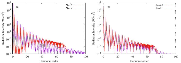
Figure 1: The HHG yield via logarithm of the radiation intensity $c\left|E^{(g)}\left(\omega\right)\right|^{2}/4\pi\$for the GNRs with low Fermi energy $\varepsilon_{F}=0.1\,\mathrm{eV}$ at the various widths $W=a_{0}N$, which define the single particle spectrum. (a) for $N=16$ (metallic) and $N=17$ (insulator) and (b) for larger widths: $N=40$ (metallic) and $N=41$ (insulator). We assume $\hbar\omega=0.041\,\mathrm{eV}$ ($\omega/(2\pi)=10\ \mathrm{THz}$). The pump wave intensity is taken to be $I_{0}=5.0\times 10^{8}\ \mathrm{W/cm}^{2}$.

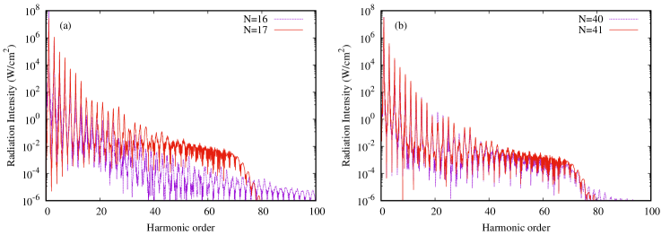
Figure 2: The same as for Fig. 1 but for large Fermi energy $\varepsilon_{F}=0.4\,\mathrm{eV}$.

In Fig. 2 we plot HHG spectra for relatively large Fermi energy $\varepsilon_{F}=0.4\,\mathrm{eV}$. In this case the situation is opposite. From Fig. 2(a) we see considerable enhancement of the HHG yield for the entire spectra for nonmetallic GNR. This is connected with the Pauli blocking. Thus, for large $\varepsilon_{F}>>\hbar\omega$ Pauli blocking reduces the probability of creation of electron-hole pairs in the case of gapless quasienergy spectrum. As in the case of Fig. 1(b) for relatively large widths the difference between both cases is minimal (see Fig. 2(b)).

We have also investigated the intensities of 3rd, 5th, 7th and 9th harmonics versus GNR width for Fermi energies $\varepsilon_{F}=0.1\,\mathrm{eV}$ and $\varepsilon_{F}=0.4\,\mathrm{eV}$. The latter is plotted in Fig. 3(a) and 3(b). For visual convenience we have rescaled the intensities. As is seen from Fig. 3(a), the intensities for the small Fermi energy are maximal in metallic GNRs ($N=13,16,19...$) up to $N=28$ harmonics. From Fig 3(b), we see that for the large Fermi energies overall the intensities are maximal in nonmetallic GNRs.

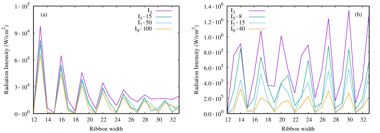
Figure 3: The intensities of 3rd, 5th, 7th and 9th harmonics versus nanoribbon width in units of $a_{0}$ ($N=W/a_{0}$). We assume $\omega/(2\pi)=10\ \mathrm{THz}$ and $I_{0}=5.0\times 10^{8}\ \mathrm{W/cm}^{2}$: (a) $\varepsilon_{F}=0.1\,\mathrm{eV}$ and (b) $\varepsilon_{F}=0.4\,\mathrm{eV}$.

As we see from Figs. 1 and 2, the high-order harmonics up to the 80th orders are appeared. Note that only odd harmonics are generated, reflecting the inversion symmetry preserved in the GNRs. One of the main questions at HHG is the cutoff harmonic dependence on the intensity of the pump wave. In Fig. 4, we plot the HHG yield for the GNR of width $W=17a_{0}$ for the various pump wave intensities at fixed frequency. As is seen, the cutoff harmonic is proportional to $I^{1/2}$.

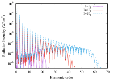
Figure 4: The HHG yield for the GNR of width $W=17a_{0}$ for various pump wave intensities at fixed frequency. We assume $\hbar\omega=0.041\,\mathrm{eV}$ ($\omega/(2\pi)=10\ \mathrm{THz}$), $I_{1}=3.5\times 10^{7}\ \mathrm{W/cm}^{2}$ and Fermi energy $\varepsilon_{F}=0.1\,\mathrm{eV}$.

In order to see the physical origin behind this dependence we will examine Eq. (11). Formally the solution of the latter can be written as

$$\mathcal{P}_{n}(k_{y},t)=\frac{ie}{\hbar}\int_{0}^{t}dt^{\prime}y_{\mathrm{tr}}\left(n,\widetilde{k}\left(t,t^{\prime}\right)\right)E\left(t^{\prime}\right)\left(N_{v,n}(\widetilde{k}\left(t,t^{\prime}\right),t^{\prime})-N_{c,n}(\widetilde{k}\left(t,t^{\prime}\right),t^{\prime})\right)$$

$$\times\exp\left(2i\mathrm{v}_{F}\int_{t^{\prime}}^{t}\sqrt{k_{n}^{2}+\widetilde{k}\left(t,t_{1}\right)}dt_{1}\right)\exp\left(-\Gamma_{n}\left(t-t^{\prime}\right)\right)$$ (18)

where

$$\widetilde{k}\left(t,t^{\prime}\right)=k_{y}+\frac{e}{\hbar}\int_{t^{\prime}}^{t}E\left(\tau\right)d\tau$$

is the classical momentum change in the wave field. The time dependence of $\mathcal{P}_{n}(k_{y},t)$ is mainly determined by the exponential factor with the electron-hole energy in the field $\ \varepsilon_{eh}\left(n,t,t^{\prime}\right)=2\mathrm{v}_{F}\hbar\sqrt{k_{n}^{2}+\widetilde{k}\left(t,t^{\prime}\right)}$. The cutoff frequency is determined by electron-hole pairs recolliding with the highest energy $\hbar\omega_{c}\sim\varepsilon_{eh}\left(n,t,t^{\prime}\right)_{\max}$. For the strong wave fields $\widetilde{k}_{\max}=2eE_{0}/\hbar\omega>>k_{n}$ this yields to the linear dependence of the cutoff frequency on the pump radiation field: $\hbar\omega_{c}\simeq 4\mathrm{v}_{F}eE_{0}/\omega$. This cutoff frequency is close to numerical values determined from Fig. 4.

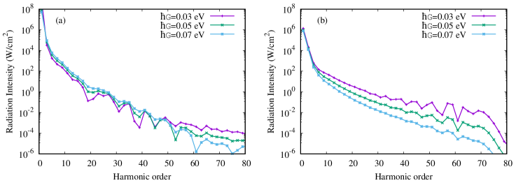
Figure 5: The HHG yield for the GNR for various relaxation rates. We assume $\omega/(2\pi)=10\ \mathrm{THz}$, $I_{0}=5.0\times 10^{8}\ \mathrm{W/cm}^{2}$, and $\varepsilon_{F}=0.1\,\mathrm{eV}$: (a) $N=W/a_{0}=16$ and (b) $N=17$.

We have also investigated the HHG yield at various relaxation rates ($\Gamma\equiv\Gamma_{n}$) for metallic ($N=16$) and for band insulator ($N=17$) GNRs. The latter is plotted in Fig. 5. For visual convenience in the logarithmic scale we have plotted the envelope of the intensities on $2s+1$ harmonics . In Fig. 5 we see the considerable difference of the HHG yield depending on the quasiparticle spectrum of GNR. Fig. 5(a) shows the robustness of HHG in metallic GNR against relaxation processes in contrast to a band insulator case demonstrated in Fig. 5(b), where harmonics are suppressed at high relaxation rates.

IV Conclusion

We have presented the microscopic theory of nonlinear interaction of the GNRs with a strong coherent radiation field. For the extreme nonlinear optical response, we have used a free quasiparticle model and obtained a closed set of differential equations for the single-particle density matrix with the phenomenological relaxation terms. These equations have been solved numerically. We have considered multiphoton excitation of GNRs towards the high-order harmonics generation. It has been shown that the width size and Fermi energy level of the GNR in the nonlinear optical response are quite considerable. For the low Fermi energies $\varepsilon_{F}\sim\hbar\omega$ we obtained a considerable enhancement of the HHG yield up to the middle of the spectra in metallic GNR compared with the nonmetallic ones. For the large Fermi energies $\varepsilon_{F}>>\hbar\omega$, the nonmetallic GNRs are more effective for HHG. We extracted the linear upon the pump field amplitude dependence on the HHG cutoff frequency. Obtained results show that GNRs can serve as an effective medium for the high-order harmonic generation with radiation fields of moderate intensities due to the confinement of quasiparticles in GNRs.

- (1) A. H. Castro Neto, F. Guinea, N. M. R. Peres, K. S. Novoselov, and A. K. Geim, “The electronic properties of graphene”, Rev. Mod. Phys. 81, 109-162 (2009).
- (2) S. A. Mikhailov, K. Ziegler, “Nonlinear EM response of graphene: frequency multiplication and the self-consistent-field effects”, J. Phys. Condens. Matter 20, 384204(1)–384204(10) (2008).
- (3) H. K. Avetissian, A. K. Avetissian, G. F. Mkrtchian, K. V. Sedrakian,“Multiphoton resonant excitation of Fermi-Dirac sea in graphene at the interaction with strong laser fields,”J. Nanophotonics 6, 061702(1)-061702(16). (2012)..
- (4) H. K. Avetissian, G. F. Mkrtchian, K. G. Batrakov, S. A. Maksimenko, A. Hoffmann, “Multiphoton resonant excitations and high-harmonic generation in bilayer grapheme”, Phys. Rev. B. 88, 165411(1)–165411(9) (2013).
- (5) I. Al-Naib, J. E. Sipe and M. M. Dignam, “Nonperturbative model of harmonic generation in undoped graphene in the terahertz regime”, New J. Phys. 17, 113018(1)–113018(17) (2015).
- (6) L. A. Chizhova, F. Libisch, J. Burgdorfer, “Nonlinear response of graphene to a few-cycle terahertz laser pulse: Role of doping and disorder”, Phys. Rev. B 94, 075412(1)–075412(10) (2016).
- (7) H. K. Avetissian, A.G. Ghazaryan, G. F. Mkrtchian, K. V. Sedrakian, “High harmonic generation in Landau-quantized graphene subjected to a strong EM radiation”, J. Nanophoton. 11, 016004(1)–016004(9) (2017).
- (8) L. A. Chizhova, F. Libisch, and J. Burgdorfer , “High-harmonic generation in graphene: Interband response and the harmonic cutoff”, Phys. Rev. B 95, 085436(1)– 085436(8) (2017).
- (9) D. Dimitrovski, L. B. Madsen, T. G. Pedersen, “High-order harmonic generation from gapped graphene”, Phys. Rev. B 95, 035405(1)–035405(9) (2017).
- (10) H. K. Avetissian, G.F. Mkrtchian, “Impact of electron-electron Coulomb interaction on the high harmonic generation process in graphene”, Phys. Rev. B 97, 115454(1)–115454(9) (2018).
- (11) H. K. Avetissian, A. K. Avetissian, B. R. Avchyan, G. F. Mkrtchian, “Wave mixing and high harmonic generation at two-color multiphoton excitation in two-dimensional hexagonal nanostructures”, Phys. Rev. B 100, 035434(1)–035434(8) (2019).
- (12) P. Bowlan, E. Martinez-Moreno, K. Reimann, T. Elsaesser, and M. Woerner, “Ultrafast terahertz response of multilayer graphene in the nonperturbative regime”, Phys. Rev. B 89, 041408(1)–041408(5) (2014).
- (13) N. Yoshikawa, T. Tamaya, K. Tanaka, “High-harmonic generation in graphene enhanced by elliptically polarized light excitation”, Science 356, 736–738 (2017).
- (14) H. K. Avetissian, A. K. Avetissian, G. F. Mkrtchian, K. V. Sedrakian, “Creation of particle-hole superposition states in graphene at multiphoton resonant excitation by laser radiation”, Phys. Rev. B 85, 115443(1)–115443(10) (2012).
- (15) A. K. Avetissian, A.G. Ghazaryan, K. V. Sedrakian, and B. R. Avchyan, “Microscopic nonlinear quantum theory of absorption of strong EM radiation in doped graphene”, J. Nanophoton. 12, 016006(1)–016006(12) (2018).
- (16) M.Y. Han, B. Özyilmaz, Y. Zhang, and P. Kim, “Energy band-gap engineering of graphene nanoribbons”, Phys. Rev. Lett. 98, 206805(1)- 206805(4) (2007).
- (17) L. Brey and H. A. Fertig, “Electronic states of graphene nanoribbons studied with the Dirac equation”, Phys. Rev. B 73, 235411(1)-235411(5) (2006).
- (18) L. Yang, M. L. Cohen, S. G. Louie, “Excitonic effects in the optical spectra of graphene nanoribbons”, Nano Lett. 7, 3112–3115 (2007).
- (19) D. Prezzi, D. Varsano, A. Ruini, A. Marini, E. Molinari, “Optical properties of graphene nanoribbons: the role of many-body effects”, Phys. Rev. B 77, 041404(1)-041404(4) (2008).
- (20) D. Prezzi, D. Varsano, A. Ruini, E. Molinari, “Quantum dot states and optical excitations of edge-modulated graphene nanoribbons”, Phys. Rev. B 84, 041401(1)-041401(4) (2011).
- (21) E. H. Hwang and S. Das Sarma, “Dielectric function, screening, and plasmons in two-dimensional graphene”, Phys. Rev. B 75, 205418(1)-205418(6) (2007).
- (22) F. H. Koppens, D. E. Chang, and F. J. Garcia de Abajo, “Graphene plasmonics: a platform for strong light–matter interactions”, Nano letters 11, 3370-3377 (2011).
- (23) S. A. Mikhailov, “Theory of the giant plasmon-enhanced second-harmonic generation in graphene and semiconductor two-dimensional electron systems”, Phys. Rev. B 84, 045432(1)- 045432(6) (2011).
- (24) M. Gullans, D. E. Chang, F. H. L. Koppens, F. J. Garcia de Abajo, and M. D. Lukin, “Single-Photon Nonlinear Optics with Graphene Plasmons”, Phys. Rev. Lett. 111, 247401(1)-247401(4) (2013).
- (25) V. W. Brar, M. S. Jang, M. Sherrott, J. J. Lopez, and H. A. Atwater, “Highly Confined Tunable Mid-Infrared Plasmonics in Graphene Nanoresonators”, Nano Lett. 13, 2541-2547 (2013).
- (26) T. J. Constant, S. M. Hornett, D. E. Chang, and E. Hendry, “All-Optical Generation of Surface Plasmons in Graphene”, Nature Physics 12, 124-127 (2016).
- (27) V. V. Popov, T. Yu. Bagaeva, T. Otsuji, and V. Ryzhii, “Oblique terahertz plasmons in graphene nanoribbon arrays”, Phys. Rev. B 81, 073404(1)-073404(4) (2010).
- (28) M. Lewenstein, Ph. Balcou, Ivanov M Yu, A. L’Huillier, and P. B. Corkum, “Theory of high-harmonic generation by low-frequency laser fields”, Phys. Rev. A 49 2117–2132 (1994).
- (29) R. Binder, D. Scott, A. E. Paul, M. Lindberg, K. Henneberger, and S. W. Koch, “Carrier-carrier scattering and optical dephasing in highly excited semiconductors”, Phys. Rev. B 45, 1107- 1115 (1992).
- (30) E. Malic, T. Winzer, E. Bobkin, and A. Knorr, “Microscopic theory of absorption and ultrafast many-particle kinetics in graphene”, Phys. Rev. B 84, 205406(1)- 045432(17) (2011).