High laser harmonics induced by the Berry curvature in time-reversal invariant materials

Abstract

A new nonlinear scheme of high harmonics generation in a wide class of time-reversal invariant materials with broken spatial inversion symmetry (where recently the nonlinear Hall effect has been established) due to the nontrivial topology of bands is proposed. A microscopic quasiclassical theory describing the nonperturbative optical response of pseudo-relativistic electrons with nonzero Berry curvature of bands to a strong laser field is developed. We analyze the harmonic content of the induced current and show that one can decouple induced laser harmonics solely by the Berry curvature of bands. We also study the dependence of the nonlinear response on the driving wave and system parameters.

I Introduction

According to Landau’s Fermi-liquid theory,Landau9 the charge transport in metals involves only quasiparticles with energies near the Fermi level and depends on bandstructure property at the Fermi level. This is true for bands with trivial topology. However, for the bands with nontrivial topology, there is an “anomalous velocity”Kar-Lut  of Bloch electrons which can be represented in terms of the Berry curvatureBerry ; Xiao2010 of occupied electronic Bloch states.Sundaram ; Jungwirth ; Haldane At that, the Berry curvature acts as an effective magnetic field in momentum space.

The Berry curvature being a local gauge field of topological nature depends on the space-time symmetries of the material. It vanishes in materials that are symmetric with respect to both spatial and time inversions. In materials with broken time-reversal symmetry, the Berry curvature leads to an anomalous Hall effect.AHE ; Qian There is a wide class of materials with non-zero Berry curvature in which the spatial inversion symmetry is broken but the time-reversal is preserved. These are topological insulators,Hasan transition metal dichalcogenides,Xiao ; Mak ; Lensky gapped monolayer and bilayer graphene systems,Gorbachev ; Sui as well as band-gap modified black phosphorus.Li ; Rodin ; Low In graphenelike systems the Dirac cones always appear in pairs ($K$, $-K$),Witten and if the spatial inversion symmetry is broken the Dirac cones become massive acquiring nonzero Berry curvatures of opposite signs. The latter is the result of time-reversal symmetry. In contrast to graphenelike systems in monolayer black phosphorus the conduction and valence band edges are located at the $\Gamma$ point of the rectangular Brillouin zone.Low

In the linear response regime, the net topological current identically vanishes because of time-reversal symmetry.Ashcroft Recently, it has been shown that in the nonlinear response regime, the topological current is not subject to such symmetry constraints.Sod-Fu Two recent experiments have independently observed second order nonlinear Hall effect in bilayerMa and multi-layer WTe₂.Kang

The mentioned novel materials with broken inversion symmetry are intensively considered as an effective medium for the high-order wave mixing and high harmonic generation (HHG). In particular, HHG has been considered in gapped graphenegg and bilayer graphene systems,bgg ; Ikeda in monolayers of black phosphorus,bf transition metal dichalcogenides,TMD1 ; TMD2 ; 2020 hexagonal boron nitride,HBN and in buckled two-dimensional hexagonal nanostructures.2019a ; 2019b

In the last few years, there is a growing interest to use the electronic response of materials to strong fields for retrieving the electronic properties of novel nanostructures.Kruchinin ; Schotz At that the HHG being the hallmark of strong-field physics plays the central role. The HHG in solids originates either from the intraband electronic current or from the interband transitions. In both processes, the topology of bands has a considerable impact. In particular, Berry curvature affects the excitonic spectrum in transition metal dichalcogenides along with dynamic energy modulation due to the Berry connection of bands and consequently has a sizeable impact on the nonlinear response.2020 ; mks2019 The field-driven injection of electrons across the bandgap strongly depends on the Berry curvature which defines the structure and timing of HHG spectra.Silva The topology of bands can also result in distinct by orders strong-field HHG spectra.Bauer ; Drueke More interestingly, the polarization resolved HHG spectra allowed to measure the Berry curvature of $\alpha$-quartz.Luu

When both interband and intraband mechanisms act simultaneously the sole contribution of Berry curvature in the nonlinear response is difficult to separate in materials with time-reversal symmetry. In the highly doped systems, one can exclude interband transitions and also effectively screen the many-body Coulomb effects opening the way for the manifestation of nonlinear topological effects. In this case, only states close to the Fermi surface will contribute to HHG processes in the low-temperature limit, so that this response will be a Fermi liquid property as in case of second-order nonlinear Hall effect.Sod-Fu Hence, it is of actual interest to study the mentioned graphenelike nanostructures physics in the presence of intense optical fields that can lead to the effective generation of high harmonics by the Berry curvature of bands.

In the present work, we develop a quasiclassical theory describing the nonperturbative optical response of pseudo-relativistic electrons with nonzero Berry curvature of bands to a strong laser field. As a model time-reversal invariant system we consider massive Dirac nanostructure where the Dirac cones are tilted.

The paper is organized as follows. In Sec. II the theoretical model and near-analytical expression for the topological current including contributions from all orders in the field are presented. In Sec. III, we examine the harmonic content of the induced current depending on the system and pump wave parameters. Finally, conclusions are given in Sec. IV.

II THEORETICAL MODEL   

The spectacular transport properties of Dirac materials are connected with the spinor nature of their electronic wavefunctions and linear dispersion law around the Dirac points. As was mentioned, the Dirac cones (in graphenelike systems) always appear in pairs ($K$, $-K$). The nonlinear topological current is characterized by the odd order moments of Berry curvatures over occupied states. The second-order nonlinear topological current is characterized by the first order moment of Berry curvature, called the Berry curvature dipole. The latter is proposed to exist in transition metal dichalcogenides,You ; Zhang ; Zhou time-reversal symmetric Weyl semimetals,Sod-Fu in the giant Rashba material BiTeI,Facio as well as in the strained graphene.Battilomo In addition to inversion symmetry breaking the common feature of all these materials is the breaking of the three-fold ($C_{3}$) symmetry. The latter results either low-energy Dirac quasi-particles forming tilted Dirac cones or trigonal warping of the Fermi surface. In the present paper we will consider strained nanostructure with tilted Dirac cones. The application of strain to the lattice deforms the corresponding Brillouin zone, and the Fermi velocity also becomes anisotropic. The low energy model Hamiltonian up to the first order in quasimomentum $p$ (relative to $\tau K$ points) will be:

$$\widehat{H}_{0}=\begin{bmatrix}\Delta+\tau\alpha p_{x}&\tau\mathrm{v}_{x}p_{x}-i\mathrm{v}_{y}p_{y}\\ \tau\mathrm{v}_{x}p_{x}+i\mathrm{v}_{y}p_{y}&-\Delta+\tau\alpha p_{x}\end{bmatrix},$$ (1)

where $\tau=\pm 1$ is the valley index, $\mathrm{v}_{x}$ and $\mathrm{v}_{y}$ are Fermi velocities, $2\Delta$ is the gap. The term $\alpha$ produces a finite tilt in the Dirac cones. This tilting effect is allowed by symmetry and it is crucial to get a nonvanishing net topological current. The eigenenergies of the Hamiltonian (1) for valence ($v$) and conduction ($c$) bands are $\mathcal{E}_{v\tau}\left(\mathbf{p}\right)=\alpha\tau p_{x}-\mathcal{E}$ and $\mathcal{E}_{c\tau}\left(\mathbf{p}\right)=\alpha\tau p_{x}+\mathcal{E}$, with $\mathcal{E=}\sqrt{\Delta^{2}+\mathrm{v}_{x}^{2}p_{x}^{2}+\mathrm{v}_{y}^{2}p_{y}^{2}}$.

We consider the interaction of a strong wave field $\mathbf{E}(t)$ with the nanostructure. The wave propagates in a perpendicular direction to the nanostructure plane ($XY$):

$$\mathbf{E}\left(t\right)=f\left(t\right)E_{0}\hat{\mathbf{e}}\cos\omega t,$$ (2)

with the frequency $\omega$, polarization $\hat{\mathbf{e}}$ unit vector, pulse duration $\mathcal{T}=40\pi/\omega$, and envelope $f\left(t\right)=\sin^{2}\left(\pi t/\mathcal{T}\right)$.

We will consider a highly electron-doped system and we will neglect excitonic effects since free carriers introduced through doping will effectively screen the Coulomb interaction. Thus, the dynamics of charge carriers is described by a single-particle density matrix. We use the second quantization formalism, expanding the fermionic field operators on the basis eigenstates of a single particle Hamiltonian (1): $\hat{\Psi}(\mathbf{r})=\sum_{\lambda,\mathbf{k}}\hat{e}_{\lambda\mathbf{k}}|\lambda;\mathbf{k}\rangle e^{i\mathbf{kr}},$ where $\hat{e}_{\lambda\mathbf{k}}$ ($\hat{e}_{\lambda\mathbf{k}}^{\dagger}$) are the annihilation (creation) operators for an electron with momentum $\mathbf{k}$, and $\lambda=\left\{b,\tau\right\}$ the set of quantum numbers (band and valley). The total Hamiltonian in the second quantization reads:

$$\hat{H}=\hat{H}_{\mathrm{free}}+\hat{H}_{\mathrm{int}},$$ (3)

where

$$\hat{H}_{\mathrm{\ free}}=\sum_{\tau,\mathbf{p}}\left(\mathcal{E}_{c\tau}\left(\mathbf{p}\right)\hat{e}_{c\tau\mathbf{p}}^{\dagger}\hat{e}_{c\tau\mathbf{p}}+\mathcal{E}_{v\tau}\left(\mathbf{p}\right)\hat{e}_{v\tau\mathbf{p}}^{\dagger}\hat{e}_{v\tau\mathbf{p}}\right)$$ (4)

is the free particle Hamiltonian, and

$$\hat{H}_{\mathrm{int}}=e\mathbf{E}(t)\cdot\widehat{\mathbf{r}}$$ (5)

is the light-matter interaction Hamiltonian, with the elementary charge $e$ and position operator in the second quantization: $\widehat{\mathbf{r}}=\widehat{\mathbf{r}}_{i}+\widehat{\mathbf{r}}_{\mathrm{B}}+\widehat{\mathbf{r}}_{e}$. Here

$$\widehat{\mathbf{r}}_{i}=i\hbar\sum\limits_{\tau,\mathbf{p,p}^{\prime}}\delta_{\mathbf{p}^{\prime}\mathbf{p}}\partial_{\mathbf{p}^{\prime}}\left(\hat{e}_{c\tau\mathbf{p}}^{\dagger}\hat{e}_{c\tau\mathbf{p}^{\prime}}+\hat{e}_{v\tau\mathbf{p}}^{\dagger}\hat{e}_{v\tau\mathbf{p}^{\prime}}\right)$$ (6)

is the intraband part of position operator and

$$\widehat{\mathbf{r}}_{\mathrm{B}}=\sum\limits_{\tau,\mathbf{p}}\mathbf{A}_{\tau}\left(\mathbf{p}\right)\left(\widehat{e}_{c\tau\mathbf{p}}^{+}\widehat{e}_{c\tau\mathbf{p}}-\widehat{e}_{v\tau\mathbf{p}}^{+}\widehat{e}_{v\tau\mathbf{p}}\right)$$ (7)

is defined by the topology of bands with the Berry connection:

$$\mathbf{A}_{\tau}\left(\mathbf{p}\right)=\hbar\langle b\tau\mathbf{p}|i\partial_{\mathbf{p}}|b\tau\mathbf{p}\rangle.$$ (8)

The last term

$$\widehat{\mathbf{r}}_{e}=\sum\limits_{\tau,\mathbf{p}}\left(\mathbf{D}_{\mathrm{tr}}\left(\tau;\mathbf{p}\right)\widehat{e}_{v\tau\mathbf{p}}^{+}\widehat{e}_{c\tau\mathbf{p}}+\mathrm{h.c.}\right)$$

defines interband current with the transition dipole moment $\mathbf{D}_{\mathrm{tr}}\left(\tau,\mathbf{p}\right)=e\hbar\langle v\tau\mathbf{p}|i\partial_{\mathbf{p}}|c\tau\mathbf{p}\rangle$. To separate the topological part of interaction we will consider the electron-doped system neglecting interband transitions. The conditions which justify this will be presented further. Thus, we can consider only conduction band dynamics with the total Hamiltonian

$$\hat{H}^{\prime}=\sum_{\tau,\mathbf{p}}\mathcal{E}_{c\tau}\left(\mathbf{p}\right)\hat{e}_{c\tau\mathbf{p}}^{\dagger}\hat{e}_{c\tau\mathbf{p}}+e\mathbf{E}(t)i\hbar\sum\limits_{\tau,\mathbf{p,p}^{\prime}}\delta_{\mathbf{p}^{\prime}\mathbf{p}}\partial_{\mathbf{p}^{\prime}}\hat{e}_{c\tau\mathbf{p}}^{\dagger}\hat{e}_{c\tau\mathbf{p}^{\prime}}$$

$$+e\mathbf{E}(t)\sum\limits_{\tau,\mathbf{p}}\mathbf{A}_{\tau}\left(\mathbf{p}\right)\widehat{e}_{c\tau\mathbf{p}}^{+}\widehat{e}_{c\tau\mathbf{p}}.$$ (9)

The response of the system to electromagnetic wave is determined by the intraband current density $\mathbf{j}=-e\left\langle d\widehat{\mathbf{r}}/dt\right\rangle$, which from Heisenberg equation can be written as

$$\mathbf{j}=-e\frac{1}{i\hbar}\left\langle\left[\widehat{\mathbf{r}}_{i}+\widehat{\mathbf{r}}_{\mathrm{B}},\widehat{H}^{\prime}\right]\right\rangle.$$ (10)

Taking into account fermion anticommutator rules, with the help of Eqs. (6), (7), and (9) from Eq. (10) one can obtain the intraband surface current

$$\mathbf{j}\left(t\right)=-eg\sum_{\mathbf{p}\tau}\left(\mathbf{V}_{\tau}\left(\mathbf{p}\right)+\frac{e}{\hbar}\left[\mathbf{E}(t)\times\mathbf{B}_{\tau}\left(\mathbf{p}\right)\right]\right)\mathcal{N}_{c\tau}\left(\mathbf{p},t\right),$$ (11)

where $\mathbf{V}_{\tau}\left(\mathbf{p}\right)=\partial\mathcal{E}_{c\tau}\left(\mathbf{p}\right)/\partial\mathbf{p}$ is the velocity of band,

$$\mathbf{B}_{\tau}\left(\mathbf{p}\right)=\hbar\mathrm{rot}_{\mathbf{p}}\left(\mathbf{A}_{\tau}\left(\mathbf{p}\right)\right)$$ (12)

is the Berry curvature, $\mathcal{N}_{c\tau}\left(\mathbf{p},t\right)=\langle\hat{e}_{c\tau\mathbf{p}}^{\dagger}\left(t\right)\hat{e}_{c\tau\mathbf{p}}\left(t\right)\rangle$ is the distribution function of electrons, and $g$ is the degeneracy factor. The second term in Eq. (11) is an “anomalous current” Kar-Lut  represented in terms of the Berry curvature. From Heisenberg equation $i\hbar\partial\hat{e}_{c\tau\mathbf{p}}^{\dagger}\hat{e}_{c\tau\mathbf{p}}/\partial t=\left[\hat{e}_{c\tau\mathbf{p}}^{\dagger}\hat{e}_{c\tau\mathbf{p}},\widehat{H}^{\prime}\right]$ one can also obtain evolutionary equations for $\mathcal{N}_{c\tau}\left(\mathbf{p},t\right)$. In addition we will assume that the system relaxes at a rate $\gamma$ to the equilibrium $\mathcal{N}_{c\tau}^{(0)}\left(\mathbf{p}\right)$ distribution. Thus, we obtain the Boltzmann equation for the distribution of electrons

$$\frac{\partial\mathcal{N}_{c\tau}\left(\mathbf{p},t\right)}{\partial t}-e\mathbf{E}\left(t\right)\frac{\partial\mathcal{N}_{c\tau}\left(\mathbf{p},t\right)}{\partial\mathbf{p}}=-\gamma\left(\mathcal{N}_{c\tau}\left(\mathbf{p},t\right)-\mathcal{N}_{c\tau}^{(0)}\left(\mathbf{p}\right)\right).$$ (13)

We construct $\mathcal{N}_{c\tau}^{(0)}$ from the filling of electron states according to the Fermi–Dirac-distribution $f_{FD}$:

$$\mathcal{N}_{c\tau}^{(0)}\left(\mathbf{p}\right)=f_{FD}\left(\mathcal{E}_{c\tau}\left(\mathbf{p}\right)\right)=\frac{1}{1+\exp\left(\frac{\mathcal{E}_{c\tau}\left(\mathbf{p}\right)-\varepsilon_{F}}{T}\right)}.$$ (14)

Here $\varepsilon_{F}$ is the Fermi energy and $T$ is the temperature in energy units. Note that this relaxation approximation provides an accurate description for optical field components oscillating at frequencies $\omega>>\gamma$.

The differential equation (13) can be solved exactly by the method of characteristics, which yieldsPeres

$$\mathcal{N}_{c\tau}\left(\mathbf{p},t\right)=\gamma\int\nolimits_{-\infty}^{t}dt^{\prime}e^{-\gamma\left(t-t^{\prime}\right)}\mathcal{N}_{c\tau}^{(0)}(\mathbf{p+p}_{E}\left(t,t^{\prime}\right)),$$ (15)

where

$$\mathbf{p}_{E}\left(t,t^{\prime}\right)=e\int\nolimits_{t^{\prime}}^{t}\mathbf{E}\left(t^{\prime\prime}\right)dt^{\prime\prime}.$$ (16)

is the momentum given by the wave field.

We will consider the case of a low frequency driving wave $2\varepsilon_{F}/\hbar\omega>>1$. It is clear, that a strong field will induce multiphoton ($n_{0}>2\varepsilon_{F}/\hbar\omega>>1$) and/or tunneling transitions from the valence to the conduction band. To neglect the interband transitions one should restrict the field strength. When a gapped sample is exposed to an intense laser field the interband transition mechanisms are distinguished by the KeldyshKeldysh64 parameter $\gamma_{K}=\delta_{t}\omega$, where $\delta_{t}$ is the tunneling time. In considered case the tunneling time is determined by the mean time of the electron passing through a barrier of width $2\varepsilon_{F}/eE_{0}$ with the velocity $\mathrm{v}_{x}$. Thus, the Keldysh parameter will be

$$\gamma_{K}=\frac{2\varepsilon_{F}\omega}{eE_{0}\mathrm{v}_{x}}.$$ (17)

At the satisfaction of the condition $2\varepsilon_{F}/\hbar\omega>>1$ in the strong fields when $\gamma_{K}<<1$, the interband transitions take place via the tunneling. Thus, we will consider the so-called nonadiabatic regime $\gamma_{K}\gtrsim 1$ when tunneling is suppressed and the probabilities of multiphoton transitions are negligible since $n_{0}>>1$. This is a quasiclassical regime when the wave-particle interaction can be characterized by the amplitude of the energy $eE_{0}\mathrm{v}_{x}/\omega$ of an electron oscillatory motion in the wavefield. The condition $\gamma_{K}>1$ can be written as

$$\frac{eE_{0}\mathrm{v}_{x}}{\omega}<2\varepsilon_{F}.$$ (18)

This means that the wavefield can not provide a sufficient energy for the creation of an electron-hole pair.

With the help of the solution (15) the topological part of the induced current can be represented as

$$\mathbf{j}_{\mathrm{T}}\left(t\right)=-\frac{e^{2}\gamma g}{4\pi^{2}\hbar^{3}}\sum_{\tau}\int\nolimits_{-\infty}^{t}dt^{\prime}\int d\mathbf{p}\left(\mathbf{E}(t)\times\mathbf{B}_{\tau}\left(\mathbf{p}\right)\right)$$

$$\times e^{-\gamma\left(t-t^{\prime}\right)}\mathcal{N}_{c\tau}^{(0)}(\mathbf{p+\mathbf{p}}_{E}\left(t,t^{\prime}\right)\mathbf{).}$$ (19)

Taking into account the time reversal symmetry: $\mathcal{N}_{c\tau}^{(0)}\left(\mathbf{p}\right)=\mathcal{N}_{c-\tau}^{(0)}\left(-\mathbf{p}\right)$ and $\mathbf{B}_{\tau}\left(\mathbf{p}\right)=-\mathbf{B}_{-\tau}\left(-\mathbf{p}\right)$ the $\mathbf{j}_{\mathrm{T}}$ can be expressed as

$$\mathbf{j}_{\mathrm{T}}\left(t\right)=-\frac{e^{2}\gamma g}{4\pi^{2}\hbar^{2}}\int d\mathbf{p}\int\nolimits_{-\infty}^{t}dt^{\prime}e^{-\gamma\left(t-t^{\prime}\right)}\mathcal{N}_{c1}^{(0)}(\mathbf{p})$$

$$\times\left[\mathbf{E}(t)\times\left(\mathbf{B}_{1}\left(\mathbf{p-p}_{E}\left(t,t^{\prime}\right)\right)-\mathbf{B}_{1}\left(\mathbf{p+p}_{E}\left(t,t^{\prime}\right)\right)\right)\right].$$ (20)

This result provides a near-analytical expression for the topological current including contributions from all orders in the field. When $\mathbf{E}\left(t\right)=0$, $\mathbf{j}_{\mathrm{T}}=0$. Since $\mathbf{B}\left(\mathbf{p}\right)=\mathbf{B}\left(-\mathbf{p}\right)$, when a tilt is absent $\alpha=0$, then $\mathcal{N}_{c1}^{(0)}(\mathbf{p})=\mathcal{N}_{c1}^{(0)}\left(-\mathbf{p}\right)$, and $\mathbf{j}_{\mathrm{T}}=0$. The net topological current is vanishing also when the field is perpendicular to tilt direction. From the dependence on the field $\mathbf{j}_{\mathrm{T}}\left(\mathbf{E}\right)=\mathbf{j}_{\mathrm{T}}\left(-\mathbf{E}\right)$ it is apparent that the topological current contains only even orders of nonlinear response and is directed perpendicular to the pump field. As is seen the topological current strongly depends on tilt parameter $\alpha$. The leading order $\sim\alpha$ of which can be obtained from Eq. (20) by expanding Fermi–Dirac-distribution function:

$$\mathbf{j}_{\mathrm{T}}\left(t\right)\simeq\alpha\frac{e^{2}\gamma g}{2\pi^{2}\hbar^{2}}\int d\mathbf{p}\int\nolimits_{-\infty}^{t}dt^{\prime}e^{-\gamma\left(t-t^{\prime}\right)}p_{x}\frac{\partial f_{FD}\left(\mathcal{E}\right)}{\partial\mathcal{E}}$$

$$\times\left[\mathbf{E}(t)\times\mathbf{B}_{1}\left(\mathbf{p+p}_{E}\left(t,t^{\prime}\right)\right)\right].$$ (21)

The regular part of the current can be represented as

$$\mathbf{j}_{\mathrm{r}}\left(t\right)=-\frac{e\gamma g}{4\pi^{2}\hbar^{2}}\sum_{\tau}\int\nolimits_{-\infty}^{t}dt^{\prime}e^{-\gamma\left(t-t^{\prime}\right)}$$

$$\times\int d\mathbf{pV}_{\tau}\left(\mathbf{p-p}_{E}\left(t,t^{\prime}\right)\right)\mathcal{N}_{c\tau}^{(0)}\left(\mathbf{p}\right).$$ (22)

Taking into account the time reversal symmetry $\mathbf{V}_{1}\left(\mathbf{p}\right)=\mathbf{V}_{-1}\left(-\mathbf{p}\right)$ it can be expressed as

$$\mathbf{j}_{\mathrm{r}}\left(t\right)=-\frac{e\gamma g}{4\pi^{2}\hbar^{2}}\int\nolimits_{-\infty}^{t}dt^{\prime}e^{-\gamma\left(t-t^{\prime}\right)}\int d\mathbf{p}$$

$$\times\left[\mathbf{V}_{1}\left(\mathbf{p-p}_{E}\left(t,t^{\prime}\right)\right)-\mathbf{V}_{1}\left(\mathbf{p+p}_{E}\left(t,t^{\prime}\right)\right)\right]\mathcal{N}_{c1}^{(0)}(\mathbf{p}).$$ (23)

From Eq. (23) it is clear that $\mathbf{j}_{\mathrm{r}}\left(\mathbf{E}\right)=-\mathbf{j}_{\mathrm{r}}\left(-\mathbf{E}\right)$. The regular current contains only odd orders of nonlinear response and is directed along the pump field. When a tilt is absent $\alpha=0$, then $\mathcal{N}_{c1}^{(0)}(\mathbf{p})=\mathcal{N}_{c1}^{(0)}\left(-\mathbf{p}\right)$ and the regular current can be written as:

$$\mathbf{j}_{\mathrm{r}}\left(t\right)=-\frac{e\gamma g}{2\pi^{2}\hbar^{2}}\int\nolimits_{-\infty}^{t}dt^{\prime}e^{-\gamma\left(t-t^{\prime}\right)}\int d\mathbf{pV}_{1}\left(\mathbf{p-p}_{E}\left(t,t^{\prime}\right)\right)\mathcal{N}_{c1}^{(0)}(\mathbf{p}).$$ (24)

The last formula represents total interband current when three-fold ($C_{3}$) symmetry is preserved. On the base of Eq. (24) in the nonperturbative regime with corresponding velocity $\mathbf{V}_{1}\left(\mathbf{p}\right)$ dependence on $\mathbf{p}$ the HHG processes have been investigated in grapheneMikhailov and in monolayer black phosphorus.bf

To proceed it is also useful to present multipole expansion of the topological current (20). For concreteness we will consider x-polarized wave $\widehat{\mathbf{e}}=\widehat{\mathbf{x}}$ and utilize the Taylor expansion of the Berry curvature in Eq. (20)

$$B_{1z}\left(p_{x}+p_{E},p_{y}\right)=\sum\limits_{n=0}^{\infty}\frac{\partial^{n}B_{1z}\left(p_{x},p_{y}\right)}{\partial p_{x}^{n}}\frac{p_{E}^{n}}{n!}.$$

Taking into account that only odd orders of $p_{E}^{n}$ make contribution we obtain multipole expansion of the topological current

$$j_{y\mathrm{T}}\left(t\right)=-2e^{2}\gamma\sum\limits_{n=1}^{\infty}\frac{D_{x}^{\left(2n-1\right)}}{\left(2n-1\right)!}\int\nolimits_{-\infty}^{t}dt^{\prime}e^{-\gamma\left(t-t^{\prime}\right)}E_{x}(t)p_{E}^{2n-1}\left(t,t^{\prime}\right),$$ (25)

where

$$D_{x}^{\left(2n-1\right)}=g\int\frac{d\mathbf{p}}{\left(2\pi\hbar\right)^{2}}\mathcal{N}_{c1}^{(0)}(\mathbf{p})\frac{\partial^{2n-1}B_{1z}\left(p_{x},p_{y}\right)}{\partial p_{x}^{2n-1}}$$ (26)

is the $\left(2n-1\right)$-th moment of the Berry curvature in the momentum space. As is expected, in the leading order topological current is defined by the dipole moment of the Berry curvature. This corresponds to second order nonlinear Hall current derived by Sodemann and Fu.Sod-Fu The next nonvanishing moment is the octupole moment. From Eq. (25) it is easy to extract low-field perturbative limit of the topological current when $\left|p_{E}\right|<<p_{F}$ ($p_{F}$ is the Fermi momentum). At $\gamma<<\omega$ and for continuos wave we obtain perturbative limit of the topological current

$$j_{y\mathrm{T}}\left(t\right)=\sum\limits_{n=1}^{\infty}j_{y}^{(2n\omega)}\left(t\right),$$

where

$$j_{y}^{(2n\omega)}\left(t\right)=\frac{e^{2n+1}D_{x}^{\left(2n-1\right)}E_{0}^{2n}}{\omega^{2n-1}2^{2n-2}\left(2n-1\right)!}\sin 2n\omega t.$$ (27)

As is seen, in the perturbative limit the $\left(2n\right)$-th harmonic is defined by the $\left(2n-1\right)$-th moment of the Berry curvature. Note that for strong fields the current corresponding to $\left(2n\right)$-th harmonic may have sizable contribution from higher moments.

III Results

We further examine the nonlinear response of a nanostructure considering the generation of harmonics at the multiphoton excitation. We will consider low-temperature limit $T<<\varepsilon_{F}$. In this case the main contribution in the integrals determining topological (20) and regular (23) currents is made by the Fermi surface. We aim to keep the consideration rather generic introducing a limited number of dimensionless parameters. From Eqs. (8) and (12) one can calculate the Berry curvature

$$\mathbf{B}_{\tau}\left(\mathbf{p}\right)=-\frac{\Delta}{2}\tau\widehat{\mathbf{z}}\hbar^{2}\frac{\mathrm{v}_{x}\mathrm{v}_{y}}{\left(\Delta^{2}+\mathrm{v}_{x}^{2}p_{x}^{2}+\mathrm{v}_{y}^{2}p_{y}^{2}\right)^{3/2}}.$$ (28)

The band velocity $V_{x\tau}\left(\mathbf{p}\right)=\partial\mathcal{E}_{c\tau}\left(\mathbf{p}\right)/\partial p_{x}$ can also be calculated, which gives

$$V_{x\tau}\left(\mathbf{p}\right)=\alpha\tau+\frac{\mathrm{v}_{x}^{2}p_{x}}{\left(\Delta^{2}+\mathrm{v}_{x}^{2}p_{x}^{2}+\mathrm{v}_{y}^{2}p_{y}^{2}\right)^{1/2}}.$$ (29)

As is seen from Eq. (28) the tilting effect does not change the Berry curvature of the system but it is crucial to get a corresponding nonvanishing net topological current. The latter is determined by the odd-order moments of the Berry curvature in the momentum space (26). That is, one needs shear or warping of the Fermi surface: $N_{c\tau}^{(0)}(\mathbf{p})\neq N_{c\tau}^{(0)}\left(-\mathbf{p}\right)$. In considered case this is satisfied, since the Fermi surface is

$$\alpha\tau p_{x}+\sqrt{\Delta^{2}+\mathrm{v}_{x}^{2}p_{x}^{2}+\mathrm{v}_{y}^{2}p_{y}^{2}}=\varepsilon_{F}.$$ (30)

Making transformation $p_{y}\rightarrow\mathrm{v}_{x}/\mathrm{v}_{y}p_{y}$ one can see that the Fermi surface is an ellipse in the new coordinates (we assume that $\varepsilon_{F}>\Delta$). At $\alpha=0$ Fermi surface is a circle with Fermi momentum $p_{F}=\sqrt{\varepsilon_{F}^{2}-\Delta^{2}}/\mathrm{v}_{x}$. In Eq. (20) for integration we normalize $\mathbf{p}$ by the Fermi momentum and write $\overline{p}_{x}=p_{x}/p_{F}$, $\overline{p}_{y}\rightarrow\mathrm{v}_{y}/\mathrm{v}_{x}p_{y}/p_{F}$, $\overline{p}_{E}=p_{xE}/p_{F}$, and $\overline{\Delta}=\Delta/\left(\mathrm{v}_{x}p_{F}\right)$ so that

$$j_{y\mathrm{T}}\left(t\right)=\frac{e^{2}g}{4\pi^{2}\hbar}E_{x}(t)\frac{\overline{\Delta}}{2}\gamma\int\nolimits_{-\infty}^{t}dt^{\prime}e^{-\gamma\left(t-t^{\prime}\right)}\int d\overline{p}_{x}d\overline{p}_{y}$$

$$\times\frac{\mathcal{N}_{c1}^{(0)}(\overline{\mathbf{p}})-\mathcal{N}_{c-1}^{(0)}(\overline{\mathbf{p}})}{\left(\overline{\Delta}^{2}+\left(\overline{p}_{x}+\overline{p}_{E}\left(t,t^{\prime}\right)\right)^{2}+\overline{p}_{y}^{2}\right)^{3/2}},$$ (31)

where

$$\overline{p}_{E}\left(t,t^{\prime}\right)=\frac{F_{0}}{\sqrt{1-\frac{\Delta^{2}}{\varepsilon_{F}^{2}}}}\int\nolimits_{t^{\prime}}^{t}f\left(t^{\prime\prime}\right)\cos\left(\omega t^{\prime\prime}\right)d\left(\omega t^{\prime\prime}\right).$$ (32)

The dimensionless interaction parameter is defined as $F_{0}=eE_{0}\mathrm{v}_{x}/\left(\omega\varepsilon_{F}\right)$.   The interaction parameter $F_{0}$ is subject to the constraint (18), which yields $F_{0}<2$. Overall the topological current is defined by the following parameters: $F_{0}$, $\Delta/\varepsilon_{F}$, $\gamma/\omega$, $\alpha/\mathrm{v}_{x}$, and $\Delta/\left(\hbar\omega\right)$. A similar equation can be obtained for the regular current. In general, for strong pump waves $F_{0}\sim 1$ the integration in Eq. (31) can not be made analytically and one should integrate it numerically. Thus, making integration in Eq. (31), one can calculate the harmonic radiation spectrum with the help of a Fourier transform $j_{y\mathrm{T}}\left(\omega\right)$ of the function $j_{y\mathrm{T}}\left(t\right)$. Note that for a sufficiently large 2D sample the generated field will be $-4\pi j_{y\mathrm{T}}\left(t\right)/c$. Hence, we will characterize the emission strength of the $s$th harmonic by the dimensionless parameter $\eta_{y}\left(s\right)=4\pi\left|j_{y\mathrm{T}}\left(s\omega\right)\right|/cE_{0}$. Similarly, we will characterize harmonic radiation due to the regular part of the current $\eta_{x}\left(s\right)$.

We start by investigating the field dependence of the harmonics radiation due to Berry curvature of the bands that induce anomalous current perpendicular to the applied pump field. To ensure a dominating intraband response we need low photon energies $\hbar\omega<<\varepsilon_{F}$ and a sufficient number of free carriers. We will consider two types of systems with relativistic energy bands: semiconductors $\varepsilon_{F}\gtrsim\Delta$ such as transition metal dichalcogenides, or graphenlike semimetals with $\varepsilon_{F}>>\Delta$, such as gaped graphene, topological crystalline insulator, silicene, germanene, where a small gap is opened by the spatial inversion symmetry breaking. A damping rate $\gamma/\omega=0.05$ and temperature $T/\left(\mathrm{v}_{x}p_{F}\right)=0.01$ will be assumed in all plots below.

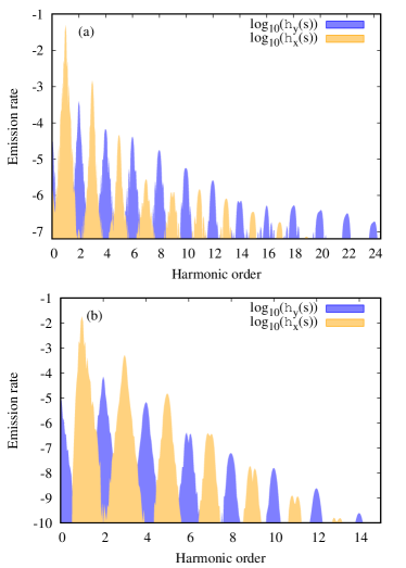
Figure 1: Polarization resolved radiation spectrum via the logarithm of the normalized field strengths $\eta_{x,y}\left(s\right)$ (in arbitrary units): (a) for $\chi=1$, $\Delta=\hbar\omega$, $\varepsilon_{F}=10\Delta$, $\alpha=0.2\mathrm{v}_{x}$; (b) for $F_{0}=1$, $\Delta=10\hbar\omega$, $\varepsilon_{F}=1.2\Delta$ and $\alpha=0.2\mathrm{v}_{x}$.

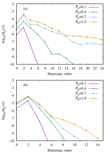
Figure 2: The Fourier content of the topological current. The radiation spectrum induced by Berry curvature for a range of field strengths: (a) for $\Delta=\hbar\omega$, $\varepsilon_{F}=10\Delta$, and $\alpha=0.2\mathrm{v}_{x}$; (b) for $\Delta=10\hbar\omega$, $\varepsilon_{F}=1.2\Delta$, and $\alpha=0.2\mathrm{v}_{x}$.

In Fig. 1 the polarization-resolved radiation spectrum via the logarithm of the normalized field strengths are displayed $\eta_{x,y}\left(s\right)$ at strong pump wave $F_{0}=1$ for semiconductors, and for semimetals. As is seen from this figure, in both cases the higher harmonics due to topological current are dominated over regular ones. This tendency is more strict in the case of semimetals.

The Fourier content of the topological current for a range of field strengths is shown in Fig. 2. We have considered two cases in Fig. 2: $\varepsilon_{F}=10\Delta$ (upper panel) and $\varepsilon_{F}=1.2\Delta$ (lower panel). At low fields, the HHG emission rates decrease rapidly with the order of harmonic. While a much more gradual decrease is observed for semimetals at large $F_{0}$ $\sim 1.0$. This can be explained as follow. It is well known that the Fourier transform is notably sensitive to singularities. The Fourier image of a real analytic function is exponentially decaying at high frequencies.Reed However, if there is a discontinuity, its Fourier image decays according to a power law. The exponent is determined by the type of singularity. As is seen from Eq. (31), for semimetals when $\overline{\Delta}\rightarrow 0$ in the denominator we have singularity which provides plateau for HHG emission rate. For regular current this is well seen for graphene, when $\Delta=0$.Mikhailov To emphasize this finding, in Fig. 3 we plot the Fourier content of radiation induced by the Berry curvature for different Fermi energies at fixed pump wave intensity. As is seen from this figure, with the increasing Fermi energy we have a more gradual decrease in emission rate depending on the harmonic order. In Fig. 3 we have included the case $\varepsilon_{F}=2\Delta$ even though this is clearly outside the intraband regime. However, we want to demonstrate a plateau formation as the gap narrows.

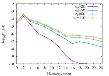
Figure 3: The Fourier content of radiation, induced by the Berry curvature for different Fermi energies at $F_{0}=1$, $\Delta=\hbar\omega$, and $\alpha=0.2\mathrm{v}_{x}$.

The net topological current strongly depends on the tilt parameter $\alpha$. To show this dependence, in Fig. 4 we plot Fourier content of radiation-induced by the Berry curvature at the fixed pump wave intensity $F_{0}=1$ for various values of $\alpha$. For both cases, at moderate harmonics the emission rates $\sim\alpha$ in agreement with Eq. (21). However, at high orders of harmonics this tendency is not preserved. This can be explained from the multipole expansion of the topological current Eq. (25). As is clear from Eq. (25), since $p_{E}\left(t,t^{\prime}\right)\sim\left(\sin\omega t-\sin\omega t^{\prime}\right)$ the current corresponding to ($2s$)-th harmonic besides $D_{x}^{\left(2s-1\right)}$ have contribution from higher moments $D_{x}^{\left(2n-1\right)}$ ($n>s$) of the Berry curvature. The higher moments are more sensitive to Fermi surface deformation which takes place at the change of the tilt parameter $\alpha$. For strong fields, the higher moments of the Berry curvature have sizable contributions that may sum up as constructively as well as destructively. The latter explains the behavior of HHG spectra in Fig. 4 at high orders of harmonics.

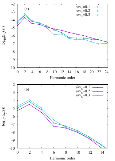
Figure 4: The Fourier content of radiation, induced by the Berry curvature at fixed pump wave normalized field strength $F_{0}=1$ for various values of the tilt parameter $\alpha$: (a) for $\Delta=\hbar\omega$ and $\varepsilon_{F}=10\Delta$; (b) for $\Delta=10\hbar\omega$ and $\varepsilon_{F}=1.2\Delta$.

It is also of interest to more accurately determine the field strength required to achieve a nonperturbative regime of HHG. For this propose in Fig. 5 we display field dependence of scaled nonlinear conductances $\sigma_{y}\left(s\right)=\eta_{y}\left(s\right)/F_{0}^{s-1}$ for the second and fourth harmonics in two cases. In the perturbative limit (27), the $s$th harmonic response via the normalized field strengths $\eta_{y}\left(s\right)$ varies with the field as $\eta_{y}\left(s\right)\propto F_{0}^{s-1}$. Hence, the nonlinear conductances $\sigma_{y}\left(2\right)$ and $\sigma_{y}\left(4\right)$ are field-independent in this limit. The perturbative results are indicated by the solid lines in Fig. 5. As is seen, the full numerical results agree with these predictions in the low field limit. For a semimetal case marked deviations occur at $F_{0}>0.2$ for both second and fourth harmonics. In comparison, for the semiconductor case the transition is at a smaller field of $F_{0}>0.1$. Thus, the threshold field for nonperturbative regime is different for semimetals and for semiconductors, and in addition, the behavior in the nonperturbative regime of HHG is strictly different. For semimetals, the emission rates are increased more rapidly with the increasing pump wave intensity. While for semiconductors the emission rates are increased slowly, thus nonlinear conductances are decreased with the increasing pump wave intensity.

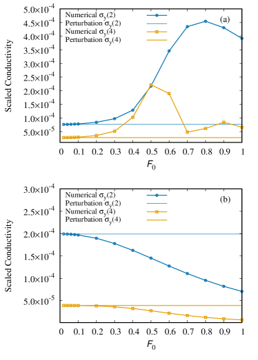
Figure 5: Scaled second and fourth order nonlinear conductances $\sigma_{y}\left(2\right)$ and $\sigma_{y}\left(4\right)$ versus normalized field strength $F_{0}$: (a) for $\Delta=\hbar\omega$, $\varepsilon_{F}=10\Delta$, and $\alpha=0.2\mathrm{v}_{x}$; (b) for $\Delta=10\hbar\omega$, $\varepsilon_{F}=1.2\Delta$, and $\alpha=0.2\mathrm{v}_{x}$.

Let us estimate the pump wave parameters for the considered process of HHG due to topology of bands. The average intensity of the pump wave expressed by $F_{0}$ can be estimated as

$$I=\left(F_{0}\frac{c}{\mathrm{v}_{x}}\frac{\varepsilon_{F}}{\mathrm{eV}}\frac{\hbar\omega}{\mathrm{eV}}\right)^{2}\times 3.\,\allowbreak 4\times 10^{6}\mathrm{\ W\ cm}^{-2},$$

where $c$ is the light speed in vacuum. The typical values of parameters for a semimetal case are: $\mathrm{v}_{x}\approx\mathrm{v}_{y}\approx 4\times 10^{7}\mathrm{cm/s}$, $\Delta\approx 10\mathrm{\ meV}$, $\alpha\approx 0.1\mathrm{v}_{x}$.Sod-Fu Thus, nonperturbative topological HHG will take place at the photon energy $\hbar\omega\approx 10\mathrm{\ meV}$ and intensity $7.\,\allowbreak 6\times 10^{4}\mathrm{\ W\ cm}^{-2}$. The required Fermi energy is $\varepsilon_{F}\approx 0.1\mathrm{eV}$. For the semiconductor case, we assume transition metal dichalcogenides with $\Delta\approx 1\mathrm{\ eV}$ and nonperturbative effects will be essential at $\hbar\omega\approx 0.1\mathrm{eV}$, $\varepsilon_{F}\approx 1.2\mathrm{eV,}$ and the wave intensity $2.\,\allowbreak 7\times 10^{8}\mathrm{\ W\ cm}^{-2}$.

In the end, let us make a remark about the disorder mediated correction to the HHG process. As was shown in Refs.Disorder1 ; Disorder2 ; Disorder3 in addition to the Berry curvature dipole term there exist additional disorder mediated corrections to the second-order nonlinear Hall tensor that have the same scaling in impurity scattering rate. For the nonperturbative regime, this issue demands further consideration. Hence, it is of interest to clear up disorder-induced contributions to the nonperturbative topological HHG. The latter requires extensive numerical analysis and will be the subject of future work.

IV Conclusion

In this paper, the nonlinear optical response of electrons in pseudorelativistic energy bands with nonzero Berry curvature has been investigated. As a model time-reversal invariant system we have considered nanostructures where the Dirac cones are tilted. A semianalytical calculation including all harmonic orders has been presented. We have studied the harmonic content of the induced topological current and have shown that HHG induced solely by the Berry curvature of bands is comparable to regular HHG. At that its polarization is perpendicular to applied pump wave polarization and consequently to regular HHG ones. We have also studied the dependence of the nonlinear response on the driving wave and system parameters for semiconductors and semimetallic cases. It has been shown that in the graphenlike semimetallic cases the topological HHG spectrum has plateau character. The field dependence of the HHG reveals threshold field strengths above which the nonperturbative behavior sets in. Our results apply to a large number of two-dimensional materials where one can achieve the minimum symmetry constraints for a non-vanishing topological current. The corresponding HHG process can thus be used as a way to directly probe and disclose the geometric properties of energy bands in a large number of time-reversal invariant materials. In particular, using multipole expansion of the topological current one can retrieve higher moments of the Berry curvature from the HHG spectrum. This will be more informative beyond the Dirac cone approximation and applicable to the full Brillouin zone.

- (1) E. M. Lifshitz and L. P. Pitaevskii, Statistical Physics: Theory of the Condensed State (Elsevier, Vancouver, 2013), Vol. 9
- (2) R. Karplus and J. M. Luttinger, Phys. Rev. 95, 1154 (1954).
- (3) M. V. Berry, Proc. Roy. Soc. A 392, 45 (1984).
- (4) D. Xiao, M.C. Chang, Q. Niu, Rev. Mod. Phys. 82, 1959 (2010).
- (5) G. Sundaram and Q. Niu, Phys. Rev. B 59, 14915 (1999).
- (6) T. Jungwirth, Q. Niu, and A. H. MacDonald, Phys. Rev. Lett. 88, 207208 (2002).
- (7) F. D. M. Haldane, Phys. Rev. Lett. 93, 206602 (2004).
- (8) N. Nagaosa, J. Sinova, S. Onoda, A. H. MacDonald, and N. P. Ong, Rev. Mod. Phys. 82, 1539 (2010).
- (9) X. Qian, J. Liu, L. Fu, J. Li, Science 346, 1344 (2014).
- (10) M. Z. Hasan and C. L. Kane, Rev. Mod. Phys. 82, 3045 (2010).
- (11) D. Xiao, G.-B. Liu, W. Feng, X. Xu, and W. Yao, Phys. Rev. Lett. 108, 196802 (2012).
- (12) K. F. Mak, K. L. McGill, J. Park, and P. L. McEuen, Science 344, 1489 (2014).
- (13) Y. D. Lensky, J. C. W. Song, P. Samutpraphoot, and L. S. Levitov, Phys. Rev. Lett. 114, 256601 (2015).
- (14) R. V. Gorbachev, J. C. W. Song, G. L. Yu, A. V. Kretinin, F. Withers, Y. Cao, A. Mishchenko, I. V. Grigorieva, K. S. Novoselov, L. S. Levitov, A. K. Geim, Science 346, 448 (2014).
- (15) M. Sui, G. Chen, L. Ma, W.Y. Shan, D. Tian, K. Watanabe, T. Taniguchi, X. Jin, W. Yao, D. Xiao, and Y. Zhang, Nature Phys 11, 1027 (2015).
- (16) L. Li, Y. Yu, G. J. Ye, Q. Ge, X. Ou, H. Wu, D. Feng, X. H. Chen, and Y. Zhang, Nat. Nanotechnol. 9, 372 (2014).
- (17) A. S. Rodin, A. Carvalho, and A. H. Castro Neto, Phys. Rev. Lett. 112, 176801 (2014).
- (18) T. Low, Y. Jiang, and F. Guinea, Phys. Rev. B 92, 235447 (2015).
- (19) E. Witten, Nuovo Cim. Riv. Ser. 39, 313 (2016).
- (20) N. W. Ashcroft and N. D. Mermin, Solid State Physics (Holt, Rinehart and Winston, NY, 1976).
- (21) I. Sodemann and L. Fu, Phys. Rev. Lett. 115, 216806 (2015).
- (22) Q. Ma et al, Nature 565, 337 (2019).
- (23) K. Kang, T. Li, E. Sohn, J. Shan, K. F. Mak, Nat. Mater. 18, 324 (2019).
- (24) D. Dimitrovski, L. B. Madsen, and T. G. Pedersen, Phys. Rev. B 95, 035405 (2017).
- (25) H. K. Avetissian, A. K. Avetissian, A. G. Ghazaryan, G. F. Mkrtchian, and K. V. Sedrakian, J. of Nanophotonics 14, 026004 (2020).
- (26) T. N. Ikeda, Phys. Rev. Research 2, 032015(R) (2020).
- (27) T. G. Pedersen, Phys. Rev. B 95, 235419 (2017).
- (28) H. Liu, Y. Li, Y.S. You, S. Ghimire, T. F. Heinz, and D. A. Reis, Nature Phys. 13, 262 (2017).
- (29) N. Yoshikawa, K. Nagai, K. Uchida, Y. Takaguchi, S. Sasaki, Y. Miyata, K. Tanaka, Nature Commun. 10, 3709 (2019).
- (30) H. K. Avetissian, G. F. Mkrtchian, K. Z. Hatsagortsyan, Phys. Rev. Research 2, 023072 (2020).
- (31) G. Le Breton, A. Rubio, and N. Tancogne-Dejean, Phys. Rev. B 98, 165308 (2018).
- (32) H. K. Avetissian, G. F. Mkrtchian, Phys. Rev. B 99, 085432 (2019).
- (33) H. K. Avetissian, A. K. Avetissian, B. R. Avchyan, G. F. Mkrtchian, Phys. Rev. B 100, 035434 (2019).
- (34) S. Y. Kruchinin, F. Krausz, and V. S. Yakovlev, Rev. Mod. Phys. 90, 021002 (2018).
- (35) J. Schötz, Z. Wang, E. Pisanty, M. Lewenstein, M. F. Kling, and M. F. Ciappina, ACS Photonics 6, 3057 (2019).
- (36) G. F. Mkrtchian, A. Knorr, M. Selig, Phys. Rev. B 100, 125401 (2019).
- (37) R. E. F. Silva, A. Jiménez-Galán, B. Amorim, O. Smirnova, and M. Ivanov, Nat. Photon. 13, 849 (2019).
- (38) D. Bauer and K. K. Hansen, Phys. Rev. Lett. 120, 177401 (2018).
- (39) H. Drüeke and D. Bauer, Phys. Rev. A 99, 053402 (2019).
- (40) T. T. Luu and H. J. Wörner, Nat. Commun. 9, 916 (2018).
- (41) J.-S. You, S. Fang, S.-Y. Xu, E. Kaxiras, and T. Low, Phys. Rev. B 98, 121109(R) (2018).
- (42) Y. Zhang, J. van den Brink, C. Felser, and B. Yan, 2D Materials 5, 044001 (2018).
- (43) B. T. Zhou, C.-P. Zhang, and K. T. Law, Phys. Rev. Applied 13, 024053 (2020).
- (44) J. I. Facio, D. Efremov, K. Koepernik, J.-S. You, I. Sodemann, and J. van den Brink, Phys. Rev. Lett. 121, 246403 (2018).
- (45) R. Battilomo, N. Scopigno, and C. Ortix, Phys. Rev. Lett. 123, 196403 (2019).
- (46) N. M. R. Peres, Yu. V. Bludov, J. E. Santos, A. P. Jauho, and M. I. Vasilevskiy, Phys. Rev. B 90, 125425 (2014).
- (47) L. V. Keldysh, J. Exp. Theor. Phys. 47, 1945 (1964) [Sov. Phys. JETP 20, 1307 (1965)].
- (48) S. A. Mikhailov, Phys. Rev. B 95, 085432 (2017).
- (49) M. Reed and B. Simon, Methods of Modern Mathematical Physics (Academic Press, New York, 1980).
- (50) S. Nandy and I. Sodemann, Phys. Rev. B 100, 195117 (2019).
- (51) Z. Z. Du, C. M. Wang, S. Li, H. Z. Lu, X. C. Xie, Nature Commun. 10, 3047 (2019).
- (52) C. Xiao, Z. Z. Du, and Q. Niu, Phys. Rev. B 100, 165422 (2019).