Pulsar glitch detection with a hidden Markov model

Abstract

Pulsar timing experiments typically generate a phase-connected timing solution from a sequence of times-of-arrival (TOAs) by absolute pulse numbering, i.e. by fitting an integer number of pulses between TOAs in order to minimize the residuals with respect to a parametrized phase model. In this observing mode, rotational glitches are discovered, when the residuals of the no-glitch phase model diverge after some epoch, and glitch parameters are refined by Bayesian follow-up. Here an alternative, complementary approach is presented which tracks the pulse frequency $f$ and its time derivative $\dot{f}$ with a hidden Markov model (HMM), whose dynamics include stochastic spin wandering (timing noise) and impulsive jumps in $f$ and $\dot{f}$ (glitches). The HMM tracks spin wandering explicitly, as a specific realization of a discrete-time Markov chain. It discovers glitches by comparing the Bayes factor for glitch and no-glitch models. It ingests standard TOAs for convenience and, being fully automated, allows performance bounds to be calculated quickly via Monte Carlo simulations. Practical, user-oriented plots are presented of the false alarm probability and detection threshold (e.g. minimum resolvable glitch size) versus observational scheduling parameters (e.g. TOA uncertainty, mean delay between TOAs) and glitch parameters (e.g. transient and permanent jump sizes, exponential recovery time-scale). The HMM is also applied to $\sim 1\,{\rm yr}$ of real data bracketing the 2016 December 12 glitch in PSR J0835$-$4510 as a proof of principle. It detects the known glitch and confirms that no other glitch exists in the same data with size $\gtrsim 10^{-7}f$.

1 Introduction

The exceptional rotational stability of pulsars allows a terrestrial observer armed with an accurate clock to construct a phase-connected timing solution by absolute pulse numbering, even when the observations are irregularly spaced over decades and separated by many pulse periods (Lyne & Graham-Smith, 2012). Traditionally the timing solution is constructed in three stages. (i) The pulse train is folded by cross-correlating against a template profile in the frequency domain to generate a sequence of times-of-arrival (TOAs) (Taylor, 1992). (ii) A phase model is stipulated, which includes frame-of-reference terms (e.g. Solar System barycenter), the pulsar’s intrinsic spin evolution (e.g. spin frequency and its time derivatives, packaged as the coefficients of a Taylor series), astrometric terms (e.g. sky position and proper motion), dispersion in the interstellar plasma, Keplerian orbital elements (if the pulsar is in a binary), and post-Keplerian corrections (Edwards et al., 2006). (iii) The parameters of the phase model are inferred by fitting the TOAs using a weighted least-squares algorithm, such that the residuals are white and minimzed, if the model is perfect. The approach (i)–(iii) has proved highly successful. It forms the backbone of observational studies in pulsar astronomy on a wide range of topics, including tests of general relativity (Taylor, 1992; Stairs, 2003), magnetospheric electrodynamics and coherent emission (Michel, 1991; Melrose, 2017), interstellar scintillation (Rickett, 1990), population synthesis and binary evolution (Faucher-Giguère & Kaspi, 2006), and the search for nanohertz gravitational waves (Lentati et al., 2015; Shannon et al., 2015; Arzoumanian et al., 2016; Hobbs & Dai, 2017).

One intriguing phenomenon revealed by phase-connected timing is rotational glitches: impulsive, erratically occurring, spin-up events which interrupt the secular, electromagnetic spin down of a rotation-powered pulsar. Traditionally a glitch is discovered, when the residuals with respect to a glitchless phase model diverge after a certain epoch, e.g. a jump in spin frequency causes a linear phase ramp. Once the glitch is discovered, two separate, glitchless phase models are fitted to the TOAs before and after the relevant epoch. The differences between the models define the parameters of the glitch, e.g. the jump in spin frequency and its derivatives (Lyne et al., 2000; Espinoza et al., 2011). It is hard to do this uniquely, because the phase evolution includes stochastic spin wandering, known as timing noise (Cordes & Downs, 1985), which is often covariant with glitch-related features like post-glitch recoveries (Lyne et al., 1996). Moreover the gaps between observations can be long and irregular, leading to degeneracies. Work has been undertaken recently to address these issues by applying Bayesian model selection to glitch detection, e.g. using software like temponest (Lentati et al., 2014; Shannon et al., 2016; Yu & Liu, 2017; Lower et al., 2018; Lower et al., 2019). Bayesian methods are promising but relatively expensive; they have not been applied to most pulsars to date.

The physical mechanism that triggers glitch activity remains a mystery; see Haskell & Melatos (2015) for a recent review. Broadly speaking, however, it is thought to involve the sudden relaxation of spin-down-driven elastic stress and differential rotation by local, stick-slip processes such as starquakes (Middleditch et al., 2006; Chugunov & Horowitz, 2010) and superfluid vortex avalanches (Warszawski & Melatos, 2011). In this picture, glitches and their recoveries probe the material properties of bulk matter at nuclear densities, e.g. the shear modulus and superfluid energy gap, under physical conditions which cannot be replicated on Earth (Yakovlev et al., 1999; Lattimer & Prakash, 2007; van Eysden & Melatos, 2010; Watts et al., 2015). In particular, the statistics of glitch sizes and waiting times carry important information (Melatos et al., 2008; Fulgenzi et al., 2017; Ashton et al., 2017; Melatos et al., 2018; Fuentes et al., 2019; Carlin & Melatos, 2019). Expanding the glitch database is essential for achieving a better understanding of the nuclear physics involved.

In this paper, we develop a fast approach to glitch detection and estimation, which complements the existing approach and contributes new insights into performance bounds and spin wandering, as explained in detail in §2. Standard TOAs, generated by cross-correlating the pulse train against a template profile, are still the starting point. Existing software like tempo2 and psrchive can be used unaltered. The TOAs are analysed with a hidden Markov model (HMM), which tracks the underlying evolution of the pulsar’s rotation, including the secular and stochastic components associated with electromagnetic spin down and spin wandering respectively. Glitches are detected by Bayesian model selection, by comparing the evidence for HMMs with and without glitches (cf. temponest). The paper is structured as follows. In §2 we motivate the algorithm by explaining clearly how it fits with existing approaches and what open issues it addresses. In §3 we define the logical components of the HMM-based phase tracker and map each component to its corresponding measurement or model variable in a pulsar timing experiment. In §4 we present and justify an algorithm for converting the HMM output into Bayesian evidence in order to select rigorously between phase models with and without glitches. The performance of the glitch-finding algorithm is then tested. Synthetic data are generated according to the procedure discussed in §5. An introductory worked example is presented in an appendix. Performance metrics such as receiver operating characteristic (ROC) curves are evaluated systematically as functions of the astrophysical and measurement noises, secular spin-down parameters, and glitch parameters in §6. The figures in §6 are designed to be practical. Together they can be used to plan a glitch discovery campaign as a function of experimental variables such as TOA uncertainties and the desired measurement resolution, e.g. of glitch sizes and recovery time-scales.

The paper is framed as a method paper. Most of the tests are done on synthetic data deliberately, to study the behavior of the algorithm under controlled conditions. The next step is to apply the HMM to real data, a larger project which is under way. A quick foretaste of what is possible in presented in §7 using public data from PSR J0835$-$4510 as a worked example. Theoretical aspects of the algorithm are explored further by Suvorova et al. (2018) in a general signal processing context.

2 Motivation

Before introducing the HMM in §3 we explain firstly what issues in glitch detection the new algorithm seeks to address, under what circumstances it proves useful (and when it does not), and how it complements traditional glitch detection methods. Existing approaches enjoy a long record of success, so it is important to articulate what specific contributions the new algorithm makes. The main contributions are (i) a fast recipe for generating systematic performance bounds, and (ii) a sophisticated way to distinguish spin wandering and glitches.

Some interesting questions remain unanswered about the performance bounds of traditional glitch searches based on software packages such as tempo2 (Hobbs et al., 2006; Edwards et al., 2006), psrchive (van Straten et al., 2012), temponest (Lentati et al., 2014), and their relatives. Given the spin wandering amplitude and TOA measurement uncertainty in a particular pulsar, as well as a glitch size detection threshold, what is the false alarm probability, when a traditional glitch search is performed? Are all catalogued glitches real (see footnote 1), or are some of the smaller events actually spin wandering (Jones, 1990; D’Alessandro et al., 1995; Janssen & Stappers, 2006; Yu & Liu, 2017)? What is the smallest event that a traditional glitch search can detect, as a function of the false alarm and false dismissal probabilities? How does the detection limit vary between objects with different spin wandering amplitudes? Some work has been done to develop quantitative answers to these questions. Janssen & Stappers (2006) conducted Monte Carlo simulations to estimate the minimum glitch size resolvable in PSR J1740$-$3015; see also Watts et al. (2015) with reference to the Square Kilometer Array. Shannon et al. (2016) and Lower et al. (2018) reanalysed TOAs from PSR J0835$-$4510 and PSR J1709$-$4429 respectively within a Bayesian framework to look for false alarms and false dismissals, and a similar, multi-object project is under way using data collected by the Molonglo Observatory Synthesis Telescope (Jankowski et al., 2019; Lower et al., 2019). Yu & Liu (2017) performed the largest study of glitch detection probabilities so far, again within a Bayesian framework, involving 165 pulsars timed by the Parkes Observatory between 1990 and 2011 (Yu et al., 2013; Yu & Liu, 2017). The latter authors argued persuasively, that the study should be extended to more pulsars. However, the task is not easy. One rigorous approach in signal processing is to construct a ROC curve for the search algorithm in question, by plotting the detection probability against the false alarm probability. This entails many Monte Carlo simulations, which are prohibitive to analyse, when traditional algorithms still rely on human supervision (e.g. by-eye inspection of post-fit residuals) even when aided by software like temponest. Crowdsourcing offers one possible solution, perhaps by leveraging the infrastructure of the PULSE@Parkes project (Hobbs et al., 2009), but it brings its own logistical challenges. Consequently few if any ROC curves have been published for traditional glitch finding schemes.

How does the new algorithm relate to traditional methods of glitch detecton? The HMM formulation shares some common features with recent work developing a new, Bayesian, pulsar timing infrastructure based on pulse domain analysis and/or model selection (Lentati et al., 2014; Lentati et al., 2015; Lentati & Shannon, 2015; Lentati & et al., 2017; Lentati et al., 2017, 2018; Ashton et al., 2019). The main similarity is that a glitch is discovered, when the Bayes factor comparing glitch and no-glitch phase models surmounts a user-selected threshold, as with temponest. However there are differences. (i) The HMM plugs into the traditional infrastructure for generating TOAs. It does not operate in the pulse domain, in order to maximize the use of existing software. It can be extended to the pulse domain in the future, if there is enough demand. (ii) The HMM does not treat spin wandering as “noise”; it tracks it explicitly. In other words, it evaluates the likelihood of the specific spin wandering pattern observed (i.e. a specific realization of a discrete-time Markov chain, in the language of stochastic processes), whereas temponest and related algorithms analyse the ensemble statistics of the spin wandering [e.g. the timing noise power spectral density (Coles et al., 2011)]. (iii) The HMM is fast. It requires $\sim 10^{12}$ floating point operations [$\sim 0.1$ central processing unit (CPU) hours] per target per year of observations, starting from an approximate, glitchless timing solution generated by traditional methods.

We emphasize that the approach developed here does not supplant traditional timing methods nor the newer pulse domain approach. All three approaches complement each other and are more powerful when deployed in tandem. For example, when the goal is to measure a slow, secular phase evolution described faithfully by a Taylor expansion (e.g. in binary pulsar tests of general relativity), the HMM formulation is unnecessary, because there is no covariance between stochastic spin wandering and the secular dynamics (e.g. binary orbital decay). On the other hand, when spin wandering is covariant with other short-time-scale phenomena like glitches and their recoveries, the HMM offers an alternative perspective on whether a glitch occurs, by tracking the spin wandering directly within systematic performance bounds, while ingesting standard TOAs for the sake of convenience.

3 Phase tracking

A HMM is a scheme for inferring the trajectory of a system through a sequence of unobservable (hidden) states by measuring observables related probabilistically to the hidden states. In the pulsar context, the observables are the TOAs, and the hidden state is the underlying rotational state of the pulsar (e.g. its spin frequency and instantaneous derivatives with respect to time), which cannot be measured uniquely from a single TOA or the interval between a TOA pair. In §3.1, we describe how to formulate the pulsar timing problem in terms of a HMM, which converts TOAs into a phase-connected timing solution. The state structure of the HMM is defined precisely in §3.2. We then relate the TOAs probabilistically to the pulsar’s rotational state in §3.3 and describe how the rotational state evolves stochastically under the action of electromagnetic spin down, timing noise, and glitches in §3.4. Resolution and gridding issues are discussed in 3.5. An efficient algorithm for solving the HMM numerically is set out in Appendix A. The presentation follows closely the formal derivation by Suvorova et al. (2018).

3.1 HMM formulation

A HMM is a probabilistic finite-state automaton specified by a hidden state variable $q(t)$, which can take on $N_{Q}$ discrete values; an observation variable $o(t)$, which is not necessarily discrete; and a sequence of times $t_{1}\leq\dots\leq t_{N_{T}}$ when snapshots of the system are taken. In general, $q(t_{n})$ and $o(t_{n})$ are multi-dimensional vectors, and the times $t_{n}$ are unequally spaced.

The probability for the system to jump from hidden state $q_{i}$ at time $t_{n}$ to hidden state $q_{j}$ at time $t_{n+1}$ is called the transition probability. It is given by

$$A_{q_{j}q_{i}}={\rm Pr}[q(t_{n+1})=q_{j}|q(t_{n})=q_{i}]~{}.$$ (1)

The probability of measuring the datum $o(t_{n})$ at time $t_{n}$, if the system is in state $q(t_{n})=q_{i}$, is called the emission probability. It is given by

$$L_{o(t_{n})q_{i}}={\rm Pr}[o(t_{n})|q(t_{n})=q_{i}]~{}.$$ (2)

Writing $Q_{1:N_{T}}=\{q(t_{1}),\dots,q(t_{N_{T}})\}$ and $O_{1:N_{T}}=\{o(t_{1}),\dots,o(t_{N_{T}})\}$, we can express the total probability that the observed sequence $O_{1:N_{T}}$ arises from the hidden sequence $Q_{1:N_{T}}$ as

$$\Pr(Q_{1:N_{T}}|O_{1:N_{T}})=\Pi_{q(t_{1})}L_{o(t_{1})q(t_{1})}\prod_{n=2}^{N_{T}}A_{q(t_{n})q(t_{n-1})}L_{o(t_{n})q(t_{n})}~{},$$ (3)

where

$$\Pi_{q_{i}}={\rm Pr}[q(t_{1})=q_{i}]$$ (4)

denotes the prior probability.

Three essential questions of practical value can be asked about a HMM of the above form (Rabiner, 1989; Quinn & Hannan, 2001). First, given the observed sequence $O_{1:N_{T}}$ and a model $M=\{A_{q_{j}q_{i}},L_{o(t_{n})q_{i}},\Pi_{q_{i}}\}$, what is $\Pr(O_{1:N_{T}}|M)$, i.e. what is the Bayesian evidence for $M$? Knowing $\Pr(O_{1:N_{T}}|M)$, one can select between different models. Second, given $O_{1:N_{T}}$ and $M$, what is the optimal hidden sequence $Q_{1:N_{T}}$ which best explains the data according to some meaningful metric? Third, given $O_{1:N_{T}}$, what model $M$ maximizes $\Pr(O_{1:N_{T}}|M)$?

The first and second questions in the previous paragraph are fundamental to the glitch-finding problem studied in this paper. Efficient algorithms to solve them are presented in Appendix A and assembled into a systematic glitch-finding scheme in §4. There is no unique answer to the second question. One possible solution is $Q_{1:N_{T}}^{\ast}={\rm arg\,max\,}\Pr(Q_{1:N_{T}}|O_{1:N_{T}},M)$, which maximizes $\Pr(Q_{1:N_{T}}|O_{1:N_{T}},M)$ sequence-wise (Quinn & Hannan, 2001). Another possible solution is $\hat{q}(t_{n})={\rm arg\,max\,}\Pr[q(t_{n})|O_{1:N_{T}},M]$ for $1\leq n\leq N_{T}$, which maximizes $\Pr[q(t_{n})|O_{1:N_{T}},M]$ point-wise (Rabiner, 1989). The third question, which corresponds here to learning a dynamical model of glitches statistically from the data, can be solved by iterative methods like the Baum-Welch algorithm (Rabiner, 1989) but lies outside the scope of this work.

3.2 Summary of HMM components

In the pulsar timing context, the components of the HMM are the following.

1. Hidden state. In this paper, we track the instantaneous frequency $f(t)$ and its first time derivative $\dot{f}(t)$. Future work can easily include higher-order derivatives, e.g. the secular component of the second derivative $\langle\ddot{f}\rangle=n\dot{f}^{2}/f$ describing electromagnetic braking, where $1\lesssim n\leq 3$ is the electromagnetic braking index (Melatos, 1997; Archibald et al., 2016). The stochastic component of $\ddot{f}$, whose magnitude usually exceeds $n\dot{f}^{2}/f$ (Arzoumanian et al., 1994; Johnston & Galloway, 1999), is absorbed in the wandering of $f$. We also define (but do not track; see §3.4 and §4) a Boolean variable, $g(t)$, which equals unity if a glitch occurs at time $t$ and zero otherwise. In summary, therefore, the hidden state is $q(t)=[f(t),\dot{f}(t),g(t)]$.

2. Observable. In this paper, the HMM time sequence $\{t_{1},\dots,t_{N_{T}}\}$ is defined to map one-to-one onto the measured, unequally spaced TOAs, starting from the second TOA. The measurement variable at time $t_{n}$ is defined to equal the displacement between consecutive TOAs, viz. $o(t_{n})=t_{n}-t_{n-1}$, where $t_{0}$ corresponds to the first TOA; henceforth we write $x_{n}=t_{n}-t_{n-1}$ for brevity. Future refinements include augmenting $o(t_{n})$ with auxiliary information, e.g. tagging it with the pulse period measured locally at each TOA.

3. Emission probability. Given $x_{n}$ and an associated measurement error, whose variance equals $2\sigma_{\rm TOA}^{2}$, there exists a limited but degenerate set of $(f,\dot{f})$ pairs, which produce an integer number of pulses in the interval $x_{n}$. An explicit formula for the emission probability for arbitrary $f$ and $\dot{f}$ and Gaussian measurement errors is given in §3.3 in terms of the von Mises distribution. By way of illustration, in the artificial special case with $\dot{f}=0$ and $\sigma_{\rm TOA}=0$, the emission probability is proportional to a sum of delta functions, $\delta(f-1/x_{n})+\delta(f-2/x_{n})+\dots$.

4. Transition probability. In this paper, we track the rotational phase on three time-scales: (i) secular, electromagnetic braking on the longest time-scale, $f/\dot{f}\gtrsim 10^{3}\,{\rm yr}$, which greatly exceeds the total observation span, $T_{\rm obs}\lesssim 10^{2}\,{\rm yr}$; (ii) spin wandering (timing noise) on an intermediate time-scale, stretching from days to years (Cordes & Downs, 1985; Price et al., 2012; Namkham et al., 2019; Parthasarathy et al., 2019; Goncharov et al., 2019; Lower et al., 2020); and (iii) glitches, i.e. unresolved jumps in $f$ and $\dot{f}$, whose rise times are much shorter than $\min_{n}x_{n}$. The stochastic dynamics of $q(t)=[f(t),\dot{f}(t),g(t)]$, which determine $A_{q_{j}q_{i}}$, are modeled as biased Brownian motion with process variance per unit time $\sigma^{2}$ via a Langevin equation in §3.4 and Appendix B. Note that glitches are often followed by quasiexponential recoveries, which last days to years (van Eysden & Melatos, 2010). The recoveries can be incorporated into the phase model in future work. Here we absorb them into the timing noise, which occurs on a similar time-scale, and show a posteriori that this is an effective approach in practice, with the algorithm successfully detecting glitches in synthetic data containing recoveries (see §5).

5. Prior. A uniform prior is adopted on $f$ and $\dot{f}$ within a restricted domain, known as the domain of interest (DOI; see §3.5). Practically the DOI for any pulsar is defined by traditional phase-connected timing methods, e.g. a standard tempo2 fit, as well as prior astrophysical knowledge, e.g. population-based constraints on glitch sizes (Melatos et al., 2008; Espinoza et al., 2011; Howitt et al., 2018). In general $\Pr(Q_{1:N_{T}}|O_{1:N_{T}})$ is insensitive to the choice of a uniform prior, because $\Pi_{q_{i}}$ is just one factor out of $2N_{T}\gg 1$ in what is usually a large product in (3) (Suvorova et al., 2016, 2017; Abbott et al., 2017).

3.3 Emission probability

Given a displacement $x_{n}$, what can we say probabilistically about the rotational state of the pulsar at $t_{n}$? For $\dot{f}(t_{n})=0$, without measurement noise, we can infer the instantaneous frequency, $f(t_{n})$, to be an integer multiple of $x_{n}^{-1}$. For $\dot{f}(t_{n})\neq 0$, a particular combination of $x_{n}$, $f(t_{n})$, and $\dot{f}(t_{n})$ is inferred to be an integer. The combination is unique, as long as $x_{n}$ is short enough (see below). When measurement noise is switched on, these statements continue to hold true, but the estimates are “fuzzy”.

In the absence of measurement noise and discontinuous glitches, and with $\ddot{f}=0$ over a short enough time-scale, we can approximate the frequency evolution in the interval $t_{n-1}\leq t\leq t_{n}$ as a backward Taylor series, $f(t)=f(t_{n})+(t-t_{n})\dot{f}(t_{n})$, and then integrate $d\phi/dt=2\pi f(t)$ to get the phase,

$$\phi(t_{n})=\phi(t_{n-1})+2\pi x_{n}f(t_{n})-\pi x_{n}^{2}\dot{f}(t_{n})~{}.$$ (5)

The minus sign in the last term arises, because we use a backward difference scheme. Let $N_{n}$ be the number of pulses between $t_{n-1}$ and $t_{n}$. By the definition of the TOAs, $N_{n}$ is an integer, and we have $N_{n}=\Phi(x_{n})$ with $\Phi(x_{n})=x_{n}f(t_{n})-x_{n}^{2}\dot{f}(t_{n})/2$. This equation corresponds to a line in the $f(t_{n})$-$\dot{f}(t_{n})$ plane given $x_{n}$ and $N_{n}$.

If each TOA has a Gaussian measurement error with zero mean and variance $\sigma_{\rm TOA}^{2}$, then $x_{n}$ also has a Gaussian measurement error, denoted by $w_{n}$, with twice the variance. We write the measurement equation as

$$x_{n}=\Phi^{-1}(N_{n})+w_{n}~{},$$ (6)

where $\Phi^{-1}$ is the inverse function of $\Phi$, not its reciprocal. In practice, $x_{n}$ is always short enough, i.e. $x_{n}\ll 2f(t_{n})/|\dot{f}(t_{n})|$, so that $\Phi$ is uniquely invertible up to an integer multiple. The inversion is unique, even when the timing noise is strong ($|\ddot{f}|\gg n\dot{f}^{2}/f$), unlike higher-order Taylor expansions, where the inversion is multi-valued (modulo the integer multiples) for $x_{n}^{2}\gtrsim 6f(t_{n})/|\ddot{f}(t_{n})|$. In this paper, timing noise is tracked explicitly via the HMM transition probability, as described in §3.4.

The emission probability is proportional to the probability density function (PDF) of the observed variable $x_{n}$. Suvorova et al. (2018) showed that the PDF of $\Phi(x_{n})$ is approximately a wrapped Gaussian, because the phase is $2\pi$-periodic; see Appendix A of the latter reference. Suvorova et al. (2018) also showed that the wrapped Gaussian can be approximated accurately by a von Mises distribution (Mardia & Jupp, 2009), which is more convenient to evaluate numerically. Hence one can write

$$L_{x_{n}q(t_{n})}=[2\pi I_{0}(\kappa)]^{-1}\exp\{\kappa\cos[2\pi\Phi(x_{n})]\}$$ (7)

with

$$\kappa=[2\sigma_{\rm TOA}^{2}f(t_{n})^{2}]^{-1}~{}.$$ (8)

In (7), $I_{0}(\kappa)$ symbolizes a modified Bessel function of the first kind. It is approximated by $I_{0}(\kappa)\approx(2\pi\kappa)^{-1/2}\exp(\kappa)$ in the regime $\kappa\gg 1$ to avoid underflow errors in the computation. Intuitively $\kappa^{-1/2}$ is the number of pulses squeezed into a time interval lasting as long as the uncertainty in $x_{n}$. Note that the hidden state $q(t_{n})$ enters (7) through $\Phi(x_{n})$, which depends on $f(t_{n})$ and $\dot{f}(t_{n})$. By contrast, $N_{n}$ does not enter (7) explicitly; the HMM does not count the number of pulses in the interval $t_{n-1}\leq t\leq t_{n}$ explicitly, although this information can always be extracted post factum using (6), once the HMM is solved to obtain $Q_{1:N_{T}}$.

Figure 1 displays a sample of $L_{x_{n}q(t_{n})}$ contours in the $f(t_{n})$-$\dot{f}(t_{n})$ plane for two $x_{n}$ values. Each stripe corresponds to a peak of $L_{x_{n}q(t_{n})}$ along the line $N_{n}=\Phi(x_{n})=(2\pi)^{-1}[x_{n}f(t_{n})-x_{n}^{2}\dot{f}(t_{n})/2]$. Its slope, $2/x_{n}$, decreases as $x_{n}$ increases. Formally speaking, equation (7) has an infinite number of equal-height peaks, each corresponding to an integer value of $N_{n}$. In practice, the number of peaks within the DOI (drawn arbitrarily here as the figure frame) is finite. Without extra information, e.g. a phase-connected solution constructed by traditional means, all the peaks are equally likely. As $x_{n}$ increases three-fold from the left panel to the right panel, two things happen: the minimum $f(t_{n})$ (corresponding to $N_{n}=1$) decreases, and the separation of the peaks decreases. On the one hand, therefore, there is greater ambiguity, because there are more peaks to interrogate in the DOI. On the other hand, the estimate of $q(t_{n})$ is more accurate, once the HMM finds the optimal peak, because the peaks are narrower. In Figure 1, the number of yellow stripes in the frame increases from two to 18, as $x_{n}$ increases from $1\times 10^{5}\,{\rm s}$ in the left panel to $3\times 10^{5}\,{\rm s}$ in the right panel. The full-width half-maximum (FWHM) per stripe projected on the $\dot{f}(t_{n})$ axis decreases from $7.2\times 10^{-11}\,{\rm Hz\,s^{-1}}$ in the left panel to $7.9\times 10^{-12}\,{\rm Hz\,s^{-1}}$ in the right panel.

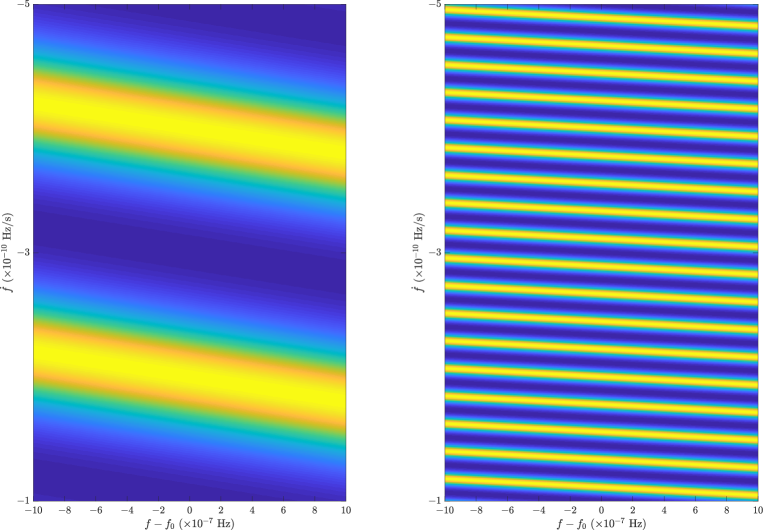
Figure 1: Contour map of the emission probability $L_{x_{n}q(t_{n})}$ [equation (7)] (arbitrary color scale; yellow high, blue low) as a function of the hidden state components $f(t_{n})$ (units: Hz) and $\dot{f}(t_{n})$ (units: ${\rm Hz\,s^{-1}}$) for measurements $x_{n}=1\times 10^{5}\,{\rm s}$ (left panel) and $x_{n}=3\times 10^{5}\,{\rm s}$ (right panel). Both panels are centered on $(f_{0},\dot{f}_{0})=(5\,{\rm Hz},-3\times 10^{-10}\,{\rm Hz\,s^{-1}})$. Measurement uncertainty: $\sigma_{\rm TOA}^{2}=2\times 10^{-2}\,{\rm s^{2}}$, i.e. $\kappa=1$.

Equations (7) and (8) assume that the state space is continuous. In practice, the $f(t_{n})$-$\dot{f}(t_{n})$ plane is divided into a grid. A generalized version of (8) that accounts for gridding and lets $\sigma_{\rm TOA}$ vary with $t_{n}$ is discussed in §3.5.

3.4 Transition probability

The equation of motion obeyed by $q(t)=[f(t),\dot{f}(t),g(t)]$ in a real pulsar is unknown. Instead we construct an idealized model for how $q(t)$ evolves during the HMM step $t_{n-1}\leq t\leq t_{n}$. Away from a glitch, we assume that the system obeys a continuous Wiener process described by the Langevin equation

$$\frac{d^{2}f}{dt^{2}}=\xi(t)~{},$$ (9)

where $\xi(t)$ is a fluctuating torque derivative with white noise statistics satisfying $\langle\xi(t)\rangle=0$ and $\langle\xi(t)\xi(t^{\prime})\rangle=\sigma^{2}\delta(t-t^{\prime})$, and $\sigma$ is a tunable parameter (units: ${\rm Hz\,s^{-3/2}}$). At the instant when a glitch occurs, the continuous evolution is interrupted, and $f(t)$ and $\dot{f}(t)$ undergo impulsive permanent changes $\Delta f_{\rm p}$ and $\Delta\dot{f}_{\rm p}$ respectively.

We emphasize that (9) is designed mainly with the practical needs of the HMM in mind; it should not be viewed as a physical model of a pulsar. Nevertheless it does embody the three physical time-scales discussed in point 4 in §3.3: long (electromagnetic braking), intermediate (timing noise), and short (glitches). Electromagnetic braking enters through the initial conditions; the secular spin-down torque sets $\dot{f}(t_{n-1})$. We neglect $\langle\ddot{f}\rangle=n\dot{f}^{2}/f$ in (9) as discussed in §3.2. Timing noise enters through the right-hand side of (9). Its amplitude is set by $\sigma$, which satisfies $\langle[\dot{f}(t_{n})-\dot{f}(t_{n-1})]^{2}\rangle=\sigma^{2}x_{n}$ as for any Wiener process. Glitch-driven jumps in the frequency and frequency derivative enter through the initial conditions $f(t_{n-1})$ and $\dot{f}(t_{n-1})$ respectively. Glitches can occur anywhere within a TOA gap, because a discrete-time HMM only registers state changes at $t_{1},\dots,t_{N_{T}}$ by definition. The TOA gap defines the uncertainty on the estimated glitch epoch, once the HMM detects a glitch. Note that $\xi(t)$ corresponds to a fluctuating torque derivative, whereas theories of timing noise often invoke a fluctuating torque (Cordes, 1980; Cordes & Downs, 1985; Melatos & Peralta, 2010; Melatos & Link, 2014) as well as frequency and phase fluctuations (Cordes, 1980). The distinction is unimportant in many HMM tracking problems. The degree to which it matters when doing model selection, as in this paper, is tested empirically in §6.

The forward Fokker-Planck equation corresponding to (9) can be solved to find the PDF of $q(t_{n})$ given $q(t_{n-1})$ (Gardiner, 1994), as required by (3). The result, derived in Appendix B, is

$$A_{q(t_{n})q(t_{n-1})}=(2\pi)^{-1/2}|{\rm det}\Sigma|^{-1/2}N_{G}^{-1}\sum_{(\Delta f_{\rm p},\Delta\dot{f}_{\rm p})\in G}\exp\{-[q(t_{n})-\mu]^{\rm T}\Sigma^{-1}[q(t_{n})-\mu]\}~{},$$ (10)

where the superscript T denotes the matrix transpose, the secular evolution is described by the mean vector $\mu=(\mu_{f},\mu_{\dot{f}})$, with

$$\mu_{f} = f(t_{n-1})+x_{n}\dot{f}(t_{n-1})+g(t_{n-1})(\Delta f_{\rm p}+x_{n}\Delta\dot{f}_{\rm p})~{},$$ (11)

$$\mu_{\dot{f}} = \dot{f}(t_{n-1})+g(t_{n-1})\Delta\dot{f}_{\rm p}~{},$$ (12)

the dispersion is described by the covariance matrix,

$$\Sigma=\sigma^{2}\left(\begin{tabular}[]{cc}$x_{n}^{3}/3$&$x_{n}^{2}/2$\\ $x_{n}^{2}/2$&$x_{n}$\end{tabular}\right)~{},$$ (13)

and $\Sigma^{-1}$ is the matrix inverse of $\Sigma$. In (10), $G=G[g(t_{n-1})]$ denotes the set of jump pairs $(\Delta f_{\rm p},\Delta\dot{f}_{\rm p})$ searched by the HMM at step $t_{n-1}$, and $N_{G}$ is the cardinality of $G$. If a glitch does not occur, we have $g(t_{n-1})=0$, $\Delta f_{\rm p}=0$, $\Delta\dot{f}_{\rm p}=0$, and $N_{G}=1$. If a glitch does occur, $\Delta f_{\rm p}$ and $\Delta\dot{f}_{\rm p}$ are constrained to lie within the DOI defined by astrophysical priors, e.g. historical glitch observations, and $N_{G}$ is determined by the grid resolution within the DOI (see §3.5).

Figure 2 displays a sample of $A_{q(t_{n})q(t_{n-1})}$ contours in the $f(t_{n})$-$\dot{f}(t_{n})$ plane for a representative choice of $q(t_{n-1})$ (centered on the red dot in each panel) and two values each of $x_{n}$ and $\sigma$. Every cross-centered ellipse in the figure corresponds to one term in (10), i.e. one choice of $\Delta f_{\rm p}$ and $\Delta\dot{f}_{\rm p}$ in $G$ and the DOI. The principal axes of the ellipses are determined by $x_{n}$ through the covariance matrix $\Sigma$, as can be seen by comparing the left ($x_{n}=1\times 10^{5}\,{\rm s}$) and right top ($x_{n}=2\times 10^{5}\,{\rm s}$) panels. The ellipse marked with a red diamond corresponds to no glitch, i.e. $g(t_{n-1})=0$; the other ellipses have $g(t_{n-1})=1$. The DOI is drawn artificially small, so that the reader can see its boundaries within the figure while still making out the ellipses individually; in practice one would expect typically $\gtrsim 10^{3}$ ellipses within the frame of Figure 2. For $\sigma$ relatively low, as in the left panel, the ellipses are narrow and nearly disjoint. For $\sigma$ relatively high, as in the right bottom panel, the ellipses broaden and overlap; $\sigma$ increases five-fold in passing from the left to the right bottom panel. In the high-$\sigma$ regime, $A_{q(t_{n})q(t_{n-1})}$ can be approximated as uniform across the DOI for $g(t_{n-1})=1$, with all glitch terms contributing equally to the sum in (10), while the $g(t_{n-1})=0$ term stands apart.

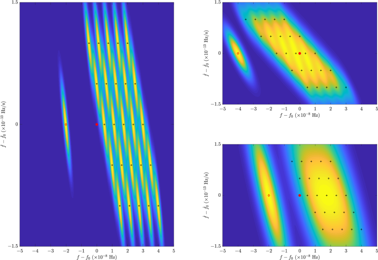
Figure 2: Contours of the transition probability $A_{q(t_{n})q(t_{n-1})}$ (arbitrary color scale; yellow high, blue low) plotted versus the endpoint $f(t_{n})$ and $\dot{f}(t_{n})$ of a HMM step. The axes are centered on the red dot at $q(t_{n-1})=(f_{0},\dot{f}_{0})=(5\,{\rm Hz},-2\times 10^{-13}\,{\rm Hz\,s^{-1}})$. Every cross-centered ellipse corresponds to one term in (10), i.e. one combination of $\Delta f_{\rm p}$ and $\Delta\dot{f}_{\rm p}$ if a glitch occurs at $t_{n-1}$. The allowed jumps in the set $G$ are restricted to the ranges $2.5\leq\Delta f_{\rm p}/(10^{-8}\,{\rm Hz})\leq 5.0$ and $-1.0\leq\Delta\dot{f}_{\rm p}/(10^{-13}\,{\rm Hz\,s^{-1}})\leq 1.0$ for the sake of readability. The red diamond indicates the probability peak, when no glitch occurs at $t_{n-1}$. (Left panel.) $x_{n}=1\times 10^{5}\,{\rm s}$, $\sigma=1\times 10^{-16}\,{\rm Hz\,s^{-3/2}}$. (Right top panel.) $x_{n}=2\times 10^{5}\,{\rm s}$, $\sigma=1\times 10^{-16}\,{\rm Hz\,s^{-3/2}}$. (Right bottom panel.) $x_{n}=1\times 10^{5}\,{\rm s}$, $\sigma=5\times 10^{-16}\,{\rm Hz\,s^{-3/2}}$.

The Boolean component $g(t)$ of $q(t)$ does not appear explicitly in (9); in other words, we do not track it. Partly this is because its true evolution is unknown. Are glitches a Poisson process, for instance, and what is the rate? Empirically some pulsars show Poisson-like glitch activity, but others do not (Melatos et al., 2008; Espinoza et al., 2011; Howitt et al., 2018; Fuentes et al., 2019). Moreover, it is inefficient computationally to track $g(t)$. Historical glitch data imply $g(t)=0$ most of the time, with one glitch being discovered among every $\gtrsim 10^{3}$ TOAs, at least for glitches of a size that traditional timing methods can resolve (Janssen & Stappers, 2006). In this paper, therefore, we do not assume anything about the distribution of glitch waiting times. Instead we incorporate $g(t)$ into the Bayesian model selection procedure described in §4. We run the HMM for a glitchless model with $g(t_{n})=0$ and a single-glitch model with $g(t_{n})=\delta_{nk}$ for fixed $k$ ($1\leq n\leq N_{T}$) and compute the odds ratio to test for the existence of a glitch at $t_{k}$. We then repeat the exercise $N_{T}$ times for $1\leq k\leq N_{T}$. A full discussion of the procedure is given in §4 and Appendix A.

Quasiexponential post-glitch recoveries do not feature in the hidden state evolution described by (9)–(13), even though they are observed in reality. In this paper, we include post-glitch recoveries in the synthetic data generated according to §5 and show that the HMM performs well at finding synthetic glitches with recoveries, even though the recoveries are not built into $A_{q_{j}q_{i}}$. Of course $A_{q_{j}q_{i}}$ can be extended to include recoveries, at the expense of introducing at least two extra parameters into the HMM model, viz. recovery fraction and recovery time-scale, and weakening the Markov approximation. Neither parameter is known a priori and would need to be searched over, increasing the complexity of the HMM. We postpone developing this capability, until the data sets grow to the point, when it is genuinely needed.

3.5 Grid resolution and DOI

The DOI relevant to a particular pulsar is the region in the $f$-$\dot{f}$ plane that contains all possible hidden state sequences $Q_{1:N_{T}}$ consistent with the observed TOAs. The set of hidden states is constructed by dividing the DOI into a grid, whose spacing is chosen to resolve essential features like electromagnetic spin down, timing noise, and glitches (see §3.2). In Appendix C we offer one practical recipe for gridding the DOI. It is not unique; the reader is encouraged to modify it, as the experiment demands. We distinguish carefully between the DOI and the set $G$ in (10). The DOI encompasses the trajectories of the HMM, starting from the subset of the $f$-$\dot{f}$ plane covered by the uniform prior (see §3.2). It is chosen at the outset so that it does not exclude any admissible HMM trajectory consistent with the observed TOAs and the phase model in §3.4. In contrast, $G$ defines the set of glitch-related jumps in $q(t)$ consistent with §3.4 and the requirement that $q(t)$ stays within the DOI at all times. It is updated at each $t_{n}$ and depends on $q(t_{n-1})$ via (10). Appendix C describes how discretization affects $G$ and modifies the formulas (7) and (8) for the emission probability.

4 Glitch detection by Bayesian model selection

Once the phase tracker in §3 is implemented, the task of discovering a glitch reduces to comparing, given the data, the probability of a phase model with one or more glitches against the probability of a glitchless phase model. From a Bayesian perspective, the comparison reduces to calculating the evidence ratio (or marginal likelihood ratio) of the competing models. In §4.1 and Appendix A, we describe how to calculate the evidence ratio using the HMM forward algorithm. In §4.2 we generalize the evidence ratio calculation to multiple glitches. In §4.3 and Appendix A, we describe how to infer the optimal ephemeris using the HMM forward-backward algorithm, once the preferred model (the one with the highest evidence ratio) is identified. The preferred model may or may not contain a glitch. In §4.4 we present a preliminary survey of the computational cost. Finally, for the sake of completeness, we outline briefly in Appendix D a related approach to discovering glitches, known as a jump Markov model, and explain why it is not used here.

The HMM does not prefer a particular physical model of glitches. Any physical mechanism which conforms to the idealized transition probability (10)–(13) falls within the ambit of the HMM. Equations (10)–(13) take a generic form and are motivated observationally, so they automatically embrace many microphysical mechanisms, which have been developed to explain observed glitch activity, including superfluid vortex avalanches (Anderson & Itoh, 1975; Warszawski & Melatos, 2011), starquakes (Middleditch et al., 2006; Chugunov & Horowitz, 2010), and hydrodynamic instabilities (Glampedakis & Andersson, 2009); see Haskell & Melatos (2015) for a recent review. Equations (10)–(13) also embrace many microphysics-agnostic meta-models, which have been developed to make falsifiable predictions about long-term glitch statistics (Fulgenzi et al., 2017; Melatos et al., 2018; Carlin & Melatos, 2019). In this sense, the HMM is robust towards physical mechanisms in the literature; it accommodates all the main classes. By the same token, it cannot discriminate between the classes; that is not its function; it is a glitch detector, not a sieve for physical mechanisms. In what follows, the term “model” refers to a sequence $g(t_{0}),\dots,g(t_{N_{T}-1})$ admissible by the Markov process (10)–(13), not a codification of a physical mechanism. The sequence preferred by the data is the one with the highest evidence ratio, as noted above and in §4.1. The reader is encouraged to experiment with alternatives to (10)–(13) and explore their effect on glitch detection.

4.1 Model evidence

Let $M_{0}$ denote the model, where no glitch occurs in the interval $t_{0}\leq t\leq t_{N_{T}}$, i.e. we have $g(t_{n-1})=0$ for all $1\leq n\leq N_{T}$. Let $M_{1}(k)$ denote the model, where one glitch occurs in the interval $t_{k-1}\leq t\leq t_{k}$, i.e. we have $g(t_{n-1})=\delta_{nk}$ for all $1\leq n\leq N_{T}$ ($\delta_{nk}$ is the Kronecker delta symbol). Let $M_{2}(k,l)$ denote the model, where one glitch occurs in the interval $t_{k-1}\leq t\leq t_{k}$, and another glitch occurs in the nonoverlapping interval $t_{l-1}\leq t\leq t_{l}$ i.e. we have $g(t_{n-1})=\delta_{nk}+\delta_{nl}$ with $k\neq l$. In the tests in this paper we consider a maximum of one glitch in the interval $t_{0}\leq t\leq N_{T}$, except in the worked example involving PSR J0835$-$4510 in §7, where we briefly consider a maximum of two glitches. In practice, when analysing real data, one can generalize the model family to an arbitrary number of glitches using a greedy hierarchical algorithm (Suvorova et al., 2018), discussed in §4.2. Alternatively one can subdivide the data into multiple segments, each of which is likely to contain one glitch at most, based on history or the outcome of a preliminary tempo2 fit. The exact subdivision is left to the analyst’s discretion; e.g. for PSR J0534$+$2200 and PSR J0537$-$6910, one might choose segments of $\approx 1\,{\rm yr}$ and $\approx 0.3\,{\rm yr}$ respectively.

We can compare the relative plausibility of two models by calculating their evidence ratio or Bayes factor. The evidence for a model $M$ is defined as the probability $\Pr(O_{1:N_{T}}|M)$ of measuring the data $O_{1:N_{T}}$ given $M$. In the HMM context, $\Pr(O_{1:N_{T}}|M)$ equals the probability of measuring $O_{1:N_{T}}$ given a hidden state sequence $Q_{1:N_{T}}$, multiplied by the probability of $Q_{1:N_{T}}$, marginalized over all admissible sequences:

$$\Pr(O_{1:N_{T}}|M)=\sum_{Q_{1:N_{T}}}\Pr(O_{1:N_{T}}|Q_{1:N_{T}},M)\Pr(Q_{1:N_{T}},M)~{}.$$ (14)

There exist $N_{Q}^{N_{T}}$ possible sequences $Q_{1:N_{T}}$ in general but they all pass through the same set of $N_{Q}$ states at each HMM step. Therefore the sum in (14) can be computed efficiently from partial sums accounting for the $N_{Q}^{2}$ possible transitions at each step. Appendix A explains how to do this using the HMM forward algorithm (Rabiner, 1989), which calculates $\Pr[q(t_{n+1})=q_{i},O_{1:n+1}|M]$ from $\Pr[q(t_{n})=q_{j},O_{1:n}|M]$ by induction for $1\leq i,j\leq N_{Q}$, with

$$\Pr[q(t_{n+1})=q_{i},O_{1:n+1}|M]=L_{o(t_{n+1})q_{i}}\sum_{j=1}^{N_{Q}}A_{q_{i}q_{j}}\Pr[q(t_{n})=q_{j},O_{1:n}|M]~{}.$$ (15)

Pseudocode for the HMM forward algorithm is presented in Appendix A.

If the Bayes factor exceeds a threshold, the model in the numerator is preferred. There is no unique way to set the threshold. On the popular Jeffreys scale (Jeffreys, 1998), a Bayes factor above $10$ counts as “strong” evidence, and a Bayes factor between $10^{1/2}$ and 10 counts as “substantial”. In this paper, we arbitrarily regard a glitch as having occurred in the interval $t_{k-1}\leq t\leq t_{k}$, if we obtain $\Pr[O_{1:N_{T}}|M_{1}(k)]>10^{1/2}\Pr(O_{1:N_{T}}|M_{0})$. Tests with arbitrarily higher thresholds (up to $10^{2}$, which counts as “decisive” on the Jeffreys scale) yield qualitatively similar results.

4.2 Multiple glitches

To search for multiple glitches in data which are not subdivided, Suvorova et al. (2018) proposed a greedy hierarchical algorithm, which works as follows. For $m=1,2,\dots$ in increasing order, construct the sequence of Bayes factors

$$K_{m}(k)=\frac{\Pr[O_{1:N_{T}}|M_{m}(k_{1}^{\ast},\dots,k_{m-1}^{\ast},k)]}{\Pr[O_{1:N_{T}}|M_{m-1}(k_{1}^{\ast},\dots,k_{m-1}^{\ast})]}~{},$$ (16)

where $k_{m^{\prime}}^{\ast}$ indexes the TOA corresponding to the $m^{\prime}$-th detected glitch, and the no-glitch model $M_{0}$ has no arguments. In other words, $K_{m}(k)$ evaluates, as a function of $k$, the evidence for a model with $m$ glitches at $\{k_{1}^{\ast},\dots,k_{m-1}^{\ast},k\}$ compared to the evidence for a model with $m-1$ glitches at $\{k_{1}^{\ast},\dots,k_{m-1}^{\ast}\}$. Starting from $m=1$, if $K_{m}(k)$ exceeds the user-selected threshold for some $k$ [e.g. $K_{m}(k)>10^{1/2}$ for some $k$], we set $k_{m}^{\ast}={\rm arg\,max\,}_{k}K_{m}(k)$ and increment $m$. The iteration halts, when we obtain $K_{m}(k)<10^{1/2}$ for all $k$.

4.3 Optimal ephemeris

Once the preferred model is identified out of the set $\{M_{0},M_{1}(k),M_{2}(k,l),\dots\}$, the next step is to compute the ephemeris which fits the data best, given the preferred model. There is no unique definition of “best”, as discussed in §3.1 and Appendix A. In this paper, we stipulate that the optimal ephemeris is the one constructed from the most probable state at each HMM step, given by

$$\hat{q}(t_{n}) = \underset{q(t_{n})}{\rm arg\,\,max\,\,}\sum_{Q_{1:n-1}}\Pi_{q(t_{1})}L_{o(t_{1})q(t_{1})}\prod_{m=2}^{n-1}A_{q(t_{m-1})q(t_{m})}L_{o(t_{m})q(t_{m})}$$ (17)

$$\times A_{q(t_{n-1})q(t_{n})}L_{o(t_{n})q(t_{n})}\sum_{Q_{n+1:N_{T}}}\prod_{m=n+1}^{N_{T}}A_{q(t_{m-1})q(t_{m})}L_{o(t_{m})q(t_{m})}~{}.$$

Equation (17) takes sequences of the form $\{Q_{1:n-1},q(t_{n})=q_{i},Q_{n+1,N_{T}}\}$, calculates their probabilities according to (3) for $q_{i}$ fixed, sums the probabilities over $Q_{1:n-1}$ and $Q_{n+1:N_{T}}$, then maximizes over $1\leq i\leq N_{Q}$. It can be evaluated efficiently by the HMM forward-backward algorithm, whose pseudocode is presented in Appendix A. The approach maximizes the number of most probable states in the ephemeris. It also generates the PDF of $q(t_{n})$ automatically as a by-product, allowing one to examine the states in the neighborhood of the peak, to see how much $\hat{q}(t_{n})$ stands out. The results can be checked for broad consistency against $Q^{\ast}_{1:N_{T}}$ (see §3.1). The subtle difference between $Q^{\ast}_{1:N_{T}}$ and $\{\hat{q}(t_{1}),\dots,\hat{q}(t_{N_{T}})\}$, along with the Viterbi algorithm which computes the former sequence efficiently, are described in Appendix A.

4.4 Computational cost

From a practical standpoint, the computational cost of the glitch detector depends on what astrophysical experiment is being attempted. For example, a search for three glitches in a stretch of data with the greedy hierarchical algorithm in §4.2 involves passing the data through the HMM $3N_{T}$ times: $N_{T}$ times to calculate $K_{1}(k)$ for model $M_{1}(k)$ and $1\leq k\leq N_{T}$, $N_{T}$ times to calculate $K_{2}(k)$ for model $M_{2}(k_{1}^{\ast},k)$ and $1\leq k\leq N_{T}$, and $N_{T}$ times to calculate $K_{3}(k)$ for model $M_{3}(k_{1}^{\ast},k_{2}^{\ast},k)$ and $1\leq k\leq N_{T}$. In order to embrace a variety of experiments, we present below a rough cost estimate for the key computational step which is common to all of them: a single pass of the HMM forward algorithm through the full data to calculate one Bayes factor, e.g. $K_{1}(k)$. The HMM backward algorithm, which calculates the associated optimal ephemeris, costs roughly the same.

The cost of the HMM forward algorithm is of order $N_{Q}^{2}N_{T}$, as described in Appendix A. Importantly, it does not depend on the data or the model parameters, with one exception which we discuss below. The HMM addresses each of the $N_{Q}^{2}N_{T}$ links in the HMM trellis once without discretion and without reference to any tolerances; iterative convergence does not play a role. Preliminary benchmarking tests, characteristic of the computations in §6 and done on a consumer-grade, quad-core Intel CPU with $2.7\,{\rm GHz}$ clock speed, indicate that the run time for one pass of the HMM forward algorithm scales approximately as

$$T_{\rm CPU}=9\left(\frac{N_{f}}{10^{3}}\right)^{2}\left(\frac{N_{\dot{f}}}{10}\right)^{2}\left(\frac{N_{T}}{10^{2}}\right)\,{\rm s}~{},$$ (18)

where $N_{f}$ and $N_{\dot{f}}$ are the number of $f$ and $\dot{f}$ bins in the DOI respectively (see Appendix C). Hence, from (18), a typical experiment searching for a single glitch among $N_{T}$ TOAs takes $N_{T}T_{\rm CPU}\approx 9\times 10^{2}({N_{f}}/{10^{3}})^{2}({N_{\dot{f}}}/{10})^{2}({N_{T}}/{10^{2}})^{2}\,{\rm s}$, independent of $\sigma$ and $x_{n}$.

In the transition probability $A_{q(t_{n})q(t_{n-1})}$ in (10), each Gaussian term in the sum over $G$ extends formally across the whole DOI. To accelerate the computation, we truncate $A_{q(t_{n})q(t_{n-1})}$ at three standard deviations along the $f$ axis. If the truncated $A_{q(t_{n})q(t_{n-1})}$ spans multiple frequency bins, the computational cost scales according to (18). If the truncated $A_{q(t_{n})q(t_{n-1})}$ fits wholly within one frequency bin, the scaling with $N_{f}$ is linear instead, and one finds $T_{\rm CPU}\approx 0.8({N_{f}}/{10^{3}})({N_{\dot{f}}}/{10})^{2}({N_{T}}/{10^{2}})\,{\rm s}$. The latter scaling prevails over (18), when $\approx 3\sigma\langle x_{n}\rangle^{3/2}$ drops below the frequency bin width. The latter dependence on $\sigma$ and $x_{n}$ is the exception foreshadowed in the previous paragraph. It stems from an implementation trick and is not fundamental to the HMM forward algorithm.

Further study of the computational cost is postponed to future work as it raises the role of graphics processing units (GPUs), a topic outside the scope of this paper. GPUs have proved effective in accelerating HMM-based searches for continuous gravitational wave signals with the Laser Interferometer Gravitational Wave Observatory (Abbott et al., 2019; Dunn et al., 2020). Acceleration by a factor of $\sim 40$ is achieved in the latter references.

5 Synthetic data

We now quantify the performance of the HMM systematically through a suite of Monte Carlo tests based on synthetic data. Many valid recipes exist to generate the synthetic data; the physical origin and hence the statistics of the fluctuating torque are unknown from first principles and cannot be inferred uniquely from pulsar timing noise studies (Cordes & Downs, 1985; Hobbs et al., 2004). In this paper, we take an empirical approach and generate data consistent with glitch templates derived from traditional pulsar timing studies (McCulloch et al., 1987; Wong et al., 2001), without seeking to relate the output to an underlying physical model. The TOAs are sampled according to a Poisson observing process for simplicity, as described in Appendix E, to ensure that they do not coincide artificially with a glitch, but any reasonable sampling algorithm (e.g. uniform spacing) does just as well. When analysing real data, the TOAs are referred first to the Solar System barycenter using standard methods (Taylor, 1992). We do not consider the orbital motion of binary pulsars in this paper.

Let $T>0$ be an epoch, when a glitch occurs. Consider a time interval containing $t=T$, which is short enough that spin wandering and the secular component of $\ddot{f}$ can be ignored temporarily, i.e. $\ddot{f}=0$. Traditional pulsar timing studies based on empirical fits to the data propose that the system evolves according to (McCulloch et al., 1987; Wong et al., 2001)

$$f(t)=f(0)+\dot{f}(0)t+\{\Delta f_{\rm p}+\Delta\dot{f}_{\rm p}(t-T)+\Delta f_{1}\exp[-(t-T)/\tau]\}H(t-T)~{},$$ (19)

where $H(\dots)$ symbolizes the Heaviside step function, and $\Delta f_{1}$ and $\tau$ are the amplitude and $e^{-1}$ recovery time-scale respectively of the transient component of the frequency jump following the glitch. Now suppose that the time interval is long enough, that spin wandering cannot be neglected. Then (19) still describes the deterministic evolution before and after the glitch (neglecting $\langle\ddot{f}\rangle$; see §3.1) but with a random walk added. The random walk can be generated in many valid ways. In Appendix E we present and justify a systematic recipe, which involves solving a system of two stochastic differential equations, one of which [see equation (E1)] takes the form

$$\frac{df}{dt}={\rm deterministic\,\,terms}+\zeta(t)~{},$$ (20)

with

$$\langle\zeta(t)\zeta(t^{\prime})\rangle=\sigma_{\rm TN}^{2}\delta(t-t^{\prime})~{}.$$ (21)

In (20) and (21), the deterministic terms model secular spin down and glitch-related jumps and recoveries, $\zeta(t)$ is a zero-mean, white-noise torque, $\delta(\dots)$ is the Dirac delta function, and $\sigma_{\rm TN}$ is the timing noise amplitude (units: ${\rm Hz\,s^{-1/2}}$). The white torque noise is filtered by the deterministic terms in (20) to produce red frequency noise in $f(t)$. Multiple exponential recoveries can be added to (19) and are discussed in Appendix E.

As a prelude to the systematic performance tests in §6, we walk the reader through a practical, representative worked example, where the HMM detects a glitch injected into synthetic data. The worked example is laid out in Appendix F. It presents graphically the output of the key intermediate steps in §3 and §4, including setting the DOI and grid spacing, calculating the Bayes factor $K_{1}(k)$ as a basis for model selection, and calculating the point-wise and sequence-wise optimal ephemerides to estimate the injected jumps in $f$ and $\dot{f}$.

6 ROC curves

Glitch detection by model selection involves asking if the Bayes factor relating two models exceeds a threshold. The threshold determines the false alarm probability, $P_{\rm fa}$. Given $P_{\rm fa}$, the detection probability, $P_{\rm d}$, can be expressed as a function of the signal parameters, e.g. glitch size $\Delta f_{\rm p}$. One can set the threshold by fiat, as in §4.1, and infer $P_{\rm fa}$ or vice versa. In this section, we evaluate the HMM’s performance by constructing ROC curves ($P_{\rm d}$ versus $P_{\rm fa}$, with signal parameters fixed) and detection probability curves ($P_{\rm d}$ versus one or more signal parameters, with $P_{\rm fa}$ fixed) for a range of representative values of the intrinsic astrophysical and measurement noises in the system (§6.1), secular spin-down parameters, e.g. $f_{\rm LS}$ and $\dot{f}_{\rm LS}$ (§6.2), and glitch parameters, e.g. size and recovery time-scale (§6.3). A short, preliminary analysis of the impact on performance of the observational scheduling strategy, e.g. mean inter-TOA interval, is presented in Appendix G. Optimizing the observational schedule is a subtle exercise, which we will take up more fully in future work.

6.1 Intrinsic and measurement noises

The detectability of a glitch is connected to its size relative to the noise, which comes in two flavors. A glitch may be drowned out by TOA measurement errors; if $\kappa$ is too small, the peaks in $L_{x_{n}q(t_{n})}$ in (7) blur together. A glitch may also be obscured by astrophysical timing noise, if $\Delta f_{\rm p}$ is relatively small, $\sigma_{\rm TN}$ is relatively large, and there are long delays between TOAs. Conversely, a random walk with large $\sigma_{\rm TN}$ may masquerade as a step $\Delta f_{\rm p}\neq 0$ during a subset of TOAs, triggering a false alarm.

Figure 3 illustrates how the task of detection is affected by $\sigma_{\rm TOA}$. Measurement errors enter through $L_{x_{n}q(t_{n})}$, which depends on $\sigma_{\rm TOA}$ through $\kappa$ as defined by (7) and (8) or (C3) after gridding. The top panel in Figure 3 displays ROC curves for three values of $\kappa$ ranging from $\kappa^{\ast}$ to $10\kappa^{\ast}$, where $\kappa^{\ast}$ is the fiducial value calculated according to the recipe in §3.3 and Appendix C. The results are encouraging. For $\kappa=\kappa^{\ast}$, we obtain $P_{\rm d}\geq 0.8$ for $P_{\rm fa}\geq 10^{-2}$ and $P_{\rm d}\geq 0.9$ for $P_{\rm fa}\geq 10^{-1}$. The HMM’s performance varies mildly with $\kappa$, e.g. $P_{\rm d}$ drops by $\lesssim 0.15$ across the ROC curve for $\kappa=10\kappa^{\ast}$; it does not depend sensitively, on how one estimates $\kappa^{\ast}$ from $\sigma_{\rm TOA}$. The bottom panel summarizes the behavior in a practical fashion by graphing $P_{\rm d}$ and $P_{\rm fa}$ versus $\sigma_{\rm TOA}$ for parameters matching the penultimate column in Table 1, with $\kappa=\kappa^{\ast}$ updated according to §3.3 and Appendix C. The Bayes factor threshold is kept at $10^{1/2}$ and maintains $P_{\rm fa}\approx 10^{-2}$ across the plotted $\sigma_{\rm TOA}$ range; false alarms are not sensitive to $\sigma_{\rm TOA}$, when $\kappa$ is updated. The detection probability drops off, as $\sigma_{\rm TOA}$ increases, with $P_{\rm d}\leq 0.9$ for $\sigma_{\rm TOA}\gtrsim 3\times 10^{-5}\,{\rm s}$. Roughly speaking, one requires $\sigma_{\rm TOA}\propto\Delta f_{\rm p}$ to maintain a desired $P_{\rm d}$ value.

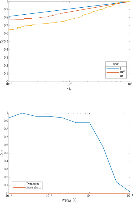
Figure 3: HMM glitch detector performance as a function of measurement uncertainty $\sigma_{\rm TOA}$. (Top panel.) ROC curve ($P_{\rm d}$ versus $P_{\rm fa}$) for three values of $\kappa/\kappa^{\ast}$ in the range $1\leq\kappa/\kappa^{\ast}\leq 10$, with $\kappa^{\ast}$ adjusted as a function of $\sigma_{\rm TOA}$ according to the recipe in Appendix C. (Bottom panel.) Detection probability $P_{\rm d}$ (blue curve) and false alarm probability $P_{\rm fa}$ (red curve, obscured by horizontal axis) versus $\sigma_{\rm TOA}$ (units: s), with the Bayes factor threshold kept at $10^{1/2}$ to give $P_{\rm fa}\approx 10^{-2}$ on average across the plotted range. Parameters: as in penultimate (typical) column in Table 1, except with $10^{-6}\leq\sigma_{\rm TOA}/(1\,{\rm s})\leq 10^{-3}$. Realizations: $1.5\times 10^{3}$ per ROC curve.

Quantity	Symbol	Units	Min	Typical	Max
Noise
Timing noise amplitude	$\sigma_{\rm TN}$	${\rm Hz\,s^{-1/2}}$	$10^{-15}$	$10^{-13}$	$10^{-11}$
TOA measurement uncertainty	$\sigma_{\rm TOA}$	${\rm s}$	$10^{-6}$	$10^{-5}$	$10^{-3}$
Scheduling
Mean waiting time	$\langle x_{n}\rangle$	d	$10^{-2}$	$13$	116
Number of sessions	—	—	5	51	$10^{2}$
Secular spin down
Frequency	$f_{\rm LS}$	${\rm Hz}$	$10^{0}$	5.435	$10^{2}$
Frequency derivative	$-\dot{f}_{\rm LS}$	${\rm Hz\,s^{-1}}$	$10^{-15}$	$10^{-15}$	$10^{-11}$
Glitch
Permanent frequency jump	$\Delta f_{\rm p}$	${\rm Hz}$	$10^{-10}$	$10^{-8}$	$10^{-7}$
Transient frequency jump	$\Delta f_{1}$	${\rm Hz}$	0	0	$10^{-8}$
Recovery time-scale	$\tau$	${\rm s}$	$10^{3}$	$10^{10}$	$10^{10}$
Permanent frequency derivative jump	$\Delta\dot{f}_{\rm p}$	${\rm Hz\,s^{-1}}$	$-10^{-12}$	$10^{-15}$	$10^{-15}$

Table 1: Parameters used to generate synthetic data to test the HMM, classified as astrophysical and measurement noise, scheduling of observations, secular spin down, and glitch parameters.

The HMM also contends with astrophysical timing noise. An important practical issue is how to select the HMM parameter $\sigma$ for a particular astrophysical target. Again, there is no unique prescription, and the final conclusions concerning glitch detection are conditional on the choice made. A useful rule of thumb is to match the root mean square phase residual $\langle\delta\phi(t_{n})^{2}\rangle^{1/2}$ accumulated by the random walk in the HMM, derived by integrating (9), with the phase residual accumulated by the timing noise in the pulsar, derived by integrating (20) and (21). The latter quantities are of order $\sigma\langle x_{n}\rangle^{5/2}$ and $\sigma_{\rm TN}\langle x_{n}\rangle^{3/2}$ respectively when integrated over the mean TOA gap, $\langle x_{n}\rangle$, which implies $\sigma\approx\langle x_{n}\rangle^{-1}\sigma_{\rm TN}=\sigma^{\ast}$. In practice $\langle x_{n}\rangle$ is dominated by the TOA intervals between rather than within observation sessions.

Figure 4 illustrates how the HMM’s performance varies, as $\sigma$ moves away from $\sigma^{\ast}$. The top panel displays five ROC curves for $10^{-1}\leq\sigma/\sigma^{\ast}\leq 10^{1}$. For $\sigma=\sigma^{\ast}$, we obtain $P_{\rm d}\geq 0.87$ for $P_{\rm fa}\geq 10^{-2}$ and $P_{\rm d}\geq 0.95$ for $P_{\rm fa}\geq 10^{-1}$. The results do not change much near the optimum, with $P_{\rm d}$ changing by $\lesssim 0.1$ over the range $10^{-1}\leq\sigma/\sigma^{\ast}\leq 10^{1}$ for $P_{\rm fa}\geq 10^{-2}$. The bottom panel in Figure 4 summarizes the results in practical, observation-ready terms. Adjusting $\sigma=\sigma^{\ast}$ as a function of $\sigma_{\rm TN}$ and $\langle x_{n}\rangle$ as in the previous paragraph, we find that the detection probability stays roughly constant, as $\sigma_{\rm TN}$ increases, with $P_{\rm d}\gtrsim 0.9$ (and $P_{\rm fa}\approx 10^{-2}$) for $\sigma_{\rm TN}\leq 10^{-12}(\Delta f_{\rm p}/10^{-8}\,{\rm Hz})\,{\rm Hz\,s^{-1/2}}$. We also find that $P_{\rm fa}$ rises steeply for $\sigma_{\rm TN}\gtrsim 10^{-12}(\Delta f_{\rm p}/10^{-8}\,{\rm Hz})\,{\rm Hz\,s^{-1/2}}$, as the HMM misinterprets strong timing noise as glitches. For reference, observations yield $10^{-15}\lesssim\sigma_{\rm TN}/(1\,{\rm Hz\,s^{-1/2}})\lesssim 10^{-11}$ typically for nonrecycled pulsars; for example, PSR J0534$+$2200 has $\sigma_{\rm TN}^{2}=6\times 10^{-23}\,{\rm Hz^{2}\,s^{-1}}$ (Cordes & Helfand, 1980). Therefore, even at the upper end of the measured $\sigma_{\rm TN}$ range, the HMM can detect glitches with $\Delta f_{\rm p}\gtrsim 10^{-7}\,{\rm Hz}$. Note that timing noise is red over long time-scales but approximately white over $\langle x_{n}\rangle$ in most observations. Care must be exercised when estimating $\sigma_{\rm TOA}$ and $\sigma_{\rm TN}$ indirectly from tempo2 residuals, because the Taylor expansion phase model correlates $\sigma_{\rm TOA}$ and $\sigma_{\rm TN}$ in a complicated way.

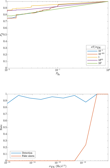
Figure 4: HMM glitch detector performance as a function of HMM noise parameter $\sigma$ and timing noise amplitude $\sigma_{\rm TN}$. (Top panel.) ROC curve ($P_{\rm d}$ versus $P_{\rm fa}$) for five values of $\sigma/\sigma^{\ast}$ in the range $10^{-1}\leq\sigma/\sigma^{\ast}\leq 10^{1}$, with $\sigma^{\ast}$ set according to the recipe in §6.1 as a function of $\sigma_{\rm TN}$ and $\langle x_{n}\rangle$. (Bottom panel.) Detection probability $P_{\rm d}$ (blue curve) and false alarm probability $P_{\rm fa}$ (red curve) versus $\sigma_{\rm TN}$ (units: ${\rm Hz\,s^{-1/2}}$), with the Bayes factor threshold held at $10^{1/2}$. The curves are restricted to $\sigma_{\rm TN}\leq 3\times 10^{-12}\,{\rm Hz\,s^{-1/2}}$ by the phase wandering mismatch described in §6.1. Parameters: as in Figure 3, except with $10^{-15}\leq\sigma_{\rm TN}/(1\,{\rm Hz\,s^{-1/2}})\leq 10^{-11}$. Realizations: $1.5\times 10^{3}$ per ROC curve.

In practice the rule of thumb $\sigma\approx\langle x_{n}\rangle^{-1}\sigma_{\rm TN}$ is modified by two factors: binning, and the functional form of the spin wandering. Binning errors in $\dot{f}$ impel $f(t)$ to drift. By setting $\sigma$ high enough to accommodate the drift in the transition probability, we ensure that the HMM self-corrects via the timing noise channel. The frequency residuals generated by $\dot{f}$ binning and timing noise are of order $\eta_{\dot{f}}\langle x_{n}\rangle$ and $\sigma\langle x_{n}\rangle^{3/2}$ respectively when integrated over the mean TOA gap, where $\eta_{\dot{f}}$ is the grid spacing in $\dot{f}$, implying $\sigma\geq\sigma_{\rm min}=\langle x_{n}\rangle^{-1/2}\eta_{\dot{f}}$ and hence $\sigma^{\ast}=\max(\sigma_{\rm min},\langle x_{n}\rangle^{-1}\sigma_{\rm TN})$. Additionally, the HMM is sensitive to the mismatch in phase wandering between the data (e.g. white noise in $\dot{f}$; see §5) and the transition probabilities (white noise in $\ddot{f}$; see §3.4). The mean square phase residuals arising from the two processes are given by $\sigma_{\rm TN}^{2}x_{n}^{3}$ and $\sigma^{2}x_{n}^{5}$ respectively when integrated over a specific TOA gap $x_{n}$. Substituting the rule of thumb $\sigma\approx\langle x_{n}\rangle^{-1}\sigma_{\rm TN}$, we calculate the frequency mismatch to be $\approx(\langle x_{n}\rangle^{-1}x_{n}-1)x_{n}^{1/2}\sigma_{\rm TN}$, which exceeds the frequency bin size $\eta_{f}$ for certain combinations of $x_{n}$, $\langle x_{n}\rangle$, and $\sigma_{\rm TN}$. For the parameters in the penultimate column of Table 1, with $\eta_{f}=6\times 10^{-10}\,{\rm Hz}$, the effect becomes significant for $\sigma_{\rm TN}\gtrsim 3\times 10^{-12}\,{\rm Hz\,s^{-1/2}}$, which corresponds to the cut-off in the curves in the bottom panel of Figure 4.

6.2 Secular spin down

Glitch detection is fundamentally an exercise in tracking fluctuations around the secular spin-down trend and distinguishing statistically between a continuous random walk (timing noise) and discontinuous jumps (glitches). One therefore expects the HMM’s performance to be approximately independent of the secular trend itself, i.e. $f_{\rm LS}$ and $\dot{f}_{\rm LS}$, as long as $\kappa\propto(\sigma_{\rm TOA}f_{\rm LS})^{-2}$ is held fixed, while the spin-down parameters vary. Figure 5 confirms that $P_{\rm d}$ stays approximately constant for $1\leq f_{\rm LS}/(1\,{\rm Hz})\lesssim 20$ and drops away for $f_{\rm LS}\gtrsim 20\,{\rm Hz}$ for the parameters in Table 1, because $\kappa$ decreases with $f_{\rm LS}$, when $\sigma_{\rm TOA}$ is held fixed. The roll-over shifts right, as $\sigma_{\rm TOA}$ decreases, and depends on $x_{n}$, $\eta_{f}$, and $\eta_{\dot{f}}$; there is nothing unique about $f_{\rm LS}\gtrsim 20\,{\rm Hz}$. Figure 5 also confirms that $P_{\rm d}\geq 0.9$ stays approximately constant across the plotted range $10^{-15}\leq\dot{f}_{\rm LS}/(1\,{\rm Hz\,s^{-1}})\leq 10^{-11}$, with $P_{\rm fa}\approx 10^{-2}$. Trials indicate that, for certain parameter combinations, $\sigma_{\rm TOA}$ is effectively underestimated when interpreted according to (8), leading to high $K_{1}(k)$ values and false alarms. As a precaution, we correct this behavior by taking $\sigma_{\rm TOA}$ to be $\approx 5$ times the fiducial tempo2 value. The correction factor is set empirically; it cannot be predicted analytically at present. It is conservative, as it reduces $P_{\rm d}$ marginally (by $\lesssim 10\%$) while nullifying the spike in $P_{\rm fa}$.

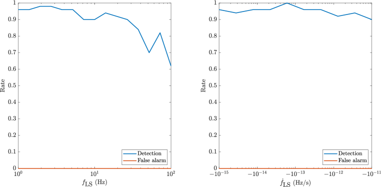
Figure 5: Detection probability (blue curve) and false alarm probability (red curve) versus secular spin-down parameters: $f_{\rm LS}$ (in ${\rm Hz}$) (left panel) and $\dot{f}_{\rm LS}$ (in ${\rm Hz\,s^{-1}}$) (right panel). Other parameters: see penultimate (typical) column in Table 1.

6.3 Glitch parameters

The size of the smallest glitch detectable by the HMM is governed chiefly by the user-selected probabilities $P_{\rm fa}$ and $P_{\rm d}$. In general, the permanent jump $\Delta f_{\rm p}$ is partially covariant with other glitch parameters (e.g. $\Delta\dot{f}_{\rm p}$, $\Delta f_{1}$, and $\tau$) as well as the non-glitch parameters discussed in §6.1–§6.2. However, we find that $\Delta f_{\rm p}$ affects $P_{\rm d}$ more strongly than the other parameters. Figure 6 illustrates this behavior. The top left panel shows that $P_{\rm d}$ rises steeply to $P_{\rm d}\geq 0.9$ for $\Delta f_{\rm p}\geq 8\times 10^{-9}\,{\rm Hz}$ and the parameters in the penultimate column of Table 1. The top right panel shows that $P_{\rm d}$ is roughly independent of $\Delta\dot{f}_{\rm p}$ in the range $-10^{-12}\leq\Delta\dot{f}_{\rm p}/(1\,{\rm Hz\,s^{-1}})\leq 10^{-15}$, where $\Delta\dot{f}_{\rm p}$ values of both signs are tested.

The bottom panels in Figure 6 illustrate how the HMM’s performance depends on the form and duration of the glitch recovery. In the bottom left panel, we observe that $P_{\rm d}$ rises to $P_{\rm d}\geq 0.5$ for $\tau\geq 2\times 10^{6}\,{\rm s}$, i.e. a glitch with a slower recovery is easier to detect. The plotted example involves a substantial transient component $\Delta f_{1}=\Delta f_{\rm p}$, which explains why $P_{\rm d}$ depends on $\tau$. The phase deviation produced by $\Delta f_{1}$ relative to the glitchless model builds up during the recovery and asymptotes to a constant value $\approx\tau\Delta f_{1}$, unlike the permanent component, whose phase deviation grows indefinitely as $\approx t\Delta f_{\rm p}$. The bottom right panel graphs $P_{\rm d}$ as a function of the transient fraction, $\Delta f_{1}/(\Delta f_{1}+\Delta f_{\rm p})$, holding $\Delta f_{1}+\Delta f_{\rm p}$ and $\tau$ fixed. We find $P_{\rm d}\leq 0.5$ for $\Delta f_{1}\gtrsim 0.6(\Delta f_{1}+\Delta f_{\rm p})$. That is, when the permanent fraction drops below some value, which depends on $\tau$, the glitch ceases to be detectable, if the transient component cannot be detected in its own right, i.e. if $\tau\Delta f_{1}$ is too low. Conversely, if $\Delta f_{\rm p}$ is large enough, the phase deviation crosses the detection threshold eventually, irrespective of $\Delta f_{1}$ and $\tau$.

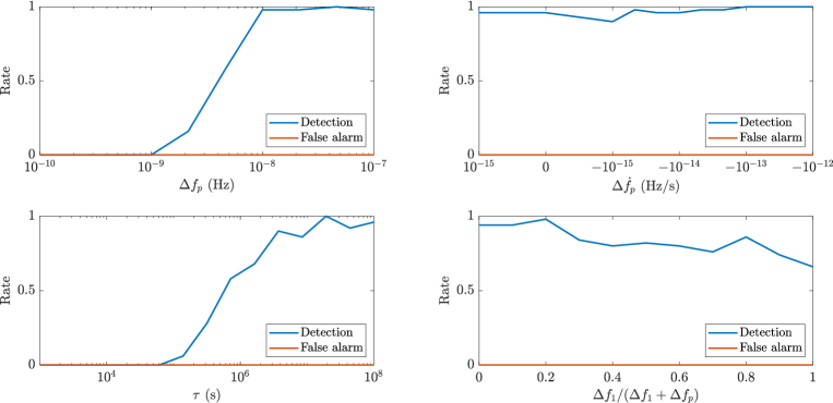
Figure 6: Detection probability (blue curve) and false alarm probability (red curve) versus glitch parameters: $\Delta f_{\rm p}$ (in ${\rm Hz}$) (top left panel), $\Delta\dot{f}_{\rm p}$ (in ${\rm Hz\,s^{-1}}$) (top right panel), $\tau$ (in ${\rm s}$) (bottom left panel), and recovery fraction $\Delta f_{1}/(\Delta f_{\rm p}+\Delta f_{1})$ (bottom right panel). Glitch parameters: $\Delta f_{1}=\Delta f_{\rm p}=5\times 10^{-9}\,{\rm Hz}$ (bottom left panel); $\Delta f_{1}+\Delta f_{\rm p}=1\times 10^{-8}\,{\rm Hz}$, $\tau=1\times 10^{5}\,{\rm s}$ (bottom right panel). Other parameters: see penultimate (typical) column in Table 1.

7 Representative worked example: PSR J0835$-$4510

The tests in this method paper are restricted deliberately to synthetic data, in order to quantify the performance of the HMM under controlled conditions. We look forward to applying the HMM to real, astrophysical data in the near future. As a foretaste, we analyse a publicly available subset of 490 TOAs from the regularly timed object PSR J0835$-$4510 from MJD 57427 to MJD 57810 (Sarkissian et al., 2017a, b). The data are preprocessed to cull the closest spaced TOAs (with $x_{n}\leq 8.9\times 10^{4}\,{\rm s}$ for definiteness), as these TOA clusters exhibit excess white noise in tempo2. Results are presented below for the preprocessed data, comprising $N_{T}=212$ TOAs, after checking for consistency against the 490 original TOAs.

7.1 2016 December 12 glitch

The results of applying the HMM to PSR J0835$-$4510 are presented in Figure 7. The first row displays the phase residuals arising from traditional tempo2 fits to the data. In the left panel, where the ephemeris does not incorporate a glitch, the phase wraps violently beyond the glitch epoch. In the right panel, where the ephemeris does incorporate a glitch, the phase wraps more slowly, because we do not correct for the quasiexponential post-glitch recovery in this panel. [The correction is performed by Sarkissian et al. (2017a) and Sarkissian et al. (2017b).] The second row of the figure displays the logarithm of the Bayes factor, $K_{1}(k)=\Pr[O_{1:N_{T}}|M_{1}(k)]/\Pr(O_{1:N_{T}}|M_{0})$, for $1\leq k\leq N_{T}$ and $\sigma=5\times 10^{-16}\,{\rm Hz\,s^{-3/2}}$. The value of $\sigma$ is estimated from the tempo2 residuals and the gridding bound $\sigma\geq 1.3\times 10^{-16}$ [dominated by $\eta_{\dot{f}}$ in (C3)] plus a conservative safety factor. The one-glitch model $M_{1}(173)$ is preferred strongly over $M_{0}$ and all $M_{1}(k)$ with $k\neq 173$ ($k\neq 383$ before preprocessing). The HMM glitch epoch, $T=57734.54\,{\rm MJD}$, approaches that obtained by traditional methods, which yield $T=57734.4855(4)\,{\rm MJD}$ (Palfreyman, 2016; Sarkissian et al., 2017b; Ashton et al., 2019). The maximum Bayes factor is huge, with $\ln K_{1}(173)=1.1\times 10^{3}$, a testament to the discriminating power of the HMM. The third row displays $\hat{f}(t)$ versus $t$, inferred using the HMM forward-backward algorithm, for $M_{0}$ (left panel) and $M_{1}(173)$ (right panel). The frequency step in the right panel is clearly visible. The fourth row displays the associated phase residuals, which wrap violently for $M_{0}$ at $t>T$ while remaining roughly constant for $M_{1}(173)$. The results confirm, that $M_{1}(173)$ offers a good description of the 2016 December 12 event despite modeling it as a step for simplicity, without a post-glitch recovery.

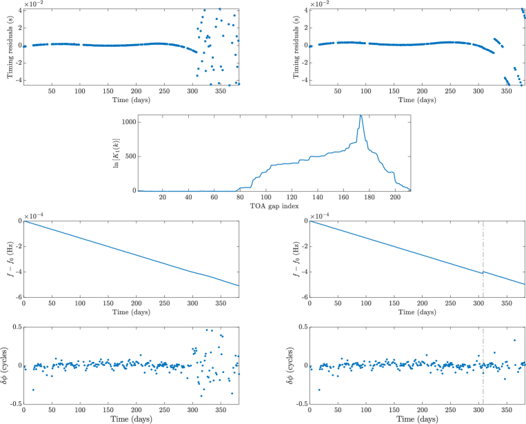
Figure 7: HMM analysis of $212$ TOAs measured for PSR J0835$-$4510 from MJD 57427 to MJD 57810 (Sarkissian et al., 2017a, b). (First row.) Phase residuals $\delta\phi(t_{n})$ versus TOA $t_{n}$ computed with tempo2 for no-glitch (left panel) and one-glitch (right panel) models, with $T=57734.54\,{\rm MJD}$, $\Delta f_{\rm p}=1.596\times 10^{-5}\,{\rm Hz}$, $\Delta\dot{f}_{\rm p}=-4.4\times 10^{-13}\,{\rm Hz\,s^{-1}}$ in the one-glitch model. (Second row.) Logarithm of the Bayes factor, $K_{1}(k)$, versus TOA index, $k$, computed with the HMM using $\sigma=5\times 10^{-16}\,{\rm Hz\,s^{-3/2}}$ and the DOI $f_{\rm LS}=11.1868550196\,{\rm Hz}$, $\dot{f}_{\rm LS}=1.55886\times 10^{-11}\,{\rm Hz\,s^{-1}}$, $-5.5\times 10^{-4}\leq(f-f_{\rm LS})/(1\,{\rm Hz})\leq 1\times 10^{-5}$, $-2\times 10^{-12}\leq(\dot{f}-\dot{f}_{\rm LS})/(1\,{\rm Hz\,s^{-1}})\leq 2\times 10^{-12}$, $\eta_{f}=5.606\times 10^{-7}\,{\rm Hz}$ ($10^{3}$ bins) and $\eta_{\dot{f}}=4\times 10^{-14}\,{\rm Hz\,s^{-1}}$ (101 bins). (Third row.) Recovered frequency $f(t_{n})$ versus TOA $t_{n}$ for the no-glitch (left panel) and one-glitch (right panel) HMM models $M_{0}$ and $M_{1}$. The vertical dashed line marks the glitch. (Fourth row.) Unsummed per-gap phase residuals $\delta\phi(t_{n})$ versus TOA $t_{n}$ for the HMM forward-backward sequences in the third row.

In order to check the robustness of the conclusion, that $M_{1}(173)$ is the preferred model, we subdivide the data set into halves and quarters and plot $K_{1}(k)$ versus $k$ in Figure 8. The results for each subdivision are color-coded according to the legend. No matter how the data are subdivided, the conclusion is the same: $M_{1}(173)$ is strongly preferred over $M_{0}$ and $M_{1}(k)$ with $k\neq 173$ in the data segments that include $t_{173}$, and $M_{1}(173)$ is not rivaled by a better alternative in the data segments that do not include $t_{173}$.

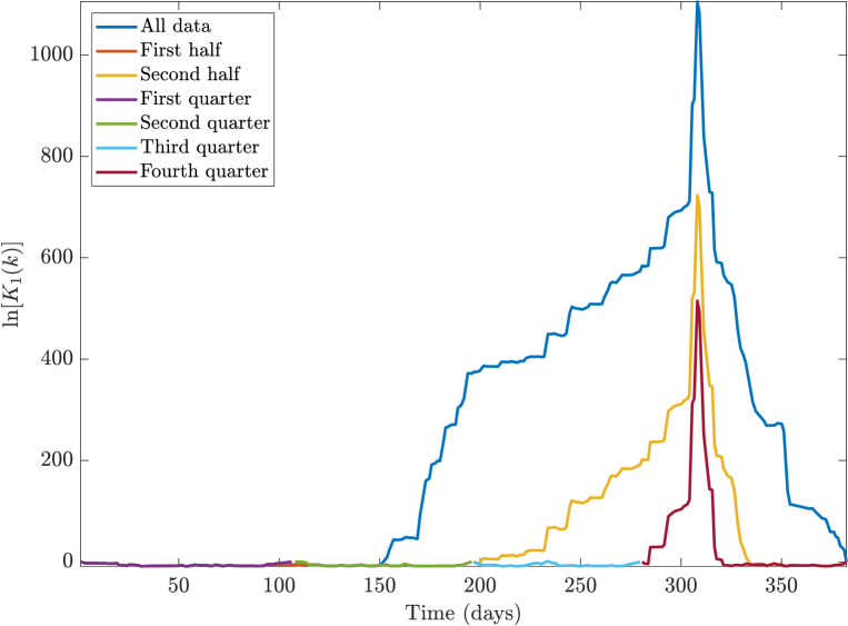
Figure 8: Logarithm of the Bayes factor, $K_{1}(k)$, versus TOA index, $k$, for PSR J0835$-$4510 from MJD 57427 to MJD 57810, computed with the same HMM parameters as in Figure 7, but with the data segmented into halves (red and yellow curves) and quarters (purple, green, light blue, and brown curves). The blue curve, incorporating all the data, is copied from Figure 7 for comparison.

How does the recovered ephemeris compare with the traditional timing solution, now that the glitch is detected? Figure 9 presents the evolution of the posterior PDF $\gamma_{q_{i}}(t_{n})$ before and after the glitch. The first and second rows display contours of $\gamma_{q_{i}}(t_{n})$ marginalized over $\dot{f}$ and $f$ respectively, graphed as functions of $t_{n}$, together with the point-wise optimal sequences $\hat{f}(t_{n})$ and $\hat{\dot{f}}(t_{n})$ respectively. Both marginalized posteriors are strongly and singly peaked around the optimal sequences. The jump in $\hat{f}(t_{n})$ is visible in the top row. The third and fourth rows display orthogonal cross-sections taken through the posterior PDF just before ($t_{172}$; third row) and after ($t_{174}$; fourth row) the glitch. In the left column, where $\gamma_{q_{i}}(t_{n})$ is marginalized over $\dot{f}$, there is an upward shift in frequency, with $\Delta f_{\rm p}=\hat{f}(t_{174})-\hat{f}(t_{172})=1.596\times 10^{-5}\,{\rm Hz}$. The cross-sections are narrow, spanning $\lesssim 4$ bins before and after the glitch. In the right column, where $\gamma_{q_{i}}(t_{n})$ is marginalized over $f$, there is a downward shift in frequency derivative, with $\Delta\dot{f}_{\rm p}=\hat{\dot{f}}(t_{174})-\hat{\dot{f}}(t_{172})=-4.4\times 10^{-13}\,{\rm Hz\,s^{-1}}$. The shift is significant in the sense that it exceeds the dispersion, which actually decreases during the event (FWHM $\lesssim 8$ bins before, cf. $\lesssim 2$ bins after). The inferred jumps agree with traditional pulsar timing methods, which give $\Delta f_{\rm p}=1.6044(2)\times 10^{-5}\,{\rm Hz}$ and $\Delta\dot{f}_{\rm p}=-1.21(3)\times 10^{-13}\,{\rm Hz\,s^{-1}}$ (Palfreyman, 2016; Sarkissian et al., 2017b), after allowing for the fact that the HMM transition probabilities do not include the post-glitch relaxation with $\tau=0.96(17)\,{\rm d}$. (Including the relaxation is straightforward but lies outside the scope of this paper.) All in all, the optimal sequence stands out clearly above its nearest competitors.

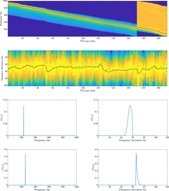
Figure 9: Evolution of the posterior PDF $\gamma_{q_{i}}(t_{n})$ defined by (A13), for PSR J0835$-$4510 from MJD 57427 to MJD 57810, in the vicinity of the optimal values $\hat{f}(t_{n})$ and $\hat{\dot{f}}(t_{n})$. (First row.) Contours of $\gamma_{q_{i}}(t_{n})$ marginalized over $\dot{f}$ (arbitrary color scale; yellow high, blue low) versus TOA index $n$, with the point-wise optimal (forward-backward) state sequence overplotted (red curve). (Second row.) Contours of $\gamma_{q_{i}}(t_{n})$ marginalized over $f$ versus TOA index $n$. (Third row.) Cross-section of $\gamma_{q_{i}}(t_{n})$ marginalized over $\dot{f}$ (left column) and $f$ (right column) at $n=172$, i.e. at the TOA preceding the recovered glitch. The horizontal axes display numbers of bins. (Fourth row.) Cross-section of $\gamma_{q_{i}}(t_{n})$ marginalized over $\dot{f}$ (left column) and $f$ (right column) at $n=174$, i.e. at the TOA following the recovered glitch. Parameters: see Figure 7.

7.2 Additional glitches

A systematic search for multiple glitches lies outside the scope of this paper. Nonetheless, again as a foretaste of what is feasible, we search for a second glitch in PSR J0835$-$4510 from MJD 57427 to MJD 57810 by applying the greedy hierarchical algorithm introduced in §4.2 (Suvorova et al., 2018). The analysis is presented in Appendix H. We conclude that no statistically significant second event exists, in accord with previous analyses (Sarkissian et al., 2017a, b).

We look forward to applying the HMM to more real data sets. In particular, a fuller search for glitches in PSR J0835$-$4510 over several decades of continuous monitoring using the greedy hierarchical algorithm in §4.2 will be undertaken in future work; the relevant data are not currently at our disposal. If additional events are found, they can be cross-checked in many ways. One can apply the HMM to data taken with a different telecope, e.g. the higher cadence Mount Pleasant Radio Observatory for PSR J0835$-$4510 (Palfreyman et al., 2018), just as when checking the output of traditional timing methods. The Mount Pleasant data were analysed recently by Bayesian methods to study the pulse-to-pulse dynamics of the 2016 December 12 glitch (Ashton et al., 2019). One can also test, how the Bayes factor changes, as one tunes HMM parameters like $\kappa$, $\sigma$, and $P_{\rm fa}$; see §6.1 for details. It is faster to do such tests systematically with the HMM than with traditional timing methods.

8 Conclusion

In this method paper, a new, systematic scheme is presented for detecting pulsar glitches given a sequence of standard TOAs. The scheme is structured around a HMM, which tracks the evolution of the pulse frequency and its first time derivative on long (electromagnetic spin down), intermediate (timing noise), and short (glitches) time-scales. The emission probability of the HMM obeys a von Mises distribution. The transition probability obeys a Gaussian distribution derived from the Fokker-Planck equation for an unbiased Wiener process. The HMM forward algorithm is used to compute and compare the Bayesian evidence for models with and without glitches. Once the preferred model is selected, the HMM forward-backward algorithm is used to compute the associated, point-wise optimal ephemeris, composed of the most probable hidden state $\hat{q}(t_{n})$ at each $t_{n}$ given all the observations $O_{1:N_{T}}$. The algorithm and testing procedure are documented in Appendices A–H for the sake of reproducibility.

Monte Carlo simulations demonstrate that the HMM detects glitches accurately in synthetic data for a range of realistic intrinsic and measurement noises ($\sigma_{\rm TN}$, $\sigma_{\rm TOA}$; see §6.1), secular spin-down parameters ($f_{\rm LS}$, $\dot{f}_{\rm LS}$; see §6.2), glitch parameters ($\Delta f_{\rm p}$, $\Delta\dot{f}_{\rm p}$, $\Delta f_{1}$, $\tau$; see §6.3), and observational schedules ($\langle x_{n}\rangle$, $N_{T}$; see Appendix G). The performance of the HMM, in particular the trade off between $P_{\rm fa}$ and $P_{\rm d}$, is quantified systematically in terms of ROC curves constructed as functions of the above parameters. Success is achieved, even though (i) the HMM approximates glitches as instantaneous steps in $f$ and $\dot{f}$ without any post-glitch recovery, and (ii) the HMM models timing noise as white noise in the torque derivative (and hence red noise in the filtered torque), an approximation which applies to some but not all pulsars (Cordes, 1980; Cordes & Downs, 1985) and is violated deliberately when generating the synthetic data in this paper in order to challenge the robustness of the HMM. Several trends of practical utility are identified. (i) The HMM performs stably, neither overestimating nor underestimating the number of glitches, for $\sigma\approx\langle x_{n}\rangle^{-1}\sigma_{\rm TN}$, with $\sigma_{\rm TN}$ computed from the tempo2 phase residuals, as described in §6.1. (ii) In order to detect a glitch of size $\Delta f_{\rm p}$, it is recommended to schedule observations with $\langle x_{n}\rangle^{1/2}\lesssim\sigma_{\rm TN}^{-1}\Delta f_{\rm p}$, independent of the number of TOAs per continuous observing session. Roughly equal spacing is preferable, as false alarms occur more commonly adjacent to longer TOA gaps. (iii) Performance is essentially unaffected by $\dot{f}_{\rm LS}$ and depends roughly on the product $\sigma_{\rm TOA}f_{\rm LS}$. (iv) The size of the smallest detectable glitch is governed mainly by $\Delta f_{\rm p}$ and depends weakly on $\tau$, when the phase deviation produced by $\Delta f_{\rm p}$ exceeds that produced by the transient ($\approx\tau\Delta f_{1}$). (v) Recipes for setting the DOI and grid resolution are set out in Appendix C.

The performance tests in this paper are restricted deliberately to synthetic data in order to establish performance bounds systematically under controlled conditions. Nevertheless, as a foretaste of what can be achieved with astronomical data, we also apply the HMM to 490 publicly available TOAs from PSR J0835$-$4510, covering the interval from MJD 57427 to MJD 57810 (Sarkissian et al., 2017a, b). We confirm the existence of the large glitch on 2016 December 12, with log Bayes factor $\approx 1.1\times 10^{3}$, and rule out with high statistical confidence the existence of a second glitch during the same interval. The inferred ephemeris, including $\Delta f_{\rm p}$ and $\Delta\dot{f}_{\rm p}$, agrees with that yielded by traditional timing methods, after allowing for the fact that the introductory HMM in this paper does not include post-glitch recoveries. We look forward to applying the HMM to other pulsars, both to detect glitches and to improve the sensitivity of nanohertz gravitational wave searches with pulsar timing arrays (Lentati et al., 2015; Shannon et al., 2015; Arzoumanian et al., 2016; Hobbs & Dai, 2017).

In closing, we reaffirm that the HMM scheme developed in this paper complements — but does not replace — traditional glitch finding approaches based on least-squares fitting of a Taylor-expanded phase model plus glitch template. Indeed, the HMM ingests standard TOAs and leverages the outputs of existing software [e.g. $f_{\rm LS}$, $\dot{f}_{\rm LS}$, and phase residuals $\delta\phi(t_{n})$ from tempo2] to demarcate its state space (DOI). It complements existing Bayesian approaches, e.g. temponest (Lentati et al., 2014; Shannon et al., 2016; Lower et al., 2018), by tracking the observed spin wandering explicitly, as a specific realization of a discrete-time Markov chain, instead of estimating its ensemble statistics (e.g. power spectral density). Every approach has advantages and disadvantages. The HMM is unsupervised, so its performance bounds (e.g. $P_{\rm fa}$, $P_{\rm d}$) can be computed efficiently. It is fast, requiring $\sim 10^{12}$ floating point operations ($\sim 0.1$ CPU hours) per pulsar per year of observations. It discriminates accurately between spin wandering and glitches by tracking both phenomena explicitly with a Markov chain. On the other hand, when spin wandering and glitches are negligible, the HMM is superfluous. Pulse domain methods ultimately promise the best sensitivity but they expend a lot of computational effort correcting for random pulse-to-pulse profile variations and do not ingest standard TOAs. They may be strongest when combined with an HMM similar to the one described here. If the problem allows, it is wise to apply several methods simultaneously. There is no purely objective answer to the question of whether or not a data set contains a glitch. The question is fundamentally statistical and can only be answered in the context of a user-selected false alarm probability. The results in this paper show concretely and systematically how to define, compute, and set $P_{\rm fa}$ for the HMM.

Appendix A Solving the HMM

Let $M=\{A_{q_{j}q_{i}},L_{o(t_{n})q_{i}},\Pi_{q_{i}}\}$ be a HMM with transition probability $A_{q_{j}q_{i}}$, emission probability $L_{o(t_{n})q_{i}}$, and prior probability $\Pi_{q_{i}}$ defined according to (1), (2), and (4) respectively. Let $Q_{m:n}=\{q(t_{m}),\dots,q(t_{n})\}$ and $O_{m:n}=\{o(t_{m}),\dots,o(t_{n})\}$ denote arbitrary, partial sequences of hidden and observed states respectively, with $1\leq m\leq n\leq N_{T}$. In this appendix, we present efficient numerical algorithms, which exploit recursion to solve the two fundamental HMM problems below.

1. What is the Bayesian evidence $\Pr(O_{1:N_{T}}|M)$ for the model $M$, given the full observed sequence, $O_{1:N_{T}}$? This question reduces to calculating

   $$\Pr(O_{1:N_{T}}|M) = \sum_{Q_{1:N_{T}}}\Pr(O_{1:N_{T}}|Q_{1:N_{T}},M)\Pr(Q_{1:N_{T}},M)$$ (A1)

   $$= \sum_{Q_{1:N_{T}}}\Pi_{q(t_{1})}L_{o(t_{1})q(t_{1})}\prod_{n=2}^{N_{T}}A_{q(t_{n-1})q(t_{n})}L_{o(t_{n})q(t_{n})}~{}.$$ (A2)

2. What is the optimal hidden sequence given $M$ and $O_{1:N_{T}}$? This question reduces to calculating

   $$\hat{q}(t_{n}) = \underset{q(t_{n})}{\rm arg\,\,max\,\,}\sum_{Q_{1:n-1}}\Pi_{q(t_{1})}L_{o(t_{1})q(t_{1})}\prod_{m=2}^{n-1}A_{q(t_{m-1})q(t_{m})}L_{o(t_{m})q(t_{m})}$$ (A3)

   $$\times A_{q(t_{n-1})q(t_{n})}L_{o(t_{n})q(t_{n})}\sum_{Q_{n+1:N_{T}}}\prod_{m=n+1}^{N_{T}}A_{q(t_{m-1})q(t_{m})}L_{o(t_{m})q(t_{m})}$$

   for $2\leq n\leq N_{T}$ and a uniform prior, if one wishes to maximize $\Pr[q(t_{n})|O_{1:N_{T}},M]$ point-wise, or

   $$Q_{1:N_{T}}^{\ast}=\underset{Q_{1:N_{T}}}{\rm arg\,\,max\,\,}\Pi_{q(t_{1})}L_{o(t_{1})q(t_{1})}\prod_{n=2}^{N_{T}}A_{q(t_{n-1})q(t_{n})}L_{o(t_{n})q(t_{n})}~{},$$ (A4)

   if one wishes to maximize $\Pr(Q_{1:N_{T}}|O_{1:N_{T}})$ sequence-wise. The difference between options (A3) and (A4) is explained below.

The above problems are essential building blocks of the glitch-finding algorithm in §4. A third fundemantal problem — given $O_{1:N_{T}}$, what model $M$ maximizes the Bayesian evidence $\Pr(O_{1:N_{T}}|M)$? — amounts to learning the optimal model (here, the glitch dynamics) from the data. It is of great interest but lies outside the scope of this paper. The reader is referred to the excellent tutorial by Rabiner (1989) for a fuller treatment of the fundamental principles of HMMs.

A.1 Forward algorithm

It may seem that evaluating the sum (A2) involves $\sim N_{T}N_{Q}^{N_{T}}$ floating point operations, because each term is a product of $2N_{T}$ factors, and there are $N_{Q}^{N_{T}}$ possible hidden sequences. Fortunately recursive filtering offers a more efficient approach.

Consider the forward variable

$$\alpha_{q_{i}}(t_{n})=\Pr[q(t_{n})=q_{i},O_{1:n}|M]~{},$$ (A5)

i.e. $\alpha_{q_{i}}(t_{n})$ equals the probability that one observes the partial data $O_{1:n}$ during the interval $t_{1}\leq t\leq t_{n}$, and the system occupies the state $q_{i}$ at time $t=t_{n}$. Notice that, at $t=t_{n}$, every one of the $N_{Q}$ hidden states is reached from the same $N_{Q}$ hidden states at $t=t_{n-1}$. Hence one can calculate (A2) by addressing every link in the trellis in Figure 10 once, instead of backtracking over every link multiple times while tracing all $N_{Q}^{N_{T}}$ hidden sequences separately. The following algorithm achieves this economy by storing the partial results at each forward step through the trellis (Rabiner, 1989; Quinn & Hannan, 2001).

1. Initialization. For $1\leq i\leq N_{Q}$, set

   $$\alpha_{q_{i}}(t_{1})=\Pi_{q_{i}}L_{o(t_{1})q_{i}}~{}.$$ (A6)

2. Induction. For $1\leq n\leq N_{T}-1$ and $1\leq i\leq N_{Q}$, compute the forward variable by summing over its values at the previous HMM step:

   $$\alpha_{q_{i}}(t_{n+1})=L_{o(t_{n+1})q_{i}}\sum_{j=1}^{N_{Q}}A_{q_{i}q_{j}}\alpha_{q_{j}}(t_{n})~{}.$$ (A7)

3. Termination. The Bayesian evidence is the sum of the forward variable over the final states, viz.

   $$\Pr(O_{1:N_{T}}|M)=\sum_{i=1}^{N_{Q}}\alpha_{q_{i}}(t_{N_{T}})~{}.$$ (A8)

The trellis contains $N_{Q}^{2}$ links per HMM transition, and there are $N_{T}-1$ transitions, so the computation involves $\sim N_{T}N_{Q}^{2}$ floating point operations in total, a large saving.

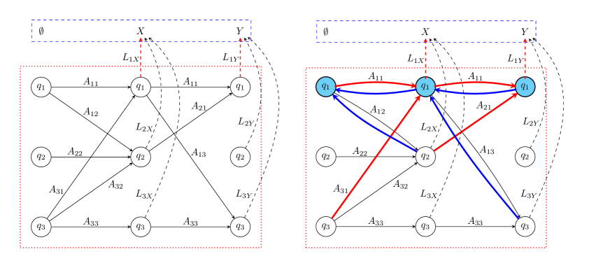
Figure 10: Schematic of the HMM trellis. (Left panel.) Subset of the links in the trellis. Every circle denotes a hidden state ($q_{1}$, $q_{2}$, $q_{3}$) at some time step (time increases to the right). The top rectangle contains the data ($X$, $Y$). Every unbroken arrow corresponds to a nonzero transition probability, e.g. $A_{12}$ is the probability of transitioning from $q_{1}$ to $q_{2}$. Every broken arrow corresponds to a nonzero emission probability, e.g. $L_{2Y}$ is the probability of observing the data $Y$ at the third time-step while occupying hidden state $q_{2}$. (Right panel.) Sample of the links that go into evaluating the induction step for $\gamma_{q_{1}}$ (circles shaded blue) for the forward variable [red arrows; equation (A7)] and the backward variable [blue arrows; equation (A11)].

A.2 Forward-backward algorithm

The maximization step in (A3) can be executed with the help of recursive smoothing, without comparing the $N_{Q}^{N_{T}}$ hidden sequences severally. This is achieved by introducing a backward variable, analogous to the forward variable above, and then maximizing the product of the forward and backward variables.

Consider the backward variable,

$$\beta_{q_{i}}(t_{n})=\Pr[O_{n+1:N_{T}}|q(t_{n})=q_{i},M]~{},$$ (A9)

i.e. $\beta_{q_{i}}(t_{n})$ equals the probability that one observes the partial data $O_{n+1:N_{T}}$ during the interval $t_{n+1}\leq t\leq N_{T}$, conditional on the system occupying the state $q_{i}$ at time $t=t_{n}$. Every one of the hidden states at $t=t_{n}$ connects to the same set of hidden states at $t=t_{n+1}$, so one can express $\beta_{q_{i}}(t_{n})$ inductively in terms of $\beta_{q_{1}}(t_{n+1}),\dots,\beta_{q_{N_{Q}}}(t_{n+1})$ by summing over the $N_{Q}$ possible transitions from $q_{i}(t_{n})$ to $q_{1}(t_{n+1}),\dots,q_{N_{Q}}(t_{n+1})$ (Rabiner, 1989).

1. Initialization. For $1\leq i\leq N_{Q}$, set

   $$\beta_{q_{i}}(t_{N_{T}})=1~{}.$$ (A10)

2. Induction. For $1\leq n\leq N_{T}-1$ and $1\leq i\leq N_{Q}$, compute the backward variable by summing over its values at the succeeding HMM step, starting from $n=N_{T}-1$ and stepping back to $n=1$.

   $$\beta_{q_{i}}(t_{n})=\sum_{j=1}^{N_{Q}}A_{q_{i}q_{j}}L_{o(t_{n+1})q_{j}}\beta_{q_{j}}(t_{n+1})~{}.$$ (A11)

The backward algorithm (A9)–(A11) entails $\sim N_{T}N_{Q}^{2}$ floating point operations like the forward algorithm.

We now ask what hidden state is most likely to be occupied at $t=t_{n}$, given the entire observed sequence $O_{1:N_{T}}$ and the model $M$. Define

$$\gamma_{q_{i}}(t_{n}) = \Pr[q(t_{n})=q_{i}|O_{1:N_{T}},M]$$ (A12)

$$= \left[\sum_{j=1}^{N_{Q}}\alpha_{q_{j}}(t_{n})\beta_{q_{j}}(t_{n})\right]^{-1}\alpha_{q_{i}}(t_{n})\beta_{q_{i}}(t_{n})~{},$$ (A13)

where (A13) follows from (A12), because the forward variable accounts for the hidden and observed sequences $Q_{1:n}$ and $O_{1:n}$ terminating at $q(t_{n})=q_{i}$, and the backward variable accounts for the hidden and observed sequences $Q_{n:N_{T}}$ and $O_{n:N_{T}}$ originating at $q(t_{n})=q_{i}$. Equation (A13) implies that the most likely state at each HMM step is given by

$$\hat{q}(t_{n})=\underset{1\leq i\leq N_{Q}}{\rm arg\,\,max\,\,}\gamma_{q_{i}}(t_{n})$$ (A14)

for $1\leq n\leq N_{T}$. The denominator of (A13) is a normalization factor which, for $t=N_{T}$, reduces to $\Pr(O_{1:N_{T}}|M)$ in (A2) via (A8) and (A10). It can be ignored when maximizing over $1\leq i\leq N_{Q}$. Equations (A5)–(A14) together constitute the HMM forward-backward algorithm. The algorithm entails $\sim N_{T}N_{Q}^{2}$ floating point operations, dominated by (A11)–(A13); the final step (A14) reduces to $\sim N_{T}\ln N_{Q}$ operations with binary maximization.

The above solution of the HMM optimization problem is not unique. It does maximize the number of most probable hidden states. On the other hand, there is no guarantee that the sequence generated thus is admissible, i.e. consistent with the transition probabilities. For example, if we have $A_{q_{j}q_{i}}=0$ for some $q_{j}$ and $q_{i}$, it may not be possible to connect the sequence $\{\hat{q}(t_{1}),\dots,\hat{q}(t_{N_{T}})\}$ generated by (A14). In this sense, $\{\hat{q}(t_{1}),\dots,\hat{q}(t_{N_{T}})\}$ differs subtly from $Q^{\ast}_{1:N_{T}}$ in (A4). The latter quantity is admissible by construction and maximizes the probability of the whole sequence rather than individual states along the sequence. In general, both approaches (and indeed others not discussed here) are valid. In this paper, we focus on $\{\hat{q}(t_{1}),\dots,\hat{q}(t_{N_{T}})\}$ for three reasons. First, we wish to maximize the number of most probable hidden states when generating an ephemeris. Second, we find by trial and error that inadmissibility arises rarely in the glitch-finding application. Third, we wish to know the shape of the joint PDF of $f(t_{n})$ and $\dot{f}(t_{n})$ at each $t_{n}$, in order to check how far the optimal sequence stands above its nearest competitors. This is done easily by plotting $\gamma_{q_{i}}(t_{n})$ versus $q_{i}$, whereas $Q^{\ast}_{1:N_{T}}$ gives the best sequence only. Traditional, frequentist pulsar timing methods involve a mixture of point-wise and sequence-wise optimization by minimizing the squares of the point-by-point phase residuals summed over the entire sequence.

A.3 Viterbi algorithm

For the sake of completeness, we outline an algorithm for calculating $Q^{\ast}_{1:N_{T}}$ in (A4). Known as the Viterbi algorithm, and based on dynamic programming methods, it exploits the property that any subsequence of the optimal sequence is itself optimal in order to prune the trellis of admissible sequences (Rabiner, 1989; Quinn & Hannan, 2001). The pseudocode below matches closely the notation adopted by Rabiner (1989) and in recent gravitational wave applications (Suvorova et al., 2016); cf. Bayley et al. (2019).

Consider the variable

$$\delta_{q_{i}}(t_{n}) = \max_{Q_{1:n-1}}\Pr[q(t_{n})=q_{i},Q_{1:n-1}|O_{1:n},M]~{},$$ (A15)

$$= L_{o(t_{n})q_{i}}\max_{q_{j}}A_{q_{i}q_{j}}\delta_{q_{j}}(t_{n-1})~{},$$ (A16)

which corresponds to the maximum probability, that the HMM terminates in the hidden state $q_{i}$ at $t=t_{n}$ given the partial observation sequence $O_{1:n}$. Let $\psi_{q_{i}}(t_{n})$ denote the hidden state at $t=t_{n-1}$ from which $q_{i}$ is reached at $t=t_{n}$, along the sequence that maximizes $\Pr[q(t_{n})=q_{i},Q_{1:n-1}|O_{1:n},M]$ in (A15), viz.

$$\psi_{q_{i}}(t_{n})=\underset{q_{j}}{\rm arg\,max\,}A_{q_{i}q_{j}}\delta_{q_{j}}(t_{n-1})~{}.$$ (A17)

The Viterbi algorithm evaluates $\delta_{q_{i}}(t_{n})$ and $\psi_{q_{i}}(t_{n})$ for all of the $N_{Q}N_{T}$ nodes in the trellis in Figure 10 and then backtracks to reconstruct $Q^{\ast}_{1:N_{T}}$. It resembles the forward algorithm, with the sum in (A7) replaced by the maximization steps in (A16) and (A17).

1. Initialization. For $1\leq i\leq N_{Q}$, set

   $$\delta_{q_{i}}(t_{1})=\Pi_{q_{i}}L_{o(t_{1})q_{i}}~{},$$ (A18)

   Note that $\psi_{q_{i}}(t_{1})$ is not initialized as it is never needed.

2. Forward recursion. For $2\leq n\leq N_{T}$ and $1\leq i\leq N_{Q}$, implement the induction step (A16) via

   $$\delta_{q_{i}}(t_{n})=L_{o(t_{n})q_{i}}\max_{1\leq j\leq N_{Q}}A_{q_{i}q_{j}}\delta_{q_{j}}(t_{n-1})$$ (A19)

   and

   $$\psi_{q_{i}}(t_{n})=\underset{1\leq j\leq N_{Q}}{\rm arg\,max\,}A_{q_{i}q_{j}}\delta_{q_{j}}(t_{n-1})~{}.$$ (A20)

3. Termination. Identify the state $q^{\ast}(t_{N_{T}})$, where the optimal sequence ends.

   $$\Pr(Q^{\ast}_{1:N_{T}}|O_{1:N_{T}},M)=\max_{1\leq j\leq N_{Q}}\delta_{q_{j}}(t_{N_{T}})$$ (A21)

   and

   $$q^{\ast}(t_{N_{T}})=\underset{1\leq j\leq N_{Q}}{\rm arg\,max\,}\delta_{q_{j}}(t_{N_{T}})~{}.$$ (A22)

4. Backward recursion. Backtrack through the trellis in Figure 10 to reconstruct the optimal sequence, guided by $\psi_{q_{j}}(t_{n})$. For $1\leq n\leq N_{T}-1$, compute

   $$q^{\ast}(t_{n})=\psi_{q^{\ast}(t_{n+1})}(t_{n+1})~{},$$ (A23)

   starting from $n=N_{T}-1$ and stepping back to $n=1$.

The algorithm involves $\sim N_{T}N_{Q}\ln N_{Q}$ floating point operations with binary maximization (Quinn & Hannan, 2001).

Appendix B Hidden state evolution via a Langevin equation

In this appendix we derive the transition probabilities in §3.4 self-consistently by solving a stochastic differential equation for $q(t)=[f(t),\dot{f}(t)]$ in the inter-step interval $t_{n-1}\leq t\leq t_{n}$. Although the system is measured at discrete instants $t_{n}$, its state evolves stochastically between the TOAs due to timing noise (Cordes, 1980). For now, we neglect the secular component of the torque derivative, $\langle\ddot{f}\rangle$, a good approximation provided that $x_{n}^{2}\lesssim 6f(t_{n})/|\ddot{f}(t_{n})|$ is satisfied; see §3.1. This leaves an approximately constant secular torque, which enters as an initial condition on $\dot{f}(t_{n-1})$, and a fluctuating torque derivative $\xi(t)$, which drives the Langevin equation,

$$\frac{d^{2}f}{dt^{2}}=\xi(t)~{},$$ (B1)

with white noise statistics,

$$\langle\xi(t)\rangle=0$$ (B2)

and

$$\langle\xi(t)\xi(t^{\prime})\rangle=\sigma^{2}\delta(t-t^{\prime})~{}.$$ (B3)

Angular brackets denote an ensemble average over noise realizations.

Unlike $\sigma_{\rm TOA}^{2}$, the variance $\sigma^{2}$ is not a measurement uncertainty. It is a mean-square measure of the amplitude of the process noise driven by the fluctuating torque derivative, which may arise physically from starquakes and superfluid vortex avalanches for example (Chugunov & Horowitz, 2010; Warszawski & Melatos, 2011; Haskell & Melatos, 2015). Its units are ${\rm Hz^{2}\,s^{-3}}$, cf. $\sigma_{\rm TOA}^{2}$, which has units of ${\rm s}^{2}$. Likewise, $\sigma^{2}$ is not the same as $\sigma_{\rm TN}^{2}$ in the synthetic data in §5, because $\sigma_{\rm TN}^{2}$ equals the variance in the autocorrelation function of the torque, not the torque derivative. White noise fluctuations in the torque derivative, as in (B1), are not necessarily physical; they are an artificial device to keep $A_{q_{j}q_{i}}$ finite. By contrast, a fluctuating torque gives $\langle\dot{f}(t)\dot{f}(t^{\prime})\rangle\propto\delta(t-t^{\prime})$, which diverges in the limit $t\rightarrow t^{\prime}$. The tests in §6 and Appendix F confirm that (B1) works well empirically when tracking synthetic data generated by a fluctuating torque. This reflects a well-known property of HMMs, that they are insensitive to the exact form of $A_{q_{j}q_{i}}$, as long as the dynamics during the interval $t_{n-1}\leq t\leq t_{n}$ are captured broadly, e.g. $A_{q_{i+1}q_{i}}=A_{q_{i}q_{i}}=A_{q_{i-1}q_{i}}=1/3$ often serves as an adequate model for more complicated Brownian motion (Quinn & Hannan, 2001; Suvorova et al., 2016, 2017).

The PDF $p[f(t_{n}),\dot{f}(t_{n})|f(t_{n-1}),\dot{f}(t_{n-1})]$ at $t=t_{n}$ describing the ensemble of Langevin trajectories starting from the state $[f(t_{n-1}),\dot{f}(t_{n-1})]$ at $t=t_{n-1}$ satisfies the Fokker-Planck equation (Gardiner, 1994)

$$\frac{\partial p}{\partial t}=\frac{\sigma^{2}}{2}\frac{\partial^{2}p}{dt^{2}}~{}.$$ (B4)

The coefficients in (B4) are constant, so the solution is a Gaussian. It is defined by the first two moments, which can be calculated directly from the Langevin trajectory,

$$f(t) = f(t_{n-1})+(t-t_{n-1})\dot{f}(t_{n-1})+g(t_{n-1})[\Delta f_{\rm p}(t_{n-1})+(t-t_{n-1})\Delta\dot{f}_{\rm p}(t_{n-1})]$$ (B5)

$$+\int_{t_{n-1}}^{t}dt^{\prime}\int_{t_{n-1}}^{t^{\prime}}dt^{\prime\prime}\,\xi(t^{\prime\prime})~{}.$$

For any stationary process, we have

$$\int_{0}^{t}dt^{\prime\prime}\int_{0}^{t^{\prime}}dt^{\prime\prime\prime}\,\langle\xi(t^{\prime\prime})\xi(t^{\prime\prime\prime})\rangle=\sigma^{2}{\rm min}(t,t^{\prime})~{}.$$ (B6)

Combining (B5) and (B6), we find that the first moments evolve according to

$$\langle f(t)\rangle = f(t_{n-1})+(t-t_{n-1})\dot{f}(t_{n-1})$$ (B7)

$$+g(t_{n-1})[\Delta f_{\rm p}(t_{n-1})+(t-t_{n-1})\Delta\dot{f}_{\rm p}(t_{n-1})]~{},$$

$$\langle\dot{f}(t)\rangle = \dot{f}(t_{n-1})+g(t_{n-1})\Delta\dot{f}_{\rm p}(t_{n-1})~{},$$ (B8)

and the second moments evolve according to

$${\rm cov}[f(t),f(t)] = \frac{1}{3}\sigma^{2}(t-t_{n-1})^{3}~{},$$ (B9)

$${\rm cov}[f(t),\dot{f}(t)] = \frac{1}{2}\sigma^{2}(t-t_{n-1})^{2}~{},$$ (B10)

$${\rm cov}[\dot{f}(t),\dot{f}(t)] = \sigma^{2}(t-t_{n-1})~{},$$ (B11)

where ${\rm cov}(a,b)=\langle(a-\langle a\rangle)(b-\langle b\rangle)\rangle$ denotes the central covariance of $a$ and $b$. Equations (B7)–(B11) together define $A_{q(t_{n})q(t_{n-1})}$ through (10)–(13).

We emphasize that the Wiener process (B1)–(B3) may not be realistic physically for every pulsar. Empirically speaking, pulsar timing noise does not display significant memory in the torque derivative over typical TOA gaps of days to weeks (Price et al., 2012), so the white noise in (B2) and (B3) represents a fair approximation. However, for longer TOA gaps, redder timing noise, or long-lasting post-glitch recoveries (see §3.4 and §7), equations (B1)–(B3) need to be generalized. In this paper, we test the robustness of (B1)–(B3) in two ways. First, we deliberately generate synthetic data with a different noise model, which is white in the torque instead of the torque derivative [see (E1)–(E3)], yet still the HMM performs well in the tests in §6. Second, in §7, the assumption (B1)–(B3) does not harm the HMM’s ability to locate accurately the 2016 December 12 glitch in PSR J0835$-$4510 and exclude the existence of a second glitch in its vicinity, in accord with traditional analyses. This is comforting, because in PSR J0835$-$4510 the timing noise is relatively red, and the post-glitch recoveries are notoriously lengthy (Lyne et al., 1996). Generalizing the calculations in this appendix to redden (B1)–(B3) is an interesting avenue for future work, once the HMM is validated against more real pulsars. Ultimately glitch detection is an exercise undertaken conditionally with respect to a phase model; there is no model-independent answer to the question of whether or not a stretch of data contains a glitch. This is equally true of traditional methods, whether the model is simple (e.g. step changes in an otherwise smooth Taylor expansion) or complex [e.g. phase residuals with a power-law power spectral density (Shannon et al., 2016)].

Appendix C Defining the grid and DOI

The DOI encompasses the point $(f_{\rm LS},\dot{f}_{\rm LS})$ corresponding to the optimal (least squares), constant-coefficient phase model fitted with $f=f_{\rm LS}$, $\dot{f}=\dot{f}_{\rm LS}$, and $\ddot{f}=0$. The fit can be generated from the TOAs by running tempo2, for example. At any instant, the true, unknown $f(t)$ and $\dot{f}(t)$ deviate slightly from $f_{\rm LS}$ and $\dot{f}_{\rm LS}$ respectively. One way to estimate the deviations is to attribute the phase residual $\delta\phi(t_{n})$ measured at each HMM step $t_{n}$ ($1\leq n\leq N_{T}$) to a pure frequency fluctuation, $\varepsilon_{f}(t_{n})=\delta\phi(t_{n})/x_{n}$ (with $\dot{f}=\dot{f}_{\rm LS}$), or a pure frequency derivative fluctuation, $\varepsilon_{\dot{f}}(t_{n})=2\delta\phi(t_{n})/x_{n}^{2}$ (with $f=f_{\rm LS}$). We then define the DOI to be the rectangular domain

$$\min_{1\leq n\leq N_{T}}\varepsilon_{f}(t_{n})\leq S^{-1}(f-f_{\rm LS})\leq\max_{1\leq n\leq N_{T}}\varepsilon_{f}(t_{n})~{},$$ (C1)

$$\min_{1\leq n\leq N_{T}}\varepsilon_{\dot{f}}(t_{n})\leq S^{-1}(\dot{f}-\dot{f}_{\rm LS})\leq\max_{1\leq n\leq N_{T}}\varepsilon_{\dot{f}}(t_{n})~{},$$ (C2)

where $S\geq 1$ is a dimensionless safety factor chosen by the user. Equations (C1) and (C2) are conservative, because in reality the fluctuations develop over multiple HMM steps [thereby reducing $\varepsilon_{f}(t_{n})$ and $\varepsilon_{\dot{f}}(t_{n})$] and occur in tandem [$\varepsilon_{f}(t_{n})\neq 0$ and $\varepsilon_{\dot{f}}(t_{n})\neq 0$ simultaneously].

The continuous physical variables $f(t)$ and $\dot{f}(t)$ are discretized for numerical purposes. Formally the grid resolution is governed by the curvature of the likelihood function at its peak through the Cramér-Rao lower bound or related quantities like the parameter space metric in gravitational wave applications (Leaci & Prix, 2015; Wette, 2016). The peaks of $L_{o(t_{n})q_{i}}$ sharpen, as $\kappa\gg 1$ increases. However, it is unclear how to apply such approaches to the problem at hand, because the distribution of the number of pulses between consecutive TOAs is unknown (Suvorova et al., 2018). It can be estimated, say as a Poisson or quasiperiodic process (Melatos et al., 2008; Fulgenzi et al., 2017; Howitt et al., 2018), with the relevant time-scales determined iteratively (if the data are analysed for the first time) or copied from the literature (if glitches have already been detected) (Carlin et al., 2019). Alternatively one can approximate the likelihood function (for the purpose of grid design only) assuming constant $\dot{f}$ and $\sigma_{\rm TOA}=0$, as discussed thoroughly by Suvorova et al. (2018). In this paper, for simplicity, we set the grid spacing to be the minimum $\Delta f_{\rm p}$ and $\Delta\dot{f}_{\rm p}$ that we wish to resolve, limited only by computational cost. Other options which may deliver computational savings, such as logarithmic gridding, will be explored in future work.

The set $G$ in (10) is constructed as follows. For the frequency component we allow all jumps with $\Delta f_{\rm p}>0$, such that $f(t_{n-1})+\Delta f_{\rm p}$ is a valid state and lies in the DOI. For the frequency derivative component we allow all jumps of either sign, such that $\dot{f}(t_{n-1})+\Delta\dot{f}_{\rm p}$ is a valid state and lies in the DOI. Note that $\Delta f_{\rm p}>0$ does not imply $f(t_{n})>f(t_{n-1})$ necessarily, because the spin down between TOAs may compensate for the glitch.

Gridding modifies the emission probability given by (7) and (8), as noted in §3.3, by changing the effective value of $\kappa$. This occurs because discretization introduces a state and hence a phase uncertainty proportional to the grid spacing, which adds in quadrature to the phase uncertainty arising from the intrinsic measurement uncertainty. Let $\sigma_{{\rm TOA},n}$ be the measurement uncertainty in $t_{n}$, and let $\eta_{f}$ and $\eta_{\dot{f}}$ be the grid spacings in the frequency and frequency derivative variables. Then $\kappa_{n}$, which equals the inverse square of the phase uncertainty accumulated over the interval $x_{n}$, as in (8), depends on $t_{n}$ and takes the generalized form

$$\kappa_{n}=\{[\sigma_{{\rm TOA},n-1}^{2}+\sigma_{{\rm TOA},n}^{2}]f(t_{n})^{2}+x_{n}^{2}\eta_{f}^{2}+x_{n}^{4}\eta_{\dot{f}}^{2}/4\}^{-1}~{}.$$ (C3)

Equation (C3) reduces to (8) for $\sigma_{{\rm TOA},n-1}=\sigma_{{\rm TOA},n}=\sigma_{\rm TOA}$ and $\eta_{f}=0=\eta_{\dot{f}}$. It preserves the Markovian nature of the HMM, because $L_{x_{n}q(t_{n})}$ depends only on the state and data at $t_{n}$, now expanded to embrace $\sigma_{{\rm TOA},n}$, $\eta_{f}$, and $\eta_{\dot{f}}$.

Appendix D Jump Markov model

Instead of relying on Bayesian model selection to detect glitches, as in §4, one can instruct the HMM to track the hidden Boolean variable $g(t)$ introduced in §3.1. Glitches are sparse, so it is needlessly costly to sample all $2^{N_{T}}$ possible sequences $\{g(t_{0}),\dots,g(t_{N_{T}-1})\}$. An approximation, known as a jump Markov model, involves replacing $g(t_{n-1})$ in (11) and (12) by the hyperparameter $g=\langle g(t)\rangle$, i.e. the time-averaged glitch probability per TOA. [A more sophisticated version assumes something about glitch statistics, e.g. a Poisson process, and relates $g(t_{n-1})$ to $x_{n-1}$.] Typically we have $g\ll 1$. In the jump Markov model, $A_{q_{i}q_{j}}$ contains a simultaneous mixture of glitch and no-glitch evolution through (11) and (12). Once the HMM generates an optimal sequence, it is important to check a posteriori the model evidence; in effect, $g=\langle g(t)\rangle$ is a uniform prior on every $g(t_{n})$, which must be updated to estimate the posterior of $g(t_{n})$, once the HMM finishes its work.

Suvorova et al. (2018) investigated glitch finding with a jump Markov model and concluded that it does not work as well as the procedure described in §4 for small glitches. In short, the method finds too many false, small glitches, which makes sense; glitches are sparse, so we expect $g(t_{n})=0$ for most $1\leq n\leq N_{T}$. The reader is referred to the detailed study by Suvorova et al. (2018) for more information.

Appendix E Generating synthetic data

An infinite family of Langevin equations can generate solutions of the form (19) with a random walk added. In this paper we solve

$$\frac{df}{dt} = \frac{f_{\rm s}-f}{2\tau}+\dot{f}(0)+\left(\Delta\dot{f}_{\rm p}+\frac{\Delta f_{\rm p}}{\tau}\right)H(t-T)+(\Delta f_{\rm p}+\Delta f_{1})\delta(t-T)+\zeta(t)~{},$$ (E1)

$$\frac{df_{s}}{dt} = \frac{f-f_{\rm s}}{2\tau}+\left(\Delta\dot{f}_{\rm p}-\frac{\Delta f_{\rm p}}{\tau}\right)H(t-T)-(\Delta f_{\rm p}+\Delta f_{1})\delta(t-T)~{},$$ (E2)

where $\zeta(t)$ is a zero-mean, white-noise torque satisfying

$$\langle\zeta(t)\zeta(t^{\prime})\rangle=\sigma_{\rm TN}^{2}\delta(t-t^{\prime})~{},$$ (E3)

$\sigma_{\rm TN}$ is the timing noise amplitude (units: ${\rm Hz\,s^{-1/2}}$), $\delta(\dots)$ is the Dirac delta function, and $f_{\rm s}$ is an auxiliary variable, whose physical interpretation is irrelevant here (see below). Equations (E1) and (E2) are solved subject to the initial conditions $f(t=0)=f(0)$ and $f_{\rm s}(t=0)=f(0)+\dot{f}(0)\tau$.

Figure 11 displays a sample of the synthetic data generated by the above procedure. Overall it comprises 250 TOAs sampled according to a Poisson process, whose waiting times $\Delta t$ are distributed according to the probability density function $p(\Delta t)=\lambda_{\Delta t}\exp(-\lambda_{\Delta t}\Delta t)$, with $\lambda_{\Delta t}=0.864\,{\rm d^{-1}}$. By assigning the TOAs randomly, we ensure that they do not coincide with the glitch in general. The top left panel displays the time series $f(t)$ sampled with high temporal resolution over a subinterval lasting $10^{3}\,{\rm s}$. The frequency fluctuations generated by the torque noise process in (E1)–(E3) are clearly visible. Their root-mean-square amplitude, which reaches one part in $\sim 10^{11}$, is consistent with $\sigma_{\rm TN}=5\times 10^{-13}\,{\rm Hz\,s^{-1/2}}$ over an interval of $10^{3}\,{\rm s}$. The top right panel displays the phase evolution (including wrapping) within a short window lasting $1\,{\rm s}$ and indicates the TOAs of individual pulses within the window. The bottom left panel shows the TOA residuals produced by a tempo2 fit to the whole data set, $0\leq t/(1\,{\rm d})\leq 286$, including a relatively large glitch with $\Delta f_{\rm p}=5\times 10^{-8}\,{\rm Hz}$ at $t=144.67\,{\rm d}$. The secular spin-down parameters $f_{\rm LS}$ and $\dot{f}_{\rm LS}$ inferred from the fit agree well with the injected values of $f(0)$ and $\dot{f}(0)$. The TOA residuals $\sim 10^{-5}\,{\rm s}$ are consistent with $\sigma_{\rm TN}$ over $286\,{\rm d}$ and are consistent visually with the red phase noise produced by filtered white torque noise in line with (E1)–(E3), except for a modest spike around the glitch epoch, because the glitch fit is imperfect. The bottom right panel shows the autocorrelation function of the phase residuals in the bottom left panel. The half-power point occurs at a lag of $\approx 7\,{\rm d}$. The oscillations at lags $\gtrsim 50\,{\rm d}$ are characteristic of red phase noise, as observed in many pulsars (Price et al., 2012).

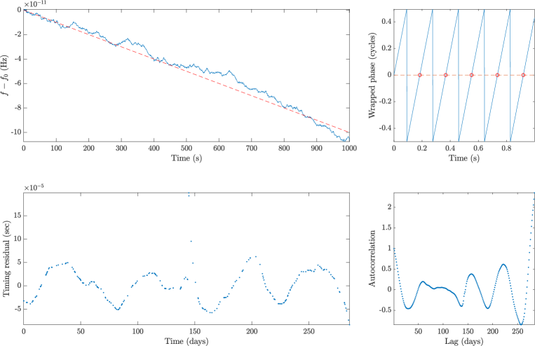
Figure 11: Sample segment of synthetic data comprising 250 TOAs over $286\,{\rm d}$ generated by solving (E1)–(E3) with a relatively large glitch injected at $t=144.67\,{\rm d}$. (Top left panel.) Stochastic frequency evolution $f(t)$ (blue solid curve) and deterministic component $f(0)+\dot{f}(0)t$ (red dashed curve) within the subinterval $0\leq t/(1\,{\rm s})\leq 10^{3}$. (Top right panel.) Wrapped phase versus time (blue solid curve) and TOA locations (red circles) within the window $0\leq t/(1\,{\rm s})\leq 1$. (Bottom left panel.) TOA residuals produced by a tempo2 fit to the data in the top left panel for $0\leq t/(1\,{\rm d})\leq 286$, which returns the best-fit parameters $(f_{\rm LS},\dot{f}_{\rm LS})=[f(0),\dot{f}(0)]+(-3.0\times 10^{-10}\,{\rm Hz},-5.9\times 10^{-18}\,{\rm Hz\,s^{-1}})$, $\Delta f_{\rm p}=5.2\times 10^{-8}\,{\rm Hz}$, $\Delta\dot{f}_{\rm p}=5.0\times 10^{-14}\,{\rm Hz\,s^{-1}}$, and glitch epoch $144.9\,{\rm d}$. (Bottom right panel.) Autocorrelation function of the phase residuals produced by the tempo2 fit in the bottom left panel. Injection parameters in (E1)–(E3): $f(0)=5.435\,{\rm Hz}$, $\dot{f}(0)=-1\times 10^{-13}\,{\rm Hz\,s^{-1}}$, $\sigma_{\rm TN}=5\times 10^{-13}\,{\rm Hz\,s^{-1/2}}$, $\Delta f_{\rm p}=5\times 10^{-8}\,{\rm Hz}$, $\Delta\dot{f}_{\rm p}=5\times 10^{-14}\,{\rm Hz\,s^{-1}}$, $\Delta f_{1}=5\times 10^{-8}\,{\rm Hz}$, $\tau=5\,{\rm d}$.

Equations (E1) and (E2) can be extended in several ways. As the system is linear and obeys the principle of superposition, it is easy to add more exponential recoveries with amplitudes $\Delta f_{k}$ and time-scales $\tau_{k}$ ($k>1$) by lifting the order of the system of differential equations and adding forcing terms proportional to $H(t-T)$ and $\delta(t-T)$ as in (E1) and (E2). One can also include a secular second derivative of the form $\langle\ddot{f}\rangle\propto f^{n}$.

The reader may notice a similarity between (E1) and (E2) and the two-component model of a neutron star interior (Baym et al., 1969), where $f$ and $f_{s}$ correspond to the spin frequencies of the rigid crust and neutron condensate respectively. The analogy may prove useful in future work, when interpreting physically the results of HMM-based glitch searches, but it is not pertinent to this paper. Here we merely exploit the mathematical correspondence, which renders (E1) and (E2) with $\zeta(t)=0$ equivalent to (19), in order to generate synthetic data. We emphasize that the dynamical model for generating synthetic data differs deliberately from the dynamical model governing the hidden state evolution in the HMM. For example, white noise fluctuations enter through the torque in (E1) [i.e. $\zeta(t)$] and through the torque derivative in (9) [i.e. $\xi(t)$]. This reflects the situation in practice astrophysically, where the dynamical model for timing noise is unknown. It also confirms the robustness of the HMM in light of the encouraging results in §6. Likewise, the permanent jumps $\Delta f_{\rm p}$ and $\Delta\dot{f}_{\rm p}$ in the HMM transition probability (10)–(12) do not match exactly the eponyomous variables in the synthetic data generation model (E1) and (E2), although they are related.

Appendix F Representative worked example: synthetic data

In this section, we illustrate how to apply the HMM in §3 and the model selection procedure in §4 to a sample of synthetic data generated according to the recipe in §5 and the parameters in the penultimate (typical) column in Table 1. The results are plotted in Figures 12 and 13. The worked example breaks out the steps in the analysis and introduces several useful diagnostics. It is a training run for the systematic performance tests in §6.

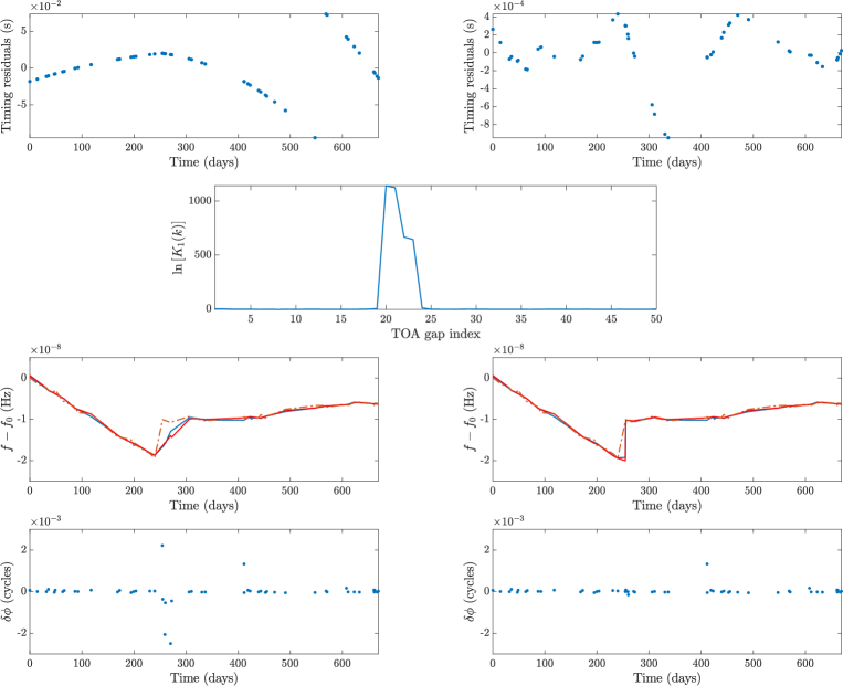
Figure 12: Worked example involving a segment of synthetic data generated by solving (E1)–(E3) with the parameters in the penultimate (typical) column in Table 1. (First row.) Phase residuals $\delta\phi(t_{n})$ versus TOA $t_{n}$ computed with tempo2 for no-glitch (left panel) and one-glitch (right panel) models with the parameters quoted in Appendix F. (Second row.) Logarithm of the Bayes factor, $K_{1}(k)=\Pr[O_{1:N_{T}}|M_{1}(k)]/\Pr(O_{1:N_{T}}|M_{0})$, versus TOA index, $k$, computed with the HMM using $\sigma=1\times 10^{-18}\,{\rm Hz\,s^{-3/2}}$. The glitch is injected at $k=19$ (epoch $T=253.371\,{\rm d}$) and recovered at $k=20$. (Third row.) Recovered frequency $f(t_{n})$ versus TOA $t_{n}$ for no-glitch (left panel) and one-glitch (right panel) models $M_{0}$ and $M_{1}(k=20)$, showing the injected signal (dash-dotted curve), HMM forward-backward sequence (blue curve), and HMM Viterbi sequence (red curve). (Fourth row.) Unsummed per-gap phase residuals $\delta\phi(t_{n})$ versus TOA $t_{n}$ for the HMM forward-backward sequences in the third row. The DOI and grid spacing are given by $-5.9\times 10^{-8}\leq(f-5.435\,{\rm Hz})/(1\,{\rm Hz})\leq 1\times 10^{-8}$, $-1\times 10^{-15}\leq\dot{f}/(1\,{\rm Hz\,s^{-1}})\leq 2\times 10^{-15}$, $\eta_{f}=6.79\times 10^{-11}\,{\rm Hz}$ ($10^{3}$ bins), and $\eta_{\dot{f}}=3\times 10^{-16}\,{\rm Hz\,s^{-1}}$ (11 bins).

The top two panels of Figure 12 present the raw data before any analysis with the HMM. The top left panel graphs the phase residuals $\delta\phi(t_{n})$ as a function of time after subtracting a no-glitch spin-down model with $f_{\rm LS}-5.435\,{\rm Hz}=1.48\times 10^{-8}\,{\rm Hz}$ and $\dot{f}_{\rm LS}=-1.41\times 10^{-15}\,{\rm Hz\,s^{-1}}$, inferred by fitting the full data set with tempo2. The residuals diverge for $t>T=253.371\,{\rm d}$ quadratically (and the phase wraps at $t\approx 550\,{\rm d}$), as expected for a glitch with $\Delta f_{\rm p}>0$ and $\Delta\dot{f}_{\rm p}>0$. Phase residuals are also plotted in the top right panel after subtracting a one-glitch model with $f_{\rm LS}-5.435\,{\rm Hz}=-1.2\times 10^{-10}\,{\rm Hz}$, $\dot{f}_{\rm LS}=-9.164\times 10^{-16}\,{\rm Hz\,s^{-1}}$, $T=254.37\,{\rm d}$, $\Delta f_{\rm p}=8.535\times 10^{-9}\,{\rm Hz}$, and $\Delta\dot{f}_{\rm p}=1.09\times 10^{-15}\,{\rm Hz\,s^{-1}}$, again fitted with tempo2. The residuals in the top right panel do not diverge and have root-mean-square amplitude $\sim 10^{-3}\,{\rm rad}$, consistent with $\sigma_{\rm TN}=1\times 10^{-12}\,{\rm Hz\,s^{-1/2}}$ integrated over $\sim 10^{2}\,{\rm d}$ ($\sigma_{\rm TN}$ dominates $\sigma_{\rm TOA}$ in this example). The fitted parameters are close to the injected parameters quoted in the penultimate column in Table 1. Returning to the no-glitch fit, we convert $\delta\phi(t_{n})$ into the DOI and grid spacing specified in the figure caption following the recipe in Appendix C.

Model selection is now performed. The second row of Figure 12 displays the Bayes factor, $K_{1}(k)=\Pr[O_{1:N_{T}}|M_{1}(k)]/\Pr(O_{1:N_{T}}|M_{0})$, as a function of the TOA index, $k$. The Bayes factor peaks at $\ln K_{1}(k_{1}^{\ast}=20)\sim 10^{3}$, well above the threshold $K_{1}(k)>10^{1/2}$. In other words, a model featuring a glitch near the injected location ($k=19$) is preferred categorically over the no-glitch model. The $\ln K_{1}(k)$ plateau near $k=k_{1}^{\ast}$ is typical of the HMM output for relatively large glitches, but the peak stands clearly above neighboring points, before the logarithm is taken. The single-TOA mismatch between the injected and recovered epochs is also typical. The HMM cannot say anything about the phase evolution between TOAs, so a single-TOA mismatch is always possible, even when a glitch is injected exactly at a TOA. Two-glitch models $M_{2}(k,l)$ are not considered here, as only one glitch is injected.

Finally, an ephemeris is constructed for the preferred model. The bottom four panels display $f(t_{n})$ (third row) and $\delta\phi(t_{n})$ (fourth row) as functions of $t_{n}$ for the point-wise optimal hidden sequence $\hat{q}(t_{n})$ found by the HMM forward-backward algorithm (blue curve) in Appendix A. For comparison, the sequence-wise optimal sequence $Q^{\ast}_{1:N_{T}}$ found by the Viterbi algorithm is also graphed (without residuals) as a red curve in the third row. Both HMM sequences lie close to each other and to the true, injected sequence, plotted as a dash-dotted curve. The forward-backward sequence $\hat{q}(t_{n})$ yields a root-mean-square error of $\approx 1\times 10^{-3}\,{\rm rad}$ for the one-glitch model $M_{1}(k_{1}^{\ast})$ (right column), which corresponds to $\approx 0.1\max_{n}\delta\phi(t_{n})$ for the no-glitch model $M_{0}$ (left column). The $M_{0}$ residuals are highest at $t\approx T$, as expected.

The posterior PDF of the hidden state likelihood in the neighborhood of the optimal sequence is a useful diagnostic. It indicates how far the optimal sequence stands out above its nearest competitors. It also provides a way of estimating point-by-point confidence intervals for the optimal ephemeris in practical astrophysical applications, where the underlying, true ephemeris is unknown. The top two panels in Figure 13 display heat map contours of the posterior PDF computed by the forward-backward algorithm, $\gamma_{q_{i}}(t_{n})$ in (A13), marginalized over $\dot{f}$ (first row) and $f$ (second row). The point-wise (forward-backward; blue curve) and sequence-wise (Viterbi; red curve) optimal state sequences run through the middle of the high-probability (yellow) regions. The bottom four panels display cross-sections of $\gamma_{q_{i}}(t_{n})$ immediately before (third row) and after (fourth row) the recovered glitch. The optimal state stands out clearly and is localized precisely. The FWHM of the PDF marginalized over $\dot{f}$ satisfies $\approx 1.4\times 10^{-10}\,{\rm Hz}$ and $\approx 4.8\times 10^{-10}\,{\rm Hz}$ before and after the glitch respectively, while the FWHM of the PDF marginalized over $f$ satisfies $\approx 3\times 10^{-16}\,{\rm Hz\,s^{-1}}$ and $\approx 6\times 10^{-16}\,{\rm Hz\,s^{-1}}$ before and after the glitch respectively. We can compute the jumps in $f$ and $\dot{f}$ during the glitch by comparing the peaks in the third and fourth rows. The displacements are clearly visible, once enough time elapses; we find $\hat{f}(t_{21})-\hat{f}(t_{19})=8.5\times 10^{-9}\,{\rm Hz}$ and $\hat{\dot{f}}(t_{21})-\hat{\dot{f}}(t_{19})=3\times 10^{-16}\,{\rm Hz\,s^{-1}}$, cf. the injected values $\Delta f_{\rm p}=1\times 10^{-8}\,{\rm Hz}$ and $\Delta\dot{f}_{\rm p}=1\times 10^{-15}\,{\rm Hz\,s^{-1}}$.

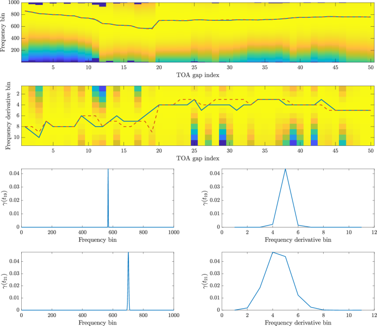
Figure 13: Evolution of the posterior PDF $\gamma_{q_{i}}(t_{n})$ defined by (A13) in the vicinity of the optimal values $\hat{f}(t_{n})$ and $\hat{\dot{f}}(t_{n})$. (First row.) Contours of $\gamma_{q_{i}}(t_{n})$ marginalized over $\dot{f}$ (arbitrary color scale; yellow high, blue low) versus TOA index $n$, with the point-wise optimal (forward-backward; blue curve) and sequence-wise optimal (Viterbi; red curve) state sequences overplotted. (Second row.) Contours of $\gamma_{q_{i}}(t_{n})$ marginalized over $f$ versus TOA index $n$. (Third row.) Cross-section of $\gamma_{q_{i}}(t_{n})$ marginalized over $\dot{f}$ (left column) and $f$ (right column) at $n=19$, i.e. at the TOA preceding the recovered glitch. The horizontal axes display numbers of bins. (Fourth row.) Cross-section of $\gamma_{q_{i}}(t_{n})$ marginalized over $\dot{f}$ (left column) and $f$ (right column) at $n=21$, i.e. at the TOA following the recovered glitch. Parameters: see Figure 12.

Appendix G Schedule of observations: impact on performance

When optimizing an observational campaign aimed at detecting glitches, it is important to plan how the spacing of observation sessions and the number of TOAs affect $P_{\rm fa}$ and $P_{\rm d}$. A typical observation session may last a few minutes, with $\sim 10^{4}$ pulses averaged to produce each TOA. Sessions are often separated by days to weeks, although of course there are exceptions; for instance, PSR J0835$-$4510 is monitored continuously for extended intervals (Palfreyman et al., 2016, 2018).

Figure 14 partially quantifies the above considerations. The left panel graphs $P_{\rm fa}$ and $P_{\rm d}$ as functions of the total number of observation sessions, after adjusting the Bayes factor threshold to achieve $P_{\rm fa}=10^{-2}$ on average across the plotted range. A detection is highly probable in most realistic scenarios; we obtain $P_{\rm d}\geq 0.9$ for $\gtrsim 35$ sessions. The right panel graphs $P_{\rm fa}$ and $P_{\rm d}$ as functions of the mean interval between sessions averaged over the entire observation ($\sim 1\,{\rm yr}$), after adjusting the Bayes factor threshold as in the left panel. We obtain $P_{\rm d}\geq 0.9$ for intervals between $\sim 10^{4}\,{\rm s}$ and $\sim 10^{6}\,{\rm s}$, which are readily achievable with dedicated or multibeam telescopes. For shorter intervals, the phase error due to $\sigma_{\rm TOA}$, which is independent of $\langle x_{n}\rangle$, impairs the HMM’s performance. For longer intervals, the phase error due to binning (see Appendix C) dominates, because it scales $\propto\langle x_{n}\rangle$. The results in Figure 14 are generated for one TOA per observation session. Tests show that $P_{\rm fa}$ is roughly constant given between one and five TOAs per session for the parameters in Figure 14. A thorough study of multiple TOAs per observation session, including the related and important matter of pulse jitter (Helfand et al., 1975), is postponed to future work.

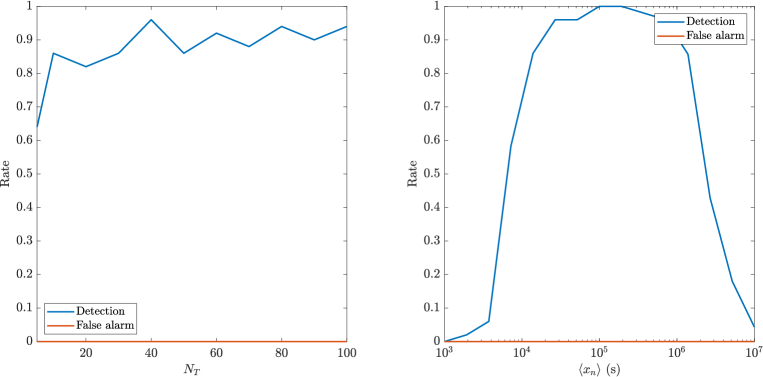
Figure 14: Detection probability (blue curve) and false alarm probability (red curve) versus the total number of observing sessions (left panel) and the mean TOA interval averaged over the entire observation (right panel). Parameters: as in Figure 3.

We formulate a useful rule of thumb to predict how one should space observations to resolve glitches of a certain size. During a gap of duration $x_{n}$, phase deviations $\Delta f_{\rm p}x_{n}$ and $\Delta\dot{f}_{\rm p}x_{n}^{2}/2$ develop for frequency and frequency derivative jumps respectively. Writing their ratio as $\approx(\Delta f_{\rm p}/f_{\rm LS})(\Delta\dot{f}_{\rm p}/\dot{f}_{\rm LS})^{-1}(x_{n}\dot{f}_{\rm LS}/f_{\rm LS})^{-1}$, we see that the two contributions are comparable typically, e.g. for $\Delta f_{\rm p}/f_{\rm LS}\sim 10^{-7}$, $\Delta\dot{f}_{\rm p}/\dot{f}_{\rm LS}\sim 10^{-2}$, and $x_{n}\dot{f}_{\rm LS}/f_{\rm LS}\sim 10^{-5}$. When the glitch-related phase deviations exceed those produced by TOA measurement errors ($\sigma_{\rm TOA}f_{\rm LS}$) and astrophysical timing noise ($\sigma_{\rm TN}x_{n}^{3/2}$), the glitch is discerned above the noise. This occurs for $\Delta f_{\rm p}\geq\sigma_{\rm TOA}f_{\rm LS}\langle x_{n}\rangle^{-1}$ and $\Delta f_{\rm p}\geq\sigma_{\rm TN}\langle x_{n}\rangle^{1/2}$ for $\Delta\dot{f}_{\rm p}=0$, or $\Delta\dot{f}_{\rm p}\geq 2\sigma_{\rm TOA}f_{\rm LS}\langle x_{n}\rangle^{-2}$ and $\Delta\dot{f}_{\rm p}\geq 2\sigma_{\rm TN}\langle x_{n}\rangle^{-1/2}$ for $\Delta f_{\rm p}=0$. Both special cases agree with the general expression for $\Delta f_{\rm p}\neq 0$ and $\Delta\dot{f}_{\rm p}\neq 0$ presented by Suvorova et al. (2018).

Another way to gauge the impact of the observational schedule on the HMM is to note that, when false alarms occur, they correlate with large TOA gaps. Figure 15 displays, in orange, a histogram of $x_{n}$ values adjacent to false alarms, along with a blue histogram of all the simulated $x_{n}$ values, whether they are adjacent to a false alarm or not. The simulations are in the regime, where $\ddot{f}$ can be neglected (see §3.2). As expected, there is a clear trend: false alarms occur more frequently near larger gaps, because the number of peaks in $L_{x_{n}q(t_{n})}$ within the DOI increases with $x_{n}$, even though the peaks sharpen (see §3.3). The correlation strengthens, as $\kappa$ and hence the number of false alarms increase. The opposite trend applies to false dismissals: the HMM is more prone to reject a true glitch, when $x_{n}$ is relatively short, because the phase deviation across the gap is relatively small.

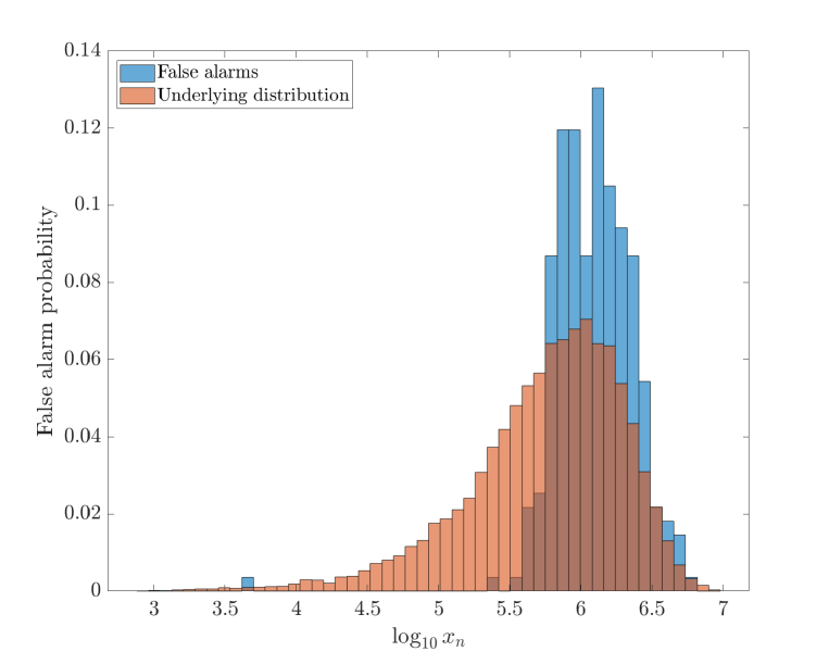
Figure 15: PDF of the logarithm of the TOA gap, $\log x_{n}$, for the subset of gaps adjacent to a false alarm (blue histogram) and for all simulated gaps (orange histogram; Poisson distribution by construction). Number of realizations: $5\times 10^{2}$. Other parameters: see penultimate (typical) column in Table 1.

Appendix H Is there a second glitch in PSR J0835$-$4510 between MJD 57427 and MJD 57810?

In this appendix, we apply the greedy hierarchical algorithm introduced in §4.2 (Suvorova et al., 2018) to test for the existence of a second glitch in PSR J0835$-$4510 in the interval from MJD 57427 to MJD 57810. Specifically, we assume that the glitch found at MJD 57734.54 is real and construct the model $M_{2}(173,k)$, which features a glitch at TOA interval $x_{173}$ and a second glitch at $x_{k}$.

Figure 16 presents the analysis of $M_{2}(173,k)$. The top panel displays the Bayes factor, $K_{2}(k)=\Pr[O_{1:N_{T}}|M_{2}(173,k)]/\Pr[O_{1:N_{T}}|M_{1}(173)]$, as a function of $k$. A peak is observed at $k=174$, with $\ln K_{2}(174)\approx 8$. Formally this counts as a detection by the criterion in §4.1. (The detection threshold in §4.1 is roughly consistent with $P_{\rm fa}\approx 1\times 10^{-2}$ and $P_{\rm d}\approx 0.9$ throughout this paper.) However, it occurs at the TOA immediately following the first glitch and is likely to be associated with it, because the introductory version of the HMM in this paper treats a glitch as an instantaneous step with no quasiexponential recovery, whereas in reality a recovery with $\tau=0.96(17)\,{\rm d}$ is measured independently in the 2016 December 12 event (Palfreyman, 2016; Sarkissian et al., 2017b). The second-highest peak in the top panel of Figure 16, which occurs at $k=123$ with $\ln K_{2}(123)\approx 1$, does not count as a detection by the criterion in §4.1.

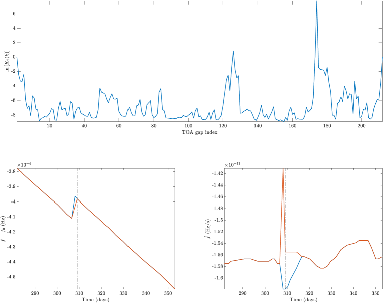
Figure 16: Search for a second glitch in PSR J0835$-$4510 between MJD 57427 and MJD 57810. (Top row.) Bayes factor $K_{2}(k)$ versus TOA index $k$. (Bottom row.) Point-wise optimal state sequence $\hat{f}(t_{n})$ (left panel) and $\hat{\dot{f}}(t_{n})$ (right panel) versus $t_{n}$ for the one-glitch model $M_{1}(173)$ (blue curves) and two-glitch model $M_{2}(173,174)$ (red curves). Parameters: see Figure 7.

The bottom left and right panels in Figure 16 display the point-wise optimal state sequences $\hat{f}(t_{n})$ and $\hat{\dot{f}}(t_{n})$ respectively, calculated by the forward-backward algorithm. The plots zoom into the neighborhood of the second “glitch” at $t_{174}$ (dashed vertical line) and compare the one-glitch model $M_{1}(173)$ (blue curve) with the two-glitch model $M_{2}(173,174)$ (red curve). Both models handle the complicated, composite dynamics of the spin up and quasiexponential recovery with equal dexterity but in slightly different ways, e.g. $\hat{\dot{f}}$ increases for $t>T$ in $M_{2}(173,174)$, decreases in $M_{1}(173)$, and asymptotes to its long-term, post-glitch value over $\sim 5\,{\rm d}$ in both cases.

We note in closing that the three-glitch Bayes factor $K_{3}(k)$ does not exceed $10^{1/2}$ for any $k$, i.e. there is no evidence in the above data for a third glitch.

References

- Abbott et al. (2019) Abbott B. P., Abbott R., Abbott T. D., Abraham S., Acernese F., Ackley K., Adams C., Adhikari R. X., Adya V. B., Affeldt C., et al. 2019, Phys. Rev. D, 100, 122002
- Abbott et al. (2017) Abbott B. P., Abbott R., Abbott T. D., Acernese F., Ackley K., Adams C., Adams T., Addesso P., Adhikari R. X., Adya V. B., et al. 2017, Phys. Rev. D, 95, 122003
- Anderson & Itoh (1975) Anderson P. W., Itoh N., 1975, Nature, 256, 25
- Archibald et al. (2016) Archibald R. F., Gotthelf E. V., Ferdman R. D., Kaspi V. M., Guillot S., Harrison F. A., Keane E. F., Pivovaroff M. J., Stern D., Tendulkar S. P., Tomsick J. A., 2016, ApJ, 819, L16
- Arzoumanian et al. (2016) Arzoumanian Z., Brazier A., Burke-Spolaor S., Chamberlin S. J., Chatterjee S., Christy B., Cordes J. M., Cornish N. J., Crowter K., Demorest P. B., et al. 2016, ApJ, 821, 13
- Arzoumanian et al. (1994) Arzoumanian Z., Nice D. J., Taylor J. H., Thorsett S. E., 1994, ApJ, 422, 671
- Ashton et al. (2019) Ashton G., Lasky P. D., Graber V., Palfreyman J., 2019, Nature Astronomy, 3, 1143
- Ashton et al. (2017) Ashton G., Prix R., Jones D. I., 2017, Phys. Rev. D, 96, 063004
- Bayley et al. (2019) Bayley J., Messenger C., Woan G., 2019, Phys. Rev. D, 100, 023006
- Baym et al. (1969) Baym G., Pethick C., Pines D., Ruderman M., 1969, Nature, 224, 872
- Calafiore & El Ghaoui (2014) Calafiore G. C., El Ghaoui L., 2014, Optimization Models. Cambridge: Cambridge University Press
- Carlin & Melatos (2019) Carlin J. B., Melatos A., 2019, MNRAS, 483, 4742
- Carlin et al. (2019) Carlin J. B., Melatos A., Vukcevic D., 2019, MNRAS, 482, 3736
- Chugunov & Horowitz (2010) Chugunov A. I., Horowitz C. J., 2010, MNRAS, 407, L54
- Coles et al. (2011) Coles W., Hobbs G., Champion D. J., Manchester R. N., Verbiest J. P. W., 2011, MNRAS, 418, 561
- Cordes (1980) Cordes J. M., 1980, ApJ, 237, 216
- Cordes & Downs (1985) Cordes J. M., Downs G. S., 1985, ApJS, 59, 343
- Cordes & Helfand (1980) Cordes J. M., Helfand D. J., 1980, ApJ, 239, 640
- D’Alessandro et al. (1995) D’Alessandro F., McCulloch P. M., Hamilton P. A., Deshpande A. A., 1995, MNRAS, 277, 1033
- Dunn et al. (2020) Dunn L., Clearwater P., Melatos A., Wette K., 2020, Classical and Quantum Gravity, p. submitted
- Edwards et al. (2006) Edwards R. T., Hobbs G. B., Manchester R. N., 2006, MNRAS, 372, 1549
- Espinoza et al. (2014) Espinoza C. M., Antonopoulou D., Stappers B. W., Watts A., Lyne A. G., 2014, MNRAS, 440, 2755
- Espinoza et al. (2011) Espinoza C. M., Lyne A. G., Stappers B. W., Kramer M., 2011, MNRAS, 414, 1679
- Faucher-Giguère & Kaspi (2006) Faucher-Giguère C.-A., Kaspi V. M., 2006, ApJ, 643, 332
- Fuentes et al. (2019) Fuentes J. R., Espinoza C. M., Reisenegger A., 2019, A&A, 630, A115
- Fulgenzi et al. (2017) Fulgenzi W., Melatos A., Hughes B. D., 2017, MNRAS, 470, 4307
- Gardiner (1994) Gardiner C. W., 1994, Handbook of stochastic methods for physics, chemistry and the natural sciences
- Glampedakis & Andersson (2009) Glampedakis K., Andersson N., 2009, Phys. Rev. Lett., 102, 141101
- Goncharov et al. (2019) Goncharov B., Zhu X.-J., Thrane E., 2019, arXiv e-prints, p. arXiv:1910.05961
- Haskell & Melatos (2015) Haskell B., Melatos A., 2015, International Journal of Modern Physics D, 24, 1530008
- Helfand et al. (1975) Helfand D. J., Manchester R. N., Taylor J. H., 1975, ApJ, 198, 661
- Hobbs & Dai (2017) Hobbs G., Dai S., 2017, ArXiv e-prints
- Hobbs et al. (2006) Hobbs G., Edwards R., Manchester R., 2006, Chinese Journal of Astronomy and Astrophysics Supplement, 6, 189
- Hobbs et al. (2009) Hobbs G., Hollow R., Champion D., Khoo J., et al. 2009, PASA, 26, 468
- Hobbs et al. (2004) Hobbs G., Lyne A. G., Kramer M., Martin C. E., Jordan C., 2004, MNRAS, 353, 1311
- Howitt et al. (2018) Howitt G., Melatos A., Delaigle A., 2018, ApJ, 867, 60
- Jankowski et al. (2019) Jankowski F., Bailes M., van Straten W., Keane E. F., et al. 2019, MNRAS, 484, 3691
- Janssen & Stappers (2006) Janssen G. H., Stappers B. W., 2006, A&A, 457, 611
- Jeffreys (1998) Jeffreys H., 1998, The Theory of Probability. Oxford: Oxford University Press (3rd ed.)
- Johnston & Galloway (1999) Johnston S., Galloway D., 1999, MNRAS, 306, L50
- Jones (1990) Jones P. B., 1990, MNRAS, 246, 364
- Lattimer & Prakash (2007) Lattimer J. M., Prakash M., 2007, Phys. Rep., 442, 109
- Leaci & Prix (2015) Leaci P., Prix R., 2015, Phys. Rev. D, 91, 102003
- Lentati et al. (2015) Lentati L., Alexander P., Hobson M. P., 2015, MNRAS, 447, 2159
- Lentati et al. (2014) Lentati L., Alexander P., Hobson M. P., Feroz F., van Haasteren R., Lee K. J., Shannon R. M., 2014, MNRAS, 437, 3004
- Lentati et al. (2018) Lentati L., Champion D. J., Kramer M., Barr E., Torne P., 2018, MNRAS, 473, 5026
- Lentati & et al. (2017) Lentati L., et al. 2017, MNRAS, 466, 3706
- Lentati et al. (2017) Lentati L., Kerr M., Dai S., Shannon R. M., Hobbs G., Osłowski S., 2017, MNRAS, 468, 1474
- Lentati & Shannon (2015) Lentati L., Shannon R. M., 2015, MNRAS, 454, 1058
- Lentati et al. (2015) Lentati L., Taylor S. R., Mingarelli C. M. F., Sesana A., Sanidas S. A., Vecchio A., Caballero R. N., Lee K. J., van Haasteren R., Babak S., et al. 2015, MNRAS, 453, 2576
- Lower et al. (2019) Lower M. E., Bailes M., Shannon R. M., Johnston S., Flynn C., Bateman T., Campbell-Wilson D., Day C. K., Deller A., Farah W., et al. 2019, Research Notes of the American Astronomical Society, 3, 192
- Lower et al. (2020) Lower M. E., Bailes M., Shannon R. M., Johnston S., Flynn C., Osłowski S., Gupta V., Farah W., Bateman T., Green A. J., Hunstead R., Jameson A., Jankowski F., Parthasarathy A., Price D. C., Sutherland A., Temby D., Krishnan V. V., 2020, MNRAS
- Lower et al. (2018) Lower M. E., Flynn C., Bailes M., Barr E. D., Bateman T., Bhandari S., Caleb M., Campbell-Wilson D., Day C., Deller A., et al. 2018, Research Notes of the American Astronomical Society, 2, 139
- Lyne & Graham-Smith (2012) Lyne A., Graham-Smith F., 2012, Pulsar Astronomy
- Lyne et al. (1996) Lyne A. G., Pritchard R. S., Graham-Smith F., Camilo F., 1996, Nature, 381, 497
- Lyne et al. (2000) Lyne A. G., Shemar S. L., Smith F. G., 2000, MNRAS, 315, 534
- Mardia & Jupp (2009) Mardia K. C., Jupp P. E., 2009, Directional Statistics
- McCulloch et al. (1987) McCulloch P. M., Klekociuk A. R., Hamilton P. A., Royle G. W. R., 1987, Australian Journal of Physics, 40, 725
- Melatos (1997) Melatos A., 1997, MNRAS, 288, 1049
- Melatos et al. (2018) Melatos A., Howitt G., Fulgenzi W., 2018, ApJ, 863, 196
- Melatos & Link (2014) Melatos A., Link B., 2014, MNRAS, 437, 21
- Melatos & Peralta (2010) Melatos A., Peralta C., 2010, ApJ, 709, 77
- Melatos et al. (2008) Melatos A., Peralta C., Wyithe J. S. B., 2008, ApJ, 672, 1103
- Melrose (2017) Melrose D. B., 2017, Reviews of Modern Plasma Physics, 1, 5
- Michel (1991) Michel F. C., 1991, Theory of neutron star magnetospheres. Chicago: University of Chicago Press
- Middleditch et al. (2006) Middleditch J., Marshall F. E., Wang Q. D., Gotthelf E. V., Zhang W., 2006, ApJ, 652, 1531
- Namkham et al. (2019) Namkham N., Jaroenjittichai P., Johnston S., 2019, MNRAS, 487, 5854
- Onuchukwu & Chukwude (2016) Onuchukwu C. C., Chukwude A. E., 2016, Ap&SS, 361, 300
- Palfreyman (2016) Palfreyman J., 2016, The Astronomer’s Telegram, 9847
- Palfreyman et al. (2018) Palfreyman J., Dickey J. M., Hotan A., Ellingsen S., van Straten W., 2018, Nature, 556, 219
- Palfreyman et al. (2016) Palfreyman J. L., Dickey J. M., Ellingsen S. P., Jones I. R., Hotan A. W., 2016, ApJ, 820, 64
- Parthasarathy et al. (2019) Parthasarathy A., Shannon R. M., Johnston S., Lentati L., Bailes M., Dai S., Kerr M., Manchester R. N., Osłowski S., Sobey C., van Straten W., Weltevrede P., 2019, MNRAS, 489, 3810
- Price et al. (2012) Price S., Link B., Shore S. N., Nice D. J., 2012, MNRAS, 426, 2507
- Quinn & Hannan (2001) Quinn B. G., Hannan E. J., 2001, The estimation and tracking of frequency. Cambridge: Cambridge University Press
- Rabiner (1989) Rabiner L. R., 1989, Proceedings of the IEEE, 77, 257
- Rickett (1990) Rickett B. J., 1990, ARA&A, 28, 561
- Sarkissian et al. (2017a) Sarkissian J., Reynolds J., Hobbs G., Harvey-Smith L., 2017a, CSIRO Data Collection; DOI 10.4225/08/59183e949e033
- Sarkissian et al. (2017b) Sarkissian J. M., Reynolds J. E., Hobbs G., Harvey-Smith L., 2017b, PASA, 34, e027
- Shannon et al. (2016) Shannon R. M., Lentati L. T., Kerr M., Johnston S., Hobbs G., Manchester R. N., 2016, MNRAS, 459, 3104
- Shannon et al. (2015) Shannon R. M., Ravi V., Lentati L. T., Lasky P. D., Hobbs G., Kerr M., Manchester R. N., Coles W. A., Levin Y., Bailes M., et al. 2015, Science, 349, 1522
- Stairs (2003) Stairs I. H., 2003, Living Reviews in Relativity, 6, 5
- Suvorova et al. (2017) Suvorova S., Clearwater P., Melatos A., Sun L., Moran W., Evans R. J., 2017, Phys. Rev. D, 96, 102006
- Suvorova et al. (2018) Suvorova S., Melatos A., Evans R. J., Moran W., 2018, IEEE Transactions on Signal Processing, p. submitted
- Suvorova et al. (2016) Suvorova S., Sun L., Melatos A., Moran W., Evans R. J., 2016, Phys. Rev. D, 93, 123009
- Taylor (1992) Taylor J. H., 1992, Philosophical Transactions of the Royal Society of London Series A, 341, 117
- van Eysden & Melatos (2010) van Eysden C. A., Melatos A., 2010, MNRAS, 409, 1253
- van Straten et al. (2012) van Straten W., Demorest P., Oslowski S., 2012, Astronomical Research and Technology, 9, 237
- Warszawski & Melatos (2011) Warszawski L., Melatos A., 2011, MNRAS, 415, 1611
- Watts et al. (2015) Watts A., Espinoza C. M., Xu R., Andersson N., Antoniadis J., Antonopoulou D., Buchner S., Datta S., Demorest P., Freire P., Hessels J., Margueron J., Oertel M., Patruno A., Possenti A., Ransom S., Stairs I., Stappers B., 2015, in Advancing Astrophysics with the Square Kilometre Array (AASKA14) Probing the neutron star interior and the Equation of State of cold dense matter with the SKA. p. 43
- Wette (2016) Wette K., 2016, Phys. Rev. D, 94, 122002
- Wong et al. (2001) Wong T., Backer D. C., Lyne A. G., 2001, ApJ, 548, 447
- Yakovlev et al. (1999) Yakovlev D. G., Levenfish K. P., Shibanov Y. A., 1999, Physics Uspekhi, 42, 737
- Yu & Liu (2017) Yu M., Liu Q.-J., 2017, MNRAS, 468, 3031
- Yu et al. (2013) Yu M., Manchester R. N., Hobbs G., Johnston S., Kaspi V. M., Keith M., Lyne A. G., Qiao G. J., Ravi V., Sarkissian J. M., Shannon R., Xu R. X., 2013, MNRAS, 429, 688