Exploring the evolution of stellar rotation using Galactic kinematics

Abstract

The rotational evolution of cool dwarfs is poorly constrained after $\sim$1-2 Gyr due to a lack of precise ages and rotation periods for old main-sequence stars. In this work we use velocity dispersion as an age proxy to reveal the temperature-dependent rotational evolution of low-mass Kepler dwarfs, and demonstrate that kinematic ages could be a useful tool for calibrating gyrochronology in the future. We find that a linear gyrochronology model, calibrated to fit the period–$T_{\mathrm{eff}}$ relationship of the Praesepe cluster, does not apply to stars older than around 1 Gyr. Although late-K dwarfs spin more slowly than early-K dwarfs when they are young, at old ages we find that late-K dwarfs rotate at the same rate or faster than early-K dwarfs of the same age. This result agrees qualitatively with semi-empirical models that vary the rate of surface-to-core angular momentum transport as a function of time and mass. It also aligns with recent observations of stars in the NGC 6811 cluster, which indicate that the surface rotation rates of K dwarfs go through an epoch of inhibited evolution. We find that the oldest Kepler stars with measured rotation periods are late-K and early-M dwarfs, indicating that these stars maintain spotted surfaces and stay magnetically active longer than more massive stars. Finally, based on their kinematics, we confirm that many rapidly rotating GKM dwarfs are likely to be synchronized binaries.

1 Introduction

1.1 Gyrochronology

Stars with significant convective envelopes ($\lesssim$ 1.3 M_⊙) have strong magnetic fields and slowly lose angular momentum via magnetic braking (e.g. Schatzman, 1962; Weber & Davis, 1967; Kraft, 1967; Skumanich, 1972; Kawaler, 1988; Pinsonneault et al., 1989). Although stars are born with random rotation periods, between 1 and 10 days, observations of young open clusters reveal that their rotation periods converge onto a unique sequence by $\sim$500-700 million years (e.g. Irwin & Bouvier, 2009; Gallet & Bouvier, 2013). After this time, the rotation period of a star is thought to be determined, to first order, by its color and age alone. This is the principle behind gyrochronology, the method of inferring a star’s age from its rotation period (e.g. Skumanich, 1972; Barnes, 2003, 2007; Mamajek & Hillenbrand, 2008; Barnes, 2010; Meibom et al., 2011, 2015). However, new photometric rotation periods made available by the Kepler (Borucki et al., 2010) and K2 (Howell et al., 2014) missions (e.g. McQuillan et al., 2014; García et al., 2014; Douglas et al., 2017; Rebull et al., 2017; Meibom et al., 2011, 2015; Curtis et al., 2019) confirm that rotational evolution is a highly complex process. For example, the early-to-mid M dwarfs in the $\sim$ 650 Myr Praesepe cluster spin more slowly than the G dwarfs; in theory because lower-mass stars have deeper convective zones which generate stronger magnetic fields and more efficient magnetic braking. However, in the NGC 6811 cluster which is around 1 Gyr (Janes & Hoq, 2011; Sandquist et al., 2016), late-K dwarfs rotate at the same rate as early-K dwarfs (Curtis et al., 2019). In addition, new rotation period measurements for low-mass stars in the 2.7-Gyr-old cluster Ruprecht 147 show that its slow-rotator sequence is flat compared to younger clusters like Praesepe (Curtis et al. 2020, submitted to AAS Journals), and departures from classical Skumanich-like spin-down were also noted in observations of the $\sim$1.3 Gyr NGC 752 open cluster (Agüeros et al., 2018). New semi-empirical models that vary the rate of angular momentum redistribution in the interiors of stars are able to reproduce the flattened period–color relation seen in these clusters (Spada & Lanzafame, 2019). These models suggest that mass and age-dependent angular momentum transport between the cores and envelopes of stars has a significant impact on their surface rotation rates.

Another example of unexpected rotational evolution is seen in old field stars which appear to rotate more rapidly than classical gyrochronology models predict (Angus et al., 2015; van Saders et al., 2016, 2018; Metcalfe & Egeland, 2019). A mass-dependent modification to the classical $P_{\mathrm{rot}}$ $\propto t^{\frac{1}{2}}$ spin-down law (Skumanich, 1972) is required to reproduce these observations. To fit magnetic braking models to these data, a cessation of magnetic braking is required after stars reach a Rossby number (Ro; the ratio of rotation period to convective turnover time) of around 2 (van Saders et al., 2016, 2018).

The rotational evolution of stars is clearly a complicated process and, to fully calibrate the gyrochronology relations we need a large sample of reliable ages for stars spanning a range of ages and masses. In this paper, we use the velocity dispersions of field stars to qualitatively explore the rotational evolution of GKM dwarfs, and show that kinematics could provide a gyrochronology calibration sample.

1.2 Using velocity dispersion as an age proxy

Stars are thought to be born in the thin disk of the Milky Way (MW), orbiting the Galaxy with a low out-of-plane, or vertical, velocity ($v_{\bf z}$), just like the star-forming molecular gas observed in the disk today (e.g. Stark & Brand, 1989; Stark & Lee, 2005; Aumer & Binney, 2009; Martig et al., 2014; Aumer et al., 2016). On average, the vertical velocities of older stars is observed to be larger (e.g. Nordström et al., 2004; Holmberg et al., 2007, 2009; Aumer & Binney, 2009; Casagrande et al., 2011). This is likely either a signature of dynamical heating, such as from interactions with giant molecular clouds, spiral arms and the galactic bar (see Sellwood, 2014, for a review of secular evolution in the MW), or an indication that stars formed dynamically “hotter” in the past (e.g., Bird et al., 2013). In either case, the vertical velocity distribution is observed to depend significantly on stellar age. While the velocity of any individual star only provides a weak age constraint (if any at all), because its velocity depends on its current position in its orbit, the velocity dispersion of a population of stars indicates whether that population is old or young relative to other populations. In this work, we compare the velocity dispersions of populations of field stars in the Galactic thin disk to ascertain which populations are older and which younger, and draw conclusions about the rotational evolution of stars based on their implied relative ages.

There is a long history of using kinematic ages to explore the evolution of cool dwarfs (e.g. Reid et al., 1995; Gizis et al., 2000; West et al., 2004, 2006; Schmidt et al., 2007; Faherty et al., 2009; Kiman et al., 2019). For example, West et al. (2004, 2006) used the vertical distances of stars from the Galactic mid-plane as an age proxy, and found that the fraction of magnetically active M dwarfs decreases over time. Faherty et al. (2009) used tangential velocities to infer the ages of M, L and T dwarfs, and showed that dwarfs with lower surface gravities tended to be kinematically younger, and Kiman et al. (2019) used velocity dispersion as an age proxy to explore the evolution of H$\alpha$ equivalent width (a magnetic activity indicator), in M dwarfs.

Although vertical velocity, $v_{\bf z}$, is a well-established age proxy, it can only be calculated with full 6-dimensional position and velocity information. In fact, with full 6D phase space and an assumed Galactic potential, it is possible to calculate the dynamically-invariant vertical action, which may be an even better age indicator (Beane et al., 2018; Ting & Rix, 2019). Unfortunately, most field stars with measured rotation periods do not have radial velocity (RV) measurements because they are relatively faint Kepler targets ($\sim$12th-16th magnitudes). For this reason, we used velocity in the direction of galactic latitude, $v_{\bf b}$, as a proxy for $v_{\bf z}$. The Kepler field is positioned at low galactic latitude (b=$\sim$5-20^∘), so $v_{\bf b}$ is a close (although imperfect, see appendix) approximation to $v_{\bf z}$. Because we use $v_{\bf b}$ rather than $v_{\bf z}$  we do not calculate absolute kinematic ages using a published age–velocity dispersion relation (AVR), calibrated with vertical velocity. In the future it may be possible to account for the differences between $v_{\bf b}$ and $v_{\bf z}$, or marginalize over missing RV measurements and the Kepler selection function, in order to infer the absolute ages of populations of stars. Regardless of direction however, velocity dispersion is expected to monotonically increase over time (e.g. Holmberg et al., 2009), and can therefore be used to rank populations of stars by age.

This paper is laid out as follows: in section 2 we describe our sample selection process and the methods used to calculate stellar velocities. In section 3 we use kinematics to investigate the relationship between stellar rotation period, age and color/$T_{\mathrm{eff}}$ and interpret the results. We also examine the rotation period gap and the kinematics of synchronized binaries. In the appendix, we establish that $v_{\bf b}$ velocity dispersion, $\sigma_{v{\bf b}}$, can be used as an age proxy by demonstrating that neither mass-dependent heating nor the Kepler/Gaia selection function is observed to strongly affect our sample. The data used in this project is described in table 2, at the end of this paper, and is available online.

2 Method

2.1 The data

We used the publicly available Kepler-Gaia DR2 crossmatched catalog to combine the McQuillan et al. (2014) catalog of stellar rotation periods, measured from Kepler light curves, with the Gaia DR2 catalog of parallaxes, proper motions and apparent magnitudes. Reddening and extinction from dust was calculated for each star using the Bayestar dust map implemented in the dustmaps Python package (Green, 2018), and astropy (Astropy Collaboration et al., 2013, 2018). For this work, we used the precise Gaia DR2 photometric color, $G_{\rm BP}-G_{\rm RP}$, to estimate $T_{\mathrm{eff}}$ for the Kepler rotators. The calibration of this relation is described in Curtis et al. (2020, in prep) and summarized in the Appendix of this paper.

Photometric binaries and subgiants were removed from the McQuillan et al. (2014) sample by applying cuts to the color-magnitude diagram (CMD), shown in figure 1. A 6th-order polynomial was fit to the main sequence and raised by 0.27 dex to approximate the division between single stars and photometric binaries (shown as the curved dashed line in figure 1). All stars above this line were removed from the sample. Potential subgiants were also removed by eliminating stars brighter than 4th absolute magnitude in Gaia G-band. This cut also removed a number of main sequence F stars from our sample, however these hot stars are not the focus of our gyrochronology study since their small convective zones inhibit the generation of a strong magnetic field. The removal of photometric binaries and evolved/hot stars reduced the total sample of around 34,000 stars by almost 10,000.

The rotation periods of the dwarf stars in the McQuillan et al. (2014) sample are shown on a Gaia color-magnitude diagram (CMD) in the top panel of figure 1. In the bottom panel, the stars are colored by their gyrochronal age, calculated using the Angus et al. (2019) gyrochronology relation. The stars with old gyrochronal ages, plotted in purple hues, predominantly lie along the upper edge of the MS, where stellar evolution models predict old stars to be, however the majority of these ‘old’ stars are bluer than $G_{BP}-G_{RP}$ $\sim$ 1.5 dex. The lack of gyrochronologically old M dwarfs suggests that either old M dwarfs are missing from the McQuillan et al. (2014) catalog, or the Angus et al. (2019) gyrochronology relation under-predicts the ages of low-mass stars. Given that lower-mass stars stay active for longer than higher-mass stars (e.g. West et al., 2008; Newton et al., 2017; Kiman et al., 2019), and are therefore more likely to have measurable rotation periods at old ages, the latter scenario seems likely. However, it is also possible that the rotation periods of the oldest early M dwarfs are so long that they are not measurable with Kepler data. Ground-based rotation period measurements of early M dwarfs (spectral types earlier than $\sim$ M2.5, $T_{\mathrm{eff}}$ $\gtrsim$ 3500 K) indicate there is a $\sim$ 80 day upper limit to their rotation periods (Newton et al., 2016, 2018), which is longer than the longest rotation periods measured for the early M dwarfs in the McQuillan et al. (2014) sample (around 50 days).

The apparent lack of old gyro-ages for M dwarfs in figure 1 may be caused by a combination of ages being underestimated by a poorly calibrated model, and rotation period detection bias. The Angus et al. (2019) gyrochronology relation is a simple polynomial model, fit to the period-color relation of Praesepe. Inaccuracies at low masses are a typical feature of empirically calibrated gyrochronology models since there are no (or at least very few) old M dwarfs with rotation periods and the models are poorly calibrated for these stars.

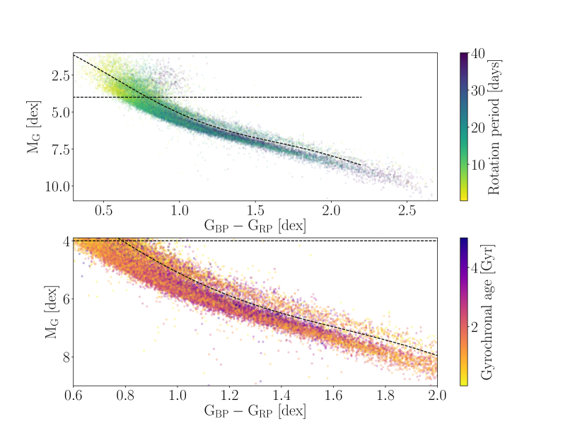
Figure 1: Top: de-reddened MS Kepler stars with McQuillan et al. (2014) rotation periods, plotted on a Gaia CMD. We removed photometric binaries and subgiants from the sample by excluding stars above the dashed lines. Bottom: a zoom-in of the top panel, with stars colored by their gyrochronal age (Angus et al., 2019), instead of their rotation period. A general age gradient is visible across the main sequence. Since the Angus et al. (2019) relation predicts that the oldest stars in the McQuillan et al. (2014) sample are late-G and early-K dwarfs, it is probably under-predicting the ages of late-K and early-M dwarfs.

The Pyia (Price-Whelan, 2018) and astropy (Astropy Collaboration et al., 2013, 2018) Python packages were used to calculate velocities for the McQuillan et al. (2014) sample. Pyia calculates velocity samples from the full Gaia uncertainty covariance matrix via Monte Carlo sampling, thereby accounting for the covariances between Gaia positions, parallaxes and proper motions. Stars with negative parallaxes or parallax signal-to-noise ratios less than 10 (around 3,000 stars), stars fainter than 16th magnitude in Gaia G-band (200 stars), stars with absolute $v_{\bf b}$ uncertainties greater than 1 kms^-1 (1000 stars), and stars with galactic latitudes greater than 15^∘ (5500 stars, justification provided in the appendix) were removed from the sample. Finally, we removed almost 2000 stars with rotation periods shorter than the main population of periods, since this area of the period-$T_{\mathrm{eff}}$ diagram is sparsely populated. We removed these rapid rotators by cutting out stars with gyrochronal ages less than 0.5 Gyr (based on the Angus et al., 2019, gyro-model), because a 0.5 Gyr gyrochrone traces the bottom edge of the main population of rotation periods. These rapid rotators are probably either very young stars, or synchronized binaries (see section 3.3). After these cuts, around 13,000 stars out of the original $\sim$34,000 were included in the sample.

3 Results and Discussion

3.1 The period-$T_{\mathrm{eff}}$ relations, revealed

To explore the relationship between rotation period, effective temperature ($T_{\mathrm{eff}}$) and velocity dispersion, we calculated $\sigma_{v{\bf b}}$ for populations of stars with similar rotation periods and temperatures, and presumed similar age. The top panel of figure 2 shows rotation period versus effective temperature for the McQuillan et al. (2014) sample, coloured by $\sigma_{v{\bf b}}$, where $\sigma_{v{\bf b}}$ was calculated for groups of stars over a grid in $\log_{10}$(period) and temperature. If we assume that mass dependent heating does not strongly affect this sample and $v_{\bf b}$ at low galactic latitudes is an unbiased tracer of $v_{\bf z}$, then $v_{\bf b}$ velocity dispersion can be interpreted as an age proxy, and stars plotted in a similar color in figure 2 are similar ages. In the appendix of this paper, we show that this assumption appears valid for stars with Galactic latitude $<$ 15^∘.

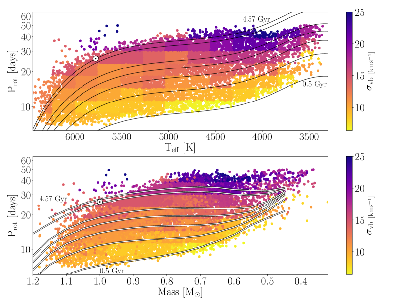
Figure 2: Top: Rotation period vs effective temperature for stars in the McQuillan et al. (2014) sample, colored by the velocity dispersions of stars calculated over a grid in $\log_{10}$(period) and $T_{\mathrm{eff}}$ (this grid causes the quantized appearance). Black lines show gyrochrones from a gyrochronology model that projects the rotation-color relation of Praesepe to longer rotation periods over time (Angus et al., 2019). These gyrochrones do not appear to reflect the evolution of field stars at long rotation periods/old ages because they do not trace lines of constant velocity dispersion. Gyrochrones are plotted at 0.5, 1, 1.5, 2, 2.5, 4 and 4.57 Gyr (Solar age) in both top and bottom panels. Bottom: Same as top panel with rotation period vs mass (from Berger et al., 2020). White lines show gyrochrones from a model that includes mass and age-dependent angular momentum transport between the core and envelope (Spada & Lanzafame, 2019). Qualitatively, these gyrochrones reflect the evolution of field stars at long rotation periods/old ages: they trace lines of constant velocity dispersion by reproducing periods of ‘stalled’ surface rotational evolution for K-dwarfs. The data used to create this figure is available in table 2.

Overall, figure 2 shows that velocity dispersion increases with rotation period across all temperatures, implying that rotation period increases with age, as expected. This result is insensitive to the choice of bin position and size. Black lines show gyrochrones from the Angus et al. (2019) gyrochronology model, which projects the rotation-color relation of Praesepe to longer rotation periods over time. These gyrochrones are plotted at 0.5, 1, 1.5, 2, 2.5, 4 and 4.57 (Solar age) Gyr. At the youngest ages, these gyrochrones describe the data well: the palest yellow (youngest) stars with the lowest velocity dispersions all fall close to the 0.5 Gyr gyrochrone. However, although the 0.5 Gyr and 1 Gyr gyrochrones also trace constant velocity dispersion/age among the field stars, by 1.5 Gyr the gyrochrones start to cross different velocity dispersion regimes. For example, the 1.5 Gyr gyrochrone lies on top of stars with velocity dispersions of around 10-11 kms^-1 at 5000-5500K and stars with $\sim$15 kms^-1 velocity dispersions at 4000-4500K. The gyrochrones older than 1.5 Gyr also cross a range of velocity dispersions. If these were true isochrones they would follow lines of constant velocity dispersion. At ages older than around 1 Gyr, it appears that gyrochrones should have a more flattened, or even inverted, shape in rotation period-$T_{\mathrm{eff}}$ space than these Praesepe-based models.

The bottom panel of figure 2 shows velocity dispersion as a function of rotation period and mass, (from Berger et al., 2020), with gyrochrones from the Spada & Lanzafame (2019) model shown in white. These gyrochrones are plotted for the same ages described above. Each point plotted in the top panel also appears in the bottom panel with the same color. Because velocity dispersion was calculated in bins of $T_{\mathrm{eff}}$, not mass, bin outlines are clearly visible in the top panel but appear smeared-out in the bottom panel. In the bottom panel of figure 2, the Spada & Lanzafame (2019) models do trace lines of constant velocity dispersion, and reproduce the trends in the data at all ages. These models qualitatively agree with the data and reproduce the apparent flattening and inversion in the rotation period-$T_{\mathrm{eff}}$/mass relations.

The results shown in figure 2 indicate that stars of spectral type ranging from late G to late K ($\sim$5500-3500 K) follow a braking law that changes over time. In particular, the relationship between rotation period and effective temperature appears to flatten out and eventually invert. These results provide further evidence for ‘stalled’ surface rotational evolution of K dwarfs, like that observed in open clusters (Curtis et al., 2019) and reproduced by models that vary angular momentum transport between stellar core and envelope with time and mass (Spada & Lanzafame, 2019).

The velocity dispersions of stars in the McQuillan et al. (2014) sample, shown in figure 2, provide the following picture of rotational evolution. At young ages (younger than around 1 Gyr but still old enough to be on the main sequence and have transitioned from the ‘C’ sequence to the ‘I’ sequence Barnes, 2003), stellar rotation period decreases with increasing mass. This is likely because lower-mass stars with deeper convection zones have stronger magnetic fields, larger Alfvén radii and therefore experience greater angular momentum loss rate (e.g. Schatzman, 1962; Kraft, 1967; Parker, 1970; Kawaler, 1988; Charbonneau, 2010; Matt et al., 2012, 2015). According to the Spada & Lanzafame (2019) model, the radiative cores and convective envelopes of stars are decoupled at these young ages, i.e. transportation of angular momentum from the surface to the core of the star is reduced, so the surface slows down due to wind-braking but the core keeps spinning rapidly. According to the data presented in figure 2, at intermediate ages, the rotation periods of K dwarfs appear constant with mass, and at late ages rotation period increases with increasing mass. The interpretation of this, according to the Spada & Lanzafame (2019) model, is that lower-mass stars are still braking more efficiently at these intermediate and old ages compared to higher-mass stars, but their cores are more tightly coupled to their envelopes, allowing angular momentum transport between the two layers. Angular momentum surfaces from the core and prevents the stellar envelopes from spinning-down rapidly, and this effect is strongest for late K-dwarfs with effective temperatures of $\sim$4000-4500K and masses $\sim$0.5-0.7 M_⊙.

A period of core-envelope decoupling in the evolution of cool dwarfs has been explored in theoretical models for decades (e.g. Endal & Sofia, 1981; MacGregor & Brenner, 1991; Denissenkov et al., 2010; Gallet & Bouvier, 2013). In such models, the angular momenta of the radiative core and convective envelope are permitted to evolve separately once a radiative core develops on the pre-main sequence. A decoupled core and envelope is required to reproduce observations of young clusters and star forming regions (e.g. Irwin et al., 2007; Bouvier, 2008; Denissenkov et al., 2010; Spada et al., 2011; Reiners & Mohanty, 2012) and has become an established element of theoretical gyrochronology models. During this phase, angular momentum transport between the radiative core and the convective envelope is reduced. Over time, models increase the efficiency of angular momentum transport between the core and envelope in order to reproduce the close-to solid body rotation observed for the Sun (e.g. Thompson et al., 1996). The core-envelope coupling timescale affects the predicted surface rotation periods of young and intermediate-age stars and is usually constrained using observations of open clusters. The Lanzafame & Spada (2015) gyrochronology model uses a mass-dependent core-envelope coupling timescale, and Spada & Lanzafame (2019) fit this model to open-cluster observations, including new rotation period measurements for K dwarfs in the NGC 6811 cluster (Curtis et al., 2019). A similar mass-dependent core-envelope coupling timescale was also found to explain the observed lithium depletion trends in open clusters by an independent study (Somers & Pinsonneault, 2016). Although variable angular momentum transport between the surfaces and cores of stars has been an essential ingredient of stellar evolution models for decades, the transport mechanism is still unknown. Among the proposed mechanisms are magneto-hydrodynamical waves resulting from various magnetic field geometries, and gravity waves (see, e.g. Charbonneau & MacGregor, 1993; Ruediger & Kitchatinov, 1996; Spruit, 2002; Talon & Charbonnel, 2003; Spada et al., 2010; Brun et al., 2011; Oglethorpe & Garaud, 2013).

In the top panel of figure 2, the Angus et al. (2019) gyrochronology model is plotted for comparison with the data. This model was chosen as an example but there are many other empirical gyrochronology models we could have used. All the available empirical gyrochronology models are similar in essence to the Angus et al. (2019) relation and, like that relation, none is able to reproduce the observed velocity dispersions, or capture the evolving shape of the period-$T_{\mathrm{eff}}$ relations.

The Angus et al. (2019) relation is a new fully-empirical gyrochronology relation, calibrated using recently measured rotation periods for members of the Praesepe cluster, which extend down to early M dwarfs (Rebull et al., 2017; Douglas et al., 2017). These are the oldest cluster M dwarfs with measured photometric rotation periods and the Angus et al. (2019) model therefore encapsulates the behavior of these cool stars at Praesepe age. Most semi-empirical spin-down models predict that, once the rotation periods of stars converge to a tight sequence, they approximately spin down with a common braking index (e.g., Fig. 5 in Gallet & Bouvier, 2015). So, if stellar rotation periods have fully converged by the age of Praesepe, as the observations suggest they have (Douglas et al., 2019), it is appropriate to project the Praesepe sequence forward in time with a single braking index that is common to all stars and constant in time. However, observations of low-mass stars in older clusters (e.g., NGC 6811, NGC 752, and Ruprecht 147 Curtis et al., 2019; Agüeros et al., 2018, Curtis et al. 2020, submitted) now demonstrate that the assumptions adopted in the semi-empirical models which support a common braking index must be invalid, or inaccurate in some quantitative way (for example, the core-envelope coupling timescale is inaccurately calibrated).

There are many other empirical gyrochronology models we could have chosen to compare with our data. For example, the Barnes (2003, 2007); Mamajek & Hillenbrand (2008); Meibom et al. (2011); Angus et al. (2015) relations all have a functional form that was first introduced by Barnes (2003): $\mathrm{P_{rot}}=t^{n}~{}a(B-V-c)^{b}$, where n, a, b and c are free parameters, and B and V are photometric magnitudes. These relations have been widely used in the literature, and are similar to the Angus et al. (2019) relation in that they consist of a color-dependent term multiplied by an age-dependent term, i.e. they are separable in color and age. None of these relations follow lines of constant velocity dispersion in figure 2 because they have a universal power-law index, $n$ ($\approx$ 0.5, Skumanich, 1972), which applies to stars of all masses and ages. They do not have the flexibility to capture the evolving period-color relationship seen in the data. The Barnes (2010) model has a different functional form: it uses Rossby number ($Ro=P_{\mathrm{rot}}/\tau$, where $\tau$ is the convective turnover time) to encode the mass-dependent evolution of rotation periods: $\frac{dP_{\mathrm{rot}}}{dt}\propto 1/Ro$. This simple relation neatly reproduces the rotation periods of stars in the slow-rotation sequences of young ($\sim$100-700 Gyr) clusters, however, like the other empirical gyrochronology models, it does not reproduce the observed trends seen in the velocity dispersion data here. The Barnes (2010) model has a similar period-$T_{\mathrm{eff}}$ relation to the Praesepe-based Angus et al. (2019) model, because the period-$T_{\mathrm{eff}}$ relation of Praesepe roughly follows a line of constant Rossby number. Consequently, like the Angus et al. (2019) model, the Barnes (2010) model in its current form does not have the flexibility to capture the mass and time-variable rotational evolution revealed by the data explored here.

It is not surprising that the Angus et al. (2019) model, or other gyrochronology models do not reproduce the data, since tensions with Skumanich-like spin-down have been revealed whenever new rotation periods of benchmark stars have become available (Angus et al., 2015; van Saders et al., 2016; Metcalfe & Egeland, 2019; Agüeros et al., 2018; Curtis et al., 2019). With the influx of new stellar rotation periods provided by Kepler/K2, TESS, and ground-based facilities, our understanding of spin-down is changing rapidly. New data are revealing flaws in not just the calibration of but also the functional forms of old models. We have shown that velocity dispersion data provides support for more sophisticated models that incorporate additional physical effects (e.g., core-envelope coupling Spada & Lanzafame, 2019) over the simple empirical models used today. Alternatively, more flexible empirical frameworks, like a Gaussian process model, could capture everything we now know about stellar spin-down.

3.2 The mass-dependence of magnetic activity lifetimes

The mass dependence of magnetic activity lifetimes has been demonstrated previously for M dwarfs (e.g. West et al., 2008; Reiners & Basri, 2008; West et al., 2009; Newton et al., 2017; Kiman et al., 2019) and, if the detectability of a rotation period is considered to be a magnetic activity proxy, then our results provide further evidence for a mass-dependent activity lifetime.

In order to measure a rotation period at all, there must be some magnetically active regions (either bright plages or dark spots), of a reasonable size on the surface of a star. In other words, some minimum magnetic activity level is presumably required to produce coherent light curve-variability, from which a rotation period can be confidently measured. The relatively sharp upper-edge of the rotation period distribution seen in figure 2 may therefore be caused by a finite active lifetime of stars, i.e. stars older than a critical age are no longer active enough to produce periodic, high-amplitude variability. In figure 2, the velocity dispersions of stars along the upper edge of the rotation period distribution increase with decreasing mass, indicating that magnetic activity lifetimes are mass-dependent. Figure 2 shows that the populations of stars with the largest velocity dispersions are cooler than 4500 K. This implies that most of the oldest stars with detectable rotation periods are cooler than 4500 K, i.e. these-low mass stars stay active longer than more massive stars.

To investigate this idea further, we compared the velocity dispersions of stars with measured rotation periods to the velocity dispersions of the entire Kepler sample. If stars with measured rotation periods are more magnetically active, and younger, than stars without rotation period measurements, they should also have smaller velocity dispersions. To test this theory, we calculated the velocity dispersions for all stars in the Kepler field (after removing visual binaries, subgiants, stars fainter than 16th magnitude, and high Galactic latitude stars, following the method described in section 2). We then compared these velocity dispersions, as a function of $T_{\mathrm{eff}}$, to the velocity dispersions of stars with measured rotation periods (i.e. stars that appear in table 1 of McQuillan et al., 2014). We show the ratio of total $\sigma_{v{\bf b}}$ to McQuillan-$\sigma_{v{\bf b}}$ as a function of $T_{\mathrm{eff}}$ in figure 3. A larger ratio means the rotating star sample is younger, on average, than the overall Kepler population, and a ratio of 1 means that the rotating stars have the same age distribution as the overall Kepler sample. Figure 3 shows that this ratio is largest for G stars and approaches unity for K and early M dwarfs. This indicates that the G stars with detectable rotation periods are, on average, younger than the total population of G stars in the Kepler field. On the other hand, the late K and early M dwarfs with detectable rotation periods have a similar age distribution to the overall Kepler population which suggests that most of the oldest K and M dwarfs are represented in the McQuillan et al. (2014) sample. This result bolsters the evidence that M dwarf rotation periods are measurable at older ages than G dwarf rotation periods and that G stars become magnetically inactive and have fewer active surface regions at a younger age than M dwarfs.

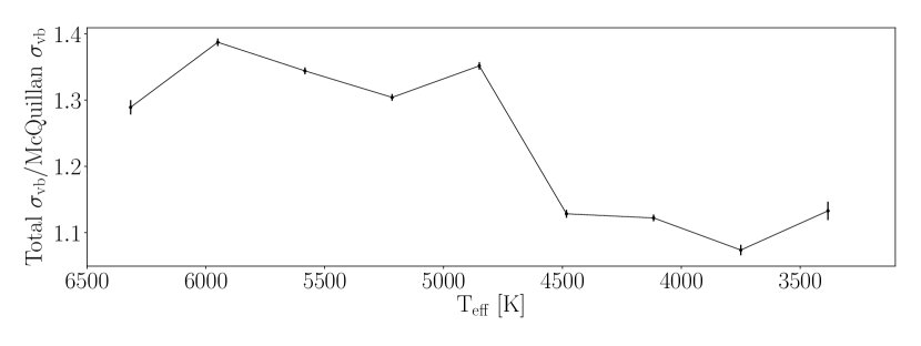
Figure 3: Velocity dispersions for the entire Kepler field divided by the velocity dispersions of stars with measured rotation periods in McQuillan et al. (2014), as a function of effective temperature. A larger ratio indicates that the overall Kepler field is older, on average, than stars in the McQuillan et al. (2014) catalog. As this ratio approaches unity the two populations have similar kinematic ages. The large ratio for the hottest stars indicates that G dwarfs become inactive at young ages. This ratio approaches unity at low temperatures, showing that K and early M dwarf rotation periods are measurable over a large range of ages.

3.3 Synchronized binaries and the Kepler period gap

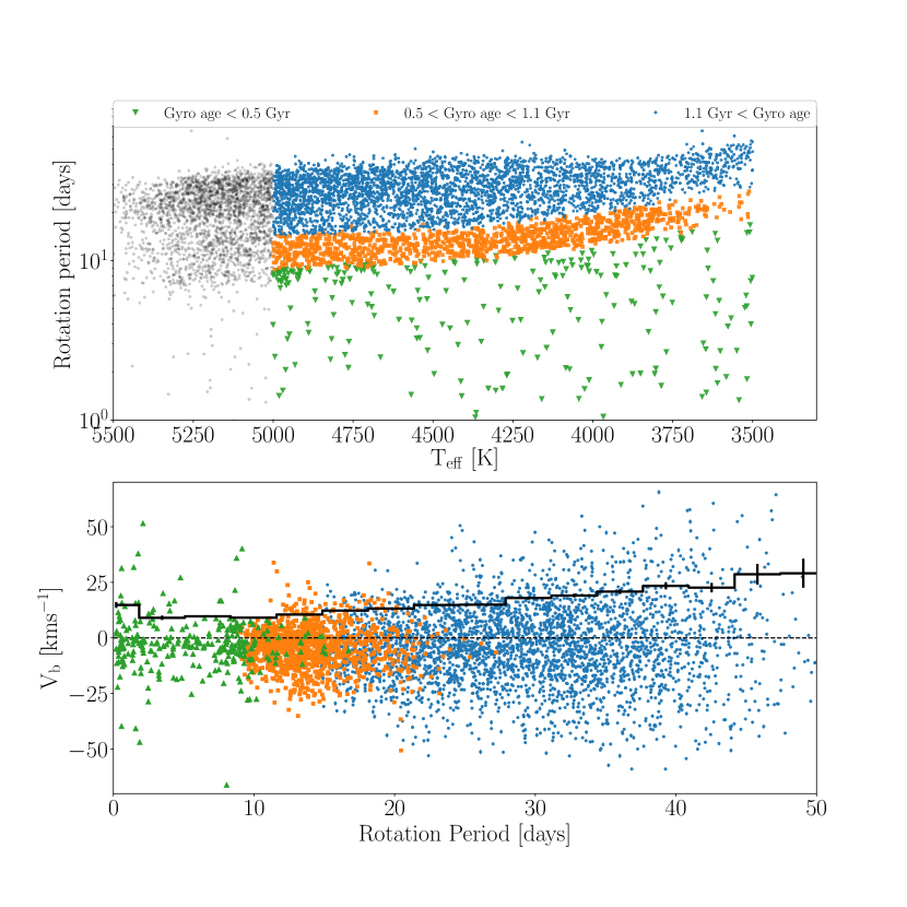
Figure 4: Top: rotation period vs. effective temperature for stars in the McQuillan et al. (2014) sample, separated into three groups. Blue circles show stars with rotation periods longer than the period gap, orange squares show stars with rotation periods shorter than the gap, but longer than the lower edge of the main rotation period distribution, and green triangles show stars with rotation periods shorter than this lower edge. Stars were separated into these three groups using Angus et al. (2019) gyrochronology models, with the scheme shown in the legend. Bottom: the velocities of these groups of stars (in the direction of Galactic latitude, $b$) are shown as a function of rotation period. Only stars cooler than 5000 K are plotted in the bottom panel in order to isolate populations above and below the period gap, which only extends up to temperatures of $\sim$4600 K. The black line indicates the velocity standard deviation as a function of period.

In this section, we explored the kinematic properties of the McQuillan et al. (2014) sample in more detail, investigating the velocity dispersions of stars on either side of the Kepler period gap, and identifying rapidly rotating stars that may be synchronized binaries.

There is a sharp gap in the population of rotation periods (often called the Kepler period gap), which lies just above the 1 Gyr gyrochrone in the upper panel of figure 2, whose origin is unknown and is the subject of much speculation (McQuillan et al., 2014; Davenport, 2017; Davenport & Covey, 2018; Reinhold et al., 2019; Reinhold & Hekker, 2020). This gap was first identified by McQuillan et al. (2014), and roughly follows a line of constant gyrochronal age of around 1.1 Gyr (according to the Angus et al., 2019, gyrochronology relation). Several explanations for the gap’s origin have been proposed, including a discontinuous star formation history (McQuillan et al., 2013; Davenport, 2017; Davenport & Covey, 2018) and a change in magnetic field structure causing a brief period where rotational variability is reduced and rotation periods cannot be measured (Reinhold et al., 2019; Reinhold & Hekker, 2020).

The top panel of figure 2 suggests that the Angus et al. (2019), Praesepe-based gyrochronology model is valid below the gap but not above. Gyrochrones follow lines of constant velocity dispersion below the gap, but cross lines of constant velocity dispersion above the gap. This phenomenon is robust to the choice of bin size and position. Although we do not provide an in-depth analysis here (and more data may be needed to confirm a connection) these data suggest that the gap may indeed separate a young regime where stellar cores are decoupled from their envelopes from an old regime where these layers are more tightly coupled. If so, this could indicate that these phenomena are related, i.e. the process that is responsible for changing the shape of gyrochrones in rotation-$T_{\mathrm{eff}}$ space is related to the process that produces the gap.

An alternate explanation for the gap is that the McQuillan et al. (2014) sample contains two distinct stellar populations: one young and one old. If so, the kinematic properties of stars above and below the gap are likely to be distinctly different. The bottom panel of figure 4 shows the velocity dispersions of stars in the McQuillan et al. (2014) sample, with stars subdivided into three groups: those that rotate more quickly than the main rotation period population (green triangles), those with rotation periods shorter than the gap (orange squares), and those with rotation periods longer than the gap (blue circles). Stars were separated into these three groups using Angus et al. (2019) gyrochronology model, according to the scheme shown in the legend. Only stars cooler than 5000 K are included in the bottom panel in order to isolate populations above and below the period gap, which only extends up to a temperature of $\sim$4600 K in our sample, although Davenport (2017) found that the gap extends to temperatures as hot as 6000 K. In general, velocity dispersion increases with rotation period because both quantities increase with age. Previously, only the overall velocity dispersions of all stars above and below the gap have been compared, leading to the assumption that these groups belong to two distinct populations (McQuillan et al., 2014). However, figure 4 shows a smooth increase in velocity dispersion with rotation period across the gap (from orange squares to blue circles), suggesting that these groups are part of the same Galactic population. This observation does not rule out the possibility that a brief cessation of star formation in the Solar neighborhood, around one Gyr ago, may have caused this gap, however.

In the final part of our analysis, we investigated the potential for using kinematics to identify synchronized binaries in the McQuillan et al. (2014) sample. Synchronized binaries are pairs of stars whose rotation periods are equal to their orbital period. Since synchronization appears to happen at rotation periods of 7 days or shorter (Simonian et al., 2019), and most isolated stars have rotation periods longer than 7 days, the rotation periods of synchronized binaries are likely to be shorter than they would be if they were isolated stars. For this reason, their rotation periods do not reflect their ages and the gyrochronal age of a synchronized binary is likely to be much younger than the true age of the system. Synchronized binaries are therefore a source of contamination for gyrochronology and should be removed from samples before performing a gyrochronal age analysis. Figure 4 shows that some of the most rapidly rotating stars in the McQuillan et al. (2014) sample have relatively large absolute velocities, indicating that they are likely synchronized binaries. For this reason, the velocity dispersions of stars with rotation periods shorter than the lower edge of the rotation period distribution (green triangles in figure 4) are not significantly smaller than the, presumed older, orange-colored stars. In general, stars with rotation periods less than $\sim$10 days have an increased chance of being synchronized binaries. This result is in agreement with a recent study which found that a large fraction of photometric binaries were rapid rotators, and the probability of a star being a synchronized binary system substantially increased below rotation periods of around 7 days (Simonian et al., 2019). We caution users of rotation period catalogs that rapid rotators with large absolute velocities should be flagged as potential synchronized binaries before applying any gyrochronal analysis.

4 Conclusions

In this paper, we used the $v_{\bf b}$ velocity dispersions of stars in the McQuillan et al. (2014) catalog to explore the evolution of stellar rotation period as a function of effective temperature and age. Our conclusions are as follows:

• Spin-down rate doesn’t always increase with decreasing mass for K dwarfs. Although at young ages, rotation period is anti-correlated with $T_{\mathrm{eff}}$ (as seen in many young open clusters, including Praesepe), at intermediate ages the relation flattens out and K dwarfs of different masses rotate at the same rate. At old ages, cooler K dwarfs spin more rapidly than hotter K dwarfs of the same age. While most empirical gyrochronology models calibrated to date can broadly reproduce the rotation periods of young ($\sim$100-700 Gyr) cluster stars, they do not match the rotational behavior of intermediate-age and old ($\gtrsim$1 Gyr) K dwarfs. In addition, their simple functional forms, with a universal age-rotation power-law index, are not flexible enough to capture rotational evolution at all ages and masses. This is because they have been calibrated with young open clusters: stellar spin down is relatively straightforward at young ages, and can often be represented with a color and age-separable power-law relation. Until recently, more complex rotational evolution models were not needed. We now know however, from new observations of intermediate-age clusters, and the kinematic data presented here, that these empirical models are not flexible enough to reproduce the mass and time-dependent spin-down rate of cool dwarfs at old ages. We advocate for the adoption of more flexible models, like semi-parametric Gaussian process models, in the future.

• Variable core-envelope coupling may be the cause. We showed that the period–$T_{\mathrm{eff}}$ relations change shape over time in a way that qualitatively agrees with theoretical models which include mass and time-dependent core-envelope angular momentum transport (Spada & Lanzafame, 2019).

• Low-mass stars stay active longer. We found that the oldest stars in the McQuillan et al. (2014) catalog are cooler than 4500 K, which agrees with previous results which show that lower-mass stars remain active for longer, allowing their rotation periods to be measured at older ages.

• The Kepler period gap may be related to core-envelope coupling. We speculated that the rotation period gap (McQuillan et al., 2014) may separate a young regime where stellar rotation periods decrease with increasing mass from an old regime where periods increase with increasing mass, however more data are needed to provide a conclusive result. The velocity dispersions of stars increase smoothly across the rotation period gap, indicating that the gap does not separate two distinct stellar populations.

• Rapidly rotating stars with large absolute velocities may be synchronized binaries. We used kinematics to indicate that there is a population of synchronized binaries with rotation periods less than around 10 days.

We thank the anonymous referee for their comments which greatly improved this manuscript. We also would like to thank Suzanne Aigrain for providing thoughtful insight that improved the paper. This work was partly developed at the 2019 KITP conference ‘Better stars, better planets’. This research was supported in part by the National Science Foundation under Grant No. NSF PHY-1748958. Parts of this project are based on ideas explored at the Gaia sprints at the Flatiron Institute in New York City, 2016 and MPIA, Heidelberg, 2017. This work made use of the gaia-kepler.fun crossmatch database created by Megan Bedell. T.A.B. acknowledges support by a NASA FINESST award (80NSSC19K1424).

Some of the data presented in this paper were obtained from the Mikulski Archive for Space Telescopes (MAST). STScI is operated by the Association of Universities for Research in Astronomy, Inc., under NASA contract NAS5-26555. Support for MAST for non-HST data is provided by the NASA Office of Space Science via grant NNX09AF08G and by other grants and contracts. This paper includes data collected by the Kepler mission. Funding for the Kepler mission is provided by the NASA Science Mission directorate.

This work has made use of data from the European Space Agency (ESA) mission Gaia (https://www.cosmos.esa.int/gaia), processed by the Gaia Data Processing and Analysis Consortium (DPAC, https://www.cosmos.esa.int/web/gaia/dpac/consortium). Funding for the DPAC has been provided by national institutions, in particular the institutions participating in the Gaia Multilateral Agreement.

5 Appendix A: Validating $v_{\bf b}$ dispersion as an age proxy

The conclusions drawn in this paper depend on the assumption that velocity dispersion in the direction of Galactic latitude ($\sigma_{v{\bf b}}$) can be used as an age proxy. There are two main reasons however, why $v_{\bf b}$ velocity dispersion may not be a good age proxy. Firstly, mass-dependent heating may act on the sample, meaning that velocity dispersion depends on both age and mass. Secondly, since stars in the Kepler field have a range of Galactic latitudes, using $v_{\bf b}$ as a stand-in for $v_{\bf z}$ may not be equally valid for all stars, and introduce a velocity bias for high latitude stars (which are more likely to be cooler and older). In this section we demonstrate that neither of these problems seem to be a significant issue for our data.

In order to establish whether $\sigma_{v{\bf b}}$ can be used as an age proxy, we searched for signs of mass-dependent heating within the Kepler field. Mass-dependent dynamical heating may result from lower-mass stars experiencing greater velocity changes when gravitationally perturbed than more massive stars. It has not been unambiguously observed in the galactic disk because of the strong anti-correlation between stellar mass and stellar age. Less massive stars do indeed have larger velocity dispersions, however they are also older on average. This mass-age degeneracy is highly reduced in M dwarfs because their main-sequence lifetimes are longer than the age of the Universe, and no evidence for mass-dependent heating has previously been found in M dwarfs (e.g. Faherty et al., 2009; Newton et al., 2016).

To investigate whether mass-dependent heating could be acting on the Kepler sample, we selected late K and early M dwarfs observed by both Kepler and Gaia, whose MS lifetimes exceed around 11 Gyr and are therefore representative of the initial mass function. We could not perform this analysis on the McQuillan et al. (2014) sample, because it only includes stars with detectable rotation periods, and since lower-mass stars stay active for longer it is likely that it contains a strong mass-age correlation. We selected all Kepler targets with dereddened Gaia $G_{BP}-G_{RP}$ colors greater than 1.2 (corresponding to an effective temperature $\lesssim$ 4800 K) and absolute Gaia $G$-band magnitudes $>$ 4. We also eliminated photometric binaries by removing stars above a 6th order polynomial, fit to the MS on the Gaia CMD (similar to the one shown in figure 1). We then applied the quality cuts described above in section 2.1. To search for evidence of mass-dependent heating we calculated the ($v_{\bf b}$) velocity dispersion of stars in effective temperature bins. Sigma clipping was performed at 3$\sigma$ to remove high and low velocity outliers before calculating the standard deviation of stars in each bin. These extreme velocity outliers may be very old late K and early M dwarfs, or they result from using $v_{\bf b}$ instead of $v_{\bf z}$, which introduces additional velocity scatter.

Figure 5 shows velocity and velocity dispersion as a function of effective temperature for the K and M Kepler dwarf sample. Velocity dispersion very slightly decreases with decreasing temperature, the opposite of the trend expected for mass-dependent heating, however the slope is only inconsistent with zero at 1.3 $\sigma$. The sharp uptick in velocity dispersion in the coolest bin is probably noise caused by the small number of stars in that bin. This trend may be due to a selection bias: cooler stars are fainter and therefore typically closer, with smaller heights above the galactic plane and smaller velocities. The essential point however, is that we do not see evidence for mass-dependent heating acting on stars in the Kepler field, indicating that velocity dispersion can be used as an age proxy (with the caveat that there is still a chance, albeit a small one, that the opposing effects of the selection function and mass-dependent heating are working to cancel each other out). This analysis was performed using $v_{\bf b}$ but we also examined the vertical velocities of the 537 stars in this sample with RV measurements. Again, no evidence was found for mass-dependent heating: the slope of the velocity dispersion-temperature relation was consistent with zero.

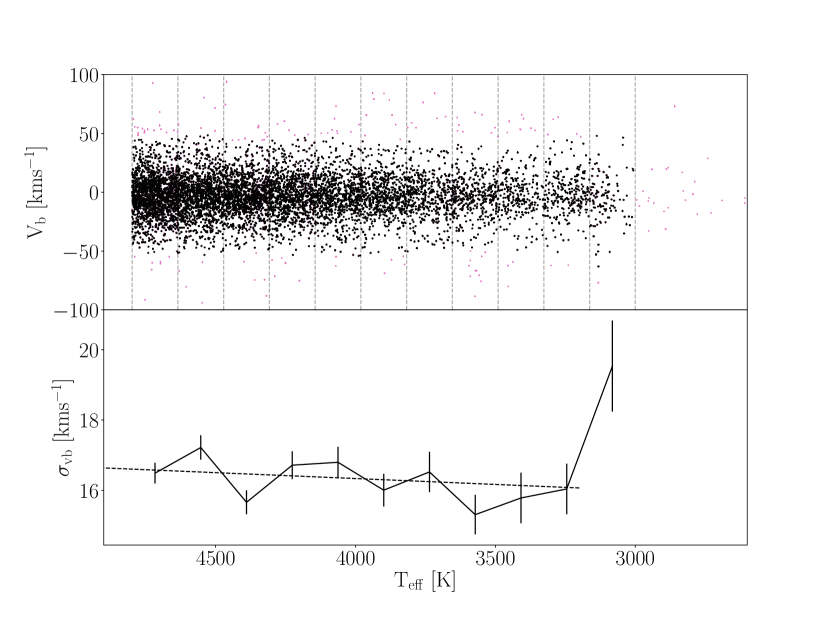
Figure 5: Top: Stellar velocity ($v_{\bf b}$) as a function of $T_{\mathrm{eff}}$ for Kepler K and M dwarfs. Vertical lines indicate different $T_{\mathrm{eff}}$-groupings used to calculate velocity dispersion. Pink stars were not included in velocity dispersion calculations as they were either removed as outliers during a sigma clipping process, or they lie at the sparcely populated, extremely cool end of the temperature range. Velocity dispersion and $T_{\mathrm{eff}}$ are slightly positively correlated, likely due to a brightness-related selection bias, indicating that mass-dependent heating does not significantly affect low-mass stars in the Kepler field.

Having found no strong evidence for mass-dependent heating, we next tested the validity of $v_{\bf b}$ as a proxy for $v_{\bf z}$ in more detail. At a galactic latitude, $b$, of zero, $v_{b}=v_{z}$, however for increasing values of $b$, this equivalence becomes an approximation that grows noisier with $b$. To test the validity of the $v_{\bf b}$$\sim$$v_{\bf z}$ approximation over a range of latitudes we downloaded stellar data from the Gaia Universe Model Snapshot (GUMS) simulation – a simulated Gaia catalog (Robin et al., 2012). We downloaded stars from four pointings in the Kepler field with galactic latitudes of around 5^∘, 10^∘, 15^∘, and 20^∘, out to a limiting magnitude of 16 dex, and calculated their $v_{\bf z}$ and $v_{\bf b}$ velocities. The relationship between $v_{\bf z}$ and $v_{\bf b}$ is close to 1:1, with $v_{\bf z}$ greater than $v_{\bf b}$ by around 4.5 kms^-1 at $b=5$, due to the Sun’s own motion in the Galaxy. We subtracted this offset and examined the residuals of the $v_{\bf z}$ – $v_{\bf b}$ relationship to investigate the variance as a function of Galactic latitude (shown in figure 6). We found that $v_{\bf b}$ is drawn from a heavy-tailed distribution, centered on $v_{\bf z}$, with standard deviation increasing with $b$ (see figure 6). The standard deviation of $v_{\bf z}$-$v_{\bf b}$ was around 3kms^-1 at $b\sim 5^{\circ}$, 4kms^-1 at 10^∘, 6kms^-1 at 15^∘, and 9kms^-1 at 20^∘. This demonstrates that using $v_{\bf b}$ instead of $v_{\bf z}$ for stars in the Kepler field will introduce an additional velocity scatter, inflating $\sigma_{v{\bf b}}$ relative to $\sigma_{v{\bf z}}$. This additional velocity scatter will be greatest for stars at the highest Galactic latitudes.

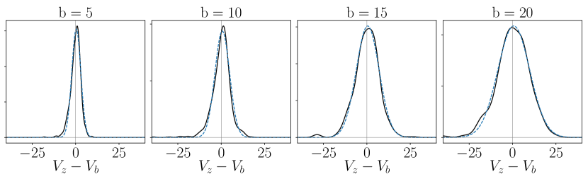
Figure 6: This figure demonstrates the variance in the relationship between $v_{\bf b}$ and $v_{\bf z}$ for stars in the Kepler field, based on the GUMS simulation. The panels show a kernel density estimator (KDE) (black solid line) for the $v_{\bf z}$– $v_{\bf b}$ residuals of stars in the GUMS simulation at four different Galactic latitudes. Blue dashed lines show Gaussian fits to these KDEs. The distributions are close to Gaussian, with slightly heavy tails. The standard deviations of the Gaussian fits increase with Galactic latitude. This figure illustrates how using $v_{\bf b}$ instead of $v_{\bf z}$ artificially increases velocity dispersion, especially at high latitudes.

Since we are concerned with velocity dispersions, rather than velocities themselves, we also compared $\sigma_{v{\bf b}}$ and $\sigma_{v{\bf z}}$ as a function of temperature for stars downloaded from the GUMS simulation. For stars at galactic latitudes of 15^∘ or less, $\sigma_{v{\bf b}}$ was consistent with $\sigma_{v{\bf z}}$, within uncertainties, however, at higher latitudes the two quantities became significantly different. For this reason we proceeded by only including stars with galactic latitudes less than 15^∘ in our analysis. Although we find that the transformation between $v_{\bf z}$ and $v_{\bf b}$ does not strongly affect our results, we cannot rule out the possibility that it introduces systematic biases into the velocity dispersions we present here. In Gaia DR3, RVs will be available for most stars in this sample, providing an opportunity to validate (or correct) the results presented here, and to work in action-space, rather than velocity-space.

Because of the noisy relationship between $v_{\bf b}$ and $v_{\bf z}$  in this paper we do not attempt to convert velocity dispersion ($\sigma_{v{\bf b}}$) into an age via an age-velocity dispersion relation (AVR) (e.g. Holmberg et al., 2009). Although we find that $\sigma_{v{\bf b}}$ can be used to rank populations of stars by age, a more careful analysis that includes formal modeling of the $v_{\bf b}$ – $v_{\bf z}$ relationship will be needed to calculate absolute ages.

6 Appendix B: Photometric temperatures

For this work, we used the precise Gaia DR2 photometric color, $G_{\rm BP}-G_{\rm RP}$, to estimate $T_{\mathrm{eff}}$ for the Kepler rotators. To calibrate this relation, Curtis et al. (2020, submitted) combined effective temperature measurements for nearby, unreddened field stars in benchmark samples, including FGK stars characterized with high-resolution optical spectroscopy (Brewer et al., 2016), M dwarfs characterized with low-resolution optical and near-infrared spectroscopy (Mann et al., 2015), and K and M dwarfs characterized with interferometry and bolometric flux analyses (Boyajian et al., 2012). This empirical color–temperature relation is valid over the color range $0.55<(G_{\rm BP}-G_{\rm RP})_{0}<3.20$, corresponding to $3070<T_{\rm eff}<6470$ K. The dispersion about the relation implies a high precision of 50 K. These benchmark data enable us to accurately estimate $T_{\mathrm{eff}}$ for cool dwarfs (e.g. Rabus et al., 2019), and allows us to correct for interstellar reddening at all temperatures. The equation we used to calculate photometric temperatures from Gaia $G_{BP}-G_{RP}$ color is a seventh-order polynomial with coefficients given in table 1.

Table 1: Coefficient values for the 7th-order polynomial used to estimate $T_{\mathrm{eff}}$ from Gaia $G_{BP}-G_{RP}$ color, calibrated in Curtis et al. (2020, in prep).

($G_{BP}-G_{RP}$ ) exponent	Coefficient
$0$	-416.585
$1$	39780.0
$2$	-84190.5
$3$	85203.9
$4$	-48225.9
$5$	15598.5
$6$	-2694.76
$7$	192.865

2.

Table 2: The data used for this project (the full table is available online). Masses were obtained from Berger et al. (2020), rotation periods from McQuillan et al. (2014), effective temperatures were calculated from dereddened Gaia photometry, as described in the appendix and Curtis et al. (Submitted). Velocities were calculated using pyia and astropy (Astropy Collaboration et al., 2013, 2018; Price-Whelan, 2018). Uncertainties on velocity dispersions were calculated as the standard error of the sample standard deviation (Rao, 1973).

KIC ID	Mass [M⊙]	Teff [K]	Prot [days]	vb [kms-1]	$\sigma_{\mathrm{vb}}$ [kms-1]
1164102	0.63	4053	31.5 $\pm$ 0.5	13.6 $\pm$ 0.2	21.2 $\pm$ 0.4
1292688	0.52	3752	42.7 $\pm$ 2.1	-14.2 $\pm$ 0.2	21.9 $\pm$ 0.7
1297303	0.67	4318	27.3 $\pm$ 0.2	16.7 $\pm$ 0.3	16.7 $\pm$ 0.2
1429921	0.65	4258	23.1 $\pm$ 0.1	-7.0 $\pm$ 0.2	14.8 $\pm$ 0.2
1430349	0.65	4368	34.7 $\pm$ 0.8	12.2 $\pm$ 0.2	19.7 $\pm$ 0.4
1430893	0.61	3985	17.0 $\pm$ 0.0	0.4 $\pm$ 0.1	9.2 $\pm$ 0.1
1431116	0.72	4415	38.8 $\pm$ 1.0	-16.5 $\pm$ 0.1	19.7 $\pm$ 0.4
1432745	0.7	4413	22.2 $\pm$ 0.2	-2.1 $\pm$ 0.0	13.4 $\pm$ 0.2
1435229	0.57	4080	23.5 $\pm$ 0.0	-8.8 $\pm$ 1.0	13.2 $\pm$ 0.2
1569682	0.57	3909	17.4 $\pm$ 0.2	4.4 $\pm$ 0.1	9.2 $\pm$ 0.1

References

- Agüeros et al. (2018) Agüeros, M. A., Bowsher, E. C., & Bochanski et al, J. J. 2018, ApJ, 862, 33, doi: 10.3847/1538-4357/aac6ed
- Angus et al. (2015) Angus, R., Aigrain, S., & Foreman-Mackey et al, D. 2015, MNRAS, 450, 1787, doi: 10.1093/mnras/stv423
- Angus et al. (2019) Angus, R., Morton, T. D., & Foreman-Mackey et al, D. 2019, AJ, 158, 173, doi: 10.3847/1538-3881/ab3c53
- Astropy Collaboration et al. (2013) Astropy Collaboration, Robitaille, T. P., & Tollerud et al, E. J. 2013, A&A, 558, A33, doi: 10.1051/0004-6361/201322068
- Astropy Collaboration et al. (2018) Astropy Collaboration, Price-Whelan, A. M., Sipőcz, B. M., et al. 2018, AJ, 156, 123, doi: 10.3847/1538-3881/aabc4f
- Aumer et al. (2016) Aumer, M., Binney, J., & Schönrich, R. 2016, MNRAS, 462, 1697, doi: 10.1093/mnras/stw1639
- Aumer & Binney (2009) Aumer, M., & Binney, J. J. 2009, MNRAS, 397, 1286, doi: 10.1111/j.1365-2966.2009.15053.x
- Barnes (2003) Barnes, S. A. 2003, ApJ, 586, 464, doi: 10.1086/367639
- Barnes (2007) —. 2007, ApJ, 669, 1167, doi: 10.1086/519295
- Barnes (2010) —. 2010, ApJ, 722, 222, doi: 10.1088/0004-637X/722/1/222
- Beane et al. (2018) Beane, A., Ness, M. K., & Bedell, M. 2018, ApJ, 867, 31, doi: 10.3847/1538-4357/aae07f
- Berger et al. (2020) Berger, T. A., Huber, D., & van Saders et al, J. L. 2020, arXiv e-prints, arXiv:2001.07737. https://arxiv.org/abs/2001.07737
- Bird et al. (2013) Bird, J. C., Kazantzidis, S., & Weinberg et al, D. H. 2013, ApJ, 773, 43, doi: 10.1088/0004-637X/773/1/43
- Borucki et al. (2010) Borucki, W. J., Koch, D., & Basri et al, G. 2010, Science, 327, 977, doi: 10.1126/science.1185402
- Bouvier (2008) Bouvier, J. 2008, A&A, 489, L53, doi: 10.1051/0004-6361:200810574
- Boyajian et al. (2012) Boyajian, T. S., von Braun, K., & van Belle et al, G. 2012, ApJ, 757, 112, doi: 10.1088/0004-637X/757/2/112
- Brewer et al. (2016) Brewer, J. M., Fischer, D. A., & Valenti et al, J. A. 2016, ApJS, 225, 32, doi: 10.3847/0067-0049/225/2/32
- Brun et al. (2011) Brun, A. S., Miesch, M. S., & Toomre, J. 2011, ApJ, 742, 79, doi: 10.1088/0004-637X/742/2/79
- Casagrande et al. (2011) Casagrande, L., Schönrich, R., & Asplund et al, M. 2011, A&A, 530, A138, doi: 10.1051/0004-6361/201016276
- Charbonneau (2010) Charbonneau, P. 2010, Living Reviews in Solar Physics, 7, 3, doi: 10.12942/lrsp-2010-3
- Charbonneau & MacGregor (1993) Charbonneau, P., & MacGregor, K. B. 1993, ApJ, 417, 762, doi: 10.1086/173357
- Curtis et al. (2019) Curtis, J. L., Agüeros, M. A., & Douglas et al, S. 2019, arXiv e-prints. https://arxiv.org/abs/1905.06869
- Davenport (2017) Davenport, J. R. A. 2017, ApJ, 835, 16, doi: 10.3847/1538-4357/835/1/16
- Davenport & Covey (2018) Davenport, J. R. A., & Covey, K. R. 2018, ApJ, 868, 151, doi: 10.3847/1538-4357/aae842
- Denissenkov et al. (2010) Denissenkov, P. A., Pinsonneault, M., & Terndrup et al, D. M. 2010, ApJ, 716, 1269, doi: 10.1088/0004-637X/716/2/1269
- Douglas et al. (2017) Douglas, S. T., Agüeros, M. A., & Covey et al, K. R. 2017, ApJ, 842, 83, doi: 10.3847/1538-4357/aa6e52
- Douglas et al. (2019) Douglas, S. T., Curtis, J. L., & Agüeros et al, M. A. 2019, ApJ, 879, 100, doi: 10.3847/1538-4357/ab2468
- Endal & Sofia (1981) Endal, A. S., & Sofia, S. 1981, ApJ, 243, 625, doi: 10.1086/158628
- Faherty et al. (2009) Faherty, J. K., Burgasser, A. J., & Cruz et al, K. L. 2009, AJ, 137, 1, doi: 10.1088/0004-6256/137/1/1
- Gallet & Bouvier (2013) Gallet, F., & Bouvier, J. 2013, A&A, 556, A36, doi: 10.1051/0004-6361/201321302
- Gallet & Bouvier (2015) —. 2015, A&A, 577, A98, doi: 10.1051/0004-6361/201525660
- García et al. (2014) García, R. A., Ceillier, T., & Salabert et al, D. 2014, A&A, 572, A34, doi: 10.1051/0004-6361/201423888
- Gizis et al. (2000) Gizis, J. E., Monet, D. G., & Reid et al. 2000, AJ, 120, 1085, doi: 10.1086/301456
- Green (2018) Green, G. 2018, The Journal of Open Source Software, 3, 695, doi: 10.21105/joss.00695
- Holmberg et al. (2007) Holmberg, J., Nordström, B., & Andersen, J. 2007, A&A, 475, 519, doi: 10.1051/0004-6361:20077221
- Holmberg et al. (2009) —. 2009, A&A, 501, 941, doi: 10.1051/0004-6361/200811191
- Howell et al. (2014) Howell, S. B., Sobeck, C., & Haas et al, M. 2014, PASP, 126, 398, doi: 10.1086/676406
- Irwin & Bouvier (2009) Irwin, J., & Bouvier, J. 2009, in IAU Symposium, Vol. 258, The Ages of Stars, ed. E. E. Mamajek, D. R. Soderblom, & R. F. G. Wyse, 363–374, doi: 10.1017/S1743921309032025
- Irwin et al. (2007) Irwin, J., Hodgkin, S., & Aigrain et al, S. 2007, MNRAS, 377, 741, doi: 10.1111/j.1365-2966.2007.11640.x
- Janes & Hoq (2011) Janes, K. A., & Hoq, S. 2011, AJ, 141, 92, doi: 10.1088/0004-6256/141/3/92
- Kawaler (1988) Kawaler, S. D. 1988, ApJ, 333, 236, doi: 10.1086/166740
- Kiman et al. (2019) Kiman, R., Schmidt, S. J., & Angus et al, R. 2019, AJ, 157, 231, doi: 10.3847/1538-3881/ab1753
- Kraft (1967) Kraft, R. P. 1967, ApJ, 150, 551, doi: 10.1086/149359
- Lanzafame & Spada (2015) Lanzafame, A. C., & Spada, F. 2015, A&A, 584, A30, doi: 10.1051/0004-6361/201526770
- MacGregor & Brenner (1991) MacGregor, K. B., & Brenner, M. 1991, ApJ, 376, 204, doi: 10.1086/170269
- Mamajek & Hillenbrand (2008) Mamajek, E. E., & Hillenbrand, L. A. 2008, ApJ, 687, 1264, doi: 10.1086/591785
- Mann et al. (2015) Mann, A. W., Feiden, G. A., & Gaidos et al, E. 2015, ApJ, 804, 64, doi: 10.1088/0004-637X/804/1/64
- Martig et al. (2014) Martig, M., Minchev, I., & Flynn, C. 2014, MNRAS, 443, 2452, doi: 10.1093/mnras/stu1322
- Matt et al. (2015) Matt, S. P., Brun, A. S., & Baraffe et al, I. 2015, ApJ, 799, L23, doi: 10.1088/2041-8205/799/2/L23
- Matt et al. (2012) Matt, S. P., MacGregor, K. B., & Pinsonneault et al, M. H. 2012, ApJ, 754, L26, doi: 10.1088/2041-8205/754/2/L26
- McQuillan et al. (2013) McQuillan, A., Aigrain, S., & Mazeh, T. 2013, MNRAS, 432, 1203, doi: 10.1093/mnras/stt536
- McQuillan et al. (2014) McQuillan, A., Mazeh, T., & Aigrain, S. 2014, ApJS, 211, 24, doi: 10.1088/0067-0049/211/2/24
- Meibom et al. (2011) Meibom, S., Barnes, S. A., & Latham et al, D. W. 2011, ApJ, 733, L9, doi: 10.1088/2041-8205/733/1/L9
- Meibom et al. (2015) Meibom, S., Barnes, S. A., & Platais et al, I. 2015, Nature, 517, 589, doi: 10.1038/nature14118
- Metcalfe & Egeland (2019) Metcalfe, T. S., & Egeland, R. 2019, ApJ, 871, 39, doi: 10.3847/1538-4357/aaf575
- Newton et al. (2016) Newton, E. R., Irwin, J., & Charbonneau et al, D. 2016, ApJ, 821, 93, doi: 10.3847/0004-637X/821/2/93
- Newton et al. (2017) —. 2017, ApJ, 834, 85, doi: 10.3847/1538-4357/834/1/85
- Newton et al. (2018) Newton, E. R., Mondrik, N., & Irwin et al, J. 2018, AJ, 156, 217, doi: 10.3847/1538-3881/aad73b
- Nordström et al. (2004) Nordström, B., Mayor, M., & Andersen et al, J. 2004, A&A, 418, 989, doi: 10.1051/0004-6361:20035959
- Oglethorpe & Garaud (2013) Oglethorpe, R. L. F., & Garaud, P. 2013, ApJ, 778, 166, doi: 10.1088/0004-637X/778/2/166
- Parker (1970) Parker, E. N. 1970, ApJ, 162, 665, doi: 10.1086/150697
- Pinsonneault et al. (1989) Pinsonneault, M. H., Kawaler, S. D., & Sofia et al, S. 1989, ApJ, 338, 424, doi: 10.1086/167210
- Price-Whelan (2018) Price-Whelan, Adrian, M. 2018, doi: 10.5281/zenodo.1228136
- Rabus et al. (2019) Rabus, M., Lachaume, R., & Jordán et al, A. 2019, MNRAS, 484, 2674, doi: 10.1093/mnras/sty3430
- Rao (1973) Rao, Radhakrishna, C. 1973, John Wiley & Sons, doi: 10.1002/9780470316436
- Rebull et al. (2017) Rebull, L. M., Stauffer, J. R., & Hillenbrand et al, L. A. 2017, ApJ, 839, 92, doi: 10.3847/1538-4357/aa6aa4
- Reid et al. (1995) Reid, I. N., Hawley, S. L., & Gizis, J. E. 1995, AJ, 110, 1838, doi: 10.1086/117655
- Reiners & Basri (2008) Reiners, A., & Basri, G. 2008, ApJ, 684, 1390, doi: 10.1086/590073
- Reiners & Mohanty (2012) Reiners, A., & Mohanty, S. 2012, ApJ, 746, 43, doi: 10.1088/0004-637X/746/1/43
- Reinhold et al. (2019) Reinhold, T., Bell, K. J., & Kuszlewicz et al, J. 2019, A&A, 621, A21, doi: 10.1051/0004-6361/201833754
- Reinhold & Hekker (2020) Reinhold, T., & Hekker, S. 2020, A&A, 635, A43, doi: 10.1051/0004-6361/201936887
- Robin et al. (2012) Robin, A. C., Luri, X., & Reylé et al, C. 2012, A&A, 543, A100, doi: 10.1051/0004-6361/201118646
- Ruediger & Kitchatinov (1996) Ruediger, G., & Kitchatinov, L. L. 1996, ApJ, 466, 1078, doi: 10.1086/177577
- Sandquist et al. (2016) Sandquist, E. L., Jessen-Hansen, J., & Shetrone et al, M. D. 2016, ApJ, 831, 11, doi: 10.3847/0004-637X/831/1/11
- Schatzman (1962) Schatzman, E. 1962, Annales d’Astrophysique, 25, 18
- Schmidt et al. (2007) Schmidt, S. J., Cruz, K. L., & Bongiorno et al. 2007, AJ, 133, 2258, doi: 10.1086/512158
- Sellwood (2014) Sellwood, J. A. 2014, Reviews of Modern Physics, 86, 1, doi: 10.1103/RevModPhys.86.1
- Simonian et al. (2019) Simonian, G. V. A., Pinsonneault, M. H., & Terndrup, D. M. 2019, ApJ, 871, 174, doi: 10.3847/1538-4357/aaf97c
- Skumanich (1972) Skumanich, A. 1972, ApJ, 171, 565, doi: 10.1086/151310
- Somers & Pinsonneault (2016) Somers, G., & Pinsonneault, M. H. 2016, ApJ, 829, 32, doi: 10.3847/0004-637X/829/1/32
- Spada & Lanzafame (2019) Spada, F., & Lanzafame, A. C. 2019, arXiv e-prints, arXiv:1908.00345. https://arxiv.org/abs/1908.00345
- Spada et al. (2010) Spada, F., Lanzafame, A. C., & Lanza, A. F. 2010, MNRAS, 404, 641, doi: 10.1111/j.1365-2966.2010.16325.x
- Spada et al. (2011) Spada, F., Lanzafame, A. C., & Lanza et al, A. F. 2011, MNRAS, 416, 447, doi: 10.1111/j.1365-2966.2011.19052.x
- Spruit (2002) Spruit, H. C. 2002, A&A, 381, 923, doi: 10.1051/0004-6361:20011465
- Stark & Brand (1989) Stark, A. A., & Brand, J. 1989, ApJ, 339, 763, doi: 10.1086/167334
- Stark & Lee (2005) Stark, A. A., & Lee, Y. 2005, ApJ, 619, L159, doi: 10.1086/427936
- Talon & Charbonnel (2003) Talon, S., & Charbonnel, C. 2003, A&A, 405, 1025, doi: 10.1051/0004-6361:20030672
- Thompson et al. (1996) Thompson, M. J., Toomre, J., & Anderson et al, E. R. 1996, Science, 272, 1300, doi: 10.1126/science.272.5266.1300
- Ting & Rix (2019) Ting, Y.-S., & Rix, H.-W. 2019, ApJ, 878, 21, doi: 10.3847/1538-4357/ab1ea5
- van Saders et al. (2016) van Saders, J. L., Ceillier, T., & Metcalfe et al, T. S. 2016, Nature, 529, 181, doi: 10.1038/nature16168
- van Saders et al. (2018) van Saders, J. L., Pinsonneault, M. H., & Barbieri, M. 2018, ArXiv e-prints. https://arxiv.org/abs/1803.04971
- Weber & Davis (1967) Weber, E. J., & Davis, Jr., L. 1967, ApJ, 148, 217, doi: 10.1086/149138
- West et al. (2006) West, A. A., Bochanski, J. J., & Hawley et al, S. L. 2006, AJ, 132, 2507, doi: 10.1086/508652
- West et al. (2008) West, A. A., Hawley, S. L., & Bochanski et al, J. J. 2008, AJ, 135, 785, doi: 10.1088/0004-6256/135/3/785
- West et al. (2009) West, A. A., Hawley, S. L., & Bochanski et al., J. J. 2009, in IAU Symposium, Vol. 258, The Ages of Stars, ed. E. E. Mamajek, D. R. Soderblom, & R. F. G. Wyse, 327–336, doi: 10.1017/S1743921309031986
- West et al. (2004) West, A. A., Hawley, S. L., & Walkowicz et al, L. M. 2004, AJ, 128, 426, doi: 10.1086/421364