$L^{q}$-spectra of measures on planar non-conformal attractors

Abstract

We study the $L^{q}$-spectrum of measures in the plane generated by certain nonlinear maps. In particular we consider attractors of iterated function systems consisting of maps whose components are $C^{1+\alpha}$ and for which the Jacobian is a lower triangular matrix at every point subject to a natural domination condition on the entries. We calculate the $L^{q}$-spectrum of Bernoulli measures supported on such sets by using an appropriately defined analogue of the singular value function and an appropriate pressure function.

Mathematics Subject Classification 2020: primary: 28A80, 37C45, secondary: 15A18.

Key words and phrases: $L^{q}$-spectrum, generalised $q$-dimensions, non-conformal attractor, modified singular value function, self-affine measure.

1 Introduction

The study of fractals generated by iterated function systems (IFSs) consisting of nonlinear maps, which can often be identified with repellers of corresponding dynamical systems, has a rich history. In 1994 Falconer [5] calculated the dimension of mixing repellers for non-conformal mappings. To do this he applied techniques from thermodynamic formalism, in particular developing a subadditive version of the theory and also a “bounded distortion” principle. Further work on nonlinear IFSs was done by Hu who in 1996 calculated the box and Hausdorff dimensions of invariant sets of expanding $C^{2}$ maps [13]. More recently Cao, Pesin and Zhao [4] studied the Hausdorff dimension of non-conformal repellers corresponding to $C^{1+\alpha}$ maps. By studying certain subadditive and superadditive pressures they were able to obtain bounds for the Hausdorff dimension of repellers.

Other notable work in this area was done in 2007 by Manning and Simon [16] who investigated the subadditive pressure of nonlinear maps developed by Falconer applied to nonlinear maps and considered cases where bounded distortion does not hold. The work of Falconer as well as that of Manning and Simon and also Miao [10] was generalised by Barany [1] who used the subadditive pressure to calculate the Hausdorff dimension of fractals generated by IFSs whose maps have triangular Jacobians. Other authors to have considered IFSs generated by triangular mappings include Kolossváry and Simon [15]. In particular they looked at a family of planar self-affine carpets with overlaps generated by lower triangular matrices and considered whether dimension drop occurs.

In terms of multifractal analysis Falconer studied the $L^{q}$-spectrum of self-affine measures [7] and almost self-affine measures [8]. In the case of self-affine measures he was able to establish a generic formula in the region $1<q\leq 2$ in terms of a subadditive pressure expession. Barral and Feng [2] then generalised this in certain cases to calculate the $L^{q}$-spectrum for a wider range of $q$ and were also able to verify the multifractal formalism in some cases. For results on the $L^{q}$-spectrum of measures on self-affine carpets, see Feng and Wang [11] and Fraser [12].

In this paper we calculate the $L^{q}$-spectra of Bernoulli measures in the plane supported on sets generated by IFSs consisting of $C^{1+\alpha}$ maps whose Jacobian matrices are lower triangular. Our approach is based on setting up certain ‘almost-additive’ pressure functionals. As a corollary we calculate the box dimension of the supports of these measures. Our results on $L^{q}$-dimensions are new, even in the (non-diagonal) self-affine case.

Standard background on iterated function systems may be found, for example, in [9, 14]. We introduce further definitions, in particular nonlinear attractors and nonlinear measures which have a particular meaning in this paper as shorthand for the types of non-conformal attractors and measures we consider.

Definition 1.1 (Nonlinear attractor).

Let $\mathcal{I}$ be a finite index set with $|\mathcal{I}|\geq 2$ and let $\{S_{i}\}_{i\in\mathcal{I}}$ be an IFS consisting of contractions on $[0,1]^{2}$. Suppose also that each $S_{i}:[0,1]^{2}\rightarrow[0,1]^{2}$ is of the form $S_{i}(a_{1},a_{2})=(f_{i}(a_{1}),g_{i}(a_{1},a_{2}))$, where the $f_{i}$ and $g_{i}$ are $C^{1+\alpha}$ contractions ($0<\alpha\leq 1$) on $[0,1]$ and $[0,1]^{2}$ respectively, that is their derivatives satisfy Hölder conditions of exponent $\alpha$. (We use one-sided derivatives on the boundary of $[0,1]^{2}$.) By Hutchinson’s theorem [14] there is a unique non-empty, compact set $F$ satisfying

$$F=\bigcup_{i\in\mathcal{I}}S_{i}(F)$$

which for the purposes of this paper we call the nonlinear attractor associated to $\{S_{i}\}_{i\in\mathcal{I}}$.

We are interested in the natural Bernoulli measures supported on nonlinear attractors $F$, see [6, 14].

Definition 1.2 (Nonlinear measure).

Let $F$ be a nonlinear attractor given by $\{S_{i}\}_{i\in\mathcal{I}}$ on $[0,1]^{2}$, and let $\{p_{i}\}_{i\in\mathcal{I}}$ be a probability vector with each $p_{i}\in(0,1)$. Then there is a unique Borel probability measure $\mu$ supported on $F$ which satisfies

$$\mu=\sum_{i\in\mathcal{I}}p_{i}\ \mu\circ S_{i}^{-1}$$

which we call the nonlinear measure associated to $\{S_{i}\}_{i\in\mathcal{I}}$ and $\{p_{i}\}_{i\in\mathcal{I}}$.

Our aim is to calculate the $L^{q}$-spectra of these measures. Let $\delta>0$ and write $\mathcal{D}_{\delta}$ to denote the set of closed cubes in the $\delta$-mesh on $\mathbb{R}^{n}$ that have positive $\mu$-measure. Write

$$\mathcal{D}^{q}_{\delta}(\mu)=\sum_{Q\in\mathcal{D}_{\delta}}\mu(Q)^{q}.$$ (1.1)

Definition 1.3.

If $\mu$ is a compactly supported Borel probability measure on $\mathbb{R}^{n}$ then for $q\geq 0$ the upper and lower $L^{q}$-spectrum of $\mu$ are defined to be

$$\overline{\tau}_{\mu}(q)=\overline{\lim}_{\delta\rightarrow 0}\frac{\log\mathcal{D}^{q}_{\delta}(\mu)}{-\log\delta}$$ (1.2)

and

$$\underline{\tau}_{\mu}(q)=\underline{\lim}_{\delta\rightarrow 0}\frac{\log\mathcal{D}^{q}_{\delta}(\mu)}{-\log\delta}$$ (1.3)

respectively. If these values coincide then define the $L^{q}$-spectrum of $\mu$, denoted by $\tau_{\mu}(q)$, to be their common value.

The $L^{q}$-spectrum can be thought of as an analogue of box-counting dimension for measures; indeed the upper and lower box dimensions of the support of $\mu$ are easily seen to be given by $\overline{\tau}_{\mu}(0)$ and $\underline{\tau}_{\mu}(0)$ respectively. Note that $\tau_{\mu}(1)=0$ (as $\mu$ is a probability measure) and that $\tau_{\mu}$ is decreasing in $q$. Furthermore the $L^{q}$-spectrum is central in multifractal analysis: in certain key cases the fine multifractal spectrum of $\mu$ can be obtained by taking the Legendre transform of $\tau_{\mu}$ in which case we say that the multifractal formalism holds (see for instance [9, 18]). Another useful property of the $L^{q}$-spectrum is that if it is differentiable at $1$ then the Hausdorff dimension of the measure $\mu$ is given by $\dim_{H}\mu=-\tau_{\mu}^{\prime}(1)$ [17].

For our calculations of $L^{q}$-spectra for nonlinear measures we require the following separation condition for the IFS.

Definition 1.4 (Rectangular open set condition).

An IFS on $\mathbb{R}^{2}$ satisfies the rectangular open set condition (ROSC) if $\{S_{i}((0,1)^{2})\}_{i\in\mathcal{I}}$ are pairwise disjoint subsets of the open unit square $(0,1)^{2}$.

Fraser [12] calculated the $L^{q}$-spectrum $\tau_{\mu}(q)$ of a class of self-affine measures in the plane. We broadly follow his approach although there are several technical challenges which arise due to the nonlinearity, as well as the maps giving rise to non-diagonal Jacobians.

Our main result Theorem 3.8 requires some more assumptions and technical details, in particular that the $\{S_{i}\}_{i\in\mathcal{I}}$ contract more in the vertical direction than in the horizontal direction. The theorem is stated fully in Section 3 but the essence of it is captured in the following version.

Theorem 1.5.

Let $\mu$ be a nonlinear measure which satisfies a natural domination condition and the ROSC and let $q\geq 0$. Then there exists a function $\gamma:[0,\infty)\rightarrow\mathbb{R}$, defined in terms of the probability vector $\{p_{i}\}_{i\in\mathcal{I}}$, the singular values of Jacobian matrices of iterates of the $\{S_{i}\}_{i\in\mathcal{I}}$ and the $L^{q}$-spectrum of the projection of $\mu$ onto the $x$-axis, such that

$$\tau_{\mu}(q)=\gamma(q).$$

We set up the pressure formalism that enables us to define $\gamma$ in Section 3 and prove the theorem in Section 4. A simple corollary is that if $\mu$ satisfies the ROSC then the box dimension of the support of $\mu$ is given by $\gamma(0)$.

2 An Example

Here we provide an example of a nonlinear IFS and corresponding nonlinear attractor generated by three maps. The maps are

$$S_{1}(x,y)=\left(\frac{3x}{5}+\frac{3x^{2}}{40},\ \frac{x^{2}}{12}+\frac{y}{6}\right),$$

$$S_{2}(x,y)=\left(\frac{4x}{5}-\frac{4x^{3}}{30}+\frac{1}{3},\ \frac{x^{2}}{10}+\frac{y}{4}+\frac{17}{50}\right),$$

$$S_{3}(x,y)=\left(\frac{3x}{5},\ \frac{x^{2}}{10}+\frac{y}{5}+\frac{y^{3}}{9}+\frac{26}{45}\right).$$

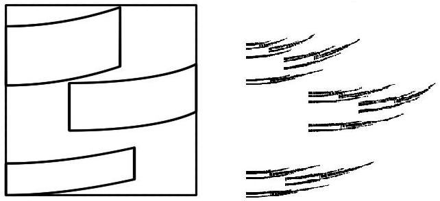
Figure 1: The image of the unit square $[0,1]^{2}$ under the maps $S_{1},S_{2}$ and $S_{3}$ is shown on the left; the IFS satisfies the ROSC (1.4). On the right is the corresponding nonlinear attractor.

These maps satisfy the conditions for Theorem 1.5 and Theorem 3.8. The ROSC and domination condition (3.1) (stated formally in Section 3) are easy to check. Indeed using Maple software gives

$$\inf_{\textbf{a}\in[0,1]^{2}}f_{1,x}(\textbf{a})=3/5>\sup_{\textbf{a}\in[0,1]^{2}}g_{1,y}(\textbf{a})=1/6\geq\inf_{\textbf{a}\in[0,1]^{2}}g_{1,y}(\textbf{a})=1/6$$

$$\inf_{\textbf{a}\in[0,1]^{2}}f_{2,x}(\textbf{a})=2/5>\sup_{\textbf{a}\in[0,1]^{2}}g_{2,y}(\textbf{a})=1/4\geq\inf_{\textbf{a}\in[0,1]^{2}}g_{2,y}(\textbf{a})=1/4$$

$$\inf_{\textbf{a}\in[0,1]^{2}}f_{3,x}(\textbf{a})=3/5>\sup_{\textbf{a}\in[0,1]^{2}}g_{3,y}(\textbf{a})=8/15\geq\inf_{\textbf{a}\in[0,1]^{2}}g_{3,y}(\textbf{a})=1/5$$

with $d=1/6$, say. Thus any nonlinear measures supported on the attractor of this IFS would fall under the class considered.

3 A singular value function and pressure

In [12] Fraser introduced a q-modified singular value function. As he was dealing with self-affine measures he needed to consider the singular values of the linear part of each affine map in the IFS. In our nonlinear setting we shall instead consider singular values of Jacobian matrices.

Let $\{S_{i}\}_{i\in\mathcal{I}}$ be an iterated function system of the form in Definition 1.1. For $\textbf{a}=(a_{1},a_{2})\in[0,1]^{2}$ and $i\in\mathcal{I}$ we denote the derivative of $S_{i}$ by $D_{\textbf{a}}S_{i}$. Note that as each $S_{i}$ is of the form $S_{i}(a_{1},a_{2})=(f_{i}(a_{1}),g_{i}(a_{1},a_{2}))$ the Jacobian matrix of $D_{\textbf{a}}S_{i}$ is a lower triangular matrix. To simplify notation we will write $S_{i}(\textbf{a})=(f_{i}(\textbf{a}),g_{i}(\textbf{a}))$, where $\textbf{a}=(a_{1},a_{2})$, even though $f$ does not depend on $a_{2}$. If we now write $f_{x}$ for the derivative of $f$ and $g_{x}$ and $g_{y}$ for the partial derivatives of $g$ then

$$D_{\textbf{a}}S_{i}=\begin{pmatrix}f_{i,x}(\textbf{a})&0\\ g_{i,x}(\textbf{a})&g_{i,y}(\textbf{a})\end{pmatrix}.$$

From now on we assume that the IFS satisfies the following domination condition, which is our key technical assumption.

Definition 3.1 (Domination Condition).

We say the IFS $\{S_{i}\}_{i\in\mathcal{I}}$ satisfies the domination condition if for each map $S_{i}$ the following inequalities on the derivatives hold:

$$\inf_{{\bf a}\in[0,1]^{2}}f_{i,x}({\bf a})>\sup_{{\bf a}\in[0,1]^{2}}g_{i,y}({\bf a})\geq\inf_{{\bf a}\in[0,1]^{2}}g_{i,y}({\bf a})\geq d,$$ (3.1)

where $d>0$.

Let

$$\eta:=\sup_{i\in\mathcal{I},\textbf{a},\textbf{b}\in[0,1]^{2}}\left\{\frac{g_{i,y}(\textbf{a})}{f_{i,x}(\textbf{b})}\right\}<1$$ (3.2)

using (3.1). In the obvious way we will say that $\mu$ and $F$ satisfy the domination condition if their defining IFS does.

There is no requirement on $g_{i,x}$ to be positive; in particular since this allows $g_{i,x}(\textbf{a})=0$ for all a the class of measures we consider includes self-affine measures supported on Bedford-McMullen carpets, as well as measures supported on attractors of nonlinear “diagonal” IFSs.

Let $\mathcal{I}^{*}=\bigcup_{k\geq 1}\mathcal{I}^{k}$ denote the set of all finite sequences with entries in $\mathcal{I}$. For $\mathfrak{i}=(i_{1},\dots,i_{k})\in\mathcal{I}^{k}$ let $S_{\mathfrak{i}}=S_{i_{1}\cdots i_{k}}:=S_{i_{1}}\circ S_{i_{2}}\circ\cdots\circ S_{i_{k}}$ and let $p(\mathfrak{i})=p_{i_{1}}p_{i_{2}}\cdots p_{i_{k}}$.

We write $0<c<1$ for the maximum contraction ratio of the $S_{i}$ so in particular

$$|S_{i_{1}\cdots i_{k}}(\textbf{a})-S_{i_{1}\cdots i_{k}}(\textbf{b})|\leq c^{k}|\textbf{a}-\textbf{b}|\qquad((i_{1},\dots,i_{k})\in\mathcal{I}^{k},\ \textbf{a},\textbf{b}\in[0,1]^{2}).$$ (3.3)

By the chain rule the Jacobian of the composed maps $S_{\mathfrak{i}}$ must be lower triangular, so let $f_{\mathfrak{i},x}(\textbf{a}),g_{\mathfrak{i},x}(\textbf{a}),g_{\mathfrak{i},y}(\textbf{a})$ denote the entries of $D_{\textbf{a}}S_{\mathfrak{i}}$, that is

$$D_{\textbf{a}}S_{\mathfrak{i}}=\begin{pmatrix}f_{\mathfrak{i},x}(\textbf{a})&0\\ g_{\mathfrak{i},x}(\textbf{a})&g_{\mathfrak{i},y}(\textbf{a})\end{pmatrix}.$$ (3.4)

We will show that the domination condition implies that these matrices satisfy a bounded distortion property which will be key in calculating the $L^{q}$-spectra.

For $x,y\in\mathbb{R}^{+}$ we write $x\lesssim y$ to mean that $x\leq Cy$ for some absolute constant $C>0$. If we wish to emphasize that this constant depends on some other parameter, $\theta$ say, we write $x\lesssim_{\theta}y$. If both $x\lesssim y$ and $y\lesssim x$ we write $x\asymp y$. In this case we say that $x$ and $y$ are comparable.

Using the chain rule the diagonal entries of (3.4) can be written in terms of derivatives of the individual $f_{i}$ and $g_{i}$ as follows.

$$f_{\mathfrak{i},x}(\textbf{a})=\prod_{j=1}^{k}f_{i_{j},x}(S_{i_{j+1}\cdots i_{k}}\textbf{a}),\quad g_{\mathfrak{i},y}(\textbf{a})=\prod_{j=1}^{k}g_{i_{j},y}(S_{i_{j+1}\cdots i_{k}}\textbf{a}).$$ (3.5)

(Here and elsewhere make the natural convention that $S_{i_{k+1}}S_{i_{k}}$ is the identity.) Note that from (3.2), using these expansions,

$$\frac{g_{\mathfrak{i},y}(\textbf{a})}{f_{\mathfrak{i},x}(\textbf{b})}\ \leq\ \eta^{k}$$ (3.6)

for all $\mathfrak{i}=(i_{1},\dots,i_{k})\in\mathcal{I}^{k}$ and all $\textbf{a},\textbf{b}\in[0,1]^{2}$. For the bottom left term direct expansion or induction gives

$$g_{\mathfrak{i},x}(\textbf{a})=\sum_{j=1}^{k}G_{j}(\textbf{a})$$ (3.7)

where, using the chain rule,

$$G_{j}(\textbf{a}) = g_{i_{1},y}(S_{i_{2}\cdots i_{k}}\textbf{a})\cdots g_{i_{j-1},y}(S_{i_{j}\cdots i_{k}}\textbf{a})g_{i_{j},x}(S_{i_{j+1}\cdots i_{k}}\textbf{a})$$ (3.8)

$$\hskip 99.58464pt\times f_{i_{j+1},x}(S_{i_{j+2}\cdots i_{k}}\textbf{a})\cdots f_{i_{k-1},x}(S_{i_{k}}\textbf{a})f_{i_{k},x}(\textbf{a})$$

$$= \bigg{(}\prod_{l=1}^{j-1}g_{i_{l},y}(S_{i_{l+1}\cdots i_{k}}\textbf{a})\bigg{)}g_{i_{j},x}(S_{i_{j+1}\cdots i_{k}}\textbf{a})\bigg{(}\prod_{l=j+1}^{k}f_{i_{l},x}(S_{i_{l+1}\cdots i_{k}}\textbf{a})\bigg{)}$$ (3.9)

$$= g_{i_{1}\cdots i_{j-1},y}(S_{i_{j}\cdots i_{k}}\textbf{a})g_{i_{j},x}(S_{i_{j+1}\cdots i_{k}}\textbf{a})f_{i_{j+1}\cdots i_{k},x}(S_{i_{j+2}\cdots i_{k}}\textbf{a}).$$ (3.10)

The next two lemmas obtain estimates on the entries of (3.4) that are uniform in $\mathfrak{i}$ and a.

Lemma 3.2.

There exists a constant $R>0$ such that for all $\mathfrak{i}\in\mathcal{I}^{*}$ and all ${\bf a},{\bf b}\in[0,1]^{2}$,

$$R^{-1}\ \leq\ \frac{f_{\mathfrak{i},x}({\bf a})}{f_{\mathfrak{i},x}({\bf b})},\ \frac{g_{\mathfrak{i},y}({\bf a})}{g_{\mathfrak{i},y}({\bf b})}\ \leq\ R.$$ (3.11)

Proof.

Note that since each $f_{i_{j}}$ is a $C^{1+\alpha}$ map there is a number $B$ such that

$$|f_{i,x}(\textbf{a}^{\prime})-f_{i,x}(\textbf{b}^{\prime})|\leq B|\textbf{a}^{\prime}-\textbf{b}^{\prime}|^{\alpha}$$

for all $i\in\mathcal{I}$ and all $\textbf{a}^{\prime},\textbf{b}^{\prime}\in[0,1]^{2}$. For $\mathfrak{i}=(i_{1},\dots,i_{k})\in\mathcal{I}^{k}$ and $\textbf{a},\textbf{b}\in[0,1]^{2}$, identity (3.5) gives

$$\frac{f_{\mathfrak{i},x}(\textbf{a})}{f_{\mathfrak{i},x}(\textbf{b})} = \prod_{j=1}^{k}\frac{f_{i_{j},x}(S_{i_{j+1}\cdots i_{k}}\textbf{a})}{f_{i_{j},x}(S_{i_{j+1}\cdots i_{k}}\textbf{b})}$$

$$= \prod_{j=1}^{k}\bigg{(}1+\frac{f_{i_{j},x}(S_{i_{j+1}\cdots i_{k}}\textbf{a})-f_{i_{j},x}(S_{i_{j+1}\cdots i_{k}}\textbf{b})}{f_{i_{j},x}(S_{i_{j+1}\cdots i_{k}}\textbf{b})}\bigg{)}$$

$$\leq \prod_{j=1}^{k}\bigg{(}1+\frac{B|S_{i_{j+1}\cdots i_{k}}\textbf{a}-S_{i_{j+1}\cdots i_{k}}\textbf{b}|^{\alpha}}{d}\bigg{)}$$

$$\leq \prod_{j=1}^{k}\bigg{(}1+\frac{B\,c^{(k-j)\alpha}\,|\textbf{a}-\textbf{b}|^{\alpha}}{d}\bigg{)}$$

$$\leq \prod_{j=1}^{k}\exp\Big{(}\frac{2^{\alpha}B}{d}c^{(k-j)\alpha}\Big{)}$$

$$\leq \exp\sum_{j=1}^{k}\Big{(}\frac{2^{\alpha}B}{d}c^{(k-j)\alpha}\Big{)}$$

$$\leq \exp\Big{(}\frac{2^{\alpha}B}{d(1-c^{\alpha})}\Big{)}$$

using that $|\textbf{a}-\textbf{b}|\leq 2$. Setting $R=\exp({2^{\alpha}B/d(1-c^{\alpha})})$ gives (3.11) for $f_{\mathfrak{i},x}$, with the left-hand estimate obtained by reversing the roles of a and b. A similar argument using (3.5) applies for $g_{\mathfrak{i},y}$. ∎

We turn to the bottom left entries $g_{\mathfrak{i},x}$.

Lemma 3.3.

There exists $C>0$ such that for all $\mathfrak{i}\in\mathcal{I}^{*}$ and all ${\bf a},{\bf b}\in[0,1]^{2}$

$$\bigg{|}\frac{g_{\mathfrak{i},x}({\bf a})}{f_{\mathfrak{i},x}({\bf b})}\bigg{|}\leq C.$$ (3.13)

Proof.

Let $\mathfrak{i}=(i_{1},\dots,i_{k})\in\mathcal{I}^{k}$ and $\textbf{a},\textbf{b}\in[0,1]^{2}$. Then for $1\leq j\leq k$ identities (3.5) and (3.9) give

$$\bigg{|}\frac{G_{j}(\textbf{a})}{f_{\mathfrak{i},x}(\textbf{b})}\bigg{|} = \bigg{|}\bigg{(}\prod_{l=1}^{j-1}\frac{g_{i_{l},y}(S_{i_{l+1}\cdots i_{k}}\textbf{a})}{f_{i_{l},x}(S_{i_{l+1}\cdots i_{k}}\textbf{b})}\bigg{)}\frac{g_{i_{j},x}(S_{i_{j+1}\cdots i_{k}}\textbf{a})}{f_{i_{j},x}(S_{i_{j+1}\cdots i_{k}}\textbf{b})}\bigg{(}\prod_{l=j+1}^{k}\frac{f_{i_{l},x}(S_{i_{l+1}\cdots i_{k}}\textbf{a})}{f_{i_{l},x}(S_{i_{l+1}\cdots i_{k}}\textbf{b})}\bigg{)}\bigg{|}$$

$$= \bigg{(}\prod_{l=1}^{j-1}\bigg{|}\frac{g_{i_{l},y}(S_{i_{l+1}\cdots i_{k}}\textbf{a})}{f_{i_{l},x}(S_{i_{l+1}\cdots i_{k}}\textbf{b})}\bigg{|}\bigg{)}\bigg{|}\frac{g_{i_{j},x}(S_{i_{j+1}\cdots i_{k}}\textbf{a})}{f_{i_{j},x}(S_{i_{j+1}\cdots i_{k}}\textbf{b})}\bigg{|}\bigg{|}\frac{f_{i_{j+1}\cdots i_{k},x}(\textbf{a})}{f_{i_{j+1}\cdots i_{k},x}(\textbf{b})}\bigg{|}$$

$$\leq \eta^{j-1}\eta R,$$

using (3.2) and where $R$ is as in (3.11). Hence by (3.7)

$$\bigg{|}\frac{g_{\mathfrak{i},x}(\textbf{a})}{f_{\mathfrak{i},x}(\textbf{b})}\bigg{|}\ =\ \bigg{|}\frac{\sum_{j=1}^{k}G_{j}(\textbf{a})}{f_{\mathfrak{i},x}(\textbf{b})}\bigg{|}\ \leq\ \sum_{j=1}^{k}\bigg{|}\frac{G_{j}(\textbf{a})}{f_{\mathfrak{i},x}(\textbf{b})}\bigg{|}\ \leq\ \sum_{j=1}^{k}R\,\eta^{j}\ <\ \frac{R\,\eta}{1-\eta},$$

giving (3.13) with $C=R\eta/(1-\eta)$. ∎

Recall that the singular values of an $n\times n$ matrix $A$ are defined to be the eigenvalues of $A^{T}A$. For $\textbf{a}=(a_{1},a_{2})\in[0,1]^{2}$ write $\alpha_{1}(D_{\textbf{a}}S_{\mathfrak{i}})\geq\alpha_{2}(D_{\textbf{a}}S_{\mathfrak{i}})$ for the singular values of $D_{\textbf{a}}S_{\mathfrak{i}}$.

Lemma 3.4.

The singular values of the Jacobian matrices $D_{{\bf a}}S_{\mathfrak{i}}$ satisfy

$$\alpha_{1}(D_{{\bf a}}S_{\mathfrak{i}})\asymp f_{\mathfrak{i},x}({\bf a})$$ (3.14)

and

$$\alpha_{2}(D_{{\bf a}}S_{\mathfrak{i}})\asymp g_{\mathfrak{i},y}({\bf a})$$ (3.15)

for all ${\bf a}\in[0,1]^{2}$ and $\mathfrak{i}\in\mathcal{I}^{*}$.

Proof.

Let

$$A=\begin{pmatrix}a&0\\ b&c\end{pmatrix}.$$

be a matrix with $0\leq c\leq a$ and $0\leq b\leq Ca$ for some constant $C>0$. Calculating the larger singular value $\alpha_{1}(A)$ of $A$, which is the (positive) square root of the larger eigenvalue of $AA^{T}$,

$$\alpha_{1}(A)^{2}={\textstyle\frac{1}{2}}\Big{(}(a^{2}+b^{2}+c^{2})+\big{(}(a^{2}+b^{2}+c^{2})^{2}-4a^{2}c^{2}\big{)}^{1/2}\Big{)}.$$

Making obvious estimates,

$${\textstyle\frac{1}{2}}a^{2}\ \leq\ \alpha_{1}(A)^{2}\ \leq\ a^{2}+b^{2}+c^{2}\ \leq\ (2+C^{2})a^{2}.$$

Applying this to the matrix

$$D_{\textbf{a}}S_{\mathfrak{i}}=\begin{pmatrix}f_{\mathfrak{i},x}(\textbf{a})&0\\ g_{\mathfrak{i},x}(\textbf{a})&g_{\mathfrak{i},y}(\textbf{a})\end{pmatrix},$$

where $0\leq g_{\mathfrak{i},y}(\textbf{a})\leq f_{\mathfrak{i},x}(\textbf{a})$ by (3.6) and $0\leq|g_{\mathfrak{i},x}(\textbf{a})|\leq Cf_{\mathfrak{i},x}(\textbf{a})$ by (3.13), gives (3.14). Using that $\alpha_{1}(A)\alpha_{2}(A)=\det A=ac$ for the matrix $A$, (3.15) follows immediately from (3.14). ∎

A immediate consequence of Lemmas 3.2 and 3.4 is that the singular values of the Jacobian matrices satisfy

$$\alpha_{1}(D_{\textbf{a}}S_{\mathfrak{i}})\asymp\alpha_{1}(D_{\textbf{b}}S_{\mathfrak{i}})\quad\mbox{ and }\quad\alpha_{2}(D_{\textbf{a}}S_{\mathfrak{i}})\asymp\alpha_{2}(D_{\textbf{b}}S_{\mathfrak{i}})$$ (3.16)

for all $\textbf{a},\textbf{b}\in[0,1]^{2}$ and $\mathfrak{i}\in\mathcal{I}^{*}$.

We define the projection map onto the $x$-axis $\pi:\mathbb{R}^{2}\rightarrow\mathbb{R}$ by $\pi(x,y)=x$. It is immediate that the projection of the nonlinear measure $\mu$ onto the $x$-axis, $\pi(\mu)$, is a self-conformal measure. It follows from a result of Peres and Solomyak [19] that the $L^{q}$-spectra of this projected measure, which we denote by

$$\beta(q):=\tau_{\pi(\mu)}(q),$$ (3.17)

exists for $q\geq 0$. Note that this holds even if there are complicated overlaps between the components of the projected measure, which is the typical situation for us.

For $s\in\mathbb{R}$, $q\geq 0$ and $\textbf{a}\in[0,1]^{2}$, we define the q-modified singular value function, $\psi^{s,q}_{\textbf{a}}:\mathcal{I}^{*}\rightarrow(0,\infty)$ by

$$\psi^{s,q}_{\textbf{a}}(\mathfrak{i})=p(\mathfrak{i})^{q}\alpha_{1}(D_{\textbf{a}}S_{\mathfrak{i}})^{\beta(q)}\alpha_{2}(D_{\textbf{a}}S_{\mathfrak{i}})^{s-\beta(q)}.$$ (3.18)

It follows from (3.16) that for all $\textbf{a},\textbf{b}\in[0,1]^{2}$ and $\mathfrak{i}\in\mathcal{I}^{*}$ we have $\psi^{s,q}_{\textbf{a}}(\mathfrak{i})\asymp_{s,q}\psi^{s,q}_{\textbf{b}}(\mathfrak{i})$. Moreover, by Lemma 3.2,

$$\psi^{s,q}_{\textbf{a}}(\mathfrak{i})\asymp_{s,q}p(\mathfrak{i})^{q}f_{\mathfrak{i},x}(\textbf{a})^{\beta(q)}g_{\mathfrak{i},y}(\textbf{a})^{s-\beta(q)}.$$ (3.19)

For each $k\in\mathbb{N}$ define $\Psi_{\textbf{a},k}^{s,q}$ by

$$\Psi_{\textbf{a},k}^{s,q}=\sum_{\mathfrak{i}\in\mathcal{I}^{k}}\psi^{s,q}_{\textbf{a}}(\mathfrak{i}).$$ (3.20)

The quantities $\psi^{s,q}_{\textbf{a}}(\mathfrak{i})$ and $\Psi_{\textbf{a},k}^{s,q}$ satisfy some useful multiplicative properties, similar to those from [12, Lemma 2.2].

Lemma 3.5.

Let $s\in\mathbb{R}$, $q\geq 0$ and ${\bf a}\in[0,1]^{2}$.

(a) If $\mathfrak{i},\mathfrak{j}\in\mathcal{I}^{*}$ then

$$\psi^{s,q}_{{\bf a}}(\mathfrak{i}\mathfrak{j})\asymp_{s,q}\psi^{s,q}_{{\bf a}}(\mathfrak{i})\psi^{s,q}_{{\bf a}}(\mathfrak{j}).$$ (3.21)

(b) If $k,l\in\mathbb{N}$ then

$$\Psi_{{\bf a},k+l}^{s,q}\asymp_{s,q}\Psi_{{\bf a},k}^{s,q}\Psi_{{\bf a},l}^{s,q}.$$ (3.22)

Proof.

By the chain rule applied to $f_{\mathfrak{ij},x}$ and using (3.11),

$$f_{\mathfrak{ij},x}({\bf a})=f_{\mathfrak{i},x}(S_{\mathfrak{i}}{\bf a})f_{\mathfrak{j},x}({\bf a})\asymp_{s,q}f_{\mathfrak{i},x}({\bf a})f_{\mathfrak{j},x}({\bf a}),$$

and similarly

$$g_{\mathfrak{ij},y}({\bf a})\asymp_{s,q}g_{\mathfrak{i},y}({\bf a})g_{\mathfrak{j},y}({\bf a}).$$

Using the form (3.19)

$$\psi^{s,q}_{\textbf{a}}(\mathfrak{ij}) \asymp_{s,q}p(\mathfrak{ij})^{q}f_{\mathfrak{ij},x}(\textbf{a})^{\beta(q)}g_{\mathfrak{ij},y}(\textbf{a})^{s-\beta(q)}$$

$$\asymp_{s,q}p(\mathfrak{i})^{q}p(\mathfrak{j})^{q}f_{\mathfrak{i},x}(\textbf{a})^{\beta(q)}f_{\mathfrak{j},x}(\textbf{a})^{\beta(q)}g_{\mathfrak{i},y}(\textbf{a})^{s-\beta(q)}g_{\mathfrak{j},y}(\textbf{a})^{s-\beta(q)}$$

$$\asymp_{s,q}\psi^{s,q}_{\textbf{a}}(\mathfrak{i})\psi^{s,q}_{\textbf{a}}(\mathfrak{j})$$

giving (3.21)

For part (b), if $k,l\in\mathbb{N}$ then

$$\Psi_{\textbf{a},k+l}^{s,q}=\sum_{\mathfrak{i}\in\mathcal{I}^{k+l}}\psi^{s,q}_{\textbf{a}}(\mathfrak{i})=\sum_{\mathfrak{i}\in\mathcal{I}^{k}}\sum_{\mathfrak{j}\in\mathcal{I}^{l}}\psi^{s,q}_{\textbf{a}}(\mathfrak{ij})$$

and

$$\Psi_{\textbf{a},k}^{s,q}\Psi_{\textbf{a},l}^{s,q}=\Big{(}\sum_{\mathfrak{i}\in\mathcal{I}^{k}}\psi^{s,q}_{\textbf{a}}(\mathfrak{i})\Big{)}\Big{(}\sum_{\mathfrak{j}\in\mathcal{I}^{l}}\psi^{s,q}_{\textbf{a}}(\mathfrak{j})\Big{)}=\sum_{\mathfrak{i}\in\mathcal{I}^{k}}\sum_{\mathfrak{j}\in\mathcal{I}^{l}}\psi^{s,q}_{\textbf{a}}(\mathfrak{i})\psi^{s,q}_{\textbf{a}}(\mathfrak{j}).$$

Applying part (a) to the double sums completes the proof. ∎

We call a sequence $\{a_{n}\}_{n\in\mathbb{N}}$ with $a_{n}>0$ (such as those in Lemma 3.5) for which there exists an absolute constants $0<K_{1}\leq K_{2}$ such that

$$K_{1}a_{n}a_{m}\leq a_{n+m}\leq K_{2}a_{n}a_{m}$$ (3.23)

for all $n,m\in\mathbb{N}$ almost-multiplicative. For such sequences the limit $\lim_{n\to\infty}a_{n}^{1/n}$ exists, see for example [6, Corollary 1.2].

It follows from Lemma 3.5 that for each $\textbf{a}\in[0,1]^{2}$ we may define a function $P_{\textbf{a}}:\mathbb{R}\times[0,\infty)\rightarrow[0,\infty)$ by

$$P_{\textbf{a}}(s,q)=\lim_{k\rightarrow\infty}(\Psi_{\textbf{a},k}^{s,q})^{1/k}.$$

Note that the value of $P_{\textbf{a}}(s,q)$ is unchanged if we replace the right-hand side of (3.18) by the right-hand side of (3.19) in the definition of $\psi^{s,q}_{\textbf{a}}(\mathfrak{i})$ and thus of $\Psi_{\textbf{a},k}^{s,q}$. Moreover, as $\psi^{s,q}_{\textbf{a}}(\mathfrak{i})\asymp_{s,q}\psi^{s,q}_{\textbf{b}}(\mathfrak{i})$ and thus $\Psi_{\textbf{a},k}^{s,q}\asymp_{s,q}\Psi_{\textbf{b},k}^{s,q}$ for all $\textbf{a},\textbf{b}\in[0,1]^{2}$ it is easy to see that $P_{\textbf{a}}$ is independent of the choice of a. Thus we shall just write $P$ instead of $P_{\textbf{a}}$. For a fixed $q\geq 0$ we think of the function $s\mapsto\log P(s,q)$ as the topological pressure of the system.

We also write the following

$$\alpha_{\textnormal{min}} =\inf\{\alpha_{2}(D_{\textbf{a}}S_{i}):\textbf{a}\in[0,1]^{2},\ i\in\mathcal{I}\},$$

$$\alpha_{\textnormal{max}} =\sup\{\alpha_{1}(D_{\textbf{a}}S_{i}):\textbf{a}\in[0,1]^{2},\ i\in\mathcal{I}\},$$

$$p_{\textnormal{min}} =\textnormal{min}\{p_{i}:i\in\mathcal{I}\},$$

$$p_{\textnormal{max}} =\textnormal{max}\{p_{i}:i\in\mathcal{I}\}$$

and note that $0<\alpha_{\textnormal{min}},\alpha_{\textnormal{max}},p_{\textnormal{min}},p_{\textnormal{max}}<1$.

Recall that the $L^{q}$-spectrum of a given measure is Lipschitz continuous (as it is concave and decreasing) on $[\lambda,\infty)$ for all $\lambda>0$. Let $L_{\lambda}$ denote the Lipschitz constant of $\beta$ on $[\lambda,\infty)$. We can now state some basic properties of $P$.

Lemma 3.6.

(1) For $s,r\in\mathbb{R}$ and $\lambda>0$ define

$$U(s,r,\lambda)=\textnormal{min}\left\{\alpha_{\textnormal{min}}^{s}p_{\textnormal{min}}^{r},\alpha_{\textnormal{min}}^{s}p_{\textnormal{max}}^{r},\alpha_{\textnormal{max}}^{s}p_{\textnormal{min}}^{r},\alpha_{\textnormal{max}}^{s}p_{\textnormal{max}}^{r}\right\}(\alpha_{\textnormal{max}}/\alpha_{\textnormal{min}})^{\textnormal{min}\{-L_{\lambda}r,0\}}$$

and

$$V(s,r,\lambda)=\textnormal{max}\left\{\alpha_{\textnormal{min}}^{s}p_{\textnormal{min}}^{r},\alpha_{\textnormal{min}}^{s}p_{\textnormal{max}}^{r},\alpha_{\textnormal{max}}^{s}p_{\textnormal{min}}^{r},\alpha_{\textnormal{max}}^{s}p_{\textnormal{max}}^{r}\right\}(\alpha_{\textnormal{max}}/\alpha_{\textnormal{min}})^{\textnormal{max}\{-L_{\lambda}r,0\}}.$$

Then for all $s,t\in\mathbb{R},\lambda>0,q\geq\lambda$ and $r\geq\lambda-q$

$$U(s,r,\lambda)P(t,q)\leq P(s+t,q+r)\leq V(s,r,\lambda)P(t,q),$$

and for all $s,t\in\mathbb{R}$

$$\textnormal{min}\left\{\alpha_{\textnormal{min}}^{s},\alpha_{\textnormal{max}}^{s}\right\}P(t,0)\leq P(s+t,0)\leq\textnormal{max}\left\{\alpha_{\textnormal{min}}^{s},\alpha_{\textnormal{max}}^{s}\right\}P(t,0).$$

Also for all $s\in\mathbb{R}$ and $q\geq 0$

$$P(s,q)\leq p_{\textnormal{max}}^{q}P(s,0).$$

(2) $P$ is continuous on $\mathbb{R}\times(0,\infty)$ and on $\mathbb{R}\times\{0\};$

(3) $P$ is strictly decreasing in $s\in\mathbb{R}$ and $q\in(0,\infty);$

(4) For each $q\geq 0$ there exists a unique $s\geq 0$ such that $P(s,q)=1$.

Proof.

This is essentially the same as the proof of the analogous result of Fraser [12, Lemma 2.3] and as such is omitted. ∎

It follows from Lemma 3.6 that we may define a function $\gamma:[0,\infty)\rightarrow\mathbb{R}$ by $P(\gamma(q),q)=1$ which we shall refer to as a moment scaling function. The moment scaling function satisfies the following useful properties.

Lemma 3.7.

(1) $\gamma$ is strictly decreasing on $[0,\infty);$

(2) $\gamma$ is continuous on $(0,\infty);$

(3) $\gamma(1)=0$ and $\lim_{q\rightarrow\infty}\gamma(q)=-\infty;$

(4) $\gamma$ is convex on $(0,\infty)$.

Proof.

This follows by the same reasoning as in the proof of [12, Lemma 2.5]. ∎

We can now state our main theorem which relates $\gamma$ to the $L^{q}$-spectrum $\tau_{\mu}(q)$ of $\mu$.

Theorem 3.8.

Let $\mu$ be a nonlinear measure which satisfies the domination condition (3.1). Then

(1) For $q\in[0,1]$

$$\overline{\tau}_{\mu}(q)\leq\gamma(q);$$

(2) For $q\geq 1$

$$\underline{\tau}_{\mu}(q)\geq\gamma(q);$$

(3) If $\mu$ also satisfies the ROSC then for all $q\geq 0$

$$\tau_{\mu}(q)=\gamma(q).$$

We shall prove this theorem in Section 4.

As a corollary we are able to calculate the box dimension of the support of these measures. We recall the definition of the box dimension.

Definition 3.9.

Let $X\subset\mathbb{R}^{n}$ be bounded and non-empty and let $N_{\delta}(X)$ denote the minimal number of sets of diameter at most $\delta$ needed to cover $X$. The upper and lower box dimension are defined to be

$$\overline{\dim_{B}}X=\overline{\lim}_{\delta\rightarrow 0}\frac{\log N_{\delta}(X)}{-\log\delta}$$

and

$$\underline{\dim_{B}}X=\underline{\lim}_{\delta\rightarrow 0}\frac{\log N_{\delta}(X)}{-\log\delta}$$

respectively. If these numbers coincide then we define the box dimension of $X$, denoted $\dim_{B}X$, to be their common value.

Corollary 3.10.

Let $F$ be a nonlinear attractor which satisfies the domination condition (3.1). Then (1)

$$\overline{\dim_{B}}F\leq\gamma(0);$$

(2) If $F$ also satisfies the ROSC then

$$\dim_{B}F=\gamma(0).$$

Proof.

It is well-known that the upper and lower box dimension of the support of a measure is given by the upper and lower $L^{q}$-spectrum at $0$. The result is then immediate from Theorem 3.8. ∎

Note that $\gamma(0)$ depends on $\beta(0)=\dim_{B}\pi F$, the box dimension of the projection of $F$ onto the $x$-axis. Also note that by standard results, e.g. [9, Corollary 3.10], the packing dimension of a nonlinear attractor coincides with the upper box dimension and so Corollary 3.10 also yields the packing dimension.

4 Calculating the $L^{q}$-spectrum

We begin this section by introducing some notation. For ${\mathfrak{i}}=(i_{1},i_{2},\dots,i_{k})\in\mathcal{I}^{*}$ let $\widehat{\mathfrak{i}}\in\mathcal{I}^{*}\cup\{\omega\}$ be given by

$$\hat{\mathfrak{i}}=(i_{1},i_{2},\dots,i_{k-1})$$

where $\omega$ is the empty word. For $\delta\in(0,1]$ and $\textbf{a}\in[0,1]^{2}$ we define the $\delta$-stopping by

$$\mathcal{I}_{\textbf{a},\delta}=\{\mathfrak{i}\in\mathcal{I}^{*}:\alpha_{2}(D_{\textbf{a}}S_{\mathfrak{i}})<\delta\leq\alpha_{2}(D_{\textbf{a}}S_{\hat{\mathfrak{i}}})\}$$

where $S_{\omega}$ is the identity map. Note that if $\mathfrak{i}\in\mathcal{I}_{\textbf{a},\delta}$ then

$$\alpha_{\textnormal{min}}\delta\leq\alpha_{2}(D_{\textbf{a}}S_{\mathfrak{i}})<\delta.$$ (4.1)

For $\mathfrak{i}\in\mathcal{I}^{*}$ let $\mu_{\mathfrak{i}}=p(\mathfrak{i})\mu\circ S_{\mathfrak{i}}^{-1}$ and $F_{\mathfrak{i}}=S_{\mathfrak{i}}(F)=\textnormal{supp}\mu_{\mathfrak{i}}.$ Note that for all $\textbf{a}\in[0,1]^{2}$ and $\delta\in(0,1]$,

$$\mu=\sum_{\mathfrak{i}\in\mathcal{I}_{\textbf{a},\delta}}\mu_{\mathfrak{i}}.$$

Lemma 4.1.

Let ${\bf a}\in[0,1]^{2}$, $t\in\mathbb{R}$ and $q\geq 0$.

(1) If $t>\gamma(q)$ then

$$\sum_{\mathfrak{i}\in\mathcal{I}_{{\bf a},\delta}}\psi^{t,q}_{{\bf a}}(\mathfrak{i})\lesssim_{t,q}1$$

for all $\delta\in(0,1]$.

(2) If $t<\gamma(q)$ then

$$\sum_{\mathfrak{i}\in\mathcal{I}_{{\bf a},\delta}}\psi^{t,q}_{{\bf a}}(\mathfrak{i})\gtrsim_{t,q}1$$

for all $\delta\in(0,1]$.

Proof.

The proof follows that of [12, Lemma 7.1] which only depends on the multiplicative properties of $\Psi$ (which we have established here) so is omitted. ∎

Our next lemma allows us to control the length of the side of $S_{\mathfrak{i}}([0,1]^{2})$ in terms of the length of its base.

Lemma 4.2.

There exists $L>0$ such that for all $\mathfrak{i}\in\mathcal{I}^{*}$ and all $0\leq a<b\leq 1$

$$\frac{|g_{\mathfrak{i}}(b,1)-g_{\mathfrak{i}}(a,1)|}{|f_{\mathfrak{i}}(b)-f_{\mathfrak{i}}(a)|}\leq L,$$

noting that $f_{\mathfrak{i}}$ depends only on the first coordinate of its argument.

Proof.

By the mean value theorem there exist $c_{1},c_{2}\in(a,b)$ such that

$$\frac{|g_{\mathfrak{i}}(b,1)-g_{\mathfrak{i}}(a,1)|}{|f_{\mathfrak{i}}(b)-f_{\mathfrak{i}}(a)|}=\frac{|g_{\mathfrak{i},x}(c_{1},1)||b-a|}{|f_{\mathfrak{i},x}(c_{2})||b-a|}=\frac{|g_{\mathfrak{i},x}(c_{1},1)|}{|f_{\mathfrak{i},x}(c_{2})|}\lesssim 1$$

by Lemma 3.3. ∎

The standard inequalities, that if $k\in\mathbb{N},a_{1},\dots,a_{k}\geq 0$ and $q\geq 0$ then

$$\left(\sum_{i=1}^{k}a_{i}\right)^{q}\asymp_{k,q}\sum_{i=1}^{k}a_{i}^{q},$$ (4.2)

will be helpful when manipulating moment sums.

Recall from (1.1) that $\mathcal{D}_{\delta}^{q}$ denotes the $q$-th power moment sum of a measure over the $\delta$-mesh cubes $\mathcal{D}_{\delta}$. Our next result compares the moment sums of $\mu_{\mathfrak{i}}=p(\mathfrak{i})\mu\circ S_{\mathfrak{i}}^{-1}$ on $S_{\mathfrak{i}}(F)$ with moment sums of the projection of $\mu$ onto the horizontal axis. This is analogous to [12, Lemma 7.2] but in the nonlinear case more care is needed.

Lemma 4.3.

For each $q\geq 0$ and ${\bf a}\in[0,1]^{2}$, there exist numbers $\widehat{A},\widehat{B}>0$ such that if we write

$$\widehat{A}_{\mathfrak{i},\delta}=\frac{\widehat{A}\delta}{\alpha_{1}(D_{{\bf a}}S_{\mathfrak{i}})}\qquad{\text{a}nd}\qquad\widehat{B}_{\mathfrak{i},\delta}=\frac{\widehat{B}\delta}{\alpha_{1}(D_{{\bf a}}S_{\mathfrak{i}})}$$ (4.3)

for $\delta\in(0,1]$ and $\mathfrak{i}\in\mathcal{I}_{{\bf a},\delta}$ then

$$\mathcal{D}^{q}_{\widehat{B}_{\mathfrak{i},\delta}}(p(\mathfrak{i})\pi\mu)\ \lesssim\ \mathcal{D}^{q}_{\delta}(\mu_{\mathfrak{i}})\ \lesssim\ \mathcal{D}^{q}_{\widehat{A}_{\mathfrak{i},\delta}}(p(\mathfrak{i})\pi\mu).$$ (4.4)

Proof.

As $\mathfrak{i}\in\mathcal{I}_{\textbf{a},\delta}$ we have $\alpha_{2}(D_{\textbf{a}}S_{\mathfrak{i}})<\delta$. We shall show that there are at most a constant number $k$ squares of the $\delta$-mesh that intersect $S_{\mathfrak{i}}([0,1]^{2})\supseteq\textnormal{supp}\mu_{\mathfrak{i}}$ in any vertical column of mesh squares.

For this we estimate the height of the intersection of $S_{\mathfrak{i}}([0,1]^{2})$ with a given vertical strip of width $\delta$. Note that for any such vertical strip there exists some $0\leq a<b\leq 1$ such that

$$|f_{\mathfrak{i}}(b)-f_{\mathfrak{i}}(a)|=\delta$$ (4.5)

apart from at most two vertical strips (at the left and right ends of $S_{\mathfrak{i}}([0,1]^{2})$) for which

$$|f_{\mathfrak{i}}(b)-f_{\mathfrak{i}}(a)|\leq\delta$$ (4.6)

with one of $a$ or $b$ equal to either 0 or 1. Then, for $a^{\prime},b^{\prime}\in[a,b]$,

$$|g_{\mathfrak{i}}(b^{\prime},1)-g_{\mathfrak{i}}(a^{\prime},0)| \leq |g_{\mathfrak{i}}(b^{\prime},1)-g_{\mathfrak{i}}(a^{\prime},1)|+|g_{\mathfrak{i}}(a^{\prime},1)-g_{\mathfrak{i}}(a^{\prime},0)|$$

$$\leq L|f_{\mathfrak{i}}(b^{\prime})-f_{\mathfrak{i}}(a^{\prime})|+|g_{\mathfrak{i},y}(a^{\prime},c)|$$

$$\lesssim L\delta+\alpha_{2}(D_{(a^{\prime},c)}S_{\mathfrak{i}})$$

$$\lesssim \delta,$$

where we have estimated the first term of (4) using Lemma 4.2 and (4.5)-(4.6) and the second term using the mean value theorem with $c\in(0,1)$ followed by (3.15), (3.16) and (4.1).

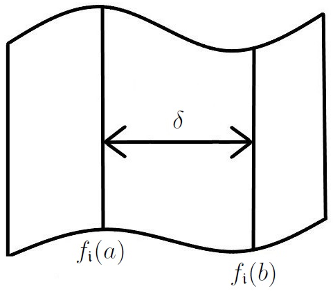
Figure 2: $S_{\mathfrak{i}}([0,1]^{2})$ together with two points $f_{\mathfrak{i}}(a)$ and $f_{\mathfrak{i}}(b)$ which together form a vertical strip of width $\delta$.

We have shown that the height of the intersection of $S_{\mathfrak{i}}([0,1]^{2})$ with every vertical strip with base length $\delta$ is at most $k^{\prime}\delta$, where $k^{\prime}$ is independent of $\mathfrak{i}$. Thus at most $k=\lceil k^{\prime}\rceil+1$ squares in any column of the $\delta$-mesh intersect $S_{\mathfrak{i}}([0,1]^{2})$ so using (4.2) $\mathcal{D}^{q}_{\delta}(\mu_{\mathfrak{i}})\asymp\mathcal{D}^{q}_{\delta}(\pi\mu_{\mathfrak{i}})$ where $\pi\mu_{\mathfrak{i}}$ is the projection of $\mu_{\mathfrak{i}}$ onto the $x$-axis. In terms of the projection of pre-images of the intersection of $\delta$-mesh cubes $Q$ with $S_{\mathfrak{i}}([0,1]^{2})$,

$$\mathcal{D}^{q}_{\delta}(\mu_{\mathfrak{i}}) =\sum_{Q\in\mathcal{D}_{\delta}}\mu_{\mathfrak{i}}\left(Q\cap S_{\mathfrak{i}}([0,1]^{2})\right)^{q}$$

$$=p(\mathfrak{i})^{q}\sum_{Q\in\mathcal{D}_{\delta}}\mu\left(S_{\mathfrak{i}}^{-1}\left(Q\cap S_{\mathfrak{i}}([0,1]^{2})\right)\right)^{q}$$

$$\asymp p(\mathfrak{i})^{q}\sum_{Q\in\mathcal{D}_{\delta}}\pi\mu\left(\pi S_{\mathfrak{i}}^{-1}\left(Q\cap S_{\mathfrak{i}}([0,1]^{2})\right)\right)^{q}.$$ (4.8)

If $Q$ is a $\delta$-mesh cube that intersects $S_{\mathfrak{i}}([0,1]^{2})$ other than one overlapping its left or right edge, then $\pi S_{\mathfrak{i}}^{-1}\left(Q\cap S_{\mathfrak{i}}([0,1]^{2})\right)$ is an interval in $\mathbb{R}$ of length $\delta$. Writing $\hat{a},\hat{b}$ for the endpoints of $\pi S_{\mathfrak{i}}^{-1}\left(Q\cap S_{\mathfrak{i}}([0,1]^{2})\right)$ then using the mean value theorem and (3.14),

$$|\hat{a}-\hat{b}|\ =\ \frac{|f_{\mathfrak{i}}(\hat{a})-f_{\mathfrak{i}}(\hat{b})|}{|f_{\mathfrak{i},x}(\hat{c})|}\ =\ \frac{\delta}{|f_{\mathfrak{i},x}(\hat{c})|}\ \asymp\ \frac{\delta}{\alpha_{1}(D_{\textbf{a}}S_{\mathfrak{i}})},$$

where $\hat{c}\in[0,1]$.

If $Q$ is one of the two cubes at the left or right end of $S_{\mathfrak{i}}([0,1]^{2})$ then we simply “glue” $\pi S_{\mathfrak{i}}^{-1}\left(Q\cap S_{\mathfrak{i}}([0,1]^{2})\right)$ to the adjacent interval (which will be on the right or left respectively). This will create a new interval which also has length comparable to $\delta/\alpha_{1}(D_{\textbf{a}}S_{\mathfrak{i}})$.

Every projection of a pre-image $\pi S_{\mathfrak{i}}^{-1}\left(Q\cap S_{\mathfrak{i}}([0,1]^{2})\right)$ can be covered by an interval of length $\widehat{A}\delta/\alpha_{1}(D_{\textbf{a}}S_{\mathfrak{i}})$ and contains an interval of length $\widehat{B}\delta/\alpha_{1}(D_{\textbf{a}}S_{\mathfrak{i}})$, for some constants $\widehat{A}\geq\widehat{B}>0$. Recall the definitions (4.3) of $\widehat{A}_{\mathfrak{i},\delta}$ and $\widehat{B}_{\mathfrak{i},\delta}$ and write $\mathcal{J}_{\delta}$ for the $\delta$-mesh on $\mathbb{R}$ centred at the origin. From (4.8), noting that each $J\in\mathcal{J}_{\widehat{A}_{\mathfrak{i},\delta}}$ can intersect $\pi S_{\mathfrak{i}}^{-1}\left(Q\cap S_{\mathfrak{i}}([0,1]^{2})\right)$ for at most $k\big{\lceil}\widehat{A}/\widehat{B}+1\big{\rceil}$ many $Q\in\mathcal{D}_{\delta}$, and using (4.2),

$$\mathcal{D}^{q}_{\delta}(\mu_{\mathfrak{i}}) \asymp p(\mathfrak{i})^{q}\sum_{Q\in\mathcal{D}_{\delta}}\pi\mu\left(\pi S_{\mathfrak{i}}^{-1}\left(Q\cap S_{\mathfrak{i}}([0,1]^{2})\right)\right)^{q}$$

$$\lesssim p(\mathfrak{i})^{q}\sum_{J\in\mathcal{J}_{\widehat{A}_{\mathfrak{i},\delta}}}\pi\mu(J)^{q}$$

$$=\sum_{J\in\mathcal{J}_{\widehat{A}_{\mathfrak{i},\delta}}}(p(\mathfrak{i})\pi\mu(J))^{q}$$

$$=\mathcal{D}^{q}_{\widehat{A}_{\mathfrak{i},\delta}}(p(\mathfrak{i})\pi\mu).$$

Similarly, each $\pi S_{\mathfrak{i}}^{-1}\left(Q\cap S_{\mathfrak{i}}([0,1]^{2})\right)$ intersects at most $\big{\lceil}\widehat{A}/\widehat{B}+1\big{\rceil}$ intervals $J\in\mathcal{J}_{\widehat{B}_{\mathfrak{i},\delta}}$, and each interval $J\in\mathcal{J}_{\widehat{B}_{\mathfrak{i},\delta}}$ intersects $\pi S_{\mathfrak{i}}^{-1}\left(Q\cap S_{\mathfrak{i}}([0,1]^{2})\right)$ for at most $2k$ sets $Q\in\mathcal{D}_{\delta}$, so

$$\mathcal{D}^{q}_{\delta}(\mu_{\mathfrak{i}}) \asymp p(\mathfrak{i})^{q}\sum_{Q\in\mathcal{D}_{\delta}}\pi\mu\left(\pi S_{\mathfrak{i}}^{-1}\left(Q\cap S_{\mathfrak{i}}([0,1]^{2})\right)\right)^{q}$$

$$\gtrsim p(\mathfrak{i})^{q}\sum_{J\in\mathcal{J}_{\widehat{B}_{\mathfrak{i},\delta}}}\pi\mu(J)^{q}$$

$$=\sum_{J\in\mathcal{J}_{\widehat{B}_{\mathfrak{i},\delta}}}(p(\mathfrak{i})\pi\mu(J))^{q}$$

$$=\mathcal{D}^{q}_{\widehat{B}_{\mathfrak{i},\delta}}(p(\mathfrak{i})\pi\mu),$$

giving the result. ∎

Notice that a simple consequence of the Definition 1.3 of the $L^{q}$-spectrum is that for all $\varepsilon>0,q\geq 0,p>0$ and $0<\delta\leq 1$

$$p^{q}\delta^{-\beta(q)+\varepsilon/2}\lesssim_{\varepsilon,q}\mathcal{D}^{q}_{\delta}(p\pi\mu)\lesssim_{\varepsilon,q}p^{q}\delta^{-\beta(q)-\varepsilon/2}$$ (4.9)

We now turn to proving our main result, Theorem 3.8.

Proof of Theorem 3.8.

The first two parts of this proof follow Fraser’s proof of [12, Theorem 2.6] but we reproduce it here due to its centrality to our result.

Part (1). Let $q\in[0,1]$ and let $\delta\in(0,1]$ and $\textbf{a}\in[0,1]^{2}$. It is sufficient to show that $\overline{\tau}_{\mu}(q)\leq\gamma(q)$. As $q\in[0,1]$,

$$\mathcal{D}^{q}_{\delta}(\mu)=\sum_{Q\in\mathcal{D}_{\delta}}\mu(Q)^{q}=\sum_{Q\in\mathcal{D}_{\delta}}\Big{(}\sum_{\mathfrak{i}\in\mathcal{I}_{\delta}}\mu_{\mathfrak{i}}(Q)\Big{)}^{q}\leq\sum_{Q\in\mathcal{D}_{\delta}}\sum_{\mathfrak{i}\in\mathcal{I}_{\delta}}\mu_{\mathfrak{i}}(Q)^{q} =\sum_{\mathfrak{i}\in\mathcal{I}_{\delta}}\sum_{Q\in\mathcal{D}_{\delta}}\mu_{\mathfrak{i}}(Q)^{q}$$

$$=\sum_{\mathfrak{i}\in\mathcal{I}_{\delta}}\mathcal{D}^{q}_{\delta}(\mu_{\mathfrak{i}}).$$

Thus for all $\varepsilon>0$,

$$\delta^{\gamma(q)+\varepsilon}\mathcal{D}_{\delta}^{q}(\mu)\ \leq\ \delta^{\gamma(q)+\varepsilon}\sum_{\mathfrak{i}\in\mathcal{I}_{\delta}}\mathcal{D}^{q}_{\delta}(\mu_{\mathfrak{i}})$$

$$\lesssim\ \delta^{\gamma(q)+\varepsilon}\sum_{\mathfrak{i}\in\mathcal{I}_{\delta}}\mathcal{D}^{q}_{\widehat{A}_{\mathfrak{i},\delta}}(p(\mathfrak{i})\pi_{\mathfrak{i}}\mu)$$ by (4.4)

$$\lesssim_{\varepsilon,q}\ \delta^{\gamma(q)+\varepsilon}\sum_{\mathfrak{i}\in\mathcal{I}_{\delta}}p(\mathfrak{i})^{q}\left(\frac{\widehat{A}\delta}{\alpha_{1}(D_{\textbf{a}}S_{\mathfrak{i}})}\right)^{-\beta(q)-\varepsilon/2}$$ by (4.9)

$$\lesssim_{\varepsilon,q}\ \sum_{\mathfrak{i}\in\mathcal{I}_{\delta}}p(\mathfrak{i})^{q}\alpha_{1}(D_{\textbf{a}}S_{\mathfrak{i}})^{\beta(q)+\varepsilon/2}\alpha_{2}(D_{\textbf{a}}S_{\mathfrak{i}})^{\gamma(q)+\varepsilon-\beta(q)-\varepsilon/2}$$ by (4.1)

$$=\ \ \ \sum_{\mathfrak{i}\in\mathcal{I}_{\delta}}\psi^{\gamma(q)+\varepsilon,q}_{\textbf{a}}(\mathfrak{i})$$ by (3.18)

$$\lesssim_{\varepsilon,q}1.$$ by Lemma 4.1

So $\overline{\tau}_{\mu}(q)\leq\gamma(q)+\varepsilon$ by (1.2), giving (1) on letting $\varepsilon\to 0$ .

Part (2). We suppose $q\geq 1$ and as before let $\delta\in(0,1]$ and $\textbf{a}\in[0,1]^{2}$. It is sufficient to show that $\underline{\tau}_{\mu}(q)\geq\gamma(q)$. As $q\geq 1$,

$$\mathcal{D}^{q}_{\delta}(\mu)=\sum_{Q\in\mathcal{D}_{\delta}}\mu(Q)^{q}=\sum_{Q\in\mathcal{D}_{\delta}}\Big{(}\sum_{\mathfrak{i}\in\mathcal{I}_{\delta}}\mu_{\mathfrak{i}}(Q)\Big{)}^{q}\geq\sum_{Q\in\mathcal{D}_{\delta}}\sum_{\mathfrak{i}\in\mathcal{I}_{\delta}}\mu_{\mathfrak{i}}(Q)^{q} =\sum_{\mathfrak{i}\in\mathcal{I}_{\delta}}\sum_{Q\in\mathcal{D}_{\delta}}\mu_{\mathfrak{i}}(Q)^{q}$$

$$=\sum_{\mathfrak{i}\in\mathcal{I}_{\delta}}\mathcal{D}^{q}_{\delta}(\mu_{\mathfrak{i}}).$$

Thus for all $\varepsilon>0$,

$$\delta^{\gamma(q)-\varepsilon}\mathcal{D}_{\delta}^{q}(\mu)\ \geq\ \delta^{\gamma(q)-\varepsilon}\sum_{\mathfrak{i}\in\mathcal{I}_{\delta}}\mathcal{D}^{q}_{\delta}(\mu_{\mathfrak{i}})$$

$$\gtrsim\ \delta^{\gamma(q)-\varepsilon}\sum_{\mathfrak{i}\in\mathcal{I}_{\delta}}\mathcal{D}^{q}_{\widehat{B}_{\mathfrak{i},\delta}}(p(\mathfrak{i})\pi_{\mathfrak{i}}\mu)$$ by (4.4)

$$\gtrsim_{\varepsilon,q}\ \delta^{\gamma(q)-\varepsilon}\sum_{\mathfrak{i}\in\mathcal{I}_{\delta}}p(\mathfrak{i})^{q}\left(\frac{\widehat{B}\delta}{\alpha_{1}(D_{\textbf{a}}S_{\mathfrak{i}})}\right)^{-\beta(q)+\varepsilon/2}$$ by (4.9)

$$\gtrsim_{\varepsilon,q}\ \sum_{\mathfrak{i}\in\mathcal{I}_{\delta}}p(\mathfrak{i})^{q}\alpha_{1}(D_{\textbf{a}}S_{\mathfrak{i}})^{\beta(q)-\varepsilon/2}\alpha_{2}(D_{\textbf{a}}S_{\mathfrak{i}})^{\gamma(q)-\varepsilon-\beta(q)+\varepsilon/2}$$ by (4.1)

$$=\ \ \ \sum_{\mathfrak{i}\in\mathcal{I}_{\delta}}\psi^{\gamma(q)-\varepsilon,q}_{\textbf{a}}(\mathfrak{i})$$ by (3.18)

$$\gtrsim_{\varepsilon,q}1.$$ by Lemma 4.1

So $\underline{\tau}_{\mu}(q)\geq\gamma(q)-\varepsilon$ giving (2) on letting $\varepsilon\to 0$.

Part (3) We now assume $\mu$ satisfies the ROSC. Due to Parts (1) and (2) we only need to provide an upper bound when $q>1$ and a lower bound when $q<1$.

We begin by considering the case when $q>1$. For (1) we obtained an upper bound when $q\in[0,1]$, but the only place in the proof where we used the assumption $q\leq 1$ was

$$\mathcal{D}^{q}_{\delta}(\mu)\leq\sum_{\mathfrak{i}\in\mathcal{I}_{\delta}}\mathcal{D}^{q}_{\delta}(\mu_{\mathfrak{i}}).$$

Thus for $q>1$ we shall use the ROSC to show that

$$\mathcal{D}^{q}_{\delta}(\mu)\lesssim\sum_{\mathfrak{i}\in\mathcal{I}_{\delta}}\mathcal{D}^{q}_{\delta}(\mu_{\mathfrak{i}}).$$

It follows from Hölder’s inequality that for $Q\in\mathcal{D}_{\delta}$

$$\Big{(}\sum_{\mathfrak{i}\in\mathcal{I}_{\delta}}\mu_{\mathfrak{i}}(Q)\Big{)}^{q}\leq\ k^{q-1}\sum_{\mathfrak{i}\in\mathcal{I}_{\delta}}\mu_{\mathfrak{i}}(Q)^{q}$$

where

$$k:=|\{\mathfrak{i}\in\mathcal{I}_{\delta}:\mu_{\mathfrak{i}}(Q)>0\}|.$$ (4.10)

To complete the proof we need to bound $k$ uniformly for all $\delta$ and $Q\in\mathcal{D}_{\delta}$. Fix $\delta\in(0,1]$ and $Q\in\mathcal{D}_{\delta}$ such that $\mu(Q)>0$. Let $R$ denote the open unit square $(0,1)^{2}$. For convenience if $A>0$ then we write $AQ$ to denote the cube with the same centre as $Q$ but with sidelength $A\delta$.

Let $\mathfrak{i}\in\mathcal{I}_{\delta}$ be such that $S_{\mathfrak{i}}(R)\cap Q$ is non-empty (such an $\mathfrak{i}$ must exist as by assumption $\mu(Q)>0$). Let $\textbf{a}\in S_{\mathfrak{i}}(R)\cap Q$ and consider the vertical “slice” of $S_{\mathfrak{i}}(R)$ that contains a. By (4.1) and Lemma 3.4, $g_{\mathfrak{i},y}(\textbf{a})\asymp\alpha_{2}(D_{\textbf{a}}S_{\mathfrak{i}})\asymp\delta$. Together with the mean value theorem this implies that the height of this vertical slice is comparable to $\delta$, say it is bounded above by $M\delta$ for some $M>1$ which is independent of $\delta$.

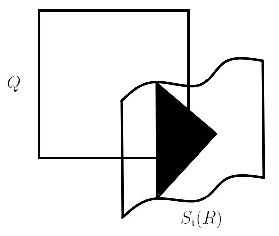
Figure 3: $S_{\mathfrak{i}}(R)$ and $Q$, together with the triangle $\Delta_{\mathfrak{i}}$ contained in $S_{\mathfrak{i}}(R)$.

Lemma 4.2 implies that if we draw a line of slope $L$ (where we can assume $L>1$) from the base of the vertical slice in both directions and a line of slope $-L$ from the top of the vertical slice in both directions then of the two isosceles triangles formed by these lines and the vertical slice at least one must lie within $S_{\mathfrak{i}}(R)$. As the length of the vertical slice is comparable to $\delta$ the area of this triangle is comparable to $\delta^{2}$. We write $\Delta_{\mathfrak{i}}$ for the triangle which is contained in $S_{\mathfrak{i}}(R)$.

Each triangle $\Delta_{\mathfrak{i}}$ (associated with $\mathfrak{i}\in\mathcal{I}_{\delta}$ such that $S_{\mathfrak{i}}(R)\cap Q\neq\emptyset$) is contained in the square which has the same centre as $Q$ and sidelength $3M\delta$, i.e. the square $3MQ$. Let $\mathcal{L}$ denote two-dimensional Lebesgue measure. As the area of each $\Delta_{\mathfrak{i}}$ is comparable to $\delta$ and the ROSC guarantees that the interiors of the $\Delta_{\mathfrak{i}}$ are pairwise disjoint, it follows from (4.10) that

$$k\delta^{2}\lesssim\sum_{\begin{subarray}{c}\mathfrak{i}\in\mathcal{I}_{\delta}:\\ S_{\mathfrak{i}}(R)\cap Q\neq\emptyset\end{subarray}}\mathcal{L}(\Delta_{\mathfrak{i}})\leq(3M\delta)^{2}=9M^{2}\delta^{2}.$$

Hence $k\lesssim 1$ completing the proof of the upper bound for $q>1$.

When $0\leq q<1$ a similar approach to the $q>1$ case above establishes that

$$\mathcal{D}^{q}_{\delta}(\mu)\gtrsim\sum_{\mathfrak{i}\in\mathcal{I}_{\delta}}\mathcal{D}^{q}_{\delta}(\mu_{\mathfrak{i}}).$$

We omit the proof which is very similar. ∎

Acknowledgements

KJF and JMF were supported by an EPSRC Standard Grant (EP/R015104/1). JMF was also supported by a Leverhulme Trust Research Project Grant (RPG-2019-034). LDL was supported by an EPSRC Doctoral Training Grant.

Kenneth J. Falconer, School of Mathematics & Statistics, University of St Andrews, St Andrews, KY16 9SS, UK E-mail address: kjf@st-andrews.ac.uk

Jonathan M. Fraser, School of Mathematics & Statistics, University of St Andrews, St Andrews, KY16 9SS, UK E-mail address: jmf32@st-andrews.ac.uk

Lawrence D. Lee, School of Mathematics & Statistics, University of St Andrews, St Andrews, KY16 9SS, UK E-mail address: ldl@st-andrews.ac.uk

References

[1] B. Bárány. Subadditive Pressure for IFS with Triangular Maps. Bull. Pol. Acad. Sci. Math., 57, (2009), 263-278.
[2]
J. Barral and D.-J. Feng.
Multifractal formalism for almost all self-affine measures.
Comm. Math. Phys., 318, (2013), 473-504.
[3] L. Barreira. Thermodynamic Formalism and Applications to Dimension Theory. Birkhäuser, (2011).
[4] Y. Cao, Y. Pesin and Y. Zhao. Dimension Estimates for Non-Conformal Repellers and Continuity of Sub-additive Topological Pressure. Geom. Func. Anal., 29, (2019), 1325-1368.
[5] K. J. Falconer. Bounded distortion and dimension for non-conformal repellers. Math. Proc. Cambridge Philos. Soc. 115, (1994), 315-334.
[6] K. J. Falconer. Techniques in Fractal Geometry. Wiley (1997).
[7]
K. J. Falconer. Generalised dimensions of measures on self-affine sets. Nonlinearity, 12, (1999), 877-891.
[8]
K. J. Falconer. Generalised dimensions of measures on almost self-affine sets. Nonlinearity, 23, (2010), 1047-1069.
[9] K. J. Falconer. Fractal Geometry: Mathematical Foundations and Applications (3rd Ed). Wiley (2014).
[10] K. J. Falconer and J. Miao. Dimensions of self-affine fractals and multifractals generated by upper-triangular matrices. Fractals, 15, (2007), 289-299.
[11] D.-J. Feng and Y. Wang. A class of self-affine sets and self-affine measures. J. Fourier Anal. App., 11, (2005), 107-124.
[12] J. M. Fraser. On the -spectrum of planar self-affine measures. Trans. Amer. Math. Soc., 368, (2016), 5579-5620.
[13] H. Hu. Dimensions of invariant sets of expanding maps. Comm. Math. Phys., 176, (1996), 307-320.
[14] J. E. Hutchinson. Fractals and self-similarity. Indiana Univ. Math. J., 30, (1981), 713-747.
[15] I. Kolossváry and K. Simon. Triangular Gatzouras-Lalley-type planar carpets with overlaps. Nonlinearity, 32, (2019), 3294-3341.
[16] A. Manning and K. Simon. Subadditive pressure for triangular maps. Nonlinearity, 20, (2007), 133-149.
[17]
S.-M. Ngai. A dimension result arising from the -spectrum of a measure.
Proc. Amer. Math. Soc., 125, (1997), 2943-2951.
[18] L. Olsen. A multifractal formalism. Adv. Math., 116, (1995), 82-196.
[19] Y. Peres and B. Solomyak. Existence of -dimensions and entropy dimension for self-conformal measures. Indiana Univ. Math. J., 49, (2000), 1603-1621.