Entropy-Augmented Entropy-Regularized Reinforcement Learning and a Continuous Path
from Policy Gradient to Q-Learning

Donghoon Lee
donghoon.paul.lee@gmail.com
Abstract

Entropy augmented to reward is known to soften the greedy argmax policy to softmax policy. Entropy augmentation is reformulated and leads to a motivation to introduce an additional entropy term to the objective function in the form of KL-divergence to regularize optimization process. It results in a policy which monotonically improves while interpolating from the current policy to the softmax greedy policy. This policy is used to build a continuously parameterized algorithm which optimize policy and Q-function simultaneously and whose extreme limits correspond to policy gradient and Q-learning, respectively. Experiments show that there can be a performance gain using an intermediate algorithm.

Both Q-learning[15] and policy gradient(PG)[13] update policy towards greedy one whether the policy is explicit or not. However, since a greedy deterministic policy is not reachable in a continuous action space or even in a discrete action space under certain policy parameterization, it may benefit to soften the update target. Q-learning suffers from abrupt changes of implicit deterministic policy while continuously updating Q-function. Furthermore, it is required to soften the policy during training for the balance between exploration and exploitation. There have been efforts to incorporate entropy to regularize Q-learning and PG or to expedite exploration [17, 3, 11]. In this work, we optimize entropy-augmented objective function greedily and obtain softmax policy as is well-known in maximum-entropy based frameworks. However, we further regularize the objective function by adding KL-divergence with the current policy itself, which results in a continuously parameterized policy, called advanced policy, expanding two-dimensional surface in policy space.

Recently, connections between Q-learning and PG have been elucidated. [9] showed that soft Q-function update can be decomposed into policy gradient and value function update while [8] proposed PCL algorithm which is reduced to PG or Q-learning under certain conditions. We modify actor-critic PG using the advanced policy. Then, both actor and critic actively participate in optimization process unlike Q-learning or PG. Also, we find that the algorithm interpolates continuously between PG and Q-learning as does the advanced policy between the current policy and the greedy policy.

1 Preliminaries

Consider a Markov decision process(MDP) with a state space, $\mathbb{S}$, an action space, $\mathbb{A}$, and average reward r​(s,a)π‘Ÿπ‘ π‘Žr(s,a). π​(a|s)πœ‹conditionalπ‘Žπ‘ \pi(a|s) and Ps​asβ€²subscriptsuperscript𝑃superscriptπ‘ β€²π‘ π‘ŽP^{s^{\prime}}_{sa} refer to policy and transition probability, respectively. The discount factor, $\gamma$, is in the range (0, 1). We assume tabular cases with finite state and action spaces for simplicity, but non-tabular parametric expression will be derived as needed. Extension to continuous action space is straightforward by replacing sums with integrals and interpreting $\pi$ and Ps​asβ€²subscriptsuperscript𝑃superscriptπ‘ β€²π‘ π‘ŽP^{s^{\prime}}_{sa} as probability densities. State-to-state and state-action-to-state-action transition probabilities are defined as products of π​(a|s)πœ‹conditionalπ‘Žπ‘ \pi(a|s) and Ps​asβ€²subscriptsuperscript𝑃superscriptπ‘ β€²π‘ π‘ŽP^{s^{\prime}}_{sa}.

PΒ―ssβ€²=βˆ‘aπ​(a|s)​Ps​asβ€²andPΒ―s​as′​aβ€²=Ps​as′​π​(sβ€²|aβ€²)formulae-sequencesubscriptsuperscript¯𝑃superscript𝑠′𝑠subscriptπ‘Žπœ‹conditionalπ‘Žπ‘ subscriptsuperscript𝑃superscriptπ‘ β€²π‘ π‘Žandsubscriptsuperscript¯𝑃superscript𝑠′superscriptπ‘Žβ€²π‘ π‘Žsubscriptsuperscript𝑃superscriptπ‘ β€²π‘ π‘Žπœ‹conditionalsuperscript𝑠′superscriptπ‘Žβ€²\underaccent{\bar}{P}^{s^{\prime}}_{s}=\sum_{a}\pi(a|s)P^{s^{\prime}}_{sa}\quad\mathrm{and}\quad\bar{P}^{s^{\prime}a^{\prime}}_{sa}=P^{s^{\prime}}_{sa}\pi(s^{\prime}|a^{\prime}) (1)

Then, discounted cumulative transition functions can be expressed in terms of $\underaccent{\bar}{P}^{s^{\prime}}_{s}$ and PΒ―s​as′​aβ€²subscriptsuperscript¯𝑃superscript𝑠′superscriptπ‘Žβ€²π‘ π‘Ž\bar{P}^{s^{\prime}a^{\prime}}_{sa}.

$\displaystyle\underaccent{\bar}{G}^{s^{\prime}}_{s}=\mathbb{I}^{s^{\prime}}_{s}+\gamma\underaccent{\bar}{P}^{s^{\prime}}_{s}+\gamma^{2}\sum_{s_{1}}\underaccent{\bar}{P}^{s_{1}}_{s}\underaccent{\bar}{P}^{s^{\prime}}_{s_{1}}+\cdots$ (2)
GΒ―s​as′​aβ€²=𝕀s​as′​aβ€²+γ​PΒ―s​as′​aβ€²+Ξ³2β€‹βˆ‘s1,a1PΒ―s​as1​a1​PΒ―s1​a1s′​aβ€²+β‹―subscriptsuperscript¯𝐺superscript𝑠′superscriptπ‘Žβ€²π‘ π‘Žsubscriptsuperscript𝕀superscript𝑠′superscriptπ‘Žβ€²π‘ π‘Žπ›Ύsubscriptsuperscript¯𝑃superscript𝑠′superscriptπ‘Žβ€²π‘ π‘Žsuperscript𝛾2subscriptsubscript𝑠1subscriptπ‘Ž1subscriptsuperscript¯𝑃subscript𝑠1subscriptπ‘Ž1π‘ π‘Žsubscriptsuperscript¯𝑃superscript𝑠′superscriptπ‘Žβ€²subscript𝑠1subscriptπ‘Ž1β‹―\displaystyle\bar{G}^{s^{\prime}a^{\prime}}_{sa}=\mathbb{I}^{s^{\prime}a^{\prime}}_{sa}+\gamma\bar{P}^{s^{\prime}a^{\prime}}_{sa}+\gamma^{2}\sum_{s_{1},a_{1}}\bar{P}^{s_{1}a_{1}}_{sa}\bar{P}^{s^{\prime}a^{\prime}}_{s_{1}a_{1}}+\cdots (3)

These sums converge due to $\gamma$. The state- and action-value functions can be written as

Vπ​(s)=βˆ‘sβ€²,aβ€²GΒ―ss′​π​(aβ€²|sβ€²)​r​(sβ€²,aβ€²)andQπ​(s,a)=βˆ‘sβ€²,aβ€²GΒ―s​as′​a′​r​(sβ€²,aβ€²)formulae-sequencesuperscriptπ‘‰πœ‹π‘ subscriptsuperscript𝑠′superscriptπ‘Žβ€²superscriptsubscript¯𝐺𝑠superscriptπ‘ β€²πœ‹conditionalsuperscriptπ‘Žβ€²superscriptπ‘ β€²π‘Ÿsuperscript𝑠′superscriptπ‘Žβ€²andsuperscriptπ‘„πœ‹π‘ π‘Žsubscriptsuperscript𝑠′superscriptπ‘Žβ€²subscriptsuperscript¯𝐺superscript𝑠′superscriptπ‘Žβ€²π‘ π‘Žπ‘Ÿsuperscript𝑠′superscriptπ‘Žβ€²V^{\pi}(s)=\sum_{s^{\prime},a^{\prime}}\underaccent{\bar}{G}_{s}^{s^{\prime}}\pi(a^{\prime}|s^{\prime})r(s^{\prime},a^{\prime})\quad\mathrm{and}\quad Q^{\pi}(s,a)=\sum_{s^{\prime},a^{\prime}}\bar{G}^{s^{\prime}a^{\prime}}_{sa}r(s^{\prime},a^{\prime}) (4)

The objective function is the average of value function over the distribution of initial states.

Ξ·Ο€=βˆ‘s0ρo​(s0)​V​(s0)=βˆ‘sρπ​(s)β€‹βˆ‘aπ​(a|s)​r​(s,a)subscriptπœ‚πœ‹subscriptsubscript𝑠0subscriptπœŒπ‘œsubscript𝑠0𝑉subscript𝑠0subscript𝑠subscriptπœŒπœ‹π‘ subscriptπ‘Žπœ‹conditionalπ‘Žπ‘ π‘Ÿπ‘ π‘Ž\eta_{\pi}=\sum_{s_{0}}\rho_{o}(s_{0})V(s_{0})=\sum_{s}\rho_{\pi}(s)\sum_{a}\pi(a|s)r(s,a) (5)

where $\rho_{\pi}$ is the discounted cumulative state distribution.

ρπ​(s)=βˆ‘s0ρo​(s0)​Gs0ssubscriptπœŒπœ‹π‘ subscriptsubscript𝑠0subscriptπœŒπ‘œsubscript𝑠0subscriptsuperscript𝐺𝑠subscript𝑠0\displaystyle\rho_{\pi}(s)=\sum_{s_{0}}\rho_{o}(s_{0})G^{s}_{s_{0}} (6)

Entropy can be added to encourage exploration. Subscript $\alpha$ denotes inclusion of entropy with temperature $\alpha$. It is common practice to omit the first entropy term in the definition of $Q_{\alpha}$.

$\displaystyle Q^{\pi}_{\alpha}(s,a)=\mathbb{E}_{(s_{t},a_{t})\sim\pi}\left(\left.r(s_{0},a_{0})+\sum_{t=1}\gamma^{t}[r(s_{t},a_{t})+\alpha H(\pi(\cdot|s_{t}))]\right|s_{0}=s,a_{0}=a\right)$ (7)
$\displaystyle V^{\pi}_{\alpha}(s)=\mathbb{E}_{(s_{t},a_{t})\sim\pi}\left(\left.\sum_{t=0}\gamma^{t}[r(s_{t},a_{t})+\alpha H(\pi(\cdot|s_{t}))]\right|s_{0}=s\right)$ (8)

and their corresponding Bellman operators are, in decoupled forms,

Tπ​Qα​(s,a)=r​(s,a)+Ξ³β€‹βˆ‘sβ€²,aβ€²Ps​as′​π​(aβ€²|sβ€²)​[Qα​(sβ€²,aβ€²)βˆ’Ξ±β€‹log⁑π​(aβ€²|sβ€²)]superscriptπ‘‡πœ‹subscriptπ‘„π›Όπ‘ π‘Žπ‘Ÿπ‘ π‘Žπ›Ύsubscriptsuperscript𝑠′superscriptπ‘Žβ€²subscriptsuperscript𝑃superscriptπ‘ β€²π‘ π‘Žπœ‹conditionalsuperscriptπ‘Žβ€²superscript𝑠′delimited-[]subscript𝑄𝛼superscript𝑠′superscriptπ‘Žβ€²π›Όπœ‹conditionalsuperscriptπ‘Žβ€²superscript𝑠′\displaystyle T^{\pi}Q_{\alpha}(s,a)=r(s,a)+\gamma\sum_{s^{\prime},a^{\prime}}P^{s^{\prime}}_{sa}\pi(a^{\prime}|s^{\prime})[Q_{\alpha}(s^{\prime},a^{\prime})-\alpha\log\pi(a^{\prime}|s^{\prime})] (9)
Tπ​Vα​(s)=βˆ‘aπ​(a|s)​[r​(s,a)βˆ’Ξ±β€‹log⁑π​(a|s)]+Ξ³β€‹βˆ‘a,s′π​(a|s)​Ps​as′​Vα​(sβ€²)superscriptπ‘‡πœ‹subscript𝑉𝛼𝑠subscriptπ‘Žπœ‹conditionalπ‘Žπ‘ delimited-[]π‘Ÿπ‘ π‘Žπ›Όπœ‹conditionalπ‘Žπ‘ π›Ύsubscriptπ‘Žsuperscriptπ‘ β€²πœ‹conditionalπ‘Žπ‘ subscriptsuperscript𝑃superscriptπ‘ β€²π‘ π‘Žsubscript𝑉𝛼superscript𝑠′\displaystyle T^{\pi}V_{\alpha}(s)=\sum_{a}\pi(a|s)[r(s,a)-\alpha\log\pi(a|s)]+\gamma\sum_{a,s^{\prime}}\pi(a|s)P^{s^{\prime}}_{sa}V_{\alpha}(s^{\prime}) (10)

It is straightforward to show that $\pi^{*}=\frac{1}{Z}\exp\frac{Q_{\alpha}}{\alpha}$ maximizes βˆ‘aπ​(a|s)​[Qα​(s,a)βˆ’Ξ±β€‹log⁑π​(a|s)]subscriptπ‘Žπœ‹conditionalπ‘Žπ‘ delimited-[]subscriptπ‘„π›Όπ‘ π‘Žπ›Όπœ‹conditionalπ‘Žπ‘ \sum_{a}\pi(a|s)[Q_{\alpha}(s,a)-\alpha\log\pi(a|s)] in Eq.(9) and the softmax policy improves over the current policy. Therefore, we can reach the optimal policy and value functions by repeatedly applying soft policy iteration [4]. Omitting the first entropy term is intuitively justified since we do not need to consider the entropy of the current state or action to decide which action to take. Furthermore, it seems crucial in order to apply soft policy improvement theorem that the first reward term on RHS of Eq.(9) does not include entropy.

2 Entropy-Augmented Reinforcement Learning

2.1 Entropy Augmentation to Reward

We start from the definition of entropy-augmented reward and follow the standard formulation.

r~π​(a|s)=r​(s,a)βˆ’Ξ±β€‹log⁑π​(a|s)subscript~π‘Ÿπœ‹conditionalπ‘Žπ‘ π‘Ÿπ‘ π‘Žπ›Όπœ‹conditionalπ‘Žπ‘ \tilde{r}_{\pi}(a|s)=r(s,a)-\alpha\log\pi(a|s) (11)

Both $-\alpha\log\pi$ and $-\alpha\sum\pi\log\pi$ will be referred to as entropy, and $\alpha$ and/or $\pi$ in $Q^{\pi}_{\alpha}$, $V^{\pi}_{\alpha}$ and $\tilde{r}_{\pi}$ will be omitted whenever it is not confusing. Then, the entropy-augmented objective function to maximize is

Ξ·~Ο€=βˆ‘sρπ​(s)β€‹βˆ‘aπ​(a|s)​r~​(s,a)subscript~πœ‚πœ‹subscript𝑠subscriptπœŒπœ‹π‘ subscriptπ‘Žπœ‹conditionalπ‘Žπ‘ ~π‘Ÿπ‘ π‘Ž\tilde{\eta}_{\pi}=\sum_{s}\rho_{\pi}(s)\sum_{a}\pi(a|s)\tilde{r}(s,a) (12)

State- and action-value functions are re-defined canonically as the sum of entropy-augmented rewards. Then, they differ from soft value functions by only the first entropy term.

Q~​(s,a)=βˆ’Ξ±β€‹log⁑π​(a|s)+Q​(s,a)~π‘„π‘ π‘Žπ›Όπœ‹conditionalπ‘Žπ‘ π‘„π‘ π‘Ž\displaystyle\tilde{Q}(s,a)=-\alpha\log\pi(a|s)+Q(s,a) (13)
V~​(s)=βˆ‘aπ​(a|s)​Q~​(s,a)=V​(s)~𝑉𝑠subscriptπ‘Žπœ‹conditionalπ‘Žπ‘ ~π‘„π‘ π‘Žπ‘‰π‘ \displaystyle\tilde{V}(s)=\sum_{a}\pi(a|s)\tilde{Q}(s,a)=V(s) (14)
A~​(s,a)=Q~​(s,a)βˆ’V~​(s)=βˆ’Ξ±β€‹log⁑π​(a|s)+A​(s,a)~π΄π‘ π‘Ž~π‘„π‘ π‘Ž~π‘‰π‘ π›Όπœ‹conditionalπ‘Žπ‘ π΄π‘ π‘Ž\displaystyle\tilde{A}(s,a)=\tilde{Q}(s,a)-\tilde{V}(s)=-\alpha\log\pi(a|s)+A(s,a) (15)

and their corresponding Bellman operators are defined in the standard forms.

T~π​Q~​(s,a)=r~​(s,a)+Ξ³β€‹βˆ‘sβ€²,aβ€²Ps​as′​π​(aβ€²|sβ€²)​Q~​(sβ€²,aβ€²)superscript~π‘‡πœ‹~π‘„π‘ π‘Ž~π‘Ÿπ‘ π‘Žπ›Ύsubscriptsuperscript𝑠′superscriptπ‘Žβ€²superscriptsubscriptπ‘ƒπ‘ π‘Žsuperscriptπ‘ β€²πœ‹conditionalsuperscriptπ‘Žβ€²superscript𝑠′~𝑄superscript𝑠′superscriptπ‘Žβ€²\displaystyle\tilde{T}^{\pi}\tilde{Q}(s,a)=\tilde{r}(s,a)+\gamma\sum_{s^{\prime},a^{\prime}}P_{sa}^{s^{\prime}}\pi(a^{\prime}|s^{\prime})\tilde{Q}(s^{\prime},a^{\prime}) (16)
T~π​V~​(s)=βˆ‘aπ​(a|s)​r~​(s,a)+Ξ³β€‹βˆ‘sβ€²,aπ​(a|s)​Ps​as′​V~​(sβ€²)superscript~π‘‡πœ‹~𝑉𝑠subscriptπ‘Žπœ‹conditionalπ‘Žπ‘ ~π‘Ÿπ‘ π‘Žπ›Ύsubscriptsuperscriptπ‘ β€²π‘Žπœ‹conditionalπ‘Žπ‘ superscriptsubscriptπ‘ƒπ‘ π‘Žsuperscript𝑠′~𝑉superscript𝑠′\displaystyle\tilde{T}^{\pi}\tilde{V}(s)=\sum_{a}\pi(a|s)\tilde{r}(s,a)+\gamma\sum_{s^{\prime},a}\pi(a|s)P_{sa}^{s^{\prime}}\tilde{V}(s^{\prime}) (17)

These are all parallel to the standard formulation of reinforcement learning except that $r$ is replaced by $\tilde{r}$ and depends on $\pi$. While $Q$ and $V$ are greedily optimized simultaneously by $\pi^{*}=\frac{1}{Z}\exp\frac{Q}{\alpha}$, $\tilde{Q}$ is not due to the entropy term in $\tilde{r}$. Note that maximizing $Q$ does not necessarily mean that $\sum_{a}\pi Q$ is maximized. However, this is not a problem since VΞ±β‰ βˆ‘aπ​QΞ±subscript𝑉𝛼subscriptπ‘Žπœ‹subscript𝑄𝛼V_{\alpha}\neq\sum_{a}\pi Q_{\alpha} for non-zero $\alpha$ and what we have to optimize is $V_{\alpha}$ rather than $\sum_{a}\pi Q_{\alpha}$.

2.2 In-state Greedy Optimization

Now, we try to optimize the objective function $\tilde{\eta}$ instead of $V$. Policy gradient of $\tilde{\eta}$ will be considered later. Instead, we try greedy optimization of $\tilde{\eta}$ as with policy improvement. Next lemma is the extension of Eq.(2) in [10] to entropy-augmented cases. Proofs for all theorems and lemmas will be presented in the Appendix.

Lemma 1 (Difference of Objective Functions).

Let $\tilde{\eta}_{\pi^{\prime}}$ and $\tilde{\eta}_{\pi}$ be the expected sums of entropy-augmented rewards for $\pi^{\prime}$ and $\pi$, respectively. Then, their difference is given by

Ξ·~Ο€β€²βˆ’Ξ·~Ο€=βˆ‘sρπ′​(s)β€‹βˆ‘aπ′​(a|s)​(A~π​(s,a)βˆ’Ξ±β€‹log⁑π′​(a|s)π​(a|s))subscript~πœ‚superscriptπœ‹β€²subscript~πœ‚πœ‹subscript𝑠subscript𝜌superscriptπœ‹β€²π‘ subscriptπ‘Žsuperscriptπœ‹β€²conditionalπ‘Žπ‘ superscript~π΄πœ‹π‘ π‘Žπ›Όsuperscriptπœ‹β€²conditionalπ‘Žπ‘ πœ‹conditionalπ‘Žπ‘ \tilde{\eta}_{\pi^{\prime}}-\tilde{\eta}_{\pi}=\sum_{s}\rho_{\pi^{\prime}}(s)\sum_{a}\pi^{\prime}(a|s)\left(\tilde{A}^{\pi}(s,a)-\alpha\log\frac{\pi^{\prime}(a|s)}{\pi(a|s)}\right) (18)

Since ρπ′​(s)β‰₯0subscript𝜌superscriptπœ‹β€²π‘ 0\rho_{\pi^{\prime}}(s)\geq 0, it is guaranteed that $\tilde{\eta}_{\pi^{\prime}}\geq\tilde{\eta}_{\pi}$ if βˆ‘aπ′​(a|s)​(A~π​(s,a)βˆ’Ξ±β€‹log⁑π′​(a|s)π​(a|s))β‰₯0subscriptπ‘Žsuperscriptπœ‹β€²conditionalπ‘Žπ‘ superscript~π΄πœ‹π‘ π‘Žπ›Όsuperscriptπœ‹β€²conditionalπ‘Žπ‘ πœ‹conditionalπ‘Žπ‘ 0\sum_{a}\pi^{\prime}(a|s)\left(\tilde{A}^{\pi}(s,a)-\alpha\log\frac{\pi^{\prime}(a|s)}{\pi(a|s)}\right)\geq 0 for all $s$ with constraint βˆ‘aπ​(a|s)=1subscriptπ‘Žπœ‹conditionalπ‘Žπ‘ 1\sum_{a}\pi(a|s)=1. This leads to "in-state" greedy optimization, which makes the most of the knowledge of current value functions without transition probabilities available.

Theorem 1 (In-State Greedy Optimization).

For any policy $\pi$, βˆ‘aπ′​(a|s)​(A~​(s,a)βˆ’Ξ±β€‹log⁑π′​(a|s)π​(a|s))subscriptπ‘Žsuperscriptπœ‹β€²conditionalπ‘Žπ‘ ~π΄π‘ π‘Žπ›Όsuperscriptπœ‹β€²conditionalπ‘Žπ‘ πœ‹conditionalπ‘Žπ‘ \sum_{a}\pi^{\prime}(a|s)\left(\tilde{A}(s,a)-\alpha\log\frac{\pi^{\prime}(a|s)}{\pi(a|s)}\right) is maximized by $\pi^{\prime}=\frac{1}{Z}\pi\exp\frac{\tilde{A}}{\alpha}$ and $\tilde{\eta}_{\pi^{\prime}}\geq\tilde{\eta}_{\pi}$ holds, where $Z$ is a normalizing factor and the equality holds if and only if $\tilde{A}$ vanishes.

The optimizer policy can be expressed in terms of either $\tilde{A}$ or $\tilde{Q}$.

$$\pi^{\prime}=\frac{1}{Z_{A}}\pi\exp\frac{\tilde{A}}{\alpha}=\frac{1}{Z_{Q}}\pi\exp\frac{\tilde{Q}}{\alpha}$$ (19)

The form of $\pi^{\prime}$ seems different from the softmax greedy policy but the first entropy term of $\tilde{Q}=-\alpha\log\pi+Q$ cancels out the original policy, $\pi$, and $\pi^{\prime}$ can be rewritten as

$$\pi^{\prime}=\frac{1}{Z_{A}}\exp\frac{A}{\alpha}=\frac{1}{Z_{Q}}\exp{\frac{Q}{\alpha}}$$ (20)

For an optimal policy, $\pi^{*}=\frac{1}{Z_{A}}\pi^{*}\exp{\frac{\tilde{A}^{*}}{\alpha}}=\frac{1}{Z_{Q}}\pi^{*}\exp\frac{\tilde{Q}^{*}}{\alpha}$ holds. It is clear that optimality of $\pi^{*}$ is equivalent to $\tilde{Q}^{*}$ and $\tilde{A}^{*}$ being independent of actions. Then, the following holds.

Q~βˆ—β€‹(s,a)superscript~π‘„π‘ π‘Ž\displaystyle\tilde{Q}^{*}(s,a) $\displaystyle=\tilde{V}^{*}(s)$ (21)
A~βˆ—β€‹(s,a)superscript~π΄π‘ π‘Ž\displaystyle\tilde{A}^{*}(s,a) $\displaystyle=0$ (22)

The partition function, $Z_{Q}=\sum_{a}\pi\exp{\frac{\tilde{Q}}{\alpha}}$, is bounded due to the convexity of exponential function[16, 3].

$$Z_{Q}\geq\exp\frac{\tilde{V}}{\alpha}\quad\mathrm{or}\quad\alpha\log Z_{Q}\geq\tilde{V}$$ (23)

Equality holds for an optimal policy. From the definition of $Z_{A}$, it is clear that

$\displaystyle Z_{A}=Z_{Q}\exp\left(-\frac{\tilde{V}}{\alpha}\right)\quad\mathrm{and}\quad Z_{A}\geq 1$ (24)
Remark.

While $\tilde{Q}_{\alpha}$ and $\tilde{A}_{\alpha}$ are action-independent when optimal, $Q$ and $A$ are not in ordinary RL. This is due to the first entropy term, $-\alpha\log\pi$. In this sense, it is not $\tilde{Q}_{\alpha}$ but $Q_{\alpha}$ which is reduced to $Q$ as $\alpha\rightarrow 0$. We could have avoided this problem by defining $\tilde{r}=r-\alpha\sum_{a}\pi\log\pi$ instead of $\tilde{r}=r-\alpha\log\pi$ without modifying $\tilde{\eta}_{\pi}$. Then, it would have held that $\pi^{*}=\frac{1}{Z}\exp{\frac{\tilde{Q}}{\alpha}}$ rather than $\pi^{*}=\frac{1}{Z}\pi\exp{\frac{\tilde{Q}}{\alpha}}$. This is a matter of choice but the latter form is preferred since it shows how the optimizing process modifies the current policy to softmax greedy policy.
Eq.(22) implies that $\tilde{A}$ is not the measure of how good an action is but that of how adequate the probability of an action is. Whenever A~​(s,a)>0~π΄π‘ π‘Ž0\tilde{A}(s,a)>0, we have to lower it towards zero by increasing π​(a|s)πœ‹conditionalπ‘Žπ‘ \pi(a|s) and vice versa. In fact, $\tilde{A}$ can be considered as soft consistency error in [8].

2.3 Soft Policy Gradient

The implication of $\tilde{A}$ as critic is more clarified by policy gradient of entropy-augmented RL. It is convenient to know the change of $\rho_{\pi}$ under small variation of $\pi$.

Lemma 2.

For an infinitesimal variation of policy, $\delta\pi$, the corresponding variation of ρπ​(s)​π​(a|s)subscriptπœŒπœ‹π‘ πœ‹conditionalπ‘Žπ‘ \rho_{\pi}(s)\pi(a|s) to first order of $\delta\pi$ is given by

δ​(ρπ​(s)​π​(a|s))=βˆ‘sβ€²,a′ρπ​(sβ€²)​δ​π​(aβ€²|sβ€²)​GΒ―sβ€²,aβ€²s,a𝛿subscriptπœŒπœ‹π‘ πœ‹conditionalπ‘Žπ‘ subscriptsuperscript𝑠′superscriptπ‘Žβ€²subscriptπœŒπœ‹superscriptπ‘ β€²π›Ώπœ‹conditionalsuperscriptπ‘Žβ€²superscript𝑠′subscriptsuperscriptΒ―πΊπ‘ π‘Žsuperscript𝑠′superscriptπ‘Žβ€²\delta(\rho_{\pi}(s)\pi(a|s))=\sum_{s^{\prime},a^{\prime}}\rho_{\pi}(s^{\prime})\delta\pi(a^{\prime}|s^{\prime})\bar{G}^{s,a}_{s^{\prime},a^{\prime}} (25)

Formula for soft PG is same as that of standard PG except that $A$ has to be replaced by $\tilde{A}$.

Theorem 2 (Soft Policy Gradient).

Let $\tilde{\eta}_{\pi}$ be the expected sum of entropy-augmented rewards and $\pi$ be parameterized by $\theta$, then the following holds.

βˆ‡ΞΈΞ·~Ο€=βˆ‘sρπ​(s)β€‹βˆ‘aπ​(a|s)β€‹βˆ‡ΞΈlog⁑π​(a|s)​A~​(s,a)subscriptβˆ‡πœƒsubscript~πœ‚πœ‹subscript𝑠subscriptπœŒπœ‹π‘ subscriptπ‘Žπœ‹conditionalπ‘Žπ‘ subscriptβˆ‡πœƒπœ‹conditionalπ‘Žπ‘ ~π΄π‘ π‘Ž\nabla_{\theta}\tilde{\eta}_{\pi}=\sum_{s}\rho_{\pi}(s)\sum_{a}\pi(a|s)\nabla_{\theta}\log\pi(a|s)\tilde{A}(s,a) (26)

Soft policy gradient of the same objective function was derived in [11] and it is equivalent to Eq.(26) up to a baseline function. Also, the gradient estimator of [9] with KL-divergence regularization can be shown equivalent to Eq.(26) if the reference policy, $\bar{\pi}$, in [9] is set to a uniform probability distribution.

Remark.

Eq.(26) also shows that $\tilde{A}$ is the critic which tells how to adjust the probability of an action. The fixed point of PG is simply where $\tilde{A}$ vanishes and Eq.(26) can be considered as policy improvement step towards $\frac{1}{Z}\exp\frac{A}{\alpha}$. Note that, in standard PG without $-\alpha\log\pi$, the policy is updated indefinitely towards a greedy policy, which can be harmful especially if $\pi$ is parameterized.

3 Regularization of Greedy Policy to Advanced Policy

3.1 Regularization by KL-divergence

With entropy-augmentation to rewards, the policy does not collapse to a deterministic one. However, the original policy is completely forgotten because the first entropy term in $\tilde{Q}$ cancels it out. This motivates us to apply an additional regularization to the optimization process. Especially, we do not want to drive the policy too far from the current policy. For this purpose we add a KL-divergence term to the objective function and repeat the in-state greedy optimization.

Ξ·~Ο€β€²βˆ’Ξ·~Ο€βˆ’Ξ²β€‹βˆ‘sρπ′​DK​L​(Ο€β€²|Ο€)=βˆ‘sρπ′​(s)β€‹βˆ‘aπ′​(a|s)​(A~α​(s,a)βˆ’(Ξ±+Ξ²)​log⁑π′​(a|s)π​(a|s))subscript~πœ‚superscriptπœ‹β€²subscript~πœ‚πœ‹π›½subscript𝑠subscript𝜌superscriptπœ‹β€²subscript𝐷𝐾𝐿conditionalsuperscriptπœ‹β€²πœ‹subscript𝑠subscript𝜌superscriptπœ‹β€²π‘ subscriptπ‘Žsuperscriptπœ‹β€²conditionalπ‘Žπ‘ subscript~π΄π›Όπ‘ π‘Žπ›Όπ›½superscriptπœ‹β€²conditionalπ‘Žπ‘ πœ‹conditionalπ‘Žπ‘ \tilde{\eta}_{\pi^{\prime}}-\tilde{\eta}_{\pi}-\beta\sum_{s}\rho_{\pi^{\prime}}D_{KL}(\pi^{\prime}|\pi)=\sum_{s}\rho_{\pi^{\prime}}(s)\sum_{a}\pi^{\prime}(a|s)\left(\tilde{A}_{\alpha}(s,a)-(\alpha+\beta)\log\frac{\pi^{\prime}(a|s)}{\pi(a|s)}\right) (27)

Then, the original policy is modified by a softmax multiplicative factor.

$$\pi^{\prime}=\frac{1}{Z}\pi\exp\frac{\tilde{A}_{\alpha}}{(\alpha+\beta)}$$ (28)

It seems that we simply added more regularization. However, the original policy is only partially cancelled as expected.

$$\pi^{\prime}=\frac{1}{Z}\pi^{\frac{\beta}{\alpha+\beta}}\exp\frac{A_{\alpha}}{(\alpha+\beta)}=\frac{1}{Z}\pi^{\frac{\beta}{\alpha+\beta}}(e^{\frac{A_{\alpha}}{\alpha}})^{\frac{\alpha}{(\alpha+\beta)}}$$ (29)

The last expression implies that the regularized optimizer policy is along the linear interpolation of the original policy and the softmax greedy policy in terms of logit values. Let us call this "advanced policy" and it is more convenient to replace $\frac{1}{\alpha+\beta}$ with $\epsilon$.

$\displaystyle\pi^{\prime}_{\epsilon}=\frac{1}{Z_{A}}\pi\exp{\epsilon\tilde{A}_{\alpha}}=\frac{1}{Z_{A}}\pi^{(1-\epsilon\alpha)}\exp\epsilon A_{\alpha}$ (30)

$\epsilon=0$ and $\epsilon=\frac{1}{\alpha}$ correspond to the current policy and the softmax greedy policy, respectively. It should be emphasized that we added entropy in two ways but they are not parallel. $\alpha$ controls how soft the greedily optimized policy is whereas $\beta$ controls how far the optimization process goes from the current policy. Now, we have a continuous path, linear in logit space, from the current policy to the greedily optimized policy, which has nice properties. Also, in the proof of Theorem 3, it will be shown that KL-divergence regularization can be converted to KL-divergence constraint.

Theorem 3 (Monotonic Improvement of Advanced Policy).

For any policy $\pi$ and its advanced policy $\pi^{\prime}_{\epsilon}=\frac{1}{Z_{A}}\pi\exp\epsilon\tilde{A}$, the objective function, Ξ·~πϡ′=βˆ‘sρπϡ′​(s)β€‹βˆ‘aπϡ′​(a|s)​r~′​(s,a)subscript~πœ‚subscriptsuperscriptπœ‹β€²italic-Ο΅subscript𝑠subscript𝜌subscriptsuperscriptπœ‹β€²italic-ϡ𝑠subscriptπ‘Žsubscriptsuperscriptπœ‹β€²italic-Ο΅conditionalπ‘Žπ‘ superscript~π‘Ÿβ€²π‘ π‘Ž\tilde{\eta}_{\pi^{\prime}_{\epsilon}}=\sum_{s}\rho_{\pi^{\prime}_{\epsilon}}(s)\sum_{a}\pi^{\prime}_{\epsilon}(a|s)\tilde{r}^{\prime}(s,a), is an increasing function of $\epsilon$. It is a constant function if $\pi$ is optimal.

Corollary 1 (Simultaneous Optimality of Advanced Policy).

For any policy $\pi$, its advanced policy, $\pi^{\prime}_{\epsilon}=\frac{1}{Z_{A}}\pi\exp\epsilon\tilde{A}$, is either optimal or non-optimal for all $\epsilon$. Equivalently, advanced policy is optimal if and only if $\tilde{A}$ vanishes.

Corollary 2 (Advanced Policy Improvement Theorem).

For any policy $\pi$ and its advanced policy $\pi^{\prime}_{\epsilon}=\frac{1}{Z_{A}}\pi\exp\epsilon\tilde{A}$, the following holds for any (s,a)π‘ π‘Ž(s,a) and for any $\epsilon$ such that $0<\epsilon\leq\frac{1}{\alpha}$.

Vπϡ′​(s)β‰₯Vπ​(s)andQπϡ′​(s,a)β‰₯Qπ​(s,a)formulae-sequencesuperscript𝑉subscriptsuperscriptπœ‹β€²italic-ϡ𝑠superscriptπ‘‰πœ‹π‘ andsuperscript𝑄subscriptsuperscriptπœ‹β€²italic-Ο΅π‘ π‘Žsuperscriptπ‘„πœ‹π‘ π‘ŽV^{\pi^{\prime}_{\epsilon}}(s)\geq V^{\pi}(s)\quad\mathrm{and}\quad Q^{\pi^{\prime}_{\epsilon}}(s,a)\geq Q^{\pi}(s,a) (31)

Equalities hold if $\pi$ is optimal.

Note that Corollary 2 holds for soft $Q$ but not for $\tilde{Q}$. Please see also [12] and [4].

3.2 Infinitely Regularized Limit and Policy Gradient

To investigate the behavior of the advanced policy near the current policy, we expand partition functions in Taylor series at $\epsilon=0$.

$\displaystyle Z_{Q}=1+\epsilon\tilde{V}+O(\epsilon^{2})$ (32)
$\displaystyle Z_{A}=1+O(\epsilon^{2})$ (33)

Now, we can find the direction of advanced policy from the current policy.

Theorem 4 (Derivative of Advanced Policy).

For a given policy, $\pi$, and its advantage function, $\tilde{A}$, the derivative of $\pi_{\epsilon}^{\prime}=\frac{1}{Z}\pi\exp\epsilon\tilde{A}$ with respect to $\epsilon$ at $\epsilon=0$ is given by

$$\left.\frac{d\pi_{\epsilon}^{\prime}}{d\epsilon}\right|_{\epsilon=0}=\pi\tilde{A}$$ (34)

Informally, the infinitesimal variation of policy under small change of $\epsilon$ can be written as $\delta\pi=\delta\epsilon\pi\tilde{A}$ or $\delta\log\pi=\delta\epsilon\tilde{A}$. If $\pi$ is parameterized by $\theta$, $\delta\log\pi$ can be written in terms of $\delta\theta$.

$$\nabla_{\theta}\log\pi\cdot\delta\theta=\delta\epsilon\tilde{A}$$ (35)

This is usually an over-determined problem since the number of state-action pairs is larger than that of the elements of $\theta$, and can be solved using weighted least square method. $\nabla_{\theta}\log\pi$ is treated as matrix whose row is indexed by (s,a)π‘ π‘Ž(s,a).

βˆ‘s,aρπ​π​(βˆ‡ΞΈlog⁑π)Tβ€‹βˆ‡ΞΈlog⁑π⋅δ​θ=Ξ΄β€‹Ο΅β€‹βˆ‘s,aρπ​π​(βˆ‡ΞΈlog⁑π)T​A~subscriptπ‘ π‘ŽsubscriptπœŒπœ‹πœ‹superscriptsubscriptβˆ‡πœƒπœ‹π‘‡subscriptβˆ‡πœƒβ‹…πœ‹π›Ώπœƒπ›Ώitalic-Ο΅subscriptπ‘ π‘ŽsubscriptπœŒπœ‹πœ‹superscriptsubscriptβˆ‡πœƒπœ‹π‘‡~𝐴\sum_{s,a}\rho_{\pi}\pi(\nabla_{\theta}\log\pi)^{T}\nabla_{\theta}\log\pi\cdot\delta\theta=\delta\epsilon\sum_{s,a}\rho_{\pi}\pi(\nabla_{\theta}\log\pi)^{T}\tilde{A} (36)

The coefficient of LHS is Fisher Information Matrix(FIM) and the above equation can be solved by applying the inverse of FIM. Note that this indicates, whether soft or not, the direction of greedy policy improvement at the original policy is along the natural gradient.

Corollary 3 (Natural Policy Gradient).

For a policy parameterized by $\theta$, the derivative of $\theta$ with respect to $\epsilon$ along its advanced policy, $\pi^{\prime}_{\epsilon}=\frac{1}{Z}\pi\exp\epsilon\tilde{A}$, at $\epsilon=0$ is given by natural policy gradient.

d​θd​ϡ|Ο΅=0=(βˆ‘s,aρπ​π​(βˆ‡ΞΈlog⁑π)Tβ€‹βˆ‡ΞΈlog⁑π)βˆ’1β‹…βˆ‘s,aρπ​π​(βˆ‡ΞΈlog⁑π)T​A~evaluated-atπ‘‘πœƒπ‘‘italic-Ο΅italic-Ο΅0β‹…superscriptsubscriptπ‘ π‘ŽsubscriptπœŒπœ‹πœ‹superscriptsubscriptβˆ‡πœƒπœ‹π‘‡subscriptβˆ‡πœƒπœ‹1subscriptπ‘ π‘ŽsubscriptπœŒπœ‹πœ‹superscriptsubscriptβˆ‡πœƒπœ‹π‘‡~𝐴\left.\frac{d\theta}{d\epsilon}\right|_{\epsilon=0}=\left(\sum_{s,a}\rho_{\pi}\pi(\nabla_{\theta}\log\pi)^{T}\nabla_{\theta}\log\pi\right)^{-1}\cdot\sum_{s,a}\rho_{\pi}\pi(\nabla_{\theta}\log\pi)^{T}\tilde{A} (37)
Remark.

[10] obtained natural policy gradient by optimizing the local approximator of $\eta$ with KL-divergence constraint. We extended this to entropy-augmented case. [6] showed that, if the policy is parameterized as exponential of linear combination of function approximators, the natural gradient direction leads to the argmax greedy policy. He also showed that, for arbitrarily parameterized policies, the local direction of natural gradient is towards the greedy policy of the local linear compatible approximator for Q. Since we have already showed that advanced policy is the linear interpolation of the current policy and the softmax greedy policy in logit space, both can be considered as special cases of the above result. The advanced policy explicitly shows a path emanating from the current policy in the direction of natural policy gradient and resulting in the (softmax) greedy policy.

Surrogate Objective Functions

Instead of following the gradient of performance objective as in standard policy gradient, we can set a nearby target policy superior to the current policy and try to decrease a distance measure from the target. Advanced policy, $\pi^{\prime}=\frac{1}{Z}\pi\exp{\epsilon\tilde{A}}$, is a natural choice of the target and negative KL-divergence can be used as surrogate objective function to maximize.

Jϡ​(Ο€,Ο€o)=βˆ’βˆ‘s,aρπo​DK​L​(Ο€|1ZAo​πo​exp⁑ϡ​A~o)subscript𝐽italic-Ο΅πœ‹subscriptπœ‹π‘œsubscriptπ‘ π‘Žsubscript𝜌subscriptπœ‹π‘œsubscript𝐷𝐾𝐿conditionalπœ‹1subscript𝑍subscriptπ΄π‘œsubscriptπœ‹π‘œitalic-Ο΅subscript~π΄π‘œJ_{\epsilon}(\pi,\pi_{o})=-\sum_{s,a}\rho_{\pi_{o}}D_{KL}\left(\pi\left|\frac{1}{Z_{A_{o}}}\pi_{o}\exp{\epsilon\tilde{A}_{o}}\right.\right) (38)

, where $\pi_{o}$ is the current policy. Derivation of policy gradient of $J_{\epsilon}$ is not complicated. Surprisingly, we reproduce the standard policy gradient for any $\epsilon$.

βˆ‡ΞΈJΟ΅=Ο΅β€‹βˆ‘s,aΟΟ€β€‹Ο€β€‹βˆ‡ΞΈlog⁑π​A~subscriptβˆ‡πœƒsubscript𝐽italic-Ο΅italic-Ο΅subscriptπ‘ π‘ŽsubscriptπœŒπœ‹πœ‹subscriptβˆ‡πœƒπœ‹~𝐴\nabla_{\theta}J_{\epsilon}=\epsilon\sum_{s,a}\rho_{\pi}\pi\nabla_{\theta}\log\pi\tilde{A} (39)

For $\epsilon=\frac{1}{\alpha}$, this corresponds to Soft Actor Critic update rule[4]. However, this is not the unique form of policy gradient since KL-divergence is not the only possible measure of distance. Another simple choice of surrogate objective function is

J=βˆ’12β€‹βˆ‘s,aρπo​(Ο€βˆ’Ο€oβ€²)2J12subscriptπ‘ π‘Žsubscript𝜌subscriptπœ‹π‘œsuperscriptπœ‹superscriptsubscriptπœ‹π‘œβ€²2\textit{J}=-\frac{1}{2}\sum_{s,a}\rho_{\pi_{o}}(\pi-\pi_{o}^{\prime})^{2} (40)

The policy gradient of this can be found using Taylor expansion of $\pi^{\prime}$ in terms of $\epsilon$.

βˆ‡ΞΈJ=Ο΅β€‹βˆ‘s,aΟΟ€β€‹Ο€β€‹βˆ‡ΞΈΟ€β€‹A~+O​(Ο΅2)subscriptβˆ‡πœƒJitalic-Ο΅subscriptπ‘ π‘ŽsubscriptπœŒπœ‹πœ‹subscriptβˆ‡πœƒπœ‹~𝐴𝑂superscriptitalic-Ο΅2\nabla_{\theta}\textit{J}=\epsilon\sum_{s,a}\rho_{\pi}\pi\nabla_{\theta}\pi\tilde{A}+O(\epsilon^{2}) (41)

Eq.(39) and Eq.(41) are reminiscent of cross-entropy loss and L2 loss, respectively. Please see Appendix for derivations. Note that, in spite of the difference of forms, they all share the same fixed point. The gradients vanish when $\tilde{A}=0$ or $\alpha\log\pi=A$.

4 A Path from Policy Gradient to Q-Learning

4.1 Advanced Actor Critic

A simple application of advanced policy is to run PG of $\pi$ and use its advanced policy for test with some $\epsilon$. However, our goal is to find a continuously parameterized algorithm which encompasses PG and Q-learning to elucidate the relation between them, which is not straightforward since the latter optimize Q-function directly without any explicit policy while, in PG, policy is optimized and the critic plays only a passive role of assessing the policy. To bridge the gap, we can make both actor and critic participate in optimization. Corollary 1 and Theorem 3 imply that we can optimize the advanced policy instead of the current policy and Corollary 2 implies that advanced policy can be used for Q-function update target. We start from a policy and a Q-function parameterized by $\theta$ and $\phi$, respectively, and apply actor-critic PG algorithm on the hybrid policy, $\pi^{\prime}=\frac{1}{Z}\pi_{\theta}^{(1-\epsilon\alpha)}\exp{\epsilon Q_{\phi}}$.

$\displaystyle\Delta\theta$ βˆβˆ‘sρπ′​(s)β€‹βˆ‘aπ′​(a|s)β€‹βˆ‡ΞΈlog⁑π′​(a|s)​(Q​(s,a)βˆ’Ξ±β€‹log⁑π′)proportional-toabsentsubscript𝑠subscript𝜌superscriptπœ‹β€²π‘ subscriptπ‘Žsuperscriptπœ‹β€²conditionalπ‘Žπ‘ subscriptβˆ‡πœƒsuperscriptπœ‹β€²conditionalπ‘Žπ‘ π‘„π‘ π‘Žπ›Όsuperscriptπœ‹β€²\displaystyle\propto\sum_{s}\rho_{\pi^{\prime}}(s)\sum_{a}\pi^{\prime}(a|s)\nabla_{\theta}\log\pi^{\prime}(a|s)(Q(s,a)-\alpha\log\pi^{\prime}) (42)
$\displaystyle\Delta\phi$ βˆπ”Ό(s,a)∼(ρ′,Ο€β€²)​(Q^​(s,a)βˆ’Q​(s,a))β€‹βˆ‡Ο•Q​(s,a)proportional-toabsentsubscript𝔼similar-toπ‘ π‘ŽsuperscriptπœŒβ€²superscriptπœ‹β€²^π‘„π‘ π‘Žπ‘„π‘ π‘Žsubscriptβˆ‡italic-Ο•π‘„π‘ π‘Ž\displaystyle\propto\mathbb{E}_{(s,a)\sim(\rho^{\prime},\pi^{\prime})}\left(\hat{Q}(s,a)-Q(s,a)\right)\nabla_{\phi}Q(s,a) (43)
whereQ^​(s,a)=r​(s,a)+γ​𝔼(sβ€²,aβ€²)∼(ρ′,Ο€β€²)​(Qϕ¯​(sβ€²,aβ€²)βˆ’Ξ±β€‹log⁑π′​(aβ€²|sβ€²))where^π‘„π‘ π‘Žπ‘Ÿπ‘ π‘Žπ›Ύsubscript𝔼similar-tosuperscript𝑠′superscriptπ‘Žβ€²superscriptπœŒβ€²superscriptπœ‹β€²subscript𝑄¯italic-Ο•superscript𝑠′superscriptπ‘Žβ€²π›Όsuperscriptπœ‹β€²conditionalsuperscriptπ‘Žβ€²superscript𝑠′\displaystyle\quad\mathrm{where}\quad\hat{Q}(s,a)=r(s,a)+\gamma\mathbb{E}_{(s^{\prime},a^{\prime})\sim(\rho^{\prime},\pi^{\prime})}\left(Q_{\bar{\phi}}(s^{\prime},a^{\prime})-\alpha\log\pi^{\prime}(a^{\prime}|s^{\prime})\right) (44)

Eq.(43) is in accordance with Eq.(9), and $\bar{\phi}$ is the parameter of target network. Seemingly, we are running just an entropy-augmented actor critic PG. The difference is that $Q$ is not passive any more but tries to optimize itself as with Q-learning. Note that $Q$ is being updated towards $Q_{\pi^{\prime}}$, but $Q_{\pi^{\prime}}$ moves further as $Q$ approaches $Q_{\pi^{\prime}}$ since $\pi^{\prime}$ depends on $Q$. Each of the above two equations alone can not reach the optimal policy or Q-function without each other, but the simultaneous fixed point is $(\pi^{*},Q^{*})$. For $\epsilon$ between 0 and $\frac{1}{\alpha}$, both $\pi$ and $Q$ actively participate in the optimization process and $\epsilon$ tells which is more active. When $\epsilon=0$, the above update rules become those of ordinary (soft) actor-critic PG. At the other extreme limit where $\epsilon=\frac{1}{\alpha}$, $\pi^{\prime}$ drops $\pi$ and becomes softmax policy of $Q$. Then, Eq.(43) is reduced to (soft) Q-learning and Eq.(42) vanishes identically. The pseudo code for this algorithm is in Algorithm 1.

Remark.

Implementation of this algorithm in a discrete action space is trivial since we can calculate $\pi^{\prime}$ from the sum of the logits of $\pi$ and $Q$. Actually, we can modify most variants of actor-critic PG algorithm using advanced policy. Rules are simple. Collect samples from the advanced policy. Update the advanced policy using PG and select actions from the advanced policy for target Q-function.
In fact, we can selectively replace only some of $\pi$ in actor-critic PG with $\pi^{\prime}$ without modifying the fixed point. However, the dynamics of optimization process will be different and broad range of experiments need to be performed to investigate the consequences.

Algorithm 1 Advanced Actor Critic (AAC)
Β Β Initialize πθ​(a|s)subscriptπœ‹πœƒconditionalπ‘Žπ‘ \pi_{\theta}(a|s), Qϕ​(s,a)subscript𝑄italic-Ο•π‘ π‘ŽQ_{\phi}(s,a) and target Qϕ¯​(s,a)subscript𝑄¯italic-Ο•π‘ π‘ŽQ_{\bar{\phi}}(s,a).
Β Β Define $\pi^{\prime}=\frac{1}{Z}\pi^{(1-\epsilon\alpha)}\exp{\epsilon Q}$
Β Β Initialize replay memory R.
Β Β Schedule running, learning and update steps
Β Β forΒ each episodeΒ do
Β Β Β Β Β forΒ runningΒ do
Β Β Β Β Β Β Β Β atβˆΌΟ€β€²,st+1∼Pst​atst+1formulae-sequencesimilar-tosubscriptπ‘Žπ‘‘superscriptπœ‹β€²similar-tosubscript𝑠𝑑1subscriptsuperscript𝑃subscript𝑠𝑑1subscript𝑠𝑑subscriptπ‘Žπ‘‘a_{t}\sim\pi^{\prime}\mathrm{,}\quad s_{t+1}\sim P^{s_{t+1}}_{s_{t}a_{t}}
Β Β Β Β Β Β Β Β (st,at,rt,st+1)β†’Rβ†’subscript𝑠𝑑subscriptπ‘Žπ‘‘subscriptπ‘Ÿπ‘‘subscript𝑠𝑑1𝑅(s_{t},a_{t},r_{t},s_{t+1})\rightarrow R
Β Β Β Β Β endΒ for
Β Β Β Β Β forΒ learningΒ do
Β Β Β Β Β Β Β Β Select (s,a,r,sβ€²)π‘ π‘Žπ‘Ÿsuperscript𝑠′(s,a,r,s^{\prime}) samples from R.
        $\theta\leftarrow\theta+\lambda_{\theta}\mathbb{E}[\nabla_{\theta}\log\pi^{\prime}(Q-\alpha\log\pi^{\prime})]$
        ϕ←ϕ+λϕ​𝔼​[(Q^​(s,a)βˆ’Qϕ​(s,a))β€‹βˆ‡Ο•Qϕ​(s,a)]←italic-Ο•italic-Ο•subscriptπœ†italic-ϕ𝔼delimited-[]^π‘„π‘ π‘Žsubscript𝑄italic-Ο•π‘ π‘Žsubscriptβˆ‡italic-Ο•subscript𝑄italic-Ο•π‘ π‘Ž\phi\leftarrow\phi+\lambda_{\phi}\mathbb{E}[(\hat{Q}(s,a)-Q_{\phi}(s,a))\nabla_{\phi}Q_{\phi}(s,a)]
Β Β Β Β Β Β Β Β Β Β Β Β Β Β  where Q^​(s,a)=r​(s,a)+γ​(Qϕ¯​(sβ€²,aβ€²)βˆ’Ξ±β€‹log⁑π′​(sβ€²,aβ€²)),aβ€²βˆΌΟ€β€²β€‹(aβ€²|sβ€²)formulae-sequence^π‘„π‘ π‘Žπ‘Ÿπ‘ π‘Žπ›Ύsubscript𝑄¯italic-Ο•superscript𝑠′superscriptπ‘Žβ€²π›Όsuperscriptπœ‹β€²superscript𝑠′superscriptπ‘Žβ€²similar-tosuperscriptπ‘Žβ€²superscriptπœ‹β€²conditionalsuperscriptπ‘Žβ€²superscript𝑠′\hat{Q}(s,a)=r(s,a)+\gamma(Q_{\bar{\phi}}(s^{\prime},a^{\prime})-\alpha\log\pi^{\prime}(s^{\prime},a^{\prime})),\quad a^{\prime}\sim\pi^{\prime}(a^{\prime}|s^{\prime})
Β Β Β Β Β endΒ for
Β Β Β Β Β forΒ updateΒ do
        $\bar{\phi}\leftarrow\rho\phi+(1-\rho)\bar{\phi}$
Β Β Β Β Β endΒ for
Β Β endΒ for

4.2 Experiments

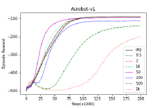
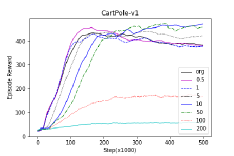
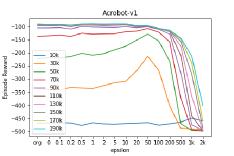
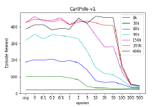
We can extend Advanced Actor Critic(AAC) to variants of actor-critic algorithm by simply replacing $\pi$ with $\pi^{\prime}$. To see the effect of this on environments with discrete action spaces, ACER[14] of advanced policy was tested on a couple of OpenAI Gym environments[1]. Stable-baselines[5] source code was used out of the box with minimal modification to the policy class. Entropy coefficient was set to 0.01 by default for exploration but $Q$ does not include entropy so we assume $\alpha=0$ and valid $\epsilon$ ranges from 0 to $\infty$. See Appendix for source code and settings.
Fig.1 shows episode rewards on Acrobot-v1(left) and CartPole-v1(right) environments for various $\epsilon$ values. We observe that performance deteriorates at large $\epsilon$, where the algorithm becomes more like Q-learning. Graphs on the bottom compare performances as a function of $\epsilon$ at some fixed training steps. Left(Acrobot-v1) graphs show that performance curves rise faster than that of the original algorithm at some intermediate values of $\epsilon$. This effect is less prominent in case of Cartpole-v1(right). Instead, the episode reward rises slowly but remains stable at large training steps. However, it is not certain whether AAC with certain finite $\epsilon$ is superior to PG or it is only an ensemble effect from the combination of $\pi$ and $Q$.

Refer to caption
Refer to caption
Refer to caption
Refer to caption
Figure 1: Top:Training curve of episode rewards for various $\epsilon$. Bottom:Comparison at fixed training steps. Each plot is the average of 100 training results.

Sampling from advanced policy in a continuous action space is complicated. However, it is common to assume a Gaussian policy with its mean and standard deviation parameterized by neural nets. If we further assume that the policy is sharply peaked and $\epsilon$ is small so that $\frac{1}{Z}e^{\epsilon\tilde{Q}}$ is not steep at the peak of $\pi$ and modifies parameters of $\pi$ slightly, $\pi^{\prime}$ can be approximated by a Gaussian distribution with modified mean, $\mu^{\prime}=\mu+\epsilon\sigma^{\prime 2}\frac{dQ}{da}$, and standard deviation, $\sigma^{\prime 2}=\frac{\sigma^{2}}{(1-\epsilon\alpha)}$. SAC[4] and TD3[2] modified with advanced policy were tested but no performance gain was observed. The above modifications are valid only when both $\epsilon$ and $\frac{dQ}{da}$ are small. Due to small $\epsilon$, we cannot investigate the region far from PG. Furthermore, the assumption that $\pi$ is sharply peaked while $Q$ is almost flat is violated as learning proceeds since the peak of the policy and that of Q-function approach each other. Therefore, we need to apply general sampling methods in continuous action spaces such as acceptance-rejection method or MCMC sampling and these will be left for future study.

5 Conclusion

We applied entropy to reinforcement learning along two axes to obtain advanced policy which starts from the current policy in the direction of natural gradient and monotonically improves to (softmax) greedy policy. Then it was used to modify actor-critic PG to build a continuously parameterized algorithm interpolating PG and Q-learning, in which policy and Q-function actively cooperate in the optimization process. Experiments showed a possibility to find an intermediate algorithm performing better than PG or Q-learning though more thorough investigation is needed.

Broader Impact

This work does not present any foreseeable societal consequence.

References

  • [1] Greg Brockman et al. β€œOpenAI Gym” In CoRR abs/1606.01540, 2016 arXiv: http://arxiv.org/abs/1606.01540
  • [2] Scott Fujimoto, Herke Hoof and David Meger β€œAddressing Function Approximation Error in Actor-Critic Methods” In CoRR abs/1802.09477, 2018 arXiv: http://arxiv.org/abs/1802.09477
  • [3] Tuomas Haarnoja, Haoran Tang, Pieter Abbeel and Sergey Levine β€œReinforcement Learning with Deep Energy-Based Policies” In Proceedings of the 34th International Conference on Machine Learning - Volume 70, ICML’17 Sydney, NSW, Australia: JMLR.org, 2017, pp. 1352–1361
  • [4] Tuomas Haarnoja, Aurick Zhou, Pieter Abbeel and Sergey Levine β€œSoft Actor-Critic: Off-Policy Maximum Entropy Deep Reinforcement Learning with a Stochastic Actor” In CoRR abs/1801.01290, 2018 arXiv: http://arxiv.org/abs/1801.01290
  • [5] Ashley Hill et al. β€œStable Baselines” In GitHub repository GitHub, https://github.com/hill-a/stable-baselines, 2018
  • [6] Sham Kakade β€œA Natural Policy Gradient” In Proceedings of the 14th International Conference on Neural Information Processing Systems: Natural and Synthetic, NIPS’01 Vancouver, British Columbia, Canada: MIT Press, 2001, pp. 1531–1538
  • [7] Sham Kakade and John Langford β€œApproximately Optimal Approximate Reinforcement Learning” In Proceedings of the Nineteenth International Conference on Machine Learning, ICML ’02 San Francisco, CA, USA: Morgan Kaufmann Publishers Inc., 2002, pp. 267–274
  • [8] Ofir Nachum, Mohammad Norouzi, Kelvin Xu and Dale Schuurmans β€œBridging the Gap Between Value and Policy Based Reinforcement Learning” In CoRR abs/1702.08892, 2017 arXiv: http://arxiv.org/abs/1702.08892
  • [9] John Schulman, Pieter Abbeel and Xi Chen β€œEquivalence Between Policy Gradients and Soft Q-Learning” In CoRR abs/1704.06440, 2017 arXiv: http://arxiv.org/abs/1704.06440
  • [10] John Schulman et al. β€œTrust Region Policy Optimization” In Proceedings of the 32nd International Conference on Machine Learning 37, Proceedings of Machine Learning Research Lille, France: PMLR, 2015, pp. 1889–1897 URL: http://proceedings.mlr.press/v37/schulman15.html
  • [11] Wenjie Shi, Shiji Song and Cheng Wu β€œSoft Policy Gradient Method for Maximum Entropy Deep Reinforcement Learning” In Proceedings of the Twenty-Eighth International Joint Conference on Artificial Intelligence International Joint Conferences on Artificial Intelligence Organization, 2019 DOI: 10.24963/ijcai.2019/475
  • [12] Richard S. Sutton and Andrew G. Barto β€œReinforcement Learning: An Introduction” The MIT Press, 2018 URL: http://incompleteideas.net/book/the-book-2nd.html
  • [13] Richard S. Sutton, David McAllester, Satinder Singh and Yishay Mansour β€œPolicy Gradient Methods for Reinforcement Learning with Function Approximation” In Proceedings of the 12th International Conference on Neural Information Processing Systems, NIPS’99 Denver, CO: MIT Press, 1999, pp. 1057–1063
  • [14] Ziyu Wang et al. β€œSample Efficient Actor-Critic with Experience Replay” In CoRR abs/1611.01224, 2016 arXiv: http://arxiv.org/abs/1611.01224
  • [15] Christopher Watkins and Peter Dayan β€œTechnical Note: Q-Learning” In Machine Learning 8, 1992, pp. 279–292 DOI: 10.1007/BF00992698
  • [16] Brian D. Ziebart β€œModeling Purposeful Adaptive Behavior with the Principle of Maximum Causal Entropy” USA: Carnegie Mellon University, 2010
  • [17] Brian D. Ziebart, Andrew Maas, J. Bagnell and Anind K. Dey β€œMaximum Entropy Inverse Reinforcement Learning” In Proceedings of the 23rd National Conference on Artificial Intelligence - Volume 3, AAAI’08 Chicago, Illinois: AAAI Press, 2008, pp. 1433–1438

Appendix

Appendix A Proofs

See 1

Proof.

We start from the following identity (see [10] and [7]).

Ξ·Ο€β€²=Ξ·Ο€+βˆ‘sρπ′​(s)β€‹βˆ‘aπ′​(a|s)​Aπ​(s,a)subscriptπœ‚superscriptπœ‹β€²subscriptπœ‚πœ‹subscript𝑠subscript𝜌superscriptπœ‹β€²π‘ subscriptπ‘Žsuperscriptπœ‹β€²conditionalπ‘Žπ‘ superscriptπ΄πœ‹π‘ π‘Ž\eta_{\pi^{\prime}}=\eta_{\pi}+\sum_{s}\rho_{\pi^{\prime}}(s)\sum_{a}\pi^{\prime}(a|s)A^{\pi}(s,a) (45)

This cannot be applied directly to $\tilde{\eta}$ because $\tilde{r}$ depends on $\pi$ while $\tilde{r}^{\prime}$ depends on $\pi^{\prime}$. However, $-\alpha\log\pi^{\prime}$ can be decomposed as $-\alpha\log\pi-\alpha\log\frac{\pi^{\prime}}{\pi}$ so that they have the same reward form.

$\displaystyle\tilde{\eta}_{\pi^{\prime}}-\tilde{\eta}_{\pi}$ =βˆ‘s,aρπ′​(s)​π′​(a|s)​r~′​(s,a)βˆ’βˆ‘s,aρπ​(s)​π​(a|s)​r~​(s,a)absentsubscriptπ‘ π‘Žsubscript𝜌superscriptπœ‹β€²π‘ superscriptπœ‹β€²conditionalπ‘Žπ‘ superscript~π‘Ÿβ€²π‘ π‘Žsubscriptπ‘ π‘ŽsubscriptπœŒπœ‹π‘ πœ‹conditionalπ‘Žπ‘ ~π‘Ÿπ‘ π‘Ž\displaystyle=\sum_{s,a}\rho_{\pi^{\prime}}(s)\pi^{\prime}(a|s)\tilde{r}^{\prime}(s,a)-\sum_{s,a}\rho_{\pi}(s)\pi(a|s)\tilde{r}(s,a)
=βˆ‘s,aρπ′​(s)​π′​(a|s)​(r~​(s,a)βˆ’Ξ±β€‹log⁑π′​(a|s)π​(a|s))βˆ’βˆ‘s,aρπ​(s)​π​(a|s)​r~​(s,a)absentsubscriptπ‘ π‘Žsubscript𝜌superscriptπœ‹β€²π‘ superscriptπœ‹β€²conditionalπ‘Žπ‘ ~π‘Ÿπ‘ π‘Žπ›Όsuperscriptπœ‹β€²conditionalπ‘Žπ‘ πœ‹conditionalπ‘Žπ‘ subscriptπ‘ π‘ŽsubscriptπœŒπœ‹π‘ πœ‹conditionalπ‘Žπ‘ ~π‘Ÿπ‘ π‘Ž\displaystyle=\sum_{s,a}\rho_{\pi^{\prime}}(s)\pi^{\prime}(a|s)\left(\tilde{r}(s,a)-\alpha\log\frac{\pi^{\prime}(a|s)}{\pi(a|s)}\right)-\sum_{s,a}\rho_{\pi}(s)\pi(a|s)\tilde{r}(s,a)
=βˆ‘s,aρπ′​(s)​π′​(a|s)​r~​(s,a)βˆ’βˆ‘s,aρπ​(s)​π​(a|s)​r~​(s,a)βˆ’βˆ‘s,aρπ′​(s)​π′​(a|s)​α​log⁑π′​(a|s)π​(a|s)absentsubscriptπ‘ π‘Žsubscript𝜌superscriptπœ‹β€²π‘ superscriptπœ‹β€²conditionalπ‘Žπ‘ ~π‘Ÿπ‘ π‘Žsubscriptπ‘ π‘ŽsubscriptπœŒπœ‹π‘ πœ‹conditionalπ‘Žπ‘ ~π‘Ÿπ‘ π‘Žsubscriptπ‘ π‘Žsubscript𝜌superscriptπœ‹β€²π‘ superscriptπœ‹β€²conditionalπ‘Žπ‘ π›Όsuperscriptπœ‹β€²conditionalπ‘Žπ‘ πœ‹conditionalπ‘Žπ‘ \displaystyle=\sum_{s,a}\rho_{\pi^{\prime}}(s)\pi^{\prime}(a|s)\tilde{r}(s,a)-\sum_{s,a}\rho_{\pi}(s)\pi(a|s)\tilde{r}(s,a)-\sum_{s,a}\rho_{\pi^{\prime}}(s)\pi^{\prime}(a|s)\alpha\log\frac{\pi^{\prime}(a|s)}{\pi(a|s)}
=βˆ‘s,aρπ′​(s)​π′​(a|s)​(A~π​(s,a)βˆ’Ξ±β€‹log⁑π′​(a|s)π​(a|s))absentsubscriptπ‘ π‘Žsubscript𝜌superscriptπœ‹β€²π‘ superscriptπœ‹β€²conditionalπ‘Žπ‘ superscript~π΄πœ‹π‘ π‘Žπ›Όsuperscriptπœ‹β€²conditionalπ‘Žπ‘ πœ‹conditionalπ‘Žπ‘ \displaystyle=\sum_{s,a}\rho_{\pi^{\prime}}(s)\pi^{\prime}(a|s)\left(\tilde{A}^{\pi}(s,a)-\alpha\log\frac{\pi^{\prime}(a|s)}{\pi(a|s)}\right) (46)

, where we have applied Eq.(45) to obtain the last result from the third line. Eq.(45) can be applied even if $\tilde{r}=r-\alpha\log\pi$ since it is applicable for an arbitrary reward function as long as the reward functions in the first and the second term coincide. Note that the above result does not hold for soft advantage function, $A_{\alpha}$, since it does not contain the first entropy term. ∎

See 1

Proof.

It is straightforward to show that $\frac{1}{Z}\pi\exp\frac{\tilde{A}}{\alpha}$ is the extremum of $\sum_{a}\pi^{\prime}(\tilde{A}-\alpha\log\frac{\pi^{\prime}}{\pi})$ with constraint $\sum_{a}\pi=1$ using Lagrange multiplier.

$\displaystyle 0$ =βˆ‡ΞΈ[βˆ‘aπ′​(a|s)​(A~​(s,a)βˆ’Ξ±β€‹log⁑π′​(a|s)π​(a|s))]βˆ’Ξ²β€‹βˆ‡ΞΈβ€‹βˆ‘aπ′​(a|s)absentsubscriptβˆ‡πœƒsubscriptπ‘Žsuperscriptπœ‹β€²conditionalπ‘Žπ‘ ~π΄π‘ π‘Žπ›Όsuperscriptπœ‹β€²conditionalπ‘Žπ‘ πœ‹conditionalπ‘Žπ‘ π›½subscriptβˆ‡πœƒsubscriptπ‘Žsuperscriptπœ‹β€²conditionalπ‘Žπ‘ \displaystyle=\nabla_{\theta}\left[\sum_{a}\pi^{\prime}(a|s)\left(\tilde{A}(s,a)-\alpha\log\frac{\pi^{\prime}(a|s)}{\pi(a|s)}\right)\right]-\beta\nabla_{\theta}\sum_{a}\pi^{\prime}(a|s)
=βˆ‘a[βˆ‡ΞΈΟ€β€²β€‹(a|s)​(A~​(s,a)βˆ’Ξ±β€‹log⁑π′​(a|s)π​(a|s))βˆ’Ξ±β€‹Ο€β€²β€‹(a|s)β€‹βˆ‡ΞΈΟ€β€²β€‹(a|s)π′​(a|s)βˆ’Ξ²β€‹βˆ‡ΞΈΟ€β€²β€‹(a|s)]absentsubscriptπ‘Ždelimited-[]subscriptβˆ‡πœƒsuperscriptπœ‹β€²conditionalπ‘Žπ‘ ~π΄π‘ π‘Žπ›Όsuperscriptπœ‹β€²conditionalπ‘Žπ‘ πœ‹conditionalπ‘Žπ‘ π›Όsuperscriptπœ‹β€²conditionalπ‘Žπ‘ subscriptβˆ‡πœƒsuperscriptπœ‹β€²conditionalπ‘Žπ‘ superscriptπœ‹β€²conditionalπ‘Žπ‘ π›½subscriptβˆ‡πœƒsuperscriptπœ‹β€²conditionalπ‘Žπ‘ \displaystyle=\sum_{a}\left[\nabla_{\theta}\pi^{\prime}(a|s)\left(\tilde{A}(s,a)-\alpha\log\frac{\pi^{\prime}(a|s)}{\pi(a|s)}\right)-\alpha\pi^{\prime}(a|s)\frac{\nabla_{\theta}\pi^{\prime}(a|s)}{\pi^{\prime}(a|s)}-\beta\nabla_{\theta}\pi^{\prime}(a|s)\right]
=βˆ‘aβˆ‡ΞΈΟ€β€²β€‹(a|s)​(A~​(s,a)βˆ’Ξ±β€‹log⁑π′​(a|s)π​(a|s)βˆ’Ξ²)absentsubscriptπ‘Žsubscriptβˆ‡πœƒsuperscriptπœ‹β€²conditionalπ‘Žπ‘ ~π΄π‘ π‘Žπ›Όsuperscriptπœ‹β€²conditionalπ‘Žπ‘ πœ‹conditionalπ‘Žπ‘ π›½\displaystyle=\sum_{a}\nabla_{\theta}\pi^{\prime}(a|s)\left(\tilde{A}(s,a)-\alpha\log\frac{\pi^{\prime}(a|s)}{\pi(a|s)}-\beta\right) (47)

, where $\beta$ is a Lagrange multiplier and $\pi^{\prime}$ is assumed parameterized by $\theta$. We assume a tabular parameterization, where $\theta$ is indexed by (s,a)π‘ π‘Ž(s,a) so that ΞΈs​a=π′​(a|s)subscriptπœƒπ‘ π‘Žsuperscriptπœ‹β€²conditionalπ‘Žπ‘ \theta_{sa}=\pi^{\prime}(a|s). Then, βˆ‡ΞΈΟ€β€²β€‹(a|s)subscriptβˆ‡πœƒsuperscriptπœ‹β€²conditionalπ‘Žπ‘ \nabla_{\theta}\pi^{\prime}(a|s) is an identity matrix and A~​(s,a)βˆ’Ξ±β€‹log⁑π′​(a|s)π​(a|s)βˆ’Ξ²=0~π΄π‘ π‘Žπ›Όsuperscriptπœ‹β€²conditionalπ‘Žπ‘ πœ‹conditionalπ‘Žπ‘ π›½0\tilde{A}(s,a)-\alpha\log\frac{\pi^{\prime}(a|s)}{\pi(a|s)}-\beta=0 must hold for each (s,a)π‘ π‘Ž(s,a) at the greedily optimized policy, which results in $\pi^{\prime}=\frac{1}{Z}\pi\exp\frac{\tilde{A}}{\alpha}$.
We have to show that $\frac{1}{Z}\pi\exp\frac{\tilde{A}}{\alpha}$ is actually the maximum of $\sum_{a}\pi^{\prime}(\tilde{A}-\alpha\log\frac{\pi^{\prime}}{\pi})$. For this purpose, we write arbitrary policy $\pi^{\prime}$ as $\frac{1}{Z}\psi\pi\exp\frac{\tilde{A}}{\alpha}$ with normalization constraint for $\psi$. Then,

βˆ‘aπ′​(a|s)​(A~​(s,a)βˆ’Ξ±β€‹log⁑π′​(a|s)π​(a|s))subscriptπ‘Žsuperscriptπœ‹β€²conditionalπ‘Žπ‘ ~π΄π‘ π‘Žπ›Όsuperscriptπœ‹β€²conditionalπ‘Žπ‘ πœ‹conditionalπ‘Žπ‘ \displaystyle\sum_{a}\pi^{\prime}(a|s)\left(\tilde{A}(s,a)-\alpha\log\frac{\pi^{\prime}(a|s)}{\pi(a|s)}\right) $\displaystyle=\sum_{a}\pi^{\prime}\left(\alpha\log Z-\alpha\log\psi\right)$
$\displaystyle=\alpha\log Z-\alpha\sum\pi^{\prime}\left[\log\pi^{\prime}-\log\left(\frac{1}{Z}\pi\exp\frac{\tilde{A}}{\alpha}\right)\right]$
$\displaystyle=\alpha\log Z-\alpha D_{KL}\left(\pi^{\prime}\left|\frac{1}{Z}\pi\log\frac{\tilde{A}}{\alpha}\right.\right)$ (48)

$\alpha\log Z$ depends only on $\pi$ but not on $\pi^{\prime}$ and the second term, $D_{KL}$, has minimum value when $\pi^{\prime}=\frac{1}{Z}\pi\log\frac{\tilde{A}}{\alpha}$. Therefore, we conclude that the sum attains its maximum value $\alpha\log Z$ at $\frac{1}{Z}\pi\log\frac{\tilde{A}}{\alpha}$. Furthermore, from the definition of $Z$ and the convexity of exponential function, it can be shown that

$$Z=\sum_{a}\pi\exp\frac{\tilde{A}}{\alpha}\geq\exp\left(\sum_{a}\pi\frac{\tilde{A}}{\alpha}\right)=1$$ (49)

Therefore, the maximum value is non-negative. The equality holds when $\tilde{A}$ is constant, that is, $\tilde{A}$ vanishes.
By Lemma 1, the difference of objective functions is given by

Ξ·~Ο€β€²βˆ’Ξ·~Ο€=βˆ‘sρπ′​(s)β€‹βˆ‘aπ′​(a|s)​(A~​(s,a)βˆ’Ξ±β€‹log⁑π′​(a|s)π​(a|s))subscript~πœ‚superscriptπœ‹β€²subscript~πœ‚πœ‹subscript𝑠subscript𝜌superscriptπœ‹β€²π‘ subscriptπ‘Žsuperscriptπœ‹β€²conditionalπ‘Žπ‘ ~π΄π‘ π‘Žπ›Όsuperscriptπœ‹β€²conditionalπ‘Žπ‘ πœ‹conditionalπ‘Žπ‘ \tilde{\eta}_{\pi^{\prime}}-\tilde{\eta}_{\pi}=\sum_{s}\rho_{\pi^{\prime}}(s)\sum_{a}\pi^{\prime}(a|s)\left(\tilde{A}(s,a)-\alpha\log\frac{\pi^{\prime}(a|s)}{\pi(a|s)}\right) (50)

Since $\rho_{\pi^{\prime}}\geq 0$ for all $s$, we conclude that $\tilde{\eta}_{\pi^{\prime}}\geq\tilde{\eta}_{\pi}$ and equality holds only if $\tilde{A}$ vanishes identically. The converse is trivial since $\tilde{A}=0$ results in $\pi^{\prime}=\pi$. ∎

See 2

Proof.

First, we prove the following identity.

δ​(GΒ―ss′​π​(aβ€²|sβ€²))𝛿superscriptsubscript¯𝐺𝑠superscriptπ‘ β€²πœ‹conditionalsuperscriptπ‘Žβ€²superscript𝑠′\displaystyle\delta(\underaccent{\bar}{G}_{s}^{s^{\prime}}\pi(a^{\prime}|s^{\prime})) =βˆ‘sβ€²β€²,aβ€²β€²GΒ―ss′′​δ​π​(aβ€²β€²|sβ€²β€²)​GΒ―s′′​aβ€²β€²s′​aβ€²absentsubscriptsuperscript𝑠′′superscriptπ‘Žβ€²β€²subscriptsuperscript¯𝐺superscriptπ‘ β€²β€²π‘ π›Ώπœ‹conditionalsuperscriptπ‘Žβ€²β€²superscript𝑠′′superscriptsubscript¯𝐺superscript𝑠′′superscriptπ‘Žβ€²β€²superscript𝑠′superscriptπ‘Žβ€²\displaystyle=\sum_{s^{\prime\prime},a^{\prime\prime}}\underaccent{\bar}{G}^{s^{\prime\prime}}_{s}\delta\pi(a^{\prime\prime}|s^{\prime\prime})\bar{G}_{s^{\prime\prime}a^{\prime\prime}}^{s^{\prime}a^{\prime}} (51)

Recall the definitions of $\underaccent{\bar}{G}$ and $\bar{G}$.

$\displaystyle\underaccent{\bar}{G}^{s^{\prime}}_{s}=\mathbb{I}^{s^{\prime}}_{s}+\gamma\underaccent{\bar}{P}^{s^{\prime}}_{s}+\gamma^{2}\sum_{s_{1}}\underaccent{\bar}{P}^{s_{1}}_{s}\underaccent{\bar}{P}^{s^{\prime}}_{s_{1}}+\cdots$ (52)
GΒ―s​as′​aβ€²=𝕀s​as′​aβ€²+γ​PΒ―s​as′​aβ€²+Ξ³2β€‹βˆ‘s1,a1PΒ―s​as1​a1​PΒ―s1​a1s′​aβ€²+β‹―subscriptsuperscript¯𝐺superscript𝑠′superscriptπ‘Žβ€²π‘ π‘Žsubscriptsuperscript𝕀superscript𝑠′superscriptπ‘Žβ€²π‘ π‘Žπ›Ύsubscriptsuperscript¯𝑃superscript𝑠′superscriptπ‘Žβ€²π‘ π‘Žsuperscript𝛾2subscriptsubscript𝑠1subscriptπ‘Ž1subscriptsuperscript¯𝑃subscript𝑠1subscriptπ‘Ž1π‘ π‘Žsubscriptsuperscript¯𝑃superscript𝑠′superscriptπ‘Žβ€²subscript𝑠1subscriptπ‘Ž1β‹―\displaystyle\bar{G}^{s^{\prime}a^{\prime}}_{sa}=\mathbb{I}^{s^{\prime}a^{\prime}}_{sa}+\gamma\bar{P}^{s^{\prime}a^{\prime}}_{sa}+\gamma^{2}\sum_{s_{1},a_{1}}\bar{P}^{s_{1}a_{1}}_{sa}\bar{P}^{s^{\prime}a^{\prime}}_{s_{1}a_{1}}+\cdots (53)

where $\underaccent{\bar}{P}$ and $\bar{P}$ are given by

PΒ―ssβ€²=βˆ‘aπ​(a|s)​Ps​asβ€²subscriptsuperscript¯𝑃superscript𝑠′𝑠subscriptπ‘Žπœ‹conditionalπ‘Žπ‘ subscriptsuperscript𝑃superscriptπ‘ β€²π‘ π‘Ž\displaystyle\underaccent{\bar}{P}^{s^{\prime}}_{s}=\sum_{a}\pi(a|s)P^{s^{\prime}}_{sa} (54)
PΒ―s​as′​aβ€²=Ps​as′​π​(sβ€²|aβ€²)subscriptsuperscript¯𝑃superscript𝑠′superscriptπ‘Žβ€²π‘ π‘Žsubscriptsuperscript𝑃superscriptπ‘ β€²π‘ π‘Žπœ‹conditionalsuperscript𝑠′superscriptπ‘Žβ€²\displaystyle\bar{P}^{s^{\prime}a^{\prime}}_{sa}=P^{s^{\prime}}_{sa}\pi(s^{\prime}|a^{\prime}) (55)

To prove Eq.(51), we compare terms on both sides containing $\gamma^{k}$. The $\gamma^{k}$ term in LHS can be found using product rule of derivative.

βˆ‘i=0βˆ‘a0,s1,a1​…​skβˆ’1,akβˆ’1π​(a0|s)​Ps​a0s1​π​(a1|s1)​…​Psiβˆ’1​aiβˆ’1si​δ​π​(ai|si)​Psi​aisi+1​…​Pskβˆ’1​akβˆ’1s′​π​(aβ€²|sβ€²)subscript𝑖0subscriptsubscriptπ‘Ž0subscript𝑠1subscriptπ‘Ž1…subscriptπ‘ π‘˜1subscriptπ‘Žπ‘˜1πœ‹conditionalsubscriptπ‘Ž0𝑠superscriptsubscript𝑃𝑠subscriptπ‘Ž0subscript𝑠1πœ‹conditionalsubscriptπ‘Ž1subscript𝑠1…superscriptsubscript𝑃subscript𝑠𝑖1subscriptπ‘Žπ‘–1subscriptπ‘ π‘–π›Ώπœ‹conditionalsubscriptπ‘Žπ‘–subscript𝑠𝑖superscriptsubscript𝑃subscript𝑠𝑖subscriptπ‘Žπ‘–subscript𝑠𝑖1…superscriptsubscript𝑃subscriptπ‘ π‘˜1subscriptπ‘Žπ‘˜1superscriptπ‘ β€²πœ‹conditionalsuperscriptπ‘Žβ€²superscript𝑠′\sum_{i=0}\sum_{a_{0},s_{1},a_{1}\ldots s_{k-1},a_{k-1}}\pi(a_{0}|s)P_{sa_{0}}^{s_{1}}\pi(a_{1}|s_{1})\ldots P_{s_{i-1}a_{i-1}}^{s_{i}}\delta\pi(a_{i}|s_{i})P_{s_{i}a_{i}}^{s_{i+1}}\ldots P_{s_{k-1}a_{k-1}}^{s^{\prime}}\pi(a^{\prime}|s^{\prime}) (56)

In RHS, the $\gamma^{i}$ term in $\underaccent{\bar}{G}^{s^{\prime}}_{s}$ and $\gamma^{k-i}$ term in $\bar{G}^{s^{\prime\prime}a^{\prime\prime}}_{s^{\prime}a^{\prime}}$ contribute to $\gamma^{k}$ term for each $i$, which exactly coincide with Eq.(56). Then, the variation of $\delta(\rho_{\pi}\pi)$ can be derived using Eq.(51).

δ​(ρπ​(s)​π​(a|s))𝛿subscriptπœŒπœ‹π‘ πœ‹conditionalπ‘Žπ‘ \displaystyle\delta(\rho_{\pi}(s)\pi(a|s)) =δ​(βˆ‘s0ρo​(s0)​Gs0s​π​(a|s))absent𝛿subscriptsubscript𝑠0subscriptπœŒπ‘œsubscript𝑠0subscriptsuperscript𝐺𝑠subscript𝑠0πœ‹conditionalπ‘Žπ‘ \displaystyle=\delta\left(\sum_{s_{0}}\rho_{o}(s_{0})G^{s}_{s_{0}}\pi(a|s)\right)
=βˆ‘s0ρo​(s0)β€‹βˆ‘sβ€²,aβ€²GΒ―s0s′​δ​π​(aβ€²|sβ€²)​GΒ―s′​aβ€²s​aabsentsubscriptsubscript𝑠0subscriptπœŒπ‘œsubscript𝑠0subscriptsuperscript𝑠′superscriptπ‘Žβ€²subscriptsuperscript¯𝐺superscript𝑠′subscript𝑠0π›Ώπœ‹conditionalsuperscriptπ‘Žβ€²superscript𝑠′superscriptsubscript¯𝐺superscript𝑠′superscriptπ‘Žβ€²π‘ π‘Ž\displaystyle=\sum_{s_{0}}\rho_{o}(s_{0})\sum_{s^{\prime},a^{\prime}}\underaccent{\bar}{G}^{s^{\prime}}_{s_{0}}\delta\pi(a^{\prime}|s^{\prime})\bar{G}_{s^{\prime}a^{\prime}}^{sa}
=βˆ‘sβ€²,a′ρ​(sβ€²)​δ​π​(aβ€²|sβ€²)​GΒ―s′​aβ€²s​aabsentsubscriptsuperscript𝑠′superscriptπ‘Žβ€²πœŒsuperscriptπ‘ β€²π›Ώπœ‹conditionalsuperscriptπ‘Žβ€²superscript𝑠′superscriptsubscript¯𝐺superscript𝑠′superscriptπ‘Žβ€²π‘ π‘Ž\displaystyle=\sum_{s^{\prime},a^{\prime}}\rho(s^{\prime})\delta\pi(a^{\prime}|s^{\prime})\bar{G}_{s^{\prime}a^{\prime}}^{sa} (57)

∎

See 2

Proof.

We start from Lemma 1 and use Lemma 2 to calculate the first order variation of $\tilde{\eta}_{\pi^{\prime}}$ under $\delta\pi^{\prime}$ .

$\displaystyle\left.\delta(\tilde{\eta}_{\pi^{\prime}})\right|_{\pi^{\prime}=\pi}$ =δ​[βˆ‘sρπ′​(s)β€‹βˆ‘aπ′​(a|s)​(A~​(s,a)βˆ’Ξ±β€‹log⁑π′​(a|s)π​(a|s))]Ο€β€²=Ο€absent𝛿subscriptdelimited-[]subscript𝑠subscript𝜌superscriptπœ‹β€²π‘ subscriptπ‘Žsuperscriptπœ‹β€²conditionalπ‘Žπ‘ ~π΄π‘ π‘Žπ›Όsuperscriptπœ‹β€²conditionalπ‘Žπ‘ πœ‹conditionalπ‘Žπ‘ superscriptπœ‹β€²πœ‹\displaystyle=\delta\left[\sum_{s}\rho_{\pi^{\prime}}(s)\sum_{a}\pi^{\prime}(a|s)\left(\tilde{A}(s,a)-\alpha\log\frac{\pi^{\prime}(a|s)}{\pi(a|s)}\right)\right]_{\pi^{\prime}=\pi}
$\displaystyle=\sum_{s,a}\left[\delta\left(\rho_{\pi^{\prime}}(s)\pi^{\prime}(a|s)\right)\left(\tilde{A}(s,a)-\alpha\log\frac{\pi^{\prime}(a|s)}{\pi(a|s)}\right)\right.$
$\displaystyle\quad\quad\quad\quad\left.-\alpha\rho_{\pi^{\prime}}(s)\pi^{\prime}(a|s)\delta\left(\log\frac{\pi^{\prime}(a|s)}{\pi(a|s)}\right)\right]_{\pi^{\prime}=\pi}$
=βˆ‘s,a[βˆ‘sβ€²,a′ρπ′​(sβ€²)​δ​π′​(aβ€²|sβ€²)​GΒ―s′​aβ€²s​a​A~​(s,a)βˆ’Ξ±β€‹ΟΟ€β€²β€‹(s)​π′​(a|s)​δ​π′​(a|s)π′​(a|s)]Ο€β€²=Ο€absentsubscriptπ‘ π‘Žsubscriptdelimited-[]subscriptsuperscript𝑠′superscriptπ‘Žβ€²subscript𝜌superscriptπœ‹β€²superscript𝑠′𝛿superscriptπœ‹β€²conditionalsuperscriptπ‘Žβ€²superscript𝑠′superscriptsubscript¯𝐺superscript𝑠′superscriptπ‘Žβ€²π‘ π‘Ž~π΄π‘ π‘Žπ›Όsubscript𝜌superscriptπœ‹β€²π‘ superscriptπœ‹β€²conditionalπ‘Žπ‘ π›Ώsuperscriptπœ‹β€²conditionalπ‘Žπ‘ superscriptπœ‹β€²conditionalπ‘Žπ‘ superscriptπœ‹β€²πœ‹\displaystyle=\sum_{s,a}\left[\sum_{s^{\prime},a^{\prime}}\rho_{\pi^{\prime}}(s^{\prime})\delta\pi^{\prime}(a^{\prime}|s^{\prime})\bar{G}_{s^{\prime}a^{\prime}}^{sa}\tilde{A}(s,a)-\alpha\rho_{\pi^{\prime}}(s)\pi^{\prime}(a|s)\frac{\delta\pi^{\prime}(a|s)}{\pi^{\prime}(a|s)}\right]_{\pi^{\prime}=\pi}
=βˆ‘s,aρπ​(s)​δ​π​(a|s)​A~​(s,a)absentsubscriptπ‘ π‘ŽsubscriptπœŒπœ‹π‘ π›Ώπœ‹conditionalπ‘Žπ‘ ~π΄π‘ π‘Ž\displaystyle=\sum_{s,a}\rho_{\pi}(s)\delta\pi(a|s)\tilde{A}(s,a)
=βˆ‘s,aρπ​(s)​π​(a|s)​δ​(log⁑π​(a|s))​A~​(s,a)absentsubscriptπ‘ π‘ŽsubscriptπœŒπœ‹π‘ πœ‹conditionalπ‘Žπ‘ π›Ώπœ‹conditionalπ‘Žπ‘ ~π΄π‘ π‘Ž\displaystyle=\sum_{s,a}\rho_{\pi}(s)\pi(a|s)\delta\left(\log\pi(a|s)\right)\tilde{A}(s,a) (58)

,where βˆ‘aδ​π​(a|s)=0subscriptπ‘Žπ›Ώπœ‹conditionalπ‘Žπ‘ 0\sum_{a}\delta\pi(a|s)=0 was used to eliminate the second term in the third line and βˆ‘sβ€²,aβ€²GΒ―s​as′​a′​A~​(sβ€²,aβ€²)=A~​(s,a)subscriptsuperscript𝑠′superscriptπ‘Žβ€²superscriptsubscriptΒ―πΊπ‘ π‘Žsuperscript𝑠′superscriptπ‘Žβ€²~𝐴superscript𝑠′superscriptπ‘Žβ€²~π΄π‘ π‘Ž\sum_{s^{\prime},a^{\prime}}\bar{G}_{sa}^{s^{\prime}a^{\prime}}\tilde{A}(s^{\prime},a^{\prime})=\tilde{A}(s,a) since βˆ‘aπ​(a|s)​A~​(s,a)=0subscriptπ‘Žπœ‹conditionalπ‘Žπ‘ ~π΄π‘ π‘Ž0\sum_{a}\pi(a|s)\tilde{A}(s,a)=0. If $\pi$ is parameterized by $\theta$, division by $\delta\theta$ and taking the limit of $\delta\theta\to 0$ yields

βˆ‡ΞΈΞ·~=βˆ‘sρπ​(s)β€‹βˆ‘aπ​(a|s)β€‹βˆ‡ΞΈlog⁑π​(a|s)​A~​(s,a)subscriptβˆ‡πœƒ~πœ‚subscript𝑠subscriptπœŒπœ‹π‘ subscriptπ‘Žπœ‹conditionalπ‘Žπ‘ subscriptβˆ‡πœƒπœ‹conditionalπ‘Žπ‘ ~π΄π‘ π‘Ž\nabla_{\theta}\tilde{\eta}=\sum_{s}\rho_{\pi}(s)\sum_{a}\pi(a|s)\nabla_{\theta}\log\pi(a|s)\tilde{A}(s,a) (59)

∎

See 3

Proof.

We apply in-state greedy optimization to Lemma 1 with constraint DK​L​(Ο€β€²|Ο€)≀D​(s)subscript𝐷𝐾𝐿conditionalsuperscriptπœ‹β€²πœ‹π·π‘ D_{KL}(\pi^{\prime}|\pi)\leq D(s).

$\displaystyle\mathrm{maximize}$ βˆ‘aπ′​(a|s)​(A~​(s,a)βˆ’Ξ±β€‹log⁑π′​(a|s)π​(a|s))subscriptπ‘Žsuperscriptπœ‹β€²conditionalπ‘Žπ‘ ~π΄π‘ π‘Žπ›Όsuperscriptπœ‹β€²conditionalπ‘Žπ‘ πœ‹conditionalπ‘Žπ‘ \displaystyle\quad\sum_{a}\pi^{\prime}(a|s)\left(\tilde{A}(s,a)-\alpha\log\frac{\pi^{\prime}(a|s)}{\pi(a|s)}\right)
$\displaystyle\mathrm{where}$ DK​L​(Ο€β€²|Ο€)≀D​(s)subscript𝐷𝐾𝐿conditionalsuperscriptπœ‹β€²πœ‹π·π‘ \displaystyle\quad D_{KL}(\pi^{\prime}|\pi)\leq D(s) (60)

As long as $D(s)\leq D_{KL}(\frac{1}{Z}\pi\exp\frac{\tilde{A}}{\alpha}|\pi)$, the optimizer policy is located at the boundary of constrained region since in-state greedy optimization without constraint has a unique solution at $\frac{1}{Z}\pi\exp\frac{\tilde{A}}{\alpha}$. The greedy optimal policy with constraint can be found using Lagrange multiplier.

$$\pi^{\prime}=\frac{1}{Z}\pi\exp\frac{\tilde{A}}{(\alpha+\beta)}=\frac{1}{Z}\pi^{\frac{\beta}{(\alpha+\beta)}}(e^{\frac{A}{\alpha}})^{\frac{\alpha}{(\alpha+\beta)}}$$ (61)

, where $\beta$ is Lagrange multiplier and depends on $D(s)$. We have obtained advanced policy from greedy optimization of the objective function with constrained domain of policy but without the KL-divergence regularization term.
If $D_{2}(s)>D_{1}(s)$ for all $s$, that is, the region with $D_{KL}<D_{2}$ includes the region with $D_{KL}<D_{1}$, the greedy optimal policy with $D_{2}$ is superior to that with $D_{1}$ and equal if $\pi$ itself is optimal. Therefore, we have only to prove that $D(s)$ is an increasing function of $\epsilon$ for all $s$. Let $\lambda$, $\pi_{0}$ and $\pi_{1}$ denote $\frac{\alpha}{(\alpha+\beta)}$, $\pi$ and $\exp\frac{A}{\alpha}$, respectively, then we can write the advanced policy as

$$\pi^{\prime}=\frac{1}{Z}\pi_{0}^{(1-\lambda)}\pi_{1}^{\lambda}$$ (62)

, where $Z=\sum_{a}\pi_{0}^{(1-\lambda)}\pi_{1}^{\lambda}$. Instead of calculating $D_{KL}(\frac{1}{Z}\pi_{0}^{(1-\lambda)}\pi_{1}^{\lambda}|\pi_{0})$ directly, we will show that its derivative with respect to $\lambda$ is positive. First, we assume that $\pi_{0}$ is non-optimal and, therefore, Ο€0β‰ Ο€1subscriptπœ‹0subscriptπœ‹1\pi_{0}\neq\pi_{1} according to Theorem 1. The derivation is a little tedious but straightforward.

$\displaystyle\frac{d\log Z}{d\lambda}$ $\displaystyle=\sum_{a}\pi^{\prime}\log\frac{\pi_{1}}{\pi_{0}}$ (63)
$\displaystyle\frac{d\pi^{\prime}}{d\lambda}$ $\displaystyle=\pi^{\prime}\left(\log\frac{\pi_{1}}{\pi_{0}}-\sum_{a}\pi^{\prime}\log\frac{\pi_{1}}{\pi_{0}}\right)$ (64)
$\displaystyle\frac{D_{KL}}{d\lambda}$ $\displaystyle=\sum_{a}\frac{d\pi^{\prime}}{d\lambda}\log\frac{\pi^{\prime}}{\pi_{0}}+\sum_{a}\pi^{\prime}\frac{1}{\pi^{\prime}}\frac{d\pi^{\prime}}{d\lambda}$
$\displaystyle=\sum_{a}\pi^{\prime}\log\frac{\pi^{\prime}}{\pi_{0}}\left(\log\frac{\pi_{1}}{\pi_{0}}-\sum_{a}\pi^{\prime}\log\frac{\pi_{1}}{\pi_{0}}\right)$
$\displaystyle=\sum_{a}\pi^{\prime}\log\frac{1}{Z}\left(\frac{\pi_{1}}{\pi_{0}}\right)^{\lambda}\left(\log\frac{\pi_{1}}{\pi_{0}}-\sum_{a}\pi^{\prime}\log\frac{\pi_{1}}{\pi_{0}}\right)$
$\displaystyle=\lambda\left[\sum_{a}\pi^{\prime}\left(\log\frac{\pi_{1}}{\pi_{0}}\right)^{2}-\left(\sum_{a}\pi^{\prime}\log\frac{\pi_{1}}{\pi_{0}}\right)^{2}\right]$
$\displaystyle=\lambda\mathrm{Var}_{\pi^{\prime}}\left(\log\frac{\pi_{1}}{\pi_{0}}\right)>0$ (65)

, where $\mathrm{Var}_{\pi^{\prime}}$ denotes variance with underlying probability distribution $\pi^{\prime}$ and it is strictly positive because we assumed Ο€0β‰ Ο€1subscriptπœ‹0subscriptπœ‹1\pi_{0}\neq\pi_{1}. Since $\lambda=\alpha\epsilon$, $\frac{D_{KL}}{d\epsilon}>0$ holds and we conclude that $\tilde{\eta}_{\pi^{\prime}_{\epsilon}}$ is an increasing function of $\epsilon$.
If $\pi_{0}$ is already optimal, $\pi_{0}=\pi$, $\pi_{1}=e^{\frac{A}{\alpha}}$ and $\pi^{\prime}$ are all same and $\tilde{\eta}_{\pi^{\prime}_{\epsilon}}$ is constant. ∎

See 1

Proof.

We show that $\tilde{A}$ vanishes if advanced policy is optimal for any $\epsilon$. Then, simultaneous optimality follows. If $\pi^{\prime}_{\epsilon}$ is optimal for some $\epsilon$, $\frac{1}{Z_{A}}\pi\exp\frac{\tilde{A}}{\alpha}$ is optimal by Theorem 3. Then, Theorem 1 states that $\tilde{A}$ vanishes, which results in the optimality of the entire advanced policy. The converse is trivial. ∎

See 2

Proof.

First, we prove Policy Improvement Theorem for $Q^{\pi}$ in a standard way. In the proof of Theorem 3, we see that βˆ‘aπϡ′​(a|s)​(A~π​(s,a)βˆ’Ξ±β€‹log⁑πϡ′​(a|s)π​(a|s))subscriptπ‘Žsubscriptsuperscriptπœ‹β€²italic-Ο΅conditionalπ‘Žπ‘ superscript~π΄πœ‹π‘ π‘Žπ›Όsubscriptsuperscriptπœ‹β€²italic-Ο΅conditionalπ‘Žπ‘ πœ‹conditionalπ‘Žπ‘ \sum_{a}\pi^{\prime}_{\epsilon}(a|s)\left(\tilde{A}^{\pi}(s,a)-\alpha\log\frac{\pi^{\prime}_{\epsilon}(a|s)}{\pi(a|s)}\right) is an increasing function of $\epsilon$. Let’s define $W_{\epsilon}=\sum_{a}\pi^{\prime}_{\epsilon}(Q^{\pi}-\alpha\log\pi^{\prime}_{\epsilon})$, then

$\displaystyle W_{\epsilon}(s)$ =βˆ‘aπϡ′​(a|s)​(Qπ​(s,a)βˆ’Ξ±β€‹log⁑πϡ′​(a|s))absentsubscriptπ‘Žsubscriptsuperscriptπœ‹β€²italic-Ο΅conditionalπ‘Žπ‘ superscriptπ‘„πœ‹π‘ π‘Žπ›Όsubscriptsuperscriptπœ‹β€²italic-Ο΅conditionalπ‘Žπ‘ \displaystyle=\sum_{a}\pi^{\prime}_{\epsilon}(a|s)(Q^{\pi}(s,a)-\alpha\log\pi^{\prime}_{\epsilon}(a|s))
=βˆ‘aπϡ′​(a|s)​(Aπ​(s,a)+Vπ​(s)βˆ’Ξ±β€‹log⁑π​(a|s)βˆ’Ξ±β€‹log⁑πϡ′​(a|s)π​(a|s))absentsubscriptπ‘Žsubscriptsuperscriptπœ‹β€²italic-Ο΅conditionalπ‘Žπ‘ superscriptπ΄πœ‹π‘ π‘Žsuperscriptπ‘‰πœ‹π‘ π›Όπœ‹conditionalπ‘Žπ‘ π›Όsubscriptsuperscriptπœ‹β€²italic-Ο΅conditionalπ‘Žπ‘ πœ‹conditionalπ‘Žπ‘ \displaystyle=\sum_{a}\pi^{\prime}_{\epsilon}(a|s)\left(A^{\pi}(s,a)+V^{\pi}(s)-\alpha\log\pi(a|s)-\alpha\log\frac{\pi^{\prime}_{\epsilon}(a|s)}{\pi(a|s)}\right)
=βˆ‘aπϡ′​(a|s)​(A~π​(s,a)βˆ’Ξ±β€‹log⁑πϡ′​(a|s)π​(a|s))+Vπ​(s)absentsubscriptπ‘Žsubscriptsuperscriptπœ‹β€²italic-Ο΅conditionalπ‘Žπ‘ superscript~π΄πœ‹π‘ π‘Žπ›Όsubscriptsuperscriptπœ‹β€²italic-Ο΅conditionalπ‘Žπ‘ πœ‹conditionalπ‘Žπ‘ superscriptπ‘‰πœ‹π‘ \displaystyle=\sum_{a}\pi^{\prime}_{\epsilon}(a|s)\left(\tilde{A}^{\pi}(s,a)-\alpha\log\frac{\pi^{\prime}_{\epsilon}(a|s)}{\pi(a|s)}\right)+V^{\pi}(s) (66)

Therefore, $W(\epsilon)$ is also an increasing function of $\epsilon$. Now Bellman equation for $Q$ can be written as, for $\epsilon>0$,

Qπ​(s,a)superscriptπ‘„πœ‹π‘ π‘Ž\displaystyle Q^{\pi}(s,a) =Tπ​Qπ​(s,a)absentsuperscriptπ‘‡πœ‹superscriptπ‘„πœ‹π‘ π‘Ž\displaystyle=T^{\pi}Q^{\pi}(s,a)
=r​(s,a)+βˆ‘sβ€²,aβ€²Ps​as′​π​(aβ€²|sβ€²)​(Qπ​(aβ€²|sβ€²)βˆ’Ξ±β€‹log⁑π​(aβ€²|sβ€²))absentπ‘Ÿπ‘ π‘Žsubscriptsuperscript𝑠′superscriptπ‘Žβ€²subscriptsuperscript𝑃superscriptπ‘ β€²π‘ π‘Žπœ‹conditionalsuperscriptπ‘Žβ€²superscript𝑠′superscriptπ‘„πœ‹conditionalsuperscriptπ‘Žβ€²superscriptπ‘ β€²π›Όπœ‹conditionalsuperscriptπ‘Žβ€²superscript𝑠′\displaystyle=r(s,a)+\sum_{s^{\prime},a^{\prime}}P^{s^{\prime}}_{sa}\pi(a^{\prime}|s^{\prime})\left(Q^{\pi}(a^{\prime}|s^{\prime})-\alpha\log\pi(a^{\prime}|s^{\prime})\right)
=r​(s,a)+βˆ‘sβ€²,aβ€²Ps​as′​W0​(sβ€²)absentπ‘Ÿπ‘ π‘Žsubscriptsuperscript𝑠′superscriptπ‘Žβ€²subscriptsuperscript𝑃superscriptπ‘ β€²π‘ π‘Žsubscriptπ‘Š0superscript𝑠′\displaystyle=r(s,a)+\sum_{s^{\prime},a^{\prime}}P^{s^{\prime}}_{sa}W_{0}(s^{\prime})
≀r​(s,a)+βˆ‘sβ€²,aβ€²Ps​as′​Wϡ​(sβ€²)absentπ‘Ÿπ‘ π‘Žsubscriptsuperscript𝑠′superscriptπ‘Žβ€²subscriptsuperscript𝑃superscriptπ‘ β€²π‘ π‘Žsubscriptπ‘Šitalic-Ο΅superscript𝑠′\displaystyle\leq r(s,a)+\sum_{s^{\prime},a^{\prime}}P^{s^{\prime}}_{sa}W_{\epsilon}(s^{\prime})
=r​(s,a)+βˆ‘sβ€²,aβ€²Ps​as′​π′​(aβ€²|sβ€²)​(Qπ​(aβ€²|sβ€²)βˆ’Ξ±β€‹log⁑π′​(aβ€²|sβ€²))absentπ‘Ÿπ‘ π‘Žsubscriptsuperscript𝑠′superscriptπ‘Žβ€²subscriptsuperscript𝑃superscriptπ‘ β€²π‘ π‘Žsuperscriptπœ‹β€²conditionalsuperscriptπ‘Žβ€²superscript𝑠′superscriptπ‘„πœ‹conditionalsuperscriptπ‘Žβ€²superscript𝑠′𝛼superscriptπœ‹β€²conditionalsuperscriptπ‘Žβ€²superscript𝑠′\displaystyle=r(s,a)+\sum_{s^{\prime},a^{\prime}}P^{s^{\prime}}_{sa}\pi^{\prime}(a^{\prime}|s^{\prime})\left(Q^{\pi}(a^{\prime}|s^{\prime})-\alpha\log\pi^{\prime}(a^{\prime}|s^{\prime})\right) (67)

, where the inequality holds since $W_{\epsilon}>W_{0}$ and Ps​asβ€²subscriptsuperscript𝑃superscriptπ‘ β€²π‘ π‘ŽP^{s^{\prime}}_{sa} is non-negative and positive for at least one $s^{\prime}$. Repeated application of the above inequality to $Q_{\pi}$ yields

Qπ​(s,a)≀Qπϡ′​(s,a)superscriptπ‘„πœ‹π‘ π‘Žsuperscript𝑄subscriptsuperscriptπœ‹β€²italic-Ο΅π‘ π‘Ž\displaystyle Q^{\pi}(s,a)\leq Q^{\pi^{\prime}_{\epsilon}}(s,a) (68)

, where equality holds if $\pi$ is already optimal. Please see also [12] and [4].
The proof for $V^{\pi}$ is trivial since Theorem 3 holds for any $\rho_{o}$ and

Vπ​(s)=Ξ·Ο€ifρo​(sβ€²)=𝕀ssβ€²formulae-sequencesuperscriptπ‘‰πœ‹π‘ subscriptπœ‚πœ‹ifsubscriptπœŒπ‘œsuperscript𝑠′subscriptsuperscript𝕀superscript𝑠′𝑠V^{\pi}(s)=\eta_{\pi}\quad\mathrm{if}\quad\rho_{o}(s^{\prime})=\mathbb{I}^{s^{\prime}}_{s} (69)

Then, $V^{\pi^{\prime}_{\epsilon}}\geq V^{\pi}$ follows from Theorem 3. ∎

See 4

Proof.

We need to know the behavior of $Z_{A}$ near $\epsilon=0$.

$\displaystyle Z_{A}$ $\displaystyle=\sum_{a}\pi\exp\epsilon\tilde{A}$
$\displaystyle=\sum_{a}\pi(1+\epsilon\tilde{A}+O(\epsilon^{2})$
$\displaystyle=1+O(\epsilon^{2})$ (70)

$\pi^{\prime}_{\epsilon}$ can be Taylor-expanded in terms of $\epsilon$.

$\displaystyle\pi^{\prime}_{\epsilon}$ $\displaystyle=(1+O(\epsilon^{2}))^{-1}\pi(1+\epsilon\tilde{A}+O(\epsilon^{2}))$
$\displaystyle=\pi+\epsilon\pi\tilde{A}+O(\epsilon^{2})$ (71)

The derivative of $\pi^{\prime}_{\epsilon}$ w.r.t. $\epsilon$ can be found from the coefficient of the first order term. ∎

Policy Gradient of Surrogate Objective Functions

Various surrogate objective functions can be constructed using advanced policy for target policy and certain distance measures between probability distributions, e.g. KL-divergence or vector-norm.

If we use KL-divergence, the objective function becomes

$\displaystyle J_{\epsilon}(\pi,\pi_{o})$ =βˆ’βˆ‘s,aρπo​DK​L​(Ο€|1ZAo​πo​exp⁑ϡ​A~o)absentsubscriptπ‘ π‘Žsubscript𝜌subscriptπœ‹π‘œsubscript𝐷𝐾𝐿conditionalπœ‹1subscript𝑍subscriptπ΄π‘œsubscriptπœ‹π‘œitalic-Ο΅subscript~π΄π‘œ\displaystyle=-\sum_{s,a}\rho_{\pi_{o}}D_{KL}\left(\pi\left|\frac{1}{Z_{A_{o}}}\pi_{o}\exp{\epsilon\tilde{A}_{o}}\right.\right)
=βˆ‘s,aρπo​(s)​π​(a|s)​(log⁑1ZAo​(s)​πo​(a|s)+ϡ​A~o​(s,a)βˆ’log⁑π​(a|s))absentsubscriptπ‘ π‘Žsubscript𝜌subscriptπœ‹π‘œπ‘ πœ‹conditionalπ‘Žπ‘ 1subscript𝑍subscriptπ΄π‘œπ‘ subscriptπœ‹π‘œconditionalπ‘Žπ‘ italic-Ο΅subscript~π΄π‘œπ‘ π‘Žπœ‹conditionalπ‘Žπ‘ \displaystyle=\sum_{s,a}\rho_{\pi_{o}}(s)\pi(a|s)\left(\log\frac{1}{Z_{A_{o}}(s)}\pi_{o}(a|s)+\epsilon\tilde{A}_{o}(s,a)-\log\pi(a|s)\right) (72)

, where $\pi_{o}$ is the current policy and $A_{o}$ denotes $A^{\pi_{o}}$. Then, the variation of $J_{\epsilon}$ under $\delta\pi$ is

$\displaystyle\delta J_{\epsilon}$ =βˆ‘s,aρπo​(s)​δ​π​(a|s)​(βˆ’log⁑ZAo​(s)+log⁑πo​(a|s)+ϡ​A~o​(s,a)βˆ’log⁑π​(a|s)βˆ’1)absentsubscriptπ‘ π‘Žsubscript𝜌subscriptπœ‹π‘œπ‘ π›Ώπœ‹conditionalπ‘Žπ‘ subscript𝑍subscriptπ΄π‘œπ‘ subscriptπœ‹π‘œconditionalπ‘Žπ‘ italic-Ο΅subscript~π΄π‘œπ‘ π‘Žπœ‹conditionalπ‘Žπ‘ 1\displaystyle=\sum_{s,a}\rho_{\pi_{o}}(s)\delta\pi(a|s)\left(-\log Z_{A_{o}}(s)+\log\pi_{o}(a|s)+\epsilon\tilde{A}_{o}(s,a)-\log\pi(a|s)-1\right)
=βˆ‘s,aρπo​(s)​π​(a|s)​δ​log⁑π​(a|s)​(log⁑πo​(a|s)+ϡ​A~o​(s,a)βˆ’log⁑π​(a|s))absentsubscriptπ‘ π‘Žsubscript𝜌subscriptπœ‹π‘œπ‘ πœ‹conditionalπ‘Žπ‘ π›Ώπœ‹conditionalπ‘Žπ‘ subscriptπœ‹π‘œconditionalπ‘Žπ‘ italic-Ο΅subscript~π΄π‘œπ‘ π‘Žπœ‹conditionalπ‘Žπ‘ \displaystyle=\sum_{s,a}\rho_{\pi_{o}}(s)\pi(a|s)\delta\log\pi(a|s)\left(\log\pi_{o}(a|s)+\epsilon\tilde{A}_{o}(s,a)-\log\pi(a|s)\right) (73)

The last term comes from $\pi\delta\log\pi$ and the first and the last term on the first line vanish since $\sum\delta\pi=0$. By setting $\pi=\pi_{o}$, the first and the last term on the second line cancel each other, and we obtain the policy gradient by dividing the above equation by $\delta\theta$.

βˆ‡ΞΈJΟ΅=Ο΅β€‹βˆ‘s,aρ​(s)​π​(a|s)β€‹βˆ‡ΞΈlog⁑π​(a|s)​A~​(s,a)subscriptβˆ‡πœƒsubscript𝐽italic-Ο΅italic-Ο΅subscriptπ‘ π‘ŽπœŒπ‘ πœ‹conditionalπ‘Žπ‘ subscriptβˆ‡πœƒπœ‹conditionalπ‘Žπ‘ ~π΄π‘ π‘Ž\nabla_{\theta}J_{\epsilon}=\epsilon\sum_{s,a}\rho(s)\pi(a|s)\nabla_{\theta}\log\pi(a|s)\tilde{A}(s,a) (74)

Note that we obtained standard PG for any $\epsilon$. This is because we used $\rho_{\pi_{o}}$ instead of $\rho_{\pi}$ for state distribution. If we use the latter, we get a term proportional to $\epsilon^{2}$ and the policy gradient of $J$ will deviate from standard PG as $\epsilon$ grows. However, small $\epsilon$ is enough because even nearby target policy can lead to the optimal policy as long as the target is continuously updated as the current policy follows it.

We can try Euclidean vector norm rather than KL-divergence and expand $J$ in terms of $\epsilon$.

J =βˆ’12β€‹βˆ‘s,aρπo​(Ο€βˆ’Ο€oβ€²)2absent12subscriptπ‘ π‘Žsubscript𝜌subscriptπœ‹π‘œsuperscriptπœ‹superscriptsubscriptπœ‹π‘œβ€²2\displaystyle=-\frac{1}{2}\sum_{s,a}\rho_{\pi_{o}}(\pi-\pi_{o}^{\prime})^{2}
=βˆ’12β€‹βˆ‘s,aρπo​(Ο€βˆ’1ZAo​πo​exp⁑ϡ​A~o)2absent12subscriptπ‘ π‘Žsubscript𝜌subscriptπœ‹π‘œsuperscriptπœ‹1subscript𝑍subscriptπ΄π‘œsubscriptπœ‹π‘œitalic-Ο΅subscript~π΄π‘œ2\displaystyle=-\frac{1}{2}\sum_{s,a}\rho_{\pi_{o}}\left(\pi-\frac{1}{Z_{A_{o}}}\pi_{o}\exp{\epsilon\tilde{A}_{o}}\right)^{2}
$\displaystyle=-\frac{1}{2}\sum_{s,a}\rho_{\pi_{o}}\left(\pi-(1+O(\epsilon^{2}))^{-1}\pi_{o}(1+\epsilon\tilde{A}_{o}+O(\epsilon^{2})\right)^{2}$
=βˆ’12β€‹βˆ‘s,aρπo​(Ο€βˆ’Ο€o​(1+ϡ​A~o+O​(Ο΅2)))2absent12subscriptπ‘ π‘Žsubscript𝜌subscriptπœ‹π‘œsuperscriptπœ‹subscriptπœ‹π‘œ1italic-Ο΅subscript~π΄π‘œπ‘‚superscriptitalic-Ο΅22\displaystyle=-\frac{1}{2}\sum_{s,a}\rho_{\pi_{o}}\left(\pi-\pi_{o}(1+\epsilon\tilde{A}_{o}+O(\epsilon^{2}))\right)^{2} (75)

Then, the variation of $J$ is

$\displaystyle\delta J$ =βˆ‘s,aρπo​δ​π​(Ο€o​(1+ϡ​A~o+O​(Ο΅2))βˆ’Ο€)absentsubscriptπ‘ π‘Žsubscript𝜌subscriptπœ‹π‘œπ›Ώπœ‹subscriptπœ‹π‘œ1italic-Ο΅subscript~π΄π‘œπ‘‚superscriptitalic-Ο΅2πœ‹\displaystyle=\sum_{s,a}\rho_{\pi_{o}}\delta\pi\left(\pi_{o}(1+\epsilon\tilde{A}_{o}+O(\epsilon^{2}))-\pi\right)
=Ο΅β€‹βˆ‘s,aρπo​δ​π​((Ο€oβˆ’Ο€)+ϡ​πo​A~o+O​(Ο΅2))absentitalic-Ο΅subscriptπ‘ π‘Žsubscript𝜌subscriptπœ‹π‘œπ›Ώπœ‹subscriptπœ‹π‘œπœ‹italic-Ο΅subscriptπœ‹π‘œsubscript~π΄π‘œπ‘‚superscriptitalic-Ο΅2\displaystyle=\epsilon\sum_{s,a}\rho_{\pi_{o}}\delta\pi\left((\pi_{o}-\pi)+\epsilon\pi_{o}\tilde{A}_{o}+O(\epsilon^{2})\right) (76)

Let $\pi=\pi_{o}$ and divide by $\delta\theta$, then we obtain the policy gradient formula.

βˆ‡ΞΈJ=Ο΅β€‹βˆ‘s,aΟΟ€β€‹Ο€β€‹βˆ‡ΞΈΟ€β€‹A~+O​(Ο΅2)subscriptβˆ‡πœƒJitalic-Ο΅subscriptπ‘ π‘ŽsubscriptπœŒπœ‹πœ‹subscriptβˆ‡πœƒπœ‹~𝐴𝑂superscriptitalic-Ο΅2\nabla_{\theta}\textit{J}=\epsilon\sum_{s,a}\rho_{\pi}\pi\nabla_{\theta}\pi\tilde{A}+O(\epsilon^{2}) (77)

Appendix B Source Code and Settings

As stated above, stable-baselines[5] was used with few changes. To modify ACER[14] with advanced policy, only policy class has to be rewritten to incorperate $\pi$ and $Q$ into $\pi^{\prime}$. The following is the codes for training including modified policy class. Some of the source codes actually used for training is not shown here but they are used only for logging.

import tensorflow as tf
from stable_baselines.common.policies import MlpPolicy
from stable_baselines import ACER
from stable_baselines.common import make_vec_env
_e = 1.0
_num_training = 100
_max_step = 200000
class MlpPolicy_Adv(MlpPolicy):
def __init__(self, sess, ob_space, ac_space, n_env=1,
n_steps=1, n_batch=None, reuse=False, **_kwargs):
super().__init__(sess, ob_space, ac_space, n_env, n_steps,
n_batch, reuse, **_kwargs)
qf = self.q_value
p_logit = self._policy
pq_logit = p_logit + _e * tf.stop_gradient(qf)
self._proba_distribution = \
self.pdtype.proba_distribution_from_flat(pq_logit)
self._policy = pq_logit
self._setup_init()
for tr in range(_num_training):
_log_dir = os.path.join(log_dir, str(tr))
env = make_vec_env(game, n_envs=4)
model = ACER(MlpPolicy_Adv, env, tensorboard_log=_log_dir)
model.learn(total_timesteps=_max_step, log_interval=50)

Tensorflow version 1.14 and Stable-baselines version 2.10 were used. The only adjustable hyperparameter in the experiments was $\epsilon$ and arguments for ACER class constructor, which include hyperparameters of ACER algorithm, were set as default. Experiments were performed on an Ubuntu 18.04 machine with Intel 12-core i7-6850K CPU at 3.60GHz and a NVIDIA GTX1080Ti GPU. For both Acrobot-v1 and Cartpole-v1, it took about 1 minute for 100k training steps but it is not exact since many training threads were executed at the same time. Also, experiments with original source code were performed and compared to cases with $\epsilon=0$ to verify impeccability of modified source code and any noticeable difference in performance or execution time was not observed.

Entropy coefficient(ent_coef") was set to 0.01 by default in the constructor(