A global method to identify trees outside of closed-canopy forests with medium-resolution satellite imagery

Abstract

Scattered trees outside of dense, closed-canopy forests are very important for carbon sequestration, supporting livelihoods, maintaining ecosystem integrity, and climate change adaptation and mitigation. In contrast to trees inside of closed-canopy forests, not much is known about the spatial extent and distribution of scattered trees at a global scale. Due to the cost of high-resolution satellite imagery, global monitoring systems rely on medium-resolution satellites to monitor land use and land use change. However, detecting and monitoring scattered trees with an open canopy using medium-resolution satellites is difficult because individual trees often cover a smaller footprint than the satellites’ resolution. Additionally, the variable background land uses and canopy shapes of trees cause a high variability in their spectral signatures. Here we present a globally consistent method to identify trees with canopy diameters greater than three meters with medium-resolution optical and radar imagery. Biweekly cloud-free, pan-sharpened 10 meter Sentinel-2 optical imagery and Sentinel-1 radar imagery are used to train a fully convolutional network, consisting of a convolutional gated recurrent unit layer and a feature pyramid attention layer. Tested across more than 215,000 Sentinel-1 and Sentinel-2 pixels distributed from –60 to +60 latitude, the proposed model exceeds 75% user’s and producer’s accuracy identifying trees in hectares with a low to medium density ($<40\%$) of tree cover, and 95% user’s and producer’s accuracy in hectares with dense ($\geq 40\%$) tree cover. In comparison with common remote sensing classification methods, the proposed method increases the accuracy of monitoring tree presence in areas with sparse and scattered tree cover ($<40\%$) by as much as 20%, and reduces commission and omission error in mountainous and very cloudy regions by nearly half. When applied across large, heterogeneous landscapes, the results demonstrate potential to map trees in high detail and consistent accuracy over diverse landscapes across the globe. This information is important for understanding current land cover and can be used to detect changes in land cover such as agroforestry, buffer zones around biological hotspots, and expansion or encroachment of forests.

1 Introduction

Forests cover about thirty percent of the world’s land surface (FAO 2015). Outside of forests, trees play an important role in agricultural and urban landscapes, as well as in Savannahs, grasslands, and deserts. Although not nearly as dense as forested regions, the vast extent of trees outside of forests contribute greatly to carbon biomass stocks in many countries (Schnell et al. 2014; Lal 2002). Trees outside of forests are also important sources of fuel for nearly two-thirds of the world’s developing populations (Smeets 2007). However, the spatial distribution of trees outside of closed-canopy forests is not well understood or quantified, despite their importance in carbon sequestration, supporting livelihoods, and the attention given to these trees by major international development agenda (Schnell, Kleinn, and Ståhl 2015).

The difficulties of identifying trees outside forests with traditional remote sensing methods arise from a combination of the prohibitive expense of analyzing high-resolution imagery at large geographic scales, as well as the sub-pixel sizes of individual trees in medium-resolution imagery. Because of these difficulties, global analyses of dryland forest cover, which tends to be patchy and have an open canopy, have relied on human interpretation of high-resolution satellite imagery rather than remote sensing classifiers (Bastin et al. 2017). Within contiguous, closed-canopy forests, applying per-pixel approaches such as bagged decision trees to medium-resolution satellite imagery performs well at monitoring tree cover extent and change due to the high degree of between-pixel similarity in closed-canopy forests (Hansen et al. 2013; Kim et al. 2014). However, when considering trees in mosaic landscapes, or trees outside of forests, these medium-resolution, per-pixel approaches are not able to generate reliable maps of tree extent. Even though Radoux et al. (2016) found that Sentinel-2, with a ten-meter resolution, has the potential to detect sub-pixel objects as small as three meters, developing globally relevant models that can do so in varying land uses, cloud covers, and terrain has proven very difficult.

Previous approaches to quantitatively map tree cover with remote sensing classifiers have used a variety of supervised and unsupervised machine learning approaches, with either high-resolution or medium-resolution imagery. One of the most extensively used global datasets for forest monitoring is that of Hansen et al. (2013), which developed a global map of tree cover based on Landsat (30 meter resolution) imagery and a random forests classifier. However, because Hansen et al. (2013) was designed for monitoring contiguous, closed-canopy forests, it routinely underestimates tree cover in arid landscapes and is not accurate in heterogeneous landscapes such as urban or peri-urban environments (Bastin et al. 2017; Ottosen et al. 2020). Indeed, regional models have identified that Hansen et al. (2013) underestimates tree cover by up to 80% in heterogenous landscapes in Europe and underestimates tree cover loss due to small-scale deforestation in the Amazon (Ottosen et al. 2020; Milodowski, Mitchard, and Williams 2017).

At the regional scale, per-pixel machine learning classifiers for medium-resolution satellite imagery (Sentinel-1 and 2) have struggled to detect small patches of trees in heterogeneous landscapes, though these methods are adequate for tracking overall tree cover change at large geographic scales (Zhang et al. 2019). Many other recent approaches have used a variety of machine learning methods, such as k-means, random forests, and gradient boosting, to map tree cover at regional scales with Sentinel-2. For instance, Ottosen et al. (2020) mapped tree cover across Europe with Sentinel-2 and the unsupervised k-means classifier, achieving 53% user’s accuracy and 80% producer’s accuracy on tree detection. Similarly, Hościło and Lewandowska (2019) developed a regional model of tree species in closed-canopy forests in Poland using Sentinel-2 and the supervised random forests classifier, achieving greater than 80% overall accuracy distinguishing between eight tree species. Immitzer, Vuolo, and Atzberger (2016) mapped tree species in Europe with Sentinel-2 and a supervised random forest model with a 65% overall accuracy. In a single region in Belgium, Bolyn et al. (2018) were able to achieve over 90% overall accuracy distinguishing forests from non-forests with random forests and Sentinel-2. However, these models focus primarily on homogeneous areas within one geographic region, and do not address the difficulty of sparse tree detection in multiple heterogeneous regions in different biomes.

Over the past decade, convolutional neural networks (CNNs) have transformed image processing methods by supplanting both empirically derived classification methods (such as band thresholding or vegetation indices) and per-pixel machine learning methods (such as random forests and support vector machines) with machine learning methods that explicitly learn spatial patterns. Given a set of input images and their labels, a neural network minimizes the differences between the predictions and the labels by learning a set of nonlinear mathematical operations to parameterize the relationship between the input and output domains (Goodfellow, Bengio, and Courville 2016). These nonlinear mathematical operations are tuned by optimizing a loss function such as cross entropy or mean squared error with gradient descent (Rumelhart, Hinton, and Williams 1988). CNNs are a special class of neural networks that learn spatial patterns by subsequently applying convolutional operations between the input data and learned matrices of parameters (e.g. weights) (Goodfellow, Bengio, and Courville 2016). CNN models have established new state of the art accuracies for a number of remote sensing tasks with high-resolution imagery, such as land-sea segmentation, land use classification, and building identification (Castelluccio et al. 2015; Li et al. 2017; Zhang et al. 2018b, a).

Although deep learning methods have come to popularity in recent years, their applications largely remain limited to high-resolution (less than 3 meter) imagery, which are often too expensive or computationally intense for large area analyses in real-world applications. In their review of deep learning approaches in remote sensing, Ma et al. (2019) identified five barriers to applying deep learning to medium-resolution satellite imagery. These include a tendency of papers to focus on small geographic regions, the lack of fine structural details in medium-resolution imagery, difficulties with differently scaled objects, a lack of studies using time series imagery, and the tendency for deep learning approaches to generate blurry outputs. In homogeneous and geographically small landscapes, such as monoculture plantations, deep learning and medium-resolution sentinel imagery can classify tree density with higher than 80% accuracy (Rodriguez and Wegner 2018). However, existing deep learning models struggle to generalize to new geographies because background land uses can contribute more to the spectral information of the corresponding pixel than the tree itself due to the relative size differences between trees and satellite pixels. This noisiness is further complicated by the observation that many popular deep learning models generate fuzzy outputs with degraded accuracy around boundaries of objects (Ibtehaz and Rahman 2020; Li et al. 2018). While this may be sufficient for high-resolution imagery, small patches of trees in medium-resolution imagery almost entirely consist of boundary pixels and thus classifiers must be designed with this constraint in mind.

While most CNN approaches rely on a single image input, satellite systems are designed to capture sometimes dozens of images per year of each location. Time series convolutional neural networks analyze a temporal sequence of imagery rather than a single input image. The temporal domain adds additional complexity to the satellite imagery that is especially useful for low- and medium-resolution satellite imagery where the complexity of each individual image alone may not be sufficient for deep learning. Additionally, time series models benefit from limiting the noise in individual satellite images driven by atmospheric conditions and the relative satellite and sun positions. Time series models, such as the convolutional long-short-term memory (cLSTM) and convolutional gated recurrent unit (cGRU) learn spatio-temporal relationships by extending the convolution operation to the temporal dimension (Shi et al. 2015). Each time step image is convolved with the prior time step and weight matrices that decide how much of the short term information to keep (e.g. forget gate) and how much long-term information to keep (e.g. reset gate). This allows for the generation of complex models of both short-term changes, such as leaf-out events, and long-term seasonal patterns. Indeed, the accuracy of medium-resolution remote sensing models have recently seen improvement by using multi-temporal image analysis (Rußwurm and Körner 2018; Roy and Inamdar 2019). Another recent advancement in medium-resolution remote sensing classification is the fusion of Sentinel-1 radar data with Sentinel-2 optical data, which has been shown to increase the accuracy of land use and land cover mapping in cloudy regions (Manakos, Kordelas, and Marini 2019; Tavares et al. 2019).

Recent developments in the field of computer vision include many modifications to CNN models that bring important improvements to the generalizability, pixel-level boundary accuracy, and performance on unbalanced classes, though their applicability to medium-resolution remote sensing models have often not been established. With regard to generalizability, new normalization methods such as layer normalization and batch renormalization standardize intermediate layers to add stochasticity and reduce the extreme predictions on test data that are outside of the range of the training data (Ioffe 2017; Ba, Kiros, and Hinton 2016). Squeeze and excitation layers force CNNs to learn finely-grained filters which reduce blurriness by rescaling the outputs based on a learned scoring map for either channels or pixels (Roy, Navab, and Wachinger 2018). New loss functions, such as the focal loss, which weighs hard-to-classify samples more, the Lovász-Softmax loss, which focuses on regions rather than pixels, and the boundary loss, which focus on boundaries between classes, have greatly increased the abilities of CNN models to perform well in highly unbalanced classification scenarios, such as medical imagery analysis and land use classification (Lin et al. 2017; Kervadec et al. 2018; Berman and Blaschko 2017). Extending on these approaches, this paper uses fused multi-temporal imagery from Sentinel-1 and Sentinel-2 to construct a deep learning model that generates robust classifications of tree presence at the ten meter scale across a variety of geographies, terrains, and land uses.

2 Materials and Methods

2.1 Data

A total of 4,500 training sample plots, distributed semi-randomly from -60 to +60 latitude, were labelled with visual interpretation of high-resolution imagery on Collect Earth Online, an online platform for systematically labelling geospatial data with high-resolution imagery (0.5 meters, WorldView 3, Figure 1) (Saah et al. 2019). Sample plots were sized 140 x 140 meters with sampling points positioned within at 10 meter intervals for 196 samples per plot. Pixels were marked positive if they intersected a tree identified through visual interpretation of a cloud-free, leaf-on high-resolution image (Figure 2). The presence of a tree was determined based on the surrounding land use, presence of a shadow, and size relative to identifiable shrubs or grass in proximity. Trees with a canopy diameter smaller than three meters were excluded from consideration. Because tree presence was mapped at the 10 meter scale, the presence of multiple trees within each 10 meter pixel was not differentiated from the presence of a single tree.

Tree presence at the ten meter scale was predicted with fused Sentinel-1 imagery, Sentinel-2 imagery, and slope derived from the MapZen digital elevation model (DEM). Sentinel-2 detects 13 bands with 10, 20 and 60 meter resolution, including the visible, near infrared, and short-wave infrared spectrums. Sentinel-1 provides 10 meter synthetic aperture radar (SAR) data of the entire world every 12 days. Twenty-four cloud-free images of each 19,600 m² (140 x 140 m) sample area, separated by fifteen days each, were created by removing and interpolating cloud cover and shadow from each Sentinel-2 image acquisition (process described below) and fusing the nearest Sentinel-1 image from January 1 to December 31 2019. For Sentinel-2, the 10 and 20 meter bottom-of-atmosphere (L2A) bands were selected. For Sentinel-1, VV-VH imagery with the gamma back scatter coefficient was used. Data was accessed through the Sentinelhub API. Twenty-meter Sentinel-2 bands were upscaled to ten meters with DSen2, which is a convolutional neural network (CNN) approach to pan-sharpening Sentinel-2 imagery (Lanaras et al. 2018). Clouds were identified with S2Cloudless and cloud shadows were identified by generating a mask with the methodology proposed in Candra, Phinn, and Scarth (2020) and removing cloud shadow masks which were more than 800 meters from an identified cloud. Images with more than 25% cloud or shadow cover were removed, and remaining clouds and cloud shadows greater than 250 m² (25 pixels) were linearly interpolated with pixels from the nearest two clean time steps after which the Whittaker smoother was used ($\lambda$ = 800, d = 2) to interpolate missing pixels (Eilers 2003).

The DEM was degraded with a 5x5-pixel median filter before calculating slope to reduce noise. In addition to the raw band values, the enhanced vegetation index (EVI, Eq. (1)), modified soil adjusted vegetation index (MSAVI2, Eq. (2)), and bare soil index (BI, Eq. (3)) were calculated and included as model input (Jiang et al. 2008; Qi, Kerr, and Chehbouni 1994; Li 2014). Additional indices, including normalized difference vegetation index, soil adjusted vegetation index, and normalized difference moisture index, were tested but did not improve performance.

$$\textrm{EVI}=2.5\dfrac{(B8-B4)}{(B5+6*B4-7.5*B2+1)}$$ (1)

$$\textrm{MSAVI2}=\dfrac{2*B8+1-\sqrt{(2*B8+1)^{2}-8(B8-B4)}}{2}$$ (2)

$$\textrm{BI}=\dfrac{B2+B4-B3}{B2+B4+B3}$$ (3)

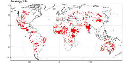
Figure 1: Locations of training sample plots. Each sample plot is 140 x 140 meters (approximately 2 hectares) with a 10 meter pixel size.

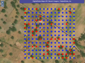
Figure 2: Screenshot from Collect Earth Online showing the plot labelling process. Red grid cells indicate the presence of a tree, while blue grid cells indicate the absence.

2.2 Model

The model consists of a fully convolutional neural network with a bidirectional convolutional gated recurrent unit (cGRU) encoder and a feature pyramid attention (FPA) decoder (Shi et al. 2015; Li et al. 2018) (Figure 3). The cGRU takes as input the biweekly processed Sentinel-1 and Sentinel-2 bands, and uses two-dimensional 3 x 3 convolutions to generate feature encodings that represent the per-pixel change over time. The FPA layer takes the local features generated by the cGRU and increases their field of view, incorporating knowledge about features from up to 15 pixels away, while maintaining the fine-grained localization of feature maps. This is done by multiplying deeper convolutional layers by a 1x1 convolutional layer. The upsampling blocks in the FPA layer use an upsize convolution rather than a transpose convolution in accordance with the recommendations in Odena, Dumoulin, and Olah (2016). These feature maps, which incorporate knowledge of both per-pixel and regional change over time, are then classified with a standard convolutional layer with a sigmoid activation.

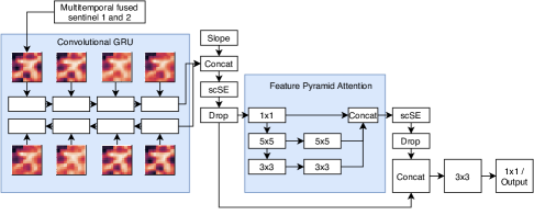
Figure 3: Overview of network architecture. Twenty-four input images for ten Sentinel-2, three indices, and two Sentinel-1 bands are passed to a bidirectional convolutional GRU to model temporal relationships. Next, the feature pyramid attention module integrates regional information with pixel-level information. Finally, Conv-BN-RELU-csSE-DropBlock blocks are combined with hypercolumns before sigmoid classification.

The cGRU layer uses layer normalization which standardizes features to avoid exploding gradients, and a channel squeeze and spatial excitation (SE) layer, which improves fine grained localization, between time steps (Ba, Kiros, and Hinton 2016; Roy, Navab, and Wachinger 2018). The SE block rescales each input channel c by multiplying by a sigmoid activated 1 x 1 x c convolution. Separate SE blocks are learned for the update and the reset gate of the GRU, respectively, and weights are shared between time steps.

The FPA layer is followed by two convolutional blocks with batch renormalization and csSE (Fig. 6) (Ioffe 2017; Roy, Navab, and Wachinger 2018). Hypercolumns, which concatenate deep and shallow features to increase layer dimension, are placed before the final sigmoid classification layer to facilitate pixel-level accuracy (Hariharan et al. 2014). The sigmoid bias layer was initialized in the same manner as in Lin et al. (2017) to avoid model collapse in the early stages of training. All padding operations in the model used reflect padding to enforce the distributional consistency of border convolutions. Weights were initialized according to He et al. (2015) when combined with batch renormalization, and glorot uniform otherwise (Glorot and Bengio 2010). Non-linear activations for intermediate layers use the rectified linear unit (RELU) (Nair and Hinton 2010). The ‘rmax’ and ‘dmax’ batch renormalization parameters follow the learning schedule in the original paper (Ioffe 2017). All experiments were conducted in Tensorflow 1.13.1 and the presented model has 221 thousand learnable parameters (Abadi et al. 2015). Data and code are released for reproducibility on the author’s GitHub page.

The model was optimized with the Adabound optimizer with learning rates between 1e-4 and 2e-2, and was trained for 100 epochs on a NVidia K80 GPU (Luo et al. 2019). A batch size of 20 was selected with equibatch sampling by tree cover percent (Berman and Blaschko 2017). To mitigate overfitting, several regularization methods were used. These include zoneout (prob = 0.2) in the GRU layer and dropblock (prob increases from 0 to 0.2 during training) after each intermediate convolutional layer (Krueger et al. 2016; Ghiasi, Lin, and Le 2018). The loss function for the model was a combination of label-smoothed (prob = 0.10) binary cross entropy, which was weighted by the effective number of samples, and the boundary loss (Szegedy et al. 2015; Cui et al. 2019; Kervadec et al. 2018). The weight of the boundary loss (BL) increased proportionate to the cross entropy loss (CE) throughout training according to Equation (4), where $y$ is the label segmentation, $p$ are the sigmoid probabilities, $\Omega$ is the spatial domain of $y$, and $\phi_{G}$ is a distance map with respect to the boundary of the positive segments of $y$.

$$\begin{split}\textrm{Loss}&=(1-\alpha)*\textrm{CE}+\alpha*\textrm{BL}\\ \alpha&=\textrm{Epoch}*0.01,\alpha\in[0.0,0.5]\\ \textrm{BL}&=\int_{\Omega}\phi_{G}(y)p_{\theta}(y)dy\\ \textrm{CE}&=-(y\textrm{log}(p\in[0.1,0.9])+(1-y)\textrm{log}(1-p\in[0.1,0.9]))\\ \end{split}$$ (4)

The model outputs were post-processed to improve accuracy around the border of input tiles by smoothing the predictions over a tiled window with two-dimensional interpolation between overlapping patches. The prediction for each pixel was calculated as the weighted average of nine input images, which were shifted either up, left, down, right, or diagonally by 70 meters from the original bounds, weighted by the distance of each pixel to the center of each of the nine input images with a Gaussian filter with a 3.5 pixel standard deviation. Prediction probabilities were converted to binary class labels based on a threshold determined by the receiver operating characteristic.

2.3 Validation Methods

Model performance was assessed at the global scale for pixel-level accuracy of tree identification and plot-level (140 x 140 meter) tree cover accuracy. Tree cover was calculated for each plot as the proportion of 10 x 10 meter pixels which were marked positive for tree presence in the same manner as in Bastin et al. (2017). Model performance was assessed for each decile of plot-level tree cover to identify comparative performance across different tree densities and distributions. In addition to the global validation methods, model performance was also tested for pixel and tree cover accuracy in three selected one million hectare landscapes in different biomes in Tanzania, Ghana, and Honduras. In all cases, accuracy validation was assessed against human-annotated high-resolution imagery, a method which has previously been used for accuracy assessments of wall-to-wall maps (Hansen et al. 2013; Zhang et al. 2019).

The proposed modelling approach was also tested against standard baselines, including random forests (RF), support vector machines (SVM), and a U-net CNN (Ronneberger, Fischer, and Brox 2015). The U-net is an often used CNN approach for remote sensing classification (Diakogiannis et al. 2019; Li et al. 2017). Baseline models were tested with different temporal aggregation methods, including mean, median, standard deviation, and quarterly and monthly mean composites. Both the random forests and the support vector machine baseline models use the mean band reflectance for each pixel over the 24 cloud-free images because this approach outperformed the other aggregation methods. The U-net baseline uses the median band reflectance. Common hyperparameters for each baseline approach were tuned using a brute force approach. The U-net CNN was designed in a similar manner to Ronneberger, Fischer, and Brox (2015), with the additions of reflect padding, batch renormalization, dropblock, and upsample convolution to match design choices of the proposed model. The U-net has 620 thousand trainable parameters and uses the Adabound optimizer with learning rates between 0.001 and 0.1.

2.3.1 Metrics

Model performance was evaluated with the user’s and producer’s accuracy. These metrics were modified in order to mitigate errors caused by variable coregistration consistency between WorldView 3 and Sentinel-2 imagery. Sub-pixel shifts in the Sentinel imagery are caused by resampling each image with nearest neighbor interpolation to fit within the plot boundaries due to the average coregistration error between images of 12 meters (Clerc 2020). Additionally, because WorldView 3 and Sentinel-2 have different viewing geometries and use different digital elevation models (DEM) for orthorectification, the products may be locally misaligned by more than ten meters (Kääb et al. 2016; Gašparović et al. 2019; Rumora et al. 2020). These local misalignments cause shifts between the WorldView 3 labels and the Sentinel predictions, rendering per-pixel metrics useless in many cases (Figure 4). To account for this, the producer’s accuracy counts false negatives (FN) if the ground truth positive occurs more than ten meters from a predicted positive at location $(x,y)$. Similarly, the user’s accuracy counts false positives (FP) if the predicted positive occurs more than ten meters from a positive ground truth pixel. There was no double counting of trees in either the ground truth or the predictions. The metrics are calculated according to Equation (5), where TP refers to true positives, $\hat{Y}$ refers to the prediction, and $Y$ refers to the label.

$$\begin{split}\textrm{User's acc}&=\dfrac{\textrm{TP}}{\textrm{TP + FP}}\\ \textrm{Producer's acc}&=\dfrac{\textrm{TP}}{\textrm{TP + FN}}\\ \textrm{TP}&=\sum_{x,y}\big{(}(Y_{x,y})(\max\hat{Y}_{x-1:x+1,y-1:y+1})\big{)}\\ \textrm{FP}&=\sum_{x,y}\big{(}(\hat{Y}_{x,y})(1-\max Y_{x-1:x+1,y-1:y+1})\big{)}\\ \textrm{FN}&=\sum_{x,y}\big{(}(Y_{x,y})(1-\max\hat{Y}_{x-1:x+1,y-1:y+1})\big{)}\end{split}$$ (5)

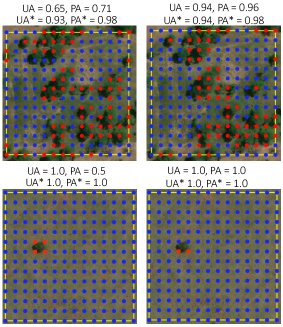
Figure 4: The user’s (UA) and producer’s accuracy (PA) are sensitive to labelling choices due to coregistration errors between Sentinel and WorldView imagery. Red pixels denote trees, blue pixels denote background. The labelling scheme on the left results in low UA and PA scores when analyzed with Sentinel imagery, despite being visually accurate. The labelling scheme on the right achieves high UA and PA scores. Both labelling schemes achieve similar UA and PA scores (denoted with *) when adjusted with Equation (5).

2.3.2 Global validation

Figure 5: Locations of testing sample plots. Each sample plot is 140 x 140 meters (approximately 2 hectares) with a 10 meter pixel size.

Pixel-level performance was assessed with 1,100 140 x 140 meter plots labelled in the same manner as the training data (section 2.1) (Figure 5). Seven hundred of the test plots were randomly distributed on land areas between -60 and +60 latitude. The other four hundred were randomly distributed within selected regions (including Central America, West Africa, East Africa, and India) to increase the ratio of test plots with high cloud cover and difficult land uses (such as plantation agriculture, agroforestry, step agriculture, and urbanization).

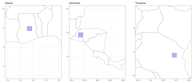
Figure 6: Locations of regional sample plots. Within each of the three regions, 100 evenly distributed 140 x 140 meter plots (represented with blue dots) were labelled with a 10 meter pixel size for binary tree presence. Additionally, within each of the three regions, a randomly selected 200 hectare sub-region was labelled with a 10 meter pixel size for binary tree presence.

To further assess model performance at the global scale, the percent tree cover of a random sub-sample of 1,000 half-hectare plots across global drylands from Bastin et al. (2017), stratified by geography and tree cover decile, were reanalyzed with recent high-resolution imagery (Figure 7). The percent tree cover was labeled in the same way as in Bastin et al. (2017), as the proportion of 10 meter pixels per plot that intersect a tree canopy. Thirty five percent of the reanalyzed plots disagreed with the labels in Bastin et al. (2017) by more than 30% tree cover. The labels for these plots were reassigned based on recent high-resolution imagery, while the rest retained their original labels. One source of disagreement was due to land use change since the original analysis. Because the plots were stratified by tree cover percent, plots with partial tree cover, were over-represented. These plots are also more likely to experience land use change than are plots with barren or dense canopy (Venter, Cramer, and Hawkins 2018; Kalamandeen et al. 2018). Another source of label disagreement arose from coregistration errors. Because more than half of 10-meter pixels in a half-hectare plot are border pixels, coregistration errors under 10 meters between the image analyzed in Bastin et al. (2017) and recent high-resolution imagery can alter tree cover predictions by up to 50%. Finally, Schepaschenko et al. (2017) identified significant classification error in the Bastin et al. (2017) data set due to old imagery and a lack of quality assurance. Tree density was calculated as the proportion of plot pixels with predictions higher than a threshold determined by the receiver operating characteristic.

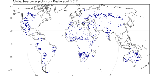
Figure 7: Locations of 1,000 half-hectare plots from Bastin et al. (2017) stratified by tree cover decile.

2.3.3 Regional validation

Model performance was also tested to ensure that the results for large geographic regions were consistent across different land uses and geographies. To do this, we prepared wall-to-wall maps of one million hectare regions in three geographies (Figure 6). The selected geographies included a Semi-arid desert with agricultural production in Tanzania, a tree Savannah with agricultural production in Ghana, and a mosaic tropical broad leaf forest landscape in Honduras. Model performance was assessed for these three regions through two complementary methods. To assess performance over the total one million hectares, 100 evenly distributed 140 x 140 meter plots were labelled in the same manner as in section 2.1. Additionally, to assess performance across smaller regions, a 200 hectare subregion was randomly identified for each of the three regions, for which each 10 meter pixel was labelled for binary tree presence. Combining these two validation sources, a total of 39,600 pixels were evaluated for each of the three regions. We also compare predictions with those of Zhang et al. (2019), who used a support vector machine to identify trees in 3 years of fused Sentinel-1 and Sentinel-2 imagery, with training data consisting of 20,000 labelled pixels in high-resolution imagery across the western Sahel.

3 Results

3.1 Global accuracy

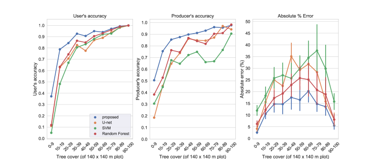
Figure 8: Performance of proposed model and baseline random forests (RF), support vector machine (SVM), and U-Net CNN measured with user’s and producer’s accuracy and the absolute percent error for each decile of plot-level tree cover.

Table 1: Per pixel confusion matrix, and user’s, producer’s, and overall accuracy for background and positive classes.

		Label
		No tree	Tree	Prod. Acc.
Pred	No tree	$133287$	$4802$	$96.5\%$
	Tree	$3599$	$74304$	$95.3\%$
	Usr. Acc.	$97.4\%$	$93.9\%$	$OA=96.1\%$

The proposed model is able to identify individual trees and small patches of trees across a variety of tree cover densities, land uses, biomes, terrains, and geographies. The model achieves 94% user’s accuracy and 95% producer’s accuracy across the 1,100 test plots, consisting of 215,600 pixels (Table 1)). When compared to the baseline random forest, support vector machine, and U-net, the proposed model performs substantially better in low tree cover scenarios, increasing user’s and producer’s accurracy by 33% and 24% over the best performing baseline model (U-net) in plots with below 20% tree cover (Figure 8; Table 2). For plots with between 20 and 40% tree cover, the proposed model increases user’s and producer’s accuracy by 9% and 13% over the best baseline model (random forest, Table 2).

Table 2: Performance of proposed model and baseline models in different geographical and biophysical conditions, measured with user’s and producer’s accuracy. RF = random forest, SVM = support vector machine.

	Proposed		RF		SVM		U-net
Parameter	User	Prod	User	Prod	User	Prod	User	Prod	n
Region
Africa	0.91	0.95	0.91	0.85	0.79	0.79	0.93	0.78	88,984
Asia	0.92	0.92	0.90	0.88	0.86	0.84	0.90	0.89	24,304
Australia	0.93	0.95	0.92	0.91	0.95	0.62	0.93	0.89	19,600
Europe	0.96	0.96	0.85	0.93	0.72	0.74	0.86	0.93	23,912
N. America	0.97	0.97	0.92	0.96	0.88	0.92	0.91	0.93	38,808
S. America	0.95	0.94	0.83	0.95	0.72	0.85	0.93	0.95	22,148
Cloud (%)
0-75	0.93	0.95	0.90	0.90	0.82	0.80	0.92	0.86	170,128
75+	0.94	0.95	0.89	0.92	0.82	0.86	0.91	0.91	45,864
Slope (%)
0-10	0.92	0.95	0.89	0.89	0.80	0.77	0.91	0.86	176,400
10+	0.97	0.95	0.91	0.95	0.86	0.92	0.93	0.91	39,592
Canopy (%)
0-20	0.66	0.60	0.27	0.47	0.14	0.39	0.33	0.36	115,248
20-40	0.88	0.87	0.79	0.75	0.72	0.66	0.76	0.69	21,560
40-60	0.90	0.93	0.88	0.85	0.86	0.74	0.83	0.85	11,956
60-100	0.97	0.99	0.99	0.96	0.99	0.86	0.99	0.93	67,228
Overall	0.94	0.95	0.90	0.91	0.81	0.82	0.91	0.88	215,992

Across all testing plots, the proposed model improves the mean tree cover error to 7.1% (6.4 - 7.9%, 95% CI) from 10.7% (8.7 - 11.6%, random forest). In plots with between 30 and 70% tree cover, the percent tree cover error is reduced from 22.6% (20.0 - 25.1%) to 16.7% (14.6 - 18.8%) (Figure 8). The proposed model is not sensitive to cloud cover or steep terrain. In very cloudy test plots (at least 75% of imagery dates with at least 20% cloud cover), the proposed model maintains high accuracy, with 95 and 94% user’s and producer’s accuracy, reducing omission and commission errors against the baseline models by almost half (Table 2). Different methods of temporal aggregation did not considerably change the accuracy metrics for the baseline models (Table 3).

Table 3: Performance of baseline models with different temporal aggregation methods. Bold numbers indicate the selected aggregation method for the associated model. S.D. = standard deviation.

	Random Forest		SVM		U-net
Aggregation	User	Prod.	User	Prod.	User	Prod.
Mean	0.90	0.91	0.81	0.82	0.91	0.88
Median	0.91	0.90	0.81	0.80	0.92	0.88
Mean + S.D.	0.89	0.90	0.82	0.81	0.90	0.90
Median + S.D.	0.89	0.91	0.81	0.81	0.90	0.91
Quarterly mean	0.90	0.90	0.81	0.81	0.91	0.86
Monthly mean	0.89	0.90	0.82	0.81	0.91	0.88

The predicted tree cover for the 1,000 stratified plot locations from Bastin et al. (2017) had an average of 0.85 (0.83-0.86, 95% CI) Pearson’s correlation with the cleaned tree cover labels from Bastin et al. (2017). The Pearson’s correlation for the random forest model was 0.76 (0.74-0.79, 95% CI) and for the U-net was 0.77 (0.74-0.79, 95% CI). The proposed model classified above and below 10% tree cover with 92% and 91% user’s and producer’s accuracy, compared to random forest (90%, 82%, respectively) and U-net (92%, 85%, respectively) (Figure 9).

Figure 9: Confusion matrix of predicted versus labeled tree cover from Bastin et al. (2017) for the proposed model, random forest, and U-net.

3.2 Regional accuracy

Table 4: User’s and producer’s accuracy for the selected one million ha regions and 200 ha subregions in Ghana, Tanzania, and Honduras.

	Proposed model		Random Forest		U-net
Parameter	User	Prod.	User	Prod.	User	Prod.
Ghana - region	0.80	0.82	0.77	0.77	0.70	0.70
Ghana - subregion	0.81	0.76	0.78	0.75	0.75	0.76
Tanzania - region	0.86	0.84	0.75	0.78	0.74	0.84
Tanzania - subregion	0.85	0.84	0.52	0.54	0.76	0.75
Honduras - region	0.99	0.98	0.97	0.97	0.96	0.95
Honduras - subregion	0.94	0.99	0.93	0.99	0.92	0.97

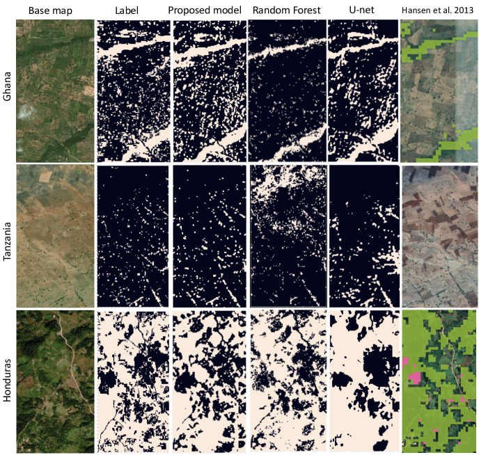
Figure 10: Predictions of the proposed model and baselines for the 200 hectare subregions in Ghana, Tanzania, and Honduras, along with the labels, based on high-resolution imagery, and the high-resolution base map. Predictions of Hansen et al. (2013) are added for reference, where green pixels indicate tree cover, and pink pixels indicate tree cover loss.

The proposed model achieves an average of 87.5% user’s accuracy and 87.2% producer’s accuracy across the 118,800 labelled pixels in Ghana, Tanzania, and Honduras. This reflects a 7.2% and 7.3% increase over the random forests, and a 7% and 4.2% increase over the U-net in terms of user’s and producer’s accuracy (Table 4).

In the 200 hectare subregion in Ghana, the proposed model accurately locates both the scattered trees on farm land and the tree corridors (Figure 10). In comparison, the random forest misses the majority of the scattered trees on farm land, while the U-net overpredicts the density of large patches of trees, and completely misses many small patches of trees. Overall, the proposed model reduces relative commission and omission error by 13% and 22% versus the random forest, and 33% and 40% versus the U-net for the larger region.

The proposed model is able to locate most individual trees in the 200 hectare subregion in Tanzania (Figure 10). The random forest model only detected large patches of trees, and the U-net again over-predicted the density of large patches while missing most of the individual trees. When compared to the baseline random forest model, the proposed model reduces relative commission and omission error by 63% and 27% for the larger region, and commission error by 46% versus the U-net.

Figure 11: Performance comparisons with results from Zhang et al. (2019) for a 42 hectare region in Senegal. Labels from Brandt et al. (2018) are denoted in green and predictions are denoted in magenta. The proposed model identifies 85% of the trees labeled in Brandt et al. (2018).

In the 200 hectare subregion in Honduras, the proposed model identified most of the small patches of barren land within the surrounding dense tree cover, while also identifying many of the individual trees that on farmland (Figure 10). In comparison, the random forest’s predictions were very noisy around the boundaries between dense and scattered tree cover, and the individual trees on farmland were not identified. The U-net was unable to identify the small patches of barren land, and overestimated tree cover substantially. When visually compared with the results from Hansen et al. (2013), the proposed model performs much better at identifying scattered trees, while Hansen et al. (2013) performs visually similar for trees inside closed-canopy forests (Figure 10). Compared to the predictions of Zhang et al. (2019), the proposed model improves accuracy by 50% from 35% to 85% in a 42 hectare region of Senegal (Figure 11).

4 Discussion

4.1 Implications for global forest monitoring efforts

Global assessments of tree cover have underestimated tree cover extent in drylands as well as scattered tree cover in urban environments and mosaic landscapes (Bastin et al. 2017; Ottosen et al. 2020; Milodowski, Mitchard, and Williams 2017). This has caused considerable uncertainty in estimating the extent of these forms of tree cover at a global scale. Through human photointerpretation of 500,000 plots with high-resolution satellite imagery, Bastin et al. (2017) found that global remote sensing classifiers underestimated dryland forest extent by 40%. With regard to trees on cropland, Zomer et al. (2016) found that more than 40% of cropland on earth has at least 10% canopy cover. However, without a globally consistent and efficient method to measure these types of sparse and scattered tree cover, estimates continue to rely either on aggregating data from multiple, small-scale assessments, or on human photointerpretation.

The methodology presented in this paper enables the assessment of sparse and scattered tree cover with medium-resolution satellite imagery. The accuracy of monitoring tree presence in highly heterogeneous areas such as those with sparse and scattered tree cover was improved by as much as 20% over standard remote sensing classifiers such as random forests and support vector machines. Additionally, the proposed approach reduces omission and commission errors in dense tree cover, high cloud cover, and mountainous regions by nearly half compared to standard remote sensing classifiers. Global data that combines contiguous, closed-canopy forest extent with tree cover data in low tree cover regions will have significant implications for global land use and land change monitoring.

Many types and drivers of land use change, such as small area deforestation, encroachment, habitat fragmentation, and natural regeneration, occur primarily in highly heterogeneous regions like the urban fringe, forest perimeters, and riparian zones (Tyukavina et al. 2018; Venter, Cramer, and Hawkins 2018; Pickett and Cadenasso 1995; Rex and Malanson 1990). For instance, the majority of woody encroachment into open areas in continental Africa occurs in regions with moderate initial tree cover (between 30 - 60%) (Venter, Cramer, and Hawkins 2018). Furthermore, more than two thirds of deforestation in both the Congo basin and the Amazon between 2000 and 2014 was driven by smallholder clearing (Kalamandeen et al. 2018). Human-driven increases in canopy cover, such as afforestation and reforestation, also tend to be comprised of many small tree planting efforts, often by individual land owners (Holl 2017; Melo et al. 2013). These highly heterogeneous regions where important land use changes are occurring are known to have lower classification accuracy for tree cover and land use than larger, homogeneous regions in many remote sensing approaches (Smith et al. 2002; Milodowski, Mitchard, and Williams 2017; Vasconcelos 2018). This limits the applicability of existing global tree cover datasets to monitor small area deforestation, natural regeneration, and landscape restoration.

More than 50 countries have committed to putting more than 170 million hectares of land under restoration by 2030 (FAO and WRI 2019). Restoration land use interventions target open-canopy forests and trees outside of forests, including agroforestry, silviculture, and natural regeneration. While global data like that of Hansen et al. (2013) have transformed forest monitoring and carbon accounting, there is no comparable global method or data to monitor progress on restoration. Instead, restoration monitoring programs are generally constructed at the national or landscape scale, and rely on field data and human interpretation of satellite imagery (Bey et al. 2016; Tumeo et al. 2018). The methodological improvements for tree identification in areas with sparse and scattered tree cover presented in this paper may allow for increased spatial and temporal resolution of monitoring data for land use management decisions by reducing reliance on photointerpretation and field data.

4.2 Implications for remote sensing methodologies

The applications of deep learning methodologies such as CNNs to medium-resolution remote sensing imagery are not well understood. The majority of classification systems rely on random forests or support vector machines rather than CNNs (Ma et al. 2019). Indeed, in the present study, the U-net baseline performed similarly to the random forest, despite being more than an order of magnitude more computationally intensive. Many studies have concluded that the U-net significantly outperforms other machine learning classifiers for remote sensing tasks with high-resolution imagery (Diakogiannis et al. 2019; Li et al. 2017; Feng et al. 2019; Xu et al. 2018; Zhang, Liu, and Wang 2018). The relative underperformance of the U-net with medium-resolution imagery highlights a need for alternative CNN approaches such as the one proposed in this paper.

By explicitly designing the model architecture to mitigate the constraints of medium-resolution data, the proposed model was able to significantly outperform the U-net model and the other machine learning baselines in every decile of tree cover (Figure 8). These design choices included increasing data complexity with temporal data and the convolutional GRU, choosing model building blocks that are explicitly designed for pixel-level accuracy (FPA, csSE), and using a loss function explicitly designed for different tree cover scenarios and coregistration errors (boundary loss and label smoothing). Because the improvements in accuracy are rooted in the temporal CNN architecture, it is likely that the proposed model design could also greatly benefit land use modeling and the identification of objects in satellite imagery such as roofs, power plants, boats, or roads.

4.3 Future research

Despite the numerous improvements presented in this paper, there are several avenues for future research in imagery preprocessing that could further improve accuracy in low tree cover regions. Due to the global nature of this work, the present approach naively fuses Sentinel-1 and Sentinel-2 by simply stacking the Sentinel-1 ground range detected (GRD) product with the Sentinel-2 L2A product. Because of the sub-pixel size of trees in Sentinel imagery, the pixel-level match up between Sentinel-1 and Sentinel-2 is very important for reducing the blurriness of predictions. Many new approaches for fusing Sentinel-1 and Sentinel-2 have recently been proposed, such as probabilistic Bayesian models, affine transformations, and CNN-based approaches (Fernandez-Beltran et al. 2018; Benedetti, Picchiani, and Del Frate 2018). While these approaches are often limited to small geographies and their benefit to global-scale preprocessing is not yet clear, increasing the pixel-level accuracy of Sentinel-1 and 2 fusion would likely improve the identification of small tree patches.

Because the proposed model uses multitemporal imagery, the interpolation of cloud and cloud shadow pixels is very important to accurately reconstruct imagery, especially when the gap between cloud-free image acquisitions is substantial. Although the proposed model in this paper performs much better than the baseline models in high cloud cover scenarios, there is room to improve the interpolation of cloud and cloud shadow when constructing time series imagery. The presented methodology uses the Whittaker smoother, which Kandasamy et al. (2013) found to be better at interpolating time series gaps in MODIS imagery in comparison to temporal smoothing and gap filling, Gaussian functions, low pass filters, and many other per-pixel smoothing functions. In contrast to these per-pixel approaches, a number of spatio-temporal methods for gap filling have been proposed. Such methods include conditional generative adversarial networks (Xia et al. 2019), convolutional neural networks (Zhang et al. 2020), patch-based cloning (Lin et al. 2013), k-nearest neighbors (Malambo and Heatwole 2016), and spatio-temporal Markov random fields (Cheng et al. 2014).

Finally, future research should identify the benefits of the proposed model for change detection, such as identifying small-scale deforestation as well as forest and landscape restoration activities. While the present paper demonstrates comparative benefits over commonly used remote sensing classifiers for tree identification in heterogeneous landscapes, the potential benefits for change detection are left to future work. In a similar manner, future research should detail how the methodology presented in this paper can be integrated into national and subnational environmental monitoring programs. One potential avenue is through human-in-the-loop artificial intelligence, where locally generated data is used to improve the local accuracy of globally developed models (Logar et al. 2020). Because neural networks allow for online learning, they can easily be ’fine-tuned’ with new data, while models such as random forests and support vector machines cannot (Zhou et al. 2017). This allows for the combination of participatory mapping and crowd sourcing, where local stakeholders label high-resolution imagery with the power of neural network based remote sensing classifiers.

References

- Abadi et al. (2015) Abadi, Martín, Ashish Agarwal, Paul Barham, Eugene Brevdo, Zhifeng Chen, Craig Citro, Greg S. Corrado, et al. 2015. “TensorFlow: Large-Scale Machine Learning on Heterogeneous Systems.” Software available from tensorflow.org, http://tensorflow.org/.
- Ba, Kiros, and Hinton (2016) Ba, Jimmy Lei, Jamie Ryan Kiros, and Geoffrey E. Hinton. 2016. “Layer Normalization.” .
- Bastin et al. (2017) Bastin, Jean-François, Nora Berrahmouni, Alan Grainger, Danae Maniatis, Danilo Mollicone, Rebecca Moore, Chiara Patriarca, et al. 2017. “The extent of forest in dryland biomes.” Science 356 (6338): 635–638. https://science.sciencemag.org/content/356/6338/635.
- Benedetti, Picchiani, and Del Frate (2018) Benedetti, A., M. Picchiani, and F. Del Frate. 2018. “Sentinel-1 and Sentinel-2 Data Fusion for Urban Change Detection.” In IGARSS 2018 - 2018 IEEE International Geoscience and Remote Sensing Symposium, 1962–1965.
- Berman and Blaschko (2017) Berman, Maxim, and Matthew B. Blaschko. 2017. “Optimization of the Jaccard index for image segmentation with the Lovász hinge.” CoRR abs/1705.08790. http://arxiv.org/abs/1705.08790.
- Bey et al. (2016) Bey, Adia, Alfonso Sánchez-Paus Díaz, Danae Maniatis, Giulio Marchi, Danilo Mollicone, Stefano Ricci, Jean-François Bastin, et al. 2016. “Collect Earth: Land Use and Land Cover Assessment through Augmented Visual Interpretation.” Remote Sensing 8: 807.
- Bolyn et al. (2018) Bolyn, Corentin, Adrien Michez, Peter Gaucher, Philippe Lejeune, and Stéphanie Bonnet. 2018. “Forest mapping and species composition using supervised per pixel classification of Sentinel-2 imagery.” .
- Brandt et al. (2018) Brandt, Martin, Kjeld Rasmussen, Pierre Hiernaux, Stefanie Herrmann, Compton Tucker, Xiaoye Tong, Feng Tian, et al. 2018. “Reduction of tree cover in West African woodlands and promotion in semi-arid farmlands.” Nature Geoscience 11.
- Candra, Phinn, and Scarth (2020) Candra, Danang Surya, Stuart Phinn, and Peter Scarth. 2020. “Cloud and cloud shadow masking for Sentinel-2 using multitemporal images in global area.” International Journal of Remote Sensing 41 (8): 2877–2904. https://doi.org/10.1080/01431161.2019.1697006.
- Castelluccio et al. (2015) Castelluccio, Marco, Giovanni Poggi, Carlo Sansone, and Luisa Verdoliva. 2015. “Land Use Classification in Remote Sensing Images by Convolutional Neural Networks.” ArXiv abs/1508.00092.
- Cheng et al. (2014) Cheng, Qing, Huanfeng Shen, Liangpei Zhang, Qiangqiang Yuan, and Chao Zeng. 2014. “Cloud removal for remotely sensed images by similar pixel replacement guided with a spatio-temporal MRF model.” ISPRS Journal of Photogrammetry and Remote Sensing 92: 54 – 68. http://www.sciencedirect.com/science/article/pii/S0924271614000537.
- Clerc (2020) Clerc, Sebastian. 2020. Sentinel 2 L1C Data Quality Report. Technical Report 50. ESA.
- Cui et al. (2019) Cui, Yin, Menglin Jia, Tsung-Yi Lin, Yang Song, and Serge J. Belongie. 2019. “Class-Balanced Loss Based on Effective Number of Samples.” CoRR abs/1901.05555. http://arxiv.org/abs/1901.05555.
- Diakogiannis et al. (2019) Diakogiannis, Foivos I., François Waldner, Peter Caccetta, and Chen Wu. 2019. “ResUNet-a: a deep learning framework for semantic segmentation of remotely sensed data.” CoRR abs/1904.00592. http://arxiv.org/abs/1904.00592.
- Eilers (2003) Eilers, Paul H. C. 2003. “A Perfect Smoother.” Analytical Chemistry 75 (14): 3631–3636. PMID: 14570219, https://doi.org/10.1021/ac034173t.
- FAO (2015) FAO. 2015. Global Forest Resources Assessment 2015.
- FAO and WRI (2019) FAO, and WRI. 2019. The Road to Restoration: A Guide to Identifying Priorities and Indicators for Monitoring Forest and Landscape Restoration.
- Feng et al. (2019) Feng, W., H. Sui, W. Huang, C. Xu, and K. An. 2019. “Water Body Extraction From Very High-Resolution Remote Sensing Imagery Using Deep U-Net and a Superpixel-Based Conditional Random Field Model.” IEEE Geoscience and Remote Sensing Letters 16 (4): 618–622.
- Fernandez-Beltran et al. (2018) Fernandez-Beltran, R., J. M. Haut, M. E. Paoletti, J. Plaza, A. Plaza, and F. Pla. 2018. “Multimodal Probabilistic Latent Semantic Analysis for Sentinel-1 and Sentinel-2 Image Fusion.” IEEE Geoscience and Remote Sensing Letters 15 (9): 1347–1351.
- Gašparović et al. (2019) Gašparović, Mateo, Luka Rumora, Mario Miler, and Damir Medak. 2019. “Effect of fusing Sentinel-2 and WorldView-4 imagery on the various vegetation indices.” Journal of Applied Remote Sensing 13 (3): 1 – 18. https://doi.org/10.1117/1.JRS.13.036503.
- Ghiasi, Lin, and Le (2018) Ghiasi, Golnaz, Tsung-Yi Lin, and Quoc V. Le. 2018. “DropBlock: A Regularization Method for Convolutional Networks.” In Proceedings of the 32nd International Conference on Neural Information Processing Systems, NIPS’18, Red Hook, NY, USA, 10750–10760. Curran Associates Inc.
- Glorot and Bengio (2010) Glorot, Xavier, and Y. Bengio. 2010. “Understanding the difficulty of training deep feedforward neural networks.” Journal of Machine Learning Research - Proceedings Track 9: 249–256.
- Goodfellow, Bengio, and Courville (2016) Goodfellow, Ian, Yoshua Bengio, and Aaron Courville. 2016. Deep Learning. MIT Press.
- Hansen et al. (2013) Hansen, M. C., P. V. Potapov, R. Moore, M. Hancher, S. A. Turubanova, A. Tyukavina, D. Thau, et al. 2013. “High-Resolution Global Maps of 21st-Century Forest Cover Change.” Science 342 (6160): 850–853. https://science.sciencemag.org/content/342/6160/850.
- Hariharan et al. (2014) Hariharan, Bharath, Pablo Arbeláez, Ross Girshick, and Jitendra Malik. 2014. “Hypercolumns for Object Segmentation and Fine-grained Localization.” .
- He et al. (2015) He, Kaiming, Xiangyu Zhang, Shaoqing Ren, and Jian Sun. 2015. “Delving Deep into Rectifiers: Surpassing Human-Level Performance on ImageNet Classification.” CoRR abs/1502.01852. http://arxiv.org/abs/1502.01852.
- Holl (2017) Holl, Karen D. 2017. “Restoring tropical forests from the bottom up.” Science 355 (6324): 455–456. https://science.sciencemag.org/content/355/6324/455.
- Hościło and Lewandowska (2019) Hościło, Agata, and Aneta Lewandowska. 2019. “Mapping Forest Type and Tree Species on a Regional Scale Using Multi-Temporal Sentinel-2 Data.” Remote Sensing 11 (8): 929. http://dx.doi.org/10.3390/rs11080929.
- Ibtehaz and Rahman (2020) Ibtehaz, Nabil, and M. Sohel Rahman. 2020. “MultiResUNet : Rethinking the U-Net architecture for multimodal biomedical image segmentation.” Neural Networks 121: 74 – 87. http://www.sciencedirect.com/science/article/pii/S0893608019302503.
- Immitzer, Vuolo, and Atzberger (2016) Immitzer, Markus, Francesco Vuolo, and Clement Atzberger. 2016. “First Experience with Sentinel-2 Data for Crop and Tree Species Classifications in Central Europe.” Remote Sensing 8: 166.
- Ioffe (2017) Ioffe, Sergey. 2017. “Batch Renormalization: Towards Reducing Minibatch Dependence in Batch-Normalized Models.” .
- Jiang et al. (2008) Jiang, Zhangyan, Alfredo R. Huete, Kamel Didan, and Tomoaki Miura. 2008. “Development of a two-band enhanced vegetation index without a blue band.” Remote Sensing of Environment 112 (10): 3833 – 3845. http://www.sciencedirect.com/science/article/pii/S0034425708001971.
- Kalamandeen et al. (2018) Kalamandeen, M, E Gloor, E Mitchard, D Quincey, G Ziv, D Spracklen, B Spracklen, M Adami, LEOC Aragaõ, and D Galbraith. 2018. “Pervasive Rise of Small-scale Deforestation in Amazonia.” Scientific Reports 8. http://eprints.whiterose.ac.uk/127554/.
- Kandasamy et al. (2013) Kandasamy, Sivasathivel, Baret Frederic, A. Verger, Ph Neveux, and Marie Weiss. 2013. “A comparison of methods for smoothing and gap filling time series of remote sensing observations: Application to MODIS LAI products.” Biogeosciences 10: 4055–4071.
- Kervadec et al. (2018) Kervadec, Hoel, Jihene Bouchtiba, Christian Desrosiers, Éric Granger, Jose Dolz, and Ismail Ben Ayed. 2018. “Boundary loss for highly unbalanced segmentation.” .
- Kim et al. (2014) Kim, Do-Hyung, Joseph O. Sexton, Praveen Noojipady, Chengquan Huang, Anupam Anand, Saurabh Channan, Min Feng, and John R. Townshend. 2014. “Global, Landsat-based forest-cover change from 1990 to 2000.” Remote Sensing of Environment 155: 178 – 193. http://www.sciencedirect.com/science/article/pii/S0034425714003149.
- Krueger et al. (2016) Krueger, David, Tegan Maharaj, János Kramár, Mohammad Pezeshki, Nicolas Ballas, Nan Rosemary Ke, Anirudh Goyal, et al. 2016. “Zoneout: Regularizing RNNs by Randomly Preserving Hidden Activations.” CoRR abs/1606.01305. http://arxiv.org/abs/1606.01305.
- Kääb et al. (2016) Kääb, Andreas, Solveig Winsvold, Bas Altena, Christopher Nuth, Thomas Nagler, and Jan Wuite. 2016. “Glacier Remote Sensing Using Sentinel-2. Part I: Radiometric and Geometric Performance, and Application to Ice Velocity.” Remote Sensing 8 (7): 598. http://dx.doi.org/10.3390/rs8070598.
- Lal (2002) Lal, R. 2002. “Soil carbon sequestration in China through agricultural intensification, and restoration of degraded and desertified ecosystems.” Land Degradation & Development 13 (6): 469–478. https://onlinelibrary.wiley.com/doi/abs/10.1002/ldr.531.
- Lanaras et al. (2018) Lanaras, Charis, José M. Bioucas-Dias, Silvano Galliani, Emmanuel Baltsavias, and Konrad Schindler. 2018. “Super-Resolution of Sentinel-2 Images: Learning a Globally Applicable Deep Neural Network.” CoRR abs/1803.04271. http://arxiv.org/abs/1803.04271.
- Li et al. (2018) Li, Hanchao, Pengfei Xiong, Jie An, and Lingxue Wang. 2018. “Pyramid Attention Network for Semantic Segmentation.” .
- Li et al. (2017) Li, Ruirui, Wenjie Liu, Lei Yang, Shihao Sun, W. H. Hu, Fan Zhang, and Wei Li. 2017. “DeepUNet: A Deep Fully Convolutional Network for Pixel-Level Sea-Land Segmentation.” IEEE Journal of Selected Topics in Applied Earth Observations and Remote Sensing 11: 3954–3962.
- Li (2014) Li, Sufen. 2014. “A NEW BARE-SOIL INDEX FOR RAPID MAPPING DEVELOPING AREAS USING LANDSAT 8 DATA.” .
- Lin et al. (2013) Lin, C., P. Tsai, K. Lai, and J. Chen. 2013. “Cloud Removal From Multitemporal Satellite Images Using Information Cloning.” IEEE Transactions on Geoscience and Remote Sensing 51 (1): 232–241.
- Lin et al. (2017) Lin, Tsung-Yi, Priya Goyal, Ross B. Girshick, Kaiming He, and Piotr Dollár. 2017. “Focal Loss for Dense Object Detection.” CoRR abs/1708.02002. http://arxiv.org/abs/1708.02002.
- Logar et al. (2020) Logar, Tomaz, Joseph Bullock, Edoardo Nemni, Lars Bromley, John A. Quinn, and Miguel Luengo-Oroz. 2020. “PulseSatellite: A tool using human-AI feedback loops for satellite image analysis in humanitarian contexts.” .
- Luo et al. (2019) Luo, Liangchen, Yuanhao Xiong, Yan Liu, and Xu Sun. 2019. “Adaptive Gradient Methods with Dynamic Bound of Learning Rate.” .
- Ma et al. (2019) Ma, Lei, Yu Liu, Xueliang Zhang, Yuanxin Ye, Gaofei Yin, and Brian Alan Johnson. 2019. “Deep learning in remote sensing applications: A meta-analysis and review.” ISPRS Journal of Photogrammetry and Remote Sensing 152: 166 – 177. http://www.sciencedirect.com/science/article/pii/S0924271619301108.
- Malambo and Heatwole (2016) Malambo, L., and C. D. Heatwole. 2016. “A Multitemporal Profile-Based Interpolation Method for Gap Filling Nonstationary Data.” IEEE Transactions on Geoscience and Remote Sensing 54 (1): 252–261.
- Manakos, Kordelas, and Marini (2019) Manakos, Ioannis, Georgios A. Kordelas, and Kalliroi Marini. 2019. “Fusion of Sentinel-1 data with Sentinel-2 products to overcome non-favourable atmospheric conditions for the delineation of inundation maps.” European Journal of Remote Sensing 0 (0): 1–14. https://doi.org/10.1080/22797254.2019.1596757.
- Melo et al. (2013) Melo, Felipe P.L., Severino R.R. Pinto, Pedro H.S. Brancalion, Pedro S. Castro, Ricardo R. Rodrigues, James Aronson, and Marcelo Tabarelli. 2013. “Priority setting for scaling-up tropical forest restoration projects: Early lessons from the Atlantic Forest Restoration Pact.” Environmental Science and Policy 33: 395 – 404. http://www.sciencedirect.com/science/article/pii/S1462901113001494.
- Milodowski, Mitchard, and Williams (2017) Milodowski, D T, E T A Mitchard, and M Williams. 2017. “Forest loss maps from regional satellite monitoring systematically underestimate deforestation in two rapidly changing parts of the Amazon.” Environmental Research Letters 12 (9): 094003. https://doi.org/10.1088%2F1748-9326%2Faa7e1e.
- Nair and Hinton (2010) Nair, Vinod, and Geoffrey E. Hinton. 2010. “Rectified Linear Units Improve Restricted Boltzmann Machines.” In ICML, .
- Odena, Dumoulin, and Olah (2016) Odena, Augustus, Vincent Dumoulin, and Chris Olah. 2016. “Deconvolution and Checkerboard Artifacts.” Distill http://distill.pub/2016/deconv-checkerboard.
- Ottosen et al. (2020) Ottosen, Thor-Bjørn, Geoffrey Petch, Mary Hanson, and Carsten A. Skjøth. 2020. “Tree cover mapping based on Sentinel-2 images demonstrate high thematic accuracy in Europe.” International Journal of Applied Earth Observation and Geoinformation 84: 101947. http://www.sciencedirect.com/science/article/pii/S0303243419306087.
- Pickett and Cadenasso (1995) Pickett, S. T. A., and M. L. Cadenasso. 1995. “Landscape Ecology: Spatial Heterogeneity in Ecological Systems.” Science 269 (5222): 331–334. https://science.sciencemag.org/content/269/5222/331.
- Qi, Kerr, and Chehbouni (1994) Qi, Jiaguo, Yann H. Kerr, and Abdelghani Chehbouni. 1994. “External factor consideration in vegetation index development.” .
- Radoux et al. (2016) Radoux, Julien, Guillaume Chomé, Damien Jacques, François Waldner, Nicolas Bellemans, Nicolas Matton, Céline Lamarche, Raphaël d’Andrimont, and Pierre Defourny. 2016. “Sentinel-2’s Potential for Sub-Pixel Landscape Feature Detection.” Remote Sensing 8 (6): 488.
- Rex and Malanson (1990) Rex, K. D., and George P. Malanson. 1990. “The fractal shape of riparian forest patches.” Landscape Ecology 4: 249–258.
- Rodriguez and Wegner (2018) Rodriguez, Andres C., and Jan Dirk Wegner. 2018. “Counting the uncountable: deep semantic density estimation from Space.” CoRR abs/1809.07091. http://arxiv.org/abs/1809.07091.
- Ronneberger, Fischer, and Brox (2015) Ronneberger, Olaf, Philipp Fischer, and Thomas Brox. 2015. “U-Net: Convolutional Networks for Biomedical Image Segmentation.” CoRR abs/1505.04597. http://arxiv.org/abs/1505.04597.
- Roy, Navab, and Wachinger (2018) Roy, Abhijit Guha, Nassir Navab, and Christian Wachinger. 2018. “Concurrent Spatial and Channel Squeeze and Excitation in Fully Convolutional Networks.” .
- Roy and Inamdar (2019) Roy, Anjan, and Arun Inamdar. 2019. “Multi-temporal Land Use Land Cover (LULC) change analysis of a dry semi-arid river basin in western India following a robust multi-sensor satellite image calibration strategy.” In Heliyon, .
- Rumelhart, Hinton, and Williams (1988) Rumelhart, David E., Geoffrey E. Hinton, and Ronald J. Williams. 1988. Learning Representations by Back-Propagating Errors, 696–699. Cambridge, MA, USA: MIT Press.
- Rumora et al. (2020) Rumora, Luka, Mateo Gašparović, Mario Miler, and Damir Medak. 2020. “Quality assessment of fusing Sentinel-2 and WorldView-4 imagery on Sentinel-2 spectral band values: a case study of Zagreb, Croatia.” International Journal of Image and Data Fusion 11 (1): 77–96. https://doi.org/10.1080/19479832.2019.1683624.
- Rußwurm and Körner (2018) Rußwurm, Marc, and Marco Körner. 2018. “Multi-Temporal Land Cover Classification with Sequential Recurrent Encoders.” CoRR abs/1802.02080. http://arxiv.org/abs/1802.02080.
- Saah et al. (2019) Saah, David, Gary Johnson, Billy Ashmall, Githika Tondapu, Karis Tenneson, Matt Patterson, Ate Poortinga, et al. 2019. “Collect Earth: An online tool for systematic reference data collection in land cover and use applications.” Environmental Modelling and Software 118: 166 – 171. http://www.sciencedirect.com/science/article/pii/S1364815218312568.
- Schepaschenko et al. (2017) Schepaschenko, Dmitry, Steffen Fritz, Linda See, Juan Laso Bayas, Myroslava Lesiv, Florian Kraxner, and Michael Obersteiner. 2017. “Comment on “The extent of forest in dryland biomes”.” Science 358: eaao0166.
- Schnell et al. (2014) Schnell, Sebastian, Dan Altrell, Göran Ståhl, and Christoph Kleinn. 2014. “The contribution of trees outside forests to national tree biomass and carbon stocks—a comparative study across three continents.” Environmental Monitoring and Assessment 187: 1–18.
- Schnell, Kleinn, and Ståhl (2015) Schnell, Sebastian, Christoph Kleinn, and Göran Ståhl. 2015. “Monitoring trees outside forests: a review.” Environmental Monitoring and Assessment 187.
- Shi et al. (2015) Shi, Xingjian, Zhourong Chen, Hao Wang, Dit-Yan Yeung, Wai-kin Wong, and Wang-chun Woo. 2015. “Convolutional LSTM Network: A Machine Learning Approach for Precipitation Nowcasting.” Cite arxiv:1506.04214, http://arxiv.org/abs/1506.04214.
- Smeets (2007) Smeets, Edward. 2007. “Bioenergy potentials from forestry in 2050.” Climatic Change 81: 353–390.
- Smith et al. (2002) Smith, Jonathan D. H., James D. Wickham, Stephen V. Stehman, and Limin Yang. 2002. “IMPACTS OF PATCH SIZE AND LAND-COVER HETEROGENEITY ON THEMATIC IMAGE CLASSIFICATION ACCURACY.” .
- Szegedy et al. (2015) Szegedy, Christian, Vincent Vanhoucke, Sergey Ioffe, Jonathon Shlens, and Zbigniew Wojna. 2015. “Rethinking the Inception Architecture for Computer Vision.” CoRR abs/1512.00567. http://arxiv.org/abs/1512.00567.
- Tavares et al. (2019) Tavares, Paulo, Norma Beltrão, Ulisses Guimarães, and A. Teodoro. 2019. “Integration of Sentinel-1 and Sentinel-2 for Classification and LULC Mapping in the Urban Area of Belém, Eastern Brazilian Amazon.” Sensors 19.
- Tumeo et al. (2018) Tumeo, T., C. Chilima, K. Reytar, S. Ray, L. Toh, and R. Kaanan. 2018. A Framework for Monitoring Progress On Malawi’s National Forest Landscapes Restoration Strategy.
- Tyukavina et al. (2018) Tyukavina, Alexandra, Matthew C. Hansen, Peter Potapov, Diana Parker, Chima Okpa, Stephen V. Stehman, Indrani Kommareddy, and Svetlana Turubanova. 2018. “Congo Basin forest loss dominated by increasing smallholder clearing.” Science Advances 4 (11). https://advances.sciencemag.org/content/4/11/eaat2993.
- Vasconcelos (2018) Vasconcelos, Maria. 2018. “Striking divergences in Earth Observation products may limit their use for REDD+.” Environmental Research Letters 13.
- Venter, Cramer, and Hawkins (2018) Venter, Zander, Michael Cramer, and Heidi Hawkins. 2018. “Drivers of woody plant encroachment over Africa.” Nature Communications 9.
- Xia et al. (2019) Xia, Y., H. Zhang, L. Zhang, and Z. Fan. 2019. “Cloud Removal of Optical Remote Sensing Imagery with Multitemporal Sar-Optical Data Using X-Mtgan.” In IGARSS 2019 - 2019 IEEE International Geoscience and Remote Sensing Symposium, 3396–3399.
- Xu et al. (2018) Xu, Yongyang, Liang Wu, Zhong Xie, and Zhanlong Chen. 2018. “Building Extraction in Very High Resolution Remote Sensing Imagery Using Deep Learning and Guided Filters.” Remote Sensing 10 (1): 144. http://dx.doi.org/10.3390/rs10010144.
- Zhang et al. (2018a) Zhang, Ce, Isabel Sargent, Xin Pan, Huapeng Li, Andy Gardiner, Jonathon Hare, and Peter M. Atkinson. 2018a. “An object-based convolutional neural network (OCNN) for urban land use classification.” Remote Sensing of Environment 216: 57 – 70. http://www.sciencedirect.com/science/article/pii/S0034425718303122.
- Zhang et al. (2018b) Zhang, Pengbin, Yinghai Ke, Zhenxin Zhang, Mingli Wang, Peng Li, and Shuangyue Zhang. 2018b. “Urban Land Use and Land Cover Classification Using Novel Deep Learning Models Based on High Spatial Resolution Satellite Imagery.” Sensors 18 (11). https://www.mdpi.com/1424-8220/18/11/3717.
- Zhang et al. (2020) Zhang, Qiang, Qiangqiang Yuan, Jie Li, Zhiwei Li, Huanfeng Shen, and Liangpei Zhang. 2020. “Thick cloud and cloud shadow removal in multitemporal imagery using progressively spatio-temporal patch group deep learning.” ISPRS Journal of Photogrammetry and Remote Sensing 162: 148 – 160. http://www.sciencedirect.com/science/article/pii/S0924271620300423.
- Zhang et al. (2019) Zhang, Wenmin, Martin Brandt, Qiao Wang, Alexander Prishchepov, J Compton, Tucker, Heng Lyu, and Rasmus Fensholt. 2019. “From woody cover to woody canopies: How Sentinel-1 and Sentinel-2 data advance the mapping of woody plants in savannas.” Remote Sensing of Environment 234: 11465.
- Zhang, Liu, and Wang (2018) Zhang, Z., Q. Liu, and Y. Wang. 2018. “Road Extraction by Deep Residual U-Net.” IEEE Geoscience and Remote Sensing Letters 15 (5): 749–753.
- Zhou et al. (2017) Zhou, Zongwei, Jae Shin, Lei Zhang, Suryakanth Gurudu, Michael Gotway, and Jianming Liang. 2017. “Fine-Tuning Convolutional Neural Networks for Biomedical Image Analysis: Actively and Incrementally.” In The IEEE Conference on Computer Vision and Pattern Recognition (CVPR), July.
- Zomer et al. (2016) Zomer, Robert, Henry Neufeldt, Jianchu Xu, Antje Ahrends, Deborah Bossio, Antonio Trabucco, Meine Van Noordwijk, and Wang Mingcheng. 2016. “Global Tree Cover and Biomass Carbon on Agricultural Land: The contribution of agroforestry to global and national carbon budgets.” Scientific Reports 6: 29987.