A Two-level Spatial In-Memory Index*

Abstract.

Very large volumes of spatial data increasingly become available and demand effective management. While there has been decades of research on spatial data management, few works consider the current state of commodity hardware, having relatively large memory and the ability of parallel multi-core processing. In this paper, we re-consider the design of spatial indexing under this new reality. Specifically, we propose a main-memory indexing approach for objects with spatial extent, which is based on a classic regular space partitioning into disjoint tiles. The novelty of our index is that the contents of each tile are further partitioned into four classes. This second-level partitioning not only reduces the number of comparisons required to compute the results, but also avoids the generation and elimination of duplicate results, which is an inherent problem of spatial indexes based on disjoint space partitioning. The spatial partitions defined by our indexing scheme are totally independent, facilitating effortless parallel evaluation, as no synchronization or communication between the partitions is necessary. We show how our index can be used to efficiently process spatial range queries and drastically reduce the cost of the refinement step of the queries. In addition, we study the efficient processing of numerous range queries in batch and in parallel. Extensive experiments on real datasets confirm the efficiency of our approaches.

1. Introduction

The management and indexing of spatial data has been studied extensively for at least four decades. Classic spatial indexes (Gaede and Günther, 1998) have been designed for the – now obsolete – storage model of the 80’s, i.e., the data are too big to reside in memory and the goal is to minimize the I/O cost during query evaluation. Things have changed a lot since then. First, memories have become much bigger and cheaper. In most applications, the spatial data can easily fit in the memory of even a commodity machine. Second, modern processors have multiple cores and facilitate parallel query processing. In this paper, we re-consider the design of spatial indexing under this new reality. Our goal is a main-memory spatial index, which outperforms the state-of-the-art spatial access methods, considering computational cost as the main factor.

Our index is based on a simple grid-based space partitioning. Grid-based indexing has several advantages over hierarchical indexes, such as the R-tree (Guttman, 1984). First, the relevant partitions to a query are very fast to identify (using algebraic operations only). Second, the partitions are totally independent to each other and can be handled by different threads without the need of any synchronization or scheduling. Third, updates can be performed very fast, as locating the cell which contains or the cells which intersect an object takes constant time and no changes to the space partitioning are required. Hence, main memory grids have been preferred over hierarchical indexes, especially for the (in-memory) management of highly dynamic collections of 2D points (Mokbel et al., 2004; Kalashnikov et al., 2004; Yu et al., 2005; Mouratidis et al., 2005; Sidlauskas et al., 2009; Ray et al., 2014a).

Still, spatial grids have their own weaknesses. First, the distribution of the objects to cells can be highly uneven, which renders some of the partitions to be overloaded. This issue can be alleviated by increasing the grid granularity, which, however, may result in numerous empty tiles. The problem of empty tiles can be easily handled by using a hash table or a bitmap to mark non-empty tiles, or by modeling and searching non-empty (fine) tiles using space-filling curves (Jensen et al., 2004; Dittrich et al., 2009). The most important issue arises in the indexing of non-point objects (e.g., polygons), which are typically approximated by their minimum bounding rectangles (MBRs). If an MBR intersects multiple tiles, then it is assigned to multiple partitions, which causes replication, increases query times, and requires special handing for possible duplicate results. For example, consider the six object MBRs depicted in Figure 1(a), partitioned using a 4$\times$4 grid. Some MBRs (e.g., $r_{2}$) are assigned to multiple tiles. Besides the increased space requirements due to replication, given a query range (e.g., $W$), a replicated object (e.g., $r_{2}$) may be examined and reported multiple times (e.g., at tiles 0, 1, 4, and 5). Spatial indexes that allow overlapping partitions (such as the R-tree) do not have this problem because each object falls into exactly one leaf node, so there is no replication and no need for duplicate result avoidance. For example the R-tree of Figure 1(a) would examine the MBR of $r_{2}$ only once, in the leaf node under entry $R_{1}$. Still, as mentioned above, R-tree like methods have relatively high update costs due to index maintenance and query evaluation using them is harder to parallelize.

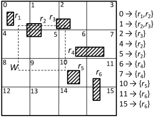
(a) grid

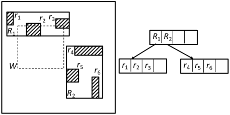
(b) R-tree

Figure 1. Examples of indexing schemes

Our goal is the design of a grid based index for non-point data which maintains the simplicity and advantages of a grid, without having its disadvantages. The niece of our index is the introduction an additional, secondary-level partitioning which divides the objects that intersect a tile into four classes ($2^{m}$ classes in an $m$-dimensional space), based on whether their MBRs start inside or before the tile in each dimension. This division helps us to avoid accessing some classes of objects during query evaluation, which reduces the query cost and at the same time avoids duplicate results, while ensuring that no results are missed. For example, in Figure 1(b), due to our second-level partitioning object $r_{2}$ will be examined and reported only by tile 0 because both the object starts in that tile and the query starts in or before that tile. We lay out the set of rules, based on which range queries using our index are evaluated. Besides, we show how our index can be used to answer distance range queries, reducing the number of expensive distance computations that alternative indexing schemes require. Finally, we show how the number of applications of the expensive refinement step can greatly be reduced.

Besides rectangular range queries, we also study the evaluation of circular range (i.e., disk) queries and, in general, queries with convex range shapes. We show how our indexing scheme reduces the number of comparisons and avoids duplicate results, also in this case. In addition, we show how for the majority of query results, the refinement step can be avoided by a simple post-filtering test on the object MBRs. Finally, we investigate the efficient evaluation of numerous range queries in batch and in parallel.

We compare our index experimentally with a state-of-the-art implementation of an in-memory R-tree from boost.org and show that it is up to several times faster, especially for large queries on large datasets. In addition, our index performs much better that the R-tree for mixed workloads (with inserts and range queries). We also show that our approach (which is directly parallelizable) scales gracefully with the number of cores (i.e., threads in a multi-core machine), making it especially suitable for shared-nothing parallel environments where tree-based spatial indexes (such as the R-tree) are hard to deploy.

In summary, this paper makes the following contributions:

• We design a novel secondary-level partitioning approach for space-partitioning indexes (such as grids).

• We show how spatial range queries can benefit from our indexing scheme, by avoiding redundant comparisons and the generation of duplicate results.

• We introduce a simple additional filter that avoids the refinement step for the great majority of the objects, rendering range queries very efficient in practice.

• We conduct an extensive experimental evaluation which demonstrates the superiority of our index in comparison to alternative methods and its scalability when evaluating multiple queries using multiple cores.

The rest of the paper is organized as follows. Section 2 provides the necessary background and discusses related work. Section 3 introduces our secondary partitioning scheme and its application in grid-based spatial indexing. Section 4 shows how spatial range query evaluation can benefit from our indexing scheme. In Section 5, we present a filtering condition that applies on the MBRs of the objects and can be used to confirm the inclusion of an object to a range query result, without the need of a refinement step. Section 6 discusses how numerous range queries that may need to be handled can be processed efficiently and in parallel. An experimental evaluation is presented in Section 7. Finally, Section 8 concludes the paper with a discussion about future work.

2. Background and Related Work

In this section, we introduce the necessary background in spatial data management (Mamoulis, 2011) and present related work to our research.

2.1. Spatial Data and Queries

Common types of spatial objects include points (defined by one value per dimension), rectangles (defined by one interval per dimension), line segments (defined by a pair of points), polygons (defined by a sequence of points), linestrings (defined by a sequence of points), etc. Three classes of spatial relationships characterize the relative position and geometry of spatial objects. Topological relationships model the relation between the geometric extents of objects (e.g., overlap, inside). Directional relationships compare the relative locations of the objects with respect to a coordinate (or cardinal) system (e.g., north/south, above/below). Last, distance relationships capture distance/proximity information between two objects (e.g., near/far).

The most frequently applied query operation on spatial data is the spatial selection or range query which retrieves the objects that satisfy a spatial relationship with a reference spatial object. Typically, the reference object is a region $W$ and the objective is to retrieve the objects that intersect $W$ or are inside $W$. In another popular range query type (especially, in location-based services), given a reference location $q$ and a distance threshold $\epsilon$, the objective is to find all objects having at most $\epsilon$ Euclidean distance from $q$. Spatial access methods are primarily designed for spatial selection queries. Other important spatial queries include nearest neighbor queries, intersection joins and distance joins.

2.2. Query Processing Principles

The potentially complex geometry of the objects renders inefficient the evaluation of spatial predicates directly on their exact representation. Hence, spatial queries are processed in two steps following a filtering-and-refinement framework. During the filtering step, the query is applied on the Minimum Bounding Rectangles (MBRs), which approximate the objects. If the MBR of an object does not qualify the query predicate, then the exact geometry does not qualify it either. The filtering step is a computationally cheap way to prune the search space, in many cases powered by spatial indexing, but it only provides candidate query results. During the refinement step, the exact representations of the candidates are tested with the query predicate to retrieve the actual results.

2.3. Spatial Partitioning and Indexing

Due to the complex nature of spatial objects, decades of research efforts have been devoted on spatial indexing; as a result, a number of Spatial Access Methods (SAMs) have been proposed (Samet, 1990, 2006). Although the majority of SAMs focus on disk-resident data, it is straightforward to also use them in main memory, which is the focus of our work. Typically, the goal of an SAM is to group closely located objects in space, into the same index blocks (traditionally, blocks are disk pages). These blocks are then organized in an index (single-level or hierarchical).

Depending on the nature of the partitioning, spatial indices can be classified into two classes (Olma et al., 2017). Indices based on space-oriented partitioning divide the space into disjoint partitions. As a result, objects whose extent overlaps with multiple partitions need to be replicated (or clipped) in each of them. A grid (Bentley and Friedman, 1979) is the simplest index based on space-oriented partitioning; the space is uniformly divided into cells (partitions), using axis-parallel lines. Hierarchical indices that fall in this category are the kd-tree (Bentley, 1975) and the quad-tree (Finkel and Bentley, 1974). Space-oriented partitioning was originally proposed and is especially suitable for indexing collections of points, because no replication issues arise. A bitmap-based index for point data was recently proposed in (Nagarkar et al., 2015). SIDI (Nguyen et al., 2016) is another spatial index for point data, which learns the characteristics of the dataset before construction and its layout is designed to fit the data well.

For non-point objects, the replication of object MBRs to multiple space-oriented partitions may negatively affect query performance. In addition, due to object replication, the same query results may be detected in multiple partitions and deduplication techniques should be applied, as discussed in the Introduction. In view of this, an alternative class of indices, based on a data-oriented partitioning, were also proposed, allowing the extents of the partitions to overlap and ensuring that their contents are disjoint (i.e., each object is assigned to exactly one partition). The R-tree (Guttman, 1984) (and its variants, e.g., the R*-tree (Beckmann et al., 1990)) is the most popular SAM in this class (and in general). The R-tree is a height-balanced tree, which generalizes the B⁺-tree in the multi-dimensional space and hierarchically groups object MBRs to blocks. Each block is also approximated by an MBR, hence the tree defines a hierarchy of MBR groups. Some R-tree variants use circles (or spheres in the 3D space) instead of MBRs, i.e., the SS-tree (White and Jain, 1996), or a combination of circles and rectangles, i.e., the SR-tree (Katayama and Satoh, 1997).

Most spatial indexing methods are designed for the efficient evaluation of spatial range queries. In brief, during the filtering step, the goal is to determine which partitions of the space intersect the query region $W$. In case of hierarchical indices such as the kd-tree, the quad-tree and the R-tree, the query is processed by recursively traversing the nodes whose MBRs intersect $W$, starting from the root. Finally, every object whose MBR overlaps with region $W$ is passed as a candidate to the refinement step where its exact geometry is compared against $W$.

Most spatial indexes have been designed to support dynamic updates. The R*-tree (Beckmann et al., 1990) differs from the original R-tree (Guttman, 1984) in its insertion algorithm, which is designed to be both efficient and to result in a high tree quality. Bulk loading methods for R-trees have also been proposed, with the most popular method being the sort-tile-recursive approach (Leutenegger et al., 1997). Naturally, updates on hierarchical indexes are more expensive, compared to updates on single-level (flat) indexes, because they may result in index reorganization. Hence, single-level indexes, such as grids are preferred over hierarchical ones in workloads with many updates (e.g., when indexing moving objects (Kalashnikov et al., 2004)).

The R-tree was originally proposed for disk-resident data with the key focus on minimizing the I/O during query processing. The CR-tree (Kim et al., 2001) is an optimized R-tree for the memory hierarchy. BLOCK (Olma et al., 2017) is a recently proposed main-memory spatial index, which uses a hierarchy of grids. At each level, a uniform grid with higher resolution compared to the level above is used. Given a range query, starting from the uppermost grid, BLOCK evaluates the query on cells that are completely contained in the query. The remaining query parts (excluding the cells that are contained in the range) are either evaluated at the cells they overlap at the current level, or they are evaluated recursively at the level below, depending on the estimated benefit.

2.4. Parallel and Distributed Data Management

Early efforts on parallel and distributed spatial query evaluation have mainly focused on spatial joins, which are more expensive than range queries and they can benefit more from parallelism. The R-tree join (RJ) algorithm (Brinkhoff et al., 1993) and PBSM (Patel and DeWitt, 1996) were parallelized in (Brinkhoff et al., 1996) and (Zhou et al., 1997; Patel and DeWitt, 2000; Ray et al., 2014b), respectively.

With the advent of Hadoop, research on spatial data management has shifted to the development of distributed spatial data management systems (Aji et al., 2013; Eldawy and Mokbel, 2015; You et al., 2015; Xie et al., 2016; Yu et al., 2019). Hadoop-GIS (Aji et al., 2013) is one of the first efforts in this direction. Spatial data in Hadoop-GIS are partitioned using a hierarchical grid, wherein high density tiles are split to smaller ones, in order to handle data skew. The nodes of the cluster share a global tile index which can be used to find the HDFS files where the contents of the tiles are stored. For query evaluation, an implicit parallelization approach is followed, which leverages MapReduce. That is, the partitioned objects are given IDs based on the tiles they reside and finding the objects in each tile can be done by a map operation. Spatial queries are implemented as MapReduce workloads. Duplicate results in spatial queries are eliminated by adding a MapReduce job at the end. In the SpatialHadoop system (Eldawy and Mokbel, 2015) data are also spatially partitioned, but different options for partitioning based on different spatial indexes are possible (i.e., grid based, R-tree based, quadtree based, etc.) Different spatial datasets could be partitioned by a different approach. A global index for each dataset is stored at a Master node, indexing for each HDFS file block the MBR of its contents. In addition, a local index is built at each physical partition and used by map tasks.

Spark-based implementations of spatial data management systems (You et al., 2015; Xie et al., 2016; Yu et al., 2019) apply similar partitioning approaches. The main difference to Hadoop-based implementations is that data, indexes, and intermediate results are shared in the memories of all nodes in the cluster as resilient distributed datasets (RDDs) and can be made persistent on disk. Unlike SpatialSpark (You et al., 2015) and GeoSpark (Yu et al., 2019) which are built on top of Spark, Simba (Xie et al., 2016) has its own native query engine and query optimizer, however, Simba does not support non-point geometries. Pandey et al. (Pandey et al., 2018) conduct a comparison between in-memory spatial analytics systems and find that they scale well in general, although each one has its own limitations. Similar conclusions are drawn in another study (Alam et al., 2018).

We observe that distributed spatial data management systems focus more on data partitioning and less on minimizing the cost of query evaluation at each partition. In other words, emphasis is given on scaling out (i.e., making the cost anti-proportional to the number of nodes), rather than on per-node scalability (i.e., reducing the computational cost per node) and multi-core parallelism. For example, a typical range query throughput rate reported by the tested systems in (Pandey et al., 2018; Alam et al., 2018) is a few hundred queries per minute, whereas for the same scale of data an in-memory R-tree can handle on a single machine (without parallelism) tens of thousands of queries per minute (according to our tests in Section 7).

3. Two-level Spatial Partitioning

We consider the classic approach of approximating spatial objects by their minimum bounding rectangles (MBRs). By imposing a $N\times M$ regular grid over the space, we can divide it into $N\cdot M$ disjoint tiles. Determining $N$ and $M$ is not a subject of this section; we will discuss/study this issue in Section 7. Each tile divides a spatial partition. An object $o$ is assigned to a tile $T$ if $MBR(o)$ and $T$ intersect (i.e., they have at least one common point); in this case, $o$ is assigned to tile $T$. Since $MBR(o)$ can intersect with multiple tiles, $o$ can be assigned to more than one tiles. We target applications where the object extents are relatively small compared to the map (and to the extent of a tile); hence object replication is expected to be low.

For example, Figure 2 shows a grid and a spatial object $o_{1}$, whose MBR intersects tiles $T_{a}$ and $T_{b}$; $o_{1}$ is assigned to both tiles. For each tile $T$, we keep a list of (MBR, object-id) pairs that are assigned to $T$. For example, the MBR and id of $o_{1}$ in Figure 2 appears in the list of $T_{a}$ and $T_{b}$. This means that while the MBRs and ids of the objects can be replicated to multiple tiles, the actual geometry of an object is stored only once in a separate data structure (e.g., an array or a hash-map) in order to be retrieved fast, given the object’s id. Since the spatial distribution of objects may not be uniform, there could be empty tiles. If the number of empty tiles is significantly large compared to the total number of tiles, we can use a hash-map to assign each non-empty tile to the set of rectangles in it. The above storage scheme is quite effective for main-memory data because it supports queries and updates quite fast, while it is straightforward to parallelize popular spatial queries and operations.

3.1. Evaluating queries over a simple grid

We now discuss in more detail how this simple indexing scheme can be used to evaluate rectangular range queries and expose its limitations. We first introduce some notation that will also be useful when we discuss our solution.

Recall that each MBR $r$ can be represented by an interval of values at each dimension. Let $r[i]=[r[i][0],r[i][1]]$ be the projection of rectangle $r$ on the $i$-th axis. For example, in the 2D space, $r[0][1]$ denotes the upper bound of rectangle $r$ on dimension $0$ (i.e., the $x$-axis). Similarly, we use $T[i]=[T[i][0],T[i][1]]$ to denote the projection of a tile $T$ to the $i$-th dimension. Given a tile $T$ and a dimension $i$, we use $prev(T,i)$ to denote the tile $T^{\prime}$ which is right before $T$ in dimension $i$ and has exactly the same projection as $T$ in the other dimension(s). For example, in Figure 2, $T_{b}=prev(T_{a},0)$. $prev(T,i)$ is not defined for tiles $T$ which are in the first column (for $i=0$) or row (for $i=1$) of the grid.

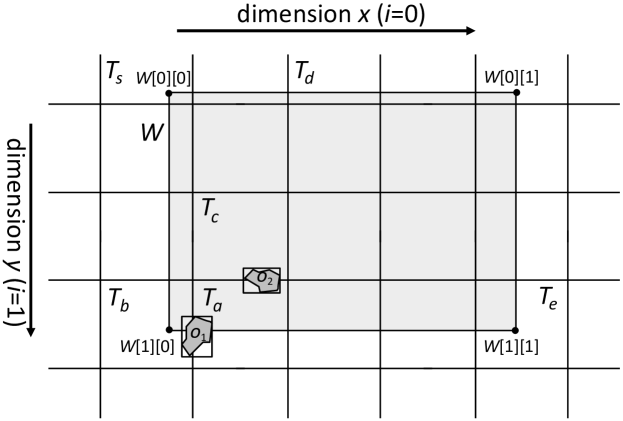
Figure 2. Example of tiling and query evaluation

Given a range query window $W$, a tile that does not intersect $W$ does not contribute any results to the query. Specifically, the only tiles $T$ that may contain query results are those for which $T[i][1]\geq W[i][0]$ and $T[i][0]\leq W[i][1]$ at every dimension $i$ and can easily be enumerated after finding the tiles $T_{s}$ and $T_{e}$, which contain $W[0][0]$ and $W[1][1]$, respectively. Figure 2 illustrates a window query $W$ in lightgrey color and its four corner points $W[0][0]$, $W[0][1]$, $W[1][0]$, $W[1][1]$. The tiles which are relevant to $W$ are between (in both dimensions) the two tiles $T_{s}$ and $T_{e}$.

For each tile which is totally covered by the query range in at least one dimension (e.g., $T_{a}$ in dimension $0$), we know that the objects in it certainly intersect $W$ in that dimension. For a tile $T$ that partially overlaps with $W$ in both dimensions (e.g., $T_{b}$), we need to iterate through its objects list to verify their intersection with $W$. We first check whether the MBR of the object intersects $W$ and then we might have to verify with the exact geometry of the object at a refinement step.

An important issue is that neighboring tiles may intersect $W$ and also contain the same object $o$. In this case, $o$ will be reported more than once, so we need an approach for handling these duplicates. For example, in Figure 2, object $o_{1}$ could be reported both by $T_{a}$ and by $T_{b}$. A solution to this problem is to report an object $o$ only at the tile which is before all tiles (in both dimensions) where $o$ is found to intersect $W$. For example, in Figure 2, $o_{1}$ is reported by $T_{b}$ only, which is before $T_{a}$. An easy approach to perform this test is to compute the intersection between the query window and the rectangle and report the result only if a reference point of the intersection (e.g., the smallest value in all dimensions) is included in the tile (Dittrich and Seeger, 2000). While this solution prevents reporting duplicates, it requires extra comparisons and it is unclear how to apply it for non-rectangular range queries. An alternative and more general approach is to add the results from all tiles in a hash table, which would prevent the same rectangle from being added multiple times.

3.2. A Second Level of Partitioning

We now present our proposal for improving this basic spatial indexing approach by introducing a second level of partitioning to the contents of each tile. Our approach avoids the generation of duplicate results overall and, hence, it does not require any duplicate elimination. We propose that the set of MBRs in each tile is further divided into four classes $A$, $B$, $C$, and $D$ (which are physically stored separately in memory). Specifically, consider a rectangle $r$ which is assigned to (i.e., intersects) tile $T$.

• $r$ belongs to class $A$, if for every dimension $i$, the begin value $r[i][0]$ of $r$ falls into projection $T[i]$, i.e., if $T[i][0]\leq r[i][0]$.

• $r$ belongs to class $B$ if its $x$-projection $r[0]$ begins inside $T[0]$, but its $y$-projection $r[1]$ begins before $T[1]$, i.e., if $T[0][0]\leq r[0][0]$ and $T[1][0]>r[1][0]$.

• $r$ belongs to class $C$ if its $x$-projection $r[0]$ begins before $T[0]$, but its $y$-projection $r[1]$ begins inside $T[1]$, i.e., if $T[0][0]>r[0][0]$ and $T[1][0]\leq r[1][0]$.

• $r$ belongs to class $D$ if both its $x$- and $y$-projections begin before $T$, i.e., if $T[0][0]>r[0][0]$ and $T[1][0]>r[1][0]$.

We can refer to each class by two bits, one for each dimension. The bit in each dimension indicates whether the rectangle starts before the tile in that dimension. Hence, class $A$ can also be referred to as class $00$ because a rectangle in class $A$ of a tile $T$ does not start before $T$ in both dimensions. Similarly, classes $B$, $C$, and $D$ can be denoted by $01$, $10$, and $11$, respectively. This notation can generalized to an arbitrary number of dimensions $m$, where there are $2^{m}$ classes of bounding boxes in each multidimensional tile and $m$ bits are used to denote each class.

Figure 3 illustrates examples of rectangles in a tile $T$ that belong to the four different classes. During data partitioning, for each tile $T$ a rectangle $r$ is assigned to, we identify its class and, hence, for each tile, we have four different rectangle divisions (which are stored separately). Note that a rectangle can belong to class $A$ of just one tile, while it can belong to other classes (in other tiles) an arbitrary number of times.

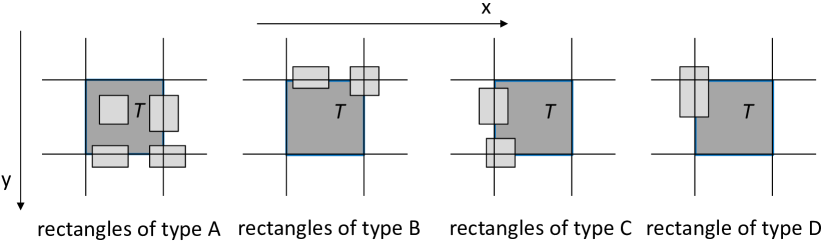
Figure 3. The 4 classes of rectangles inside a tile $T$.

4. Range Query Evaluation

In this section, we show how the divisions can be used to evaluate spatial range queries efficiently and at the same avoid generating and testing duplicate query results. For simplicity, we first consider rectangular range queries where the query range is a rectangle (window) $W$ and the objective is to find the objects which spatially intersect $W$. The cases of other query shapes will be discussed later on. For now, we focus on the filtering step of the query, i.e., the objective is to find the object MBRs which intersect $W$. The refinement step will be discussed in Section 5.

Recall that the tiles which are relevant to $W$ are between the two tiles that contain $W[0][0]$ and $W[1][1]$ in both dimensions. We lay out a set of rules that can be used to determine which rectangles in each of these tiles are query results and what are the necessary comparisons for determining whether a rectangle is a result. Finally, these rules can help us to avoid generating and eliminating duplicate query results, without any comparisons, bookkeeping, or synchronization in the processing at different tiles. In summary, the goal of our method is twofold: (i) eliminate any dependencies between processing at different tiles and (ii) minimize the cost of processing at each tile, by avoiding redundant comparisons and duplicate result checks.

4.1. Selecting relevant classes

Recall that in order for two rectangles to intersect (in our case $W$ and a candidate query result), they should intersect in all dimensions. In order words, if a rectangle $r$ does not intersect $W$ in one dimension (i.e., in a dimension $i$, we either have $r[i][1]<W[i][0]$ or $W[i][1]<r[i][0]$), then $r$ is not a query result. We now present a lemma which can help us to determine classes of rectangles in a tile that should not be considered in a query, otherwise they would produce duplicate results.

Lemma 0 (Filtering).

If $W$ intersects tile $T$ and starts before $T$ in dimension $i$, then:

• in the classes having $1$ in dimension $i$, all rectangles that intersect $W$ are guaranteed to intersect $W$ also in the previous tile $prev(T,i)$ hence they can be safely disregarded;

• if also $W$ starts before $T$ in dimension $j\neq i$, then all objects in the class having $1$ in dimension $j$ are guaranteed to intersect $W$ also in the previous tile $prev(T,j)$ hence they can be safely disregarded.

To understand the first point of the lemma, consider again Figure 2 and tile $T_{a}$; $W$ starts before $T_{a}$ in dimension $0$. All rectangles of $T_{a}$ in classes $C=10$ and $D=11$ can be ignored by tile $T_{a}$ when processing query $W$ because these rectangles are guaranteed to also intersect the previous tile $T_{b}=prev(T_{a},0)$ in dimension $0$ and they can be processed there. Hence, $o_{1}$ (which belongs to class $C=10$) is not examined at all by tile $T_{a}$.

To understand the second point of the lemma, consider object $o_{2}$ in Figure 2. Note that $W$ also starts before $T_{a}$ in dimension $1$. This guarantees that all objects in class $B=01$ of tile $T_{a}$ which intersect $W$ can be reported at tile $T_{c}=prev(T_{a},1)$, so $T_{a}$ can safely ignore all rectangles in class $B=01$.

4.2. Reduction of comparisons

We now turn our attention to minimizing the comparisons needed for rectangle classes that have to be checked (i.e., those not eliminated by Lemma 1). If a tile $T$ is covered by the window $W$ in a dimension $i$, then we do not have to perform intersection tests in that dimension. Let us go back to the example of Figure 2. Recall that only rectangles in class $A=00$ of tile $T_{a}$ need to be checked against window $W$, because the other classes have been filtered out by Lemma 1. For all these rectangles, we only have to conduct an intersection test with $W$ in dimension $1$, since $T_{a}$ is totally covered by $W$ in dimension $0$. For the dimension(s) where the tile is not covered by $W$, the following lemmas can be used to further reduce the necessary comparisons.

Lemma 0 (Comparisons Reduction 1).

If $W$ ends in tile $T$ and starts before $T$ in dimension $i$, then for a rectangle $r\in T$, $r$ intersects $W$ in dimension $i$ iff $r[i][0]\leq W[i][1]$.

For example, in tile $T_{a}$, we only have to test intersection in dimension $1$ for rectangles $r$ in class $A=00$, as already explained. The intersection test can be reduced to a simple comparison, i.e., if $r[1][0]\leq W[1][1]$ then $r$ intersects $W$. Symmetrically, we can show:

Lemma 0 (Comparisons Reduction 2).

If $W$ starts in tile $T$ and ends after $T$ in dimension $i$, then for a rectangle $r\in T$, $r$ intersects $W$ in dimension $i$ iff $r[i][1]\geq W[i][0]$.

For example, consider tile $T_{d}$ in Figure 2. Due to Lemma 1, we can eliminate from consideration rectangle classes $C=10$ and $D=11$ in $T_{d}$, while for the rectangles in classes $A=00$ and $B=01$, the rectangles are guaranteed to intersect $W$ in dimension $0$. Hence, we only have to find the rectangles $r$ in classes $A$ and $B$, for which $r[1][1]\geq W[1][0]$.

Example. A detailed example of the tasks executed by each tile in a window query $W$ is illustrated in Figure 4. Tile $T_{1}$ processes all four classes of its rectangles. For each rectangle, just one comparison is needed per dimension due to Lemma 3. Tiles $T_{2}$–$T_{5}$ process only classes $A=00$ and $B=01$ due to Lemma 1. In $T_{2}$–$T_{4}$, the intersection test at dimension $0$ is skipped. In addition, for each rectangle, only one comparison is necessary (Lemma 3). Tile $T_{5}$ applies one comparison in each dimension using the start and end points in dimensions $0$ and $1$, respectively (Lemmas 2 and 3). For tile $T_{6}$ only rectangle classes $A=00$ and $C=10$ need to be processed and Lemma 3 can be used to reduce the comparisons for dimension $0$, while there is no need for comparisons in dimension $1$, as $W$ covers the tile in this dimension. For tiles $T_{7}$–$T_{10}$, only rectangle classes $A=00$ are accessed. For tiles $T_{7}$–$T_{9}$, no comparisons at all are required, whereas for tile $T_{10}$, one comparison for dimension $0$ should be performed (Lemma 2). Tiles $T_{11}$–$T_{15}$ are processed as tiles $T_{6}$–$T_{10}$ (respectively). Tile $T_{16}$ processes classes $A=00$ and $C=10$ only and two comparisons for each rectangle are required. Tiles $T_{17}$–$T_{20}$ process only class $A=00$. In Tiles $T_{17}$–$T_{19}$, one comparison per rectangle is required (Lemma 2), while Tile $T_{20}$ requires two comparisons per rectangle.

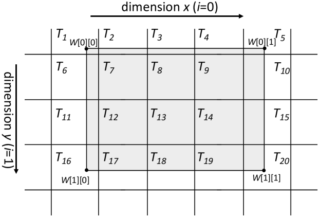
Figure 4. Processing a range query at each tile

4.3. Overall approach

Given a range query $W$, we first identify the range of tiles that intersect $W$ (i.e., the first and the last tile in each dimension) by simple algebraic operations (i.e., by dividing the endpoints of $W$ in each dimension by the number of space divisions in that dimension). We then pass the control to each tile $T$, which accesses the relevant classes of rectangles and perform the necessary computations for the rectangles in them. For each qualifying rectangle a refinement step is performed (after accessing the corresponding object’s geometry). The results produced at each tile are eventually merged.

4.4. Disk queries

We now discuss the evaluation of disk range queries, where the objective is to find all objects which overlap a disk $D$ of radius $\epsilon$ centered at a given point $q$. This query is equivalent to a distance range query of the following form: “find all objects having distance at most $\epsilon$ from location $q$” and it is very popular in location based services applications.

To evaluate a disk query on our two-level partitioned dataset, we apply a similar method, as for the rectangular window queries that we have seen already; we first find the tiles that intersect with the disk and then the objects in them that satisfy the query predicate. If we approximate the disk $D$ by $MBR(D)$, we can easily identify the tiles that potentially intersect the disk by simple algebraic computations, as in window queries. For each such tile, its minimum distance to $q$ is computed and, if the distance is found at most $\epsilon$, the tile is confirmed to intersect the disk.

We turn our attention to computing results in a tile and to duplicate avoidance. Since a rectangle can be assigned to multiple tiles, the objective is to examine only the MBR classes in each tile which are necessary to ensure that (i) no result is missed and (ii) no duplicate results are reported. In other words, all rectangles that intersect the disk should be reported exactly once. For this, we follow a similar approach as for the case of rectangular queries. For each tile $T$, where $T$ is within distance $\epsilon$ from $q$, we check whether $prev(T,i)$ in each dimension $i$ is also within distance $\epsilon$ from $q$, i.e., whether $prev(T,i)$ is in the set of tiles $S$ that may include results. If yes, then we disregard the corresponding class of rectangles in $T$. Hence, if $prev(T,0)\in S$, then class $B=01$ is disregarded, whereas if $prev(T,1)\in S$, then class $C=10$ is disregarded. If $prev(T,0)\in S$ and $prev(T,1)\in S$, then all classes $B,C,D$ are disregarded.

Figure 5 shows an example of a disk query centered at q. The tiles which intersect the disk are shown by different patterns depending on the classes of rectangles in them that have to be checked. For example, in tile $T_{5}$ all four classes will be examined (we call $T_{5}$ an $ABCD$ tile, in the context of the disk query). Note that for the majority of tiles which intersect the disk range, we only have to examine rectangles in class $A=00$.

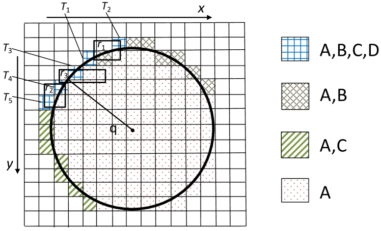
Figure 5. Example of disk query evaluation

A subtle point here is that if we simply examine all rectangles in the classes that correspond to each tile, we may end up examining duplicates. For example, consider rectangle $r_{1}$, which will be examined in both tiles $T_{1}$ (in class $B$) and $T_{2}$ (in class $C$). To avoid such duplicates, for each rectangle in an $ABCD$ tile $T$, if the tile is closer to $q$ in the $y$-dimension compared to the $x$-dimension, we ignore rectangles $r$ in classes $C$ and $D$, for which $r[1][1]>T[1][1]$ (these will be handled in another tile). For example, in tile $T_{2}$, we ignore rectangles in classes $C$ or $D$, which “overflow” to the tile below $T_{2}$ (such as $r_{1}$). If the tile is closer to $q$ in the $x$-dimension compared to the $y$-dimension, we ignore rectangles $r$ in classes $B$ and $D$, for which $r[0][1]>T[0][1]$. For example, in tile $T_{5}$, we ignore rectangles in classes $B$ or $D$, which “overflow” to the tile on the right of $T_{5}$ (such as $r_{2}$). Finally, for a single tile, which has (almost) the same distance to $q$ in both dimensions, we consider all rectangles, regardless whether they “overflow” or not to the next tiles. For example, for tile $T_{3}$ we consider all rectangle classes, i.e., rectangle $r_{3}$ will be examined in $T_{3}$ and not in $T_{4}$.

Before examining the rectangles in the tiles in $S$ (only the relevant classes), we can compute the maximum distance between the tile and $q$, and if this distance is found to be at most $\epsilon$, then the tile is marked as covered by the disk. For tiles which are covered by the disk, we do not have to verify any distances between the objects assigned to them and $q$, as these distances are guaranteed to have distance at most $\epsilon$ from $q$ (i.e., they are definite results). Again, at each row, the set of tiles which are covered by the disk are continuous, meaning that we only have to check the tiles in both directions starting from the tile which includes $q$ in dimension $x$ until we find the first one that violates the maximum distance condition.

Finally, the method described above for disk queries can be generalized for any query whose range is a convex polygon. We first find the set of tiles $S$ which intersect the query range. Then, for each tile $T\in S$, we determine which classes of objects need to be examined (i.e., exclude classes that would produce duplicates). For each tile which is totally covered by the query region, we just report its contents in the relevant classes as results and for the remaining tiles we conduct an intersection test for each rectangle before determining whether it is a result.

5. Refinement Avoidance

We now discuss the evaluation of the refinement step of range queries on our two-level partitioning index. We begin by a general and important lemma, which applies independently to our index and greatly reduces the number of objects for which the refinement step needs to be applied, especially for query ranges which are relatively large.

Lemma 0 (Refinement Step Avoidance).

Given a candidate object whose MBR $r$ intersects the query range, if at least one side of $r$ is inside the query range, then the object is guaranteed to intersect the range and no refinement step is necessary.

The lemma is trivial to prove, based on the definition of MBR. Recall that the MBR of an object is defined by the minimum and maximum values of the object in every dimension. Hence, at each side of the MBR, there is at least one point which is part of the object’s geometry. If one side of the MBR is inside the query range, then there should be at least one point of the object inside the query range, i.e., the object and the range intersect. The lemma generalizes to more than two dimensions. In a $d$-dimensional space, we test if at least one of the $(d-1)$-dimensional faces of the minimum hypercube that bounds the object is inside the query range.

For different range shapes, we can define specialized MBR side coverage tests. Consider a rectangular query range $W$ and an object MBR $r$ that intersects $W$. To apply a refinement avoidance test, we should verify if $W$ covers $r$ in at least one dimension. If this is true, given that $r$ intersects $W$, one of the cases shown in Figure 6(a) should happen. Either one side of $r$ is inside the window $W$ and Lemma 1 applies (see $r_{a}$ in Figure 6(a)) or $r$ splits $W$ along the coverage axis (see $r_{b}$ in Figure 6(a)). In both cases, whatever the geometry of the object is the object definitely intersects $W$. For a disk query range $D$, we can check whether there are at least two corners of $r$ whose distances to the disk center are smaller than or equal to the disk radius. For example, in Figure 6(b), rectangle $r_{1}$ has at least two corners in the disk range, which means that at least one side of the rectangle is in the range and Lemma 1 applies. On the other hand, only one corner of $r_{2}$ is inside the disk, hence the refinement step for the corresponding object cannot be avoided.

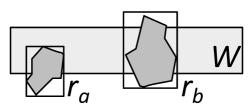
(a) window query

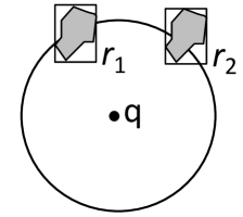
(b) disk query

Figure 6. Refinement step avoidance

Let us now turn our focus to our index and see how we can take advantage of Lemma 1 to apply the refinement avoidance test and minimize the necessary comparisons. The main idea is to study the refinement avoidance test at the tile level, in order to limit the comparisons required for each class of objects in the tiles.

Specifically, for each $T$ that intersects a query range $W$ and for each dimension $i$, we consider two cases: (i) $W$ starts before $T$ in dimension $i$, i.e., $W[i][0]<T[i][0]$ and (ii) $W[i][0]\geq T[i][0]$. In the first case, due to Lemma 1, only classes of rectangles that start inside $T$ in dimension $i$ are considered, which means for each rectangle $r\in T$ which is found to intersect $W$, we already know that $W[i][0]<r[i][0]$. Hence, we only have to test if $r[i][1]\leq W[i][1]$ to confirm that $r$ is covered by $W$ in dimension $i$ and that the refinement step for $r$ is not necessary. On the contrary, for the case where $W[i][0]\geq T[i][0]$, we should apply the complete refinement avoidance test in dimension $i$ (i.e., $W[i][0]\leq r[i][0]$ and $r[i][1]\leq W[i][1]$) for each $r\in T$ which is found to intersect $W$.

As an example, consider again the query in Figure 4. For each rectangle in tile $T_{1}$ found to intersect $W$, we should apply the complete coverage test in each of the two dimensions, before applying the refinement step. For each rectangle $r$ in tiles $T_{2}$–$T_{5}$ and for dimension $0$ we only have to test if $r[0][1]\leq W[0][1]$, since these rectangles are in classes $A$ and $B$ and they start inside the tile in dimension $0$. Similarly, for each rectangle $r$ in tiles $T_{6}$, $T_{11}$, and $T_{16}$ and for dimension $1$ we only have to test if $r[1][1]\leq W[1][1]$, since these rectangles are in classes $A$ and $C$ and they start inside the tile in dimension $1$. For all remaining tiles, if $r[0][1]\leq W[0][1]$ or $r[1][1]\leq W[1][1]$ holds, $r$ is guaranteed to be a true result and no refinement is necessary.

6. Batch Query Processing

In the previous sections, we presented how our two-level index handles single query requests. Real systems however receive and need to evaluate a large number of concurrent queries. Under this, we next discuss how to efficiently process batches of spatial range queries. Although our focus is primarily in a single-threaded processing environment, parallel query processing in modern multi-core hardware can also benefit from the ideas discussed in this section. To this end, our experimental analysis includes both single-threaded and multi-threaded experiments.

Naturally, a straightforward approach for processing a workload of concurrent spatial range queries is to evaluate every query independently, directly applying the ideas discussed in the previous sections. In a parallel processing environment, we can easily adopt this approach by assigning the queries to the available threads in a round robin fashion. We call this simple approach $\mathsf{queries}\mbox{-}\mathsf{based}$. Its main shortcoming is that it is cache agnostic; as every issued query $q$ typically overlaps multiple tiles of the grid, the computation of $q$ requires accessing data structures in different parts of the main memory, i.e., the memory access pattern is prone to cache misses. The problem is present also in parallel query processing, as every thread goes through multiple rounds of “content switching”.

To address this shortcoming of $\mathsf{queries}\mbox{-}\mathsf{based}$, we design a cache-conscious two-step approach. Given a large batch of queries $Q$, for each tile, accumulate the subtasks of all queries in $Q$ that intersect the tile. Each subtask corresponds to accessing and processing (the relevant to the query) classes of rectangles in the tile. Then, in a second step, we initiate one process at each tile, which evaluates the corresponding subtasks. Essentially, query processing is no longer driven by the queries, but from the grid tiles and therefore, we call this approach $\mathsf{tiles}\mbox{-}\mathsf{based}$. This method is favored by parallel processing, since each thread (corresponding to a tile) can benefit from the processor’s cache while processing the subtasks assigned to it. As we demonstrate in Section 7 the $\mathsf{tiles}\mbox{-}\mathsf{based}$ approach scales better with the number of parallel threads compared to $\mathsf{queries}\mbox{-}\mathsf{based}$.

7. Experimental Evaluation

In this section we present our experimental analysis. We first describe our setup and then our experiments, which investigate the construction and update costs of our two-level index as well as its efficiency and scalability in spatial range query evaluation.

7.1. Setup

Our analysis was conducted on a machine with 384 GBs of RAM and a dual Intel(R) Xeon(R) CPU E5-2630 v4 clocked at 2.20GHz running CentOS Linux 7.6.1810. All methods were implemented in C++, compiled using gcc (v4.8.5) with flags -O3, -mavx and -march=native. For our parallel processing tests, we used OpenMP and activated hyper-threading, allowing us to run up to 40 threads.

Table 1. Datasets used in the experiments

dataset	type	card.	avg. $x$-extent	avg. $y$-extent
AREAWATER	polygons	$2.3$M	$0.00000723$	$0.00002296$
LINEARWATER	linestrings	$5.8$M	$0.00002224$	$0.00007319$
ROADS	linestrings	$20$M	$0.00001254$	$0.00004067$
EDGES	polygons	$70$M	$0.00000610$	$0.00001982$

Datasets. We experimented with four of the publicly available Tiger 2015 datasets (Eldawy and Mokbel, 2015). The input objects were normalized so that the coordinates in each dimension take values inside $[0,1]$. Table 1 provides statistics about the datasets we used. The datasets contain from 2.3M to 70M objects, either polygons or linestrings. The last two columns of the table are the relative (over the entire space) average length for every object’s MBR at each axis.

Methods. We designed two variants of our two-level indexing approach (presented in Section 3.2). In the first one termed $\mathsf{2\mbox{-}level}$, each tile of the grid stores the (MBR, id) pairs of the indexed objects in four tables (one for each of the $A$, $B$, $C$, $D$ classes), such that there is no particular order of the contents of each table (i.e., as in a heap file). This organization supports insertions efficiently as the MBRs of new objects are simply appended to the tables of the tiles. In the second variant, termed $\mathsf{2\mbox{-}level^{+}}$, the MBRs of each class are also stored in four decomposed tables, following the Decomposition Storage Model (DSM) (Copeland and Khoshafian, 1985), adopted by column-oriented database systems (e.g., (Stonebraker et al., 2005)). Specifically, each rectangle $r$ with id $i$ is decomposed to four tuples, i.e., $\langle r[0][0],i\rangle$, $\langle r[0][1],i\rangle$, $\langle r[1][0],i\rangle$, $\langle r[1][1],i\rangle$ and each tuple is stored in a dedicated table. The tables are sorted by their first column and used to evaluate fast queries on tiles, where just one endpoint of each MBR needs to be compared (see Lemmas 2 and 3). In this case, $\mathsf{2\mbox{-}level^{+}}$ takes advantage of the sorted decomposed tables to reduce the information that has to be accessed and the number of comparisons. For example, in tile $T_{2}$ of Figure 4, we only have to access the decomposed tables of classes $A$ and $B$ with $\langle r[1][1],i\rangle$ tuples to test whether $r[1][1]\geq W[1][0]$ for each rectangle there. Since these tuples are sorted, we perform binary search to find the first qualifying tuple in each table and then scan the tables forward from thereon. $\mathsf{2\mbox{-}level^{+}}$ processes window queries very fast, but it is suited mostly for static data.

We also considered three competitors to our indexing scheme. The $\mathsf{1\mbox{-}level}$ scheme, discussed in Section 3.1, indexes the MBRs of the input objects using a simple uniform grid; MBRs that span multiple tiles are replicated accordingly, but our proposal for a second level of indexing (i.e., Section 3.2) is not applied. When processing window queries, $\mathsf{1\mbox{-}level}$ performs duplicate elimination using the reference point approach (Dittrich and Seeger, 2000). The second competitor is an in-memory STR-bulkloaded R-Tree (Leutenegger et al., 1997) taken from the Boost library (boost.org), which has a fanout of 16 for both inner and leaf nodes. This configuration is reported to perform the best (we also confirmed this by testing). The third competitor is BLOCK; the implementation was kindly provided by the authors of (Olma et al., 2017). After testing this approach we found it to be orders of magnitude slower that the R-tree (BLOCK takes seconds to evaluate range queries on our data), which can be attributed to the fact that BLOCK is implemented for 3D objects. Therefore, we decided to exclude BLOCK from the reported measurements.

Tests and parameters. To assess the effectiveness of the tested indices, we compared their space requirements, their building and update costs and their query performance. For the partitioning-based schemes, i.e., $\mathsf{1\mbox{-}level}$, $\mathsf{2\mbox{-}level}$ and $\mathsf{2\mbox{-}level^{+}}$, we investigated the best granularity for their grid by varying the number of partitions (i.e., divisions) per dimension. By default, we use 2000 per dimension, resulting in a 2000$\times$2000 grid. We experimented with both window and disk queries by varying their relative extent over the entire data space. We considered both cases of single and batch query processing, measuring the average execution time per query and the total execution time, respectively. Especially, for parallel batch query processing, we also experimented with the number of available threads. At each experimental instance, we averaged the cost of 10000 queries applied on non-empty areas of the map (i.e., the queries always return results). By default the areas of the queries are $0.1$% of the area of the map.

7.2. Filtering Vs Refinement

filtering    avoidance    refinement   

AREAWATER	LINEARWATER	ROADS	EDGES
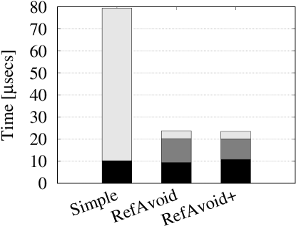
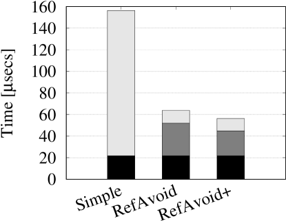
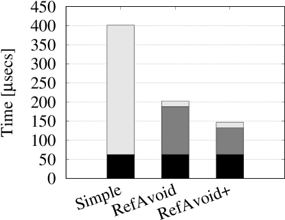
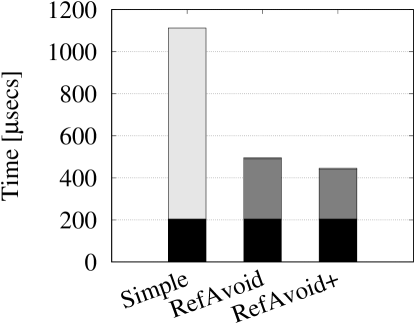
Window queries
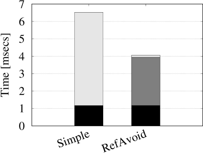
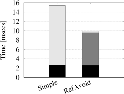
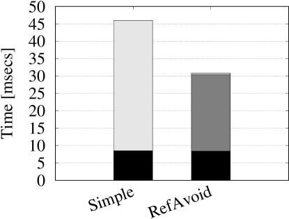
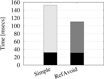
Disk queries

Figure 7. Time breakdown: $\mathsf{2\mbox{-}level}$ indexing with 2000 partitions per dimension, 10000 queries of 0.1% extent ratio

We first justify our decision to focus on and optimize the filtering step of range query evaluation, which in fact has been the primary target of previous works as well. We used our $\mathsf{2\mbox{-}level}$ index to execute both the filtering and refinement steps. We consider three variants of query evaluation depending on the way refinement is performed (see Section 5); filtering is identical in all three variants. More specifically, under Simple, all candidates identified by the filtering step are passed to the refinement step; RefAvoid employs Lemma 1 as an extra pre-refinement filter to significantly reduce the number of candidates to be refined; last, $\mathsf{RefAvoid^{+}}$ enhances RefAvoid by reducing the number of comparisons required for testing Lemma 1 in window queries, as discussed at the end of Section 5.

Figure 7 illustrates the breakdown of the average execution time for both window and disk queries; note that for disk queries $\mathsf{RefAvoid^{+}}$ is not applicable. We make two important observations. First, the figure clearly shows the effectiveness of the refinement avoidance technique discussed in Section 5. Both RefAvoid and $\mathsf{RefAvoid^{+}}$ significantly reduce the number of candidates to be refined by over 90% and so, their refinement step is always lower than that of Simple. To achieve this however, they apply a refinement avoidance test on the MBRs; the cost of this is higher in case of disk queries because it requires expensive distance computations between the disk center and the corners of object MBRs. The second observation is that, when our refinement avoidance technique is used, the bottleneck of the query is in the filtering step. Hence, in the subsequent experiments, we focus on the filtering step of spatial query processing.

7.3. Indexing and Tuning

AREAWATER	LINEARWATER	ROADS	EDGES
partitions per dimension [$\times 1000$]	partitions per dimension [$\times 1000$]	partitions per dimension [$\times 1000$]	partitions per dimension [$\times 1000$]
partitions per dimension [$\times 1000$]	partitions per dimension [$\times 1000$]	partitions per dimension [$\times 1000$]	partitions per dimension [$\times 1000$]
partitions per dimension [$\times 1000$]	partitions per dimension [$\times 1000$]	partitions per dimension [$\times 1000$]	partitions per dimension [$\times 1000$]

Figure 8. Indexing and tuning: varying the granularity of the grid, 10000 window queries of 0.1% relative extent

We next investigate the building cost and the tuning of our two-level index. Figure 8 reports the indexing time for both $\mathsf{2\mbox{-}level}$ and $\mathsf{2\mbox{-}level^{+}}$ variants and the size of each index, while varying the granularity of the underlying grid partitioning. For reference and completeness purposes, we include the $\mathsf{1\mbox{-}level}$ competitor which also uses a uniform grid to partition the input space. As the goal of the index is to efficiently answer spatial range queries, we additionally report the average query time in order to determine the best grid granularity.

Naturally, the indexing cost for all three indices grows while increasing the granularity of the grid. As expected, both $\mathsf{1\mbox{-}level}$ and $\mathsf{2\mbox{-}level}$ have the same space requirements. Regardless of employing the second level of partitioning or not, both indices store exactly the same number of object MBRs (originals and replicas); the difference is that inside each tile, $\mathsf{2\mbox{-}level}$ divides the rectangles in four classes and stores them in dedicated structures while $\mathsf{1\mbox{-}level}$ stores all rectangles together. In terms of the indexing time, $\mathsf{2\mbox{-}level}$ is slightly more expensive than $\mathsf{1\mbox{-}level}$, as it needs to first determine the class for each rectangle and then store it accordingly. On the other hand, the indexing cost of $\mathsf{2\mbox{-}level^{+}}$ is higher than both $\mathsf{1\mbox{-}level}$ and $\mathsf{2\mbox{-}level}$ indices. Remember that $\mathsf{2\mbox{-}level^{+}}$ essentially stores a second copy of the rectangles inside every tile, after decomposing their coordinate information. As a result, the size of $\mathsf{2\mbox{-}level^{+}}$ is 2.4x larger; its building time is also higher due to the cost of computing, sorting and storing the decomposed replicas of the rectangles. The sizes of the packed R-trees (not shown) are about the same as the sizes of the corresponding $\mathsf{1\mbox{-}level}$ (and $\mathsf{2\mbox{-}level}$) indices when 2000 partitions per dimension are used, indicating that the replication ratio of our indexes is very low. In addition, the bulk loading costs of the R-trees are 0.53s, 1.4s, 5.2s, and 19.5s for the four datasets, respectively, i.e., about 20% lower compared to the construction cost of $\mathsf{2\mbox{-}level^{+}}$.

Let us now study the efficiency of each index. The key observation is that employing the second level of indexing significantly enhances query processing; $\mathsf{2\mbox{-}level}$ and $\mathsf{2\mbox{-}level^{+}}$ always outperform $\mathsf{1\mbox{-}level}$. Due to lack of space, Figure 8 reports only on window queries, but the same trend applies for disk queries. The fastest index is $\mathsf{2\mbox{-}level^{+}}$ as it trades the extra used space for better query performance; nevertheless, $\mathsf{2\mbox{-}level}$ is also significantly faster than $\mathsf{1\mbox{-}level}$. The last observation is that all three indices perform at their best when the underlying grid defines approximately 2000 partitions per dimension. Under this configuration, the number of tiles is not excessive and the indices do not have a large overhead in accessing and managing tiles; at the same time the rectangles are small enough compared to the tile extent (see Table 1), in order not to incur excessive replication. For the rest of our analysis, $\mathsf{1\mbox{-}level}$, $\mathsf{2\mbox{-}level}$ and $\mathsf{2\mbox{-}level^{+}}$ all use a 2000$\times$2000 uniform grid.

7.4. Cost of Updates

In order to confirm the superiority of our proposed indexing scheme in updates compared to the R-tree, we conducted an experiment, where for all datasets, we first constructed the index by loading 90% of the data in batch and then we measured the cost of incrementally inserting the last 10% of the data. Table 2 compares the total update costs of the R-tree, $\mathsf{1\mbox{-}level}$, and $\mathsf{2\mbox{-}level}$. As the table shows, the R-tree is two orders of magnitude slower than the baseline $\mathsf{1\mbox{-}level}$ index and the cost of updates on $\mathsf{2\mbox{-}level}$ is only a bit higher compared to the update cost on $\mathsf{1\mbox{-}level}$.

Table 2. Total update cost (sec)

dataset	R-tree	$\mathsf{1\mbox{-}level}$	$\mathsf{2\mbox{-}level}$
AREAWATER	0.619	0.007	0.009
LINEARWATER	1.574	0.023	0.027
ROADS	5.34	0.059	0.068
EDGES	19.8	0.220	0.241538

7.5. Querying Processing

AREAWATER	LINEARWATER	ROADS	EDGES
query relative extent [%]	query relative extent [%]	query relative extent [%]	query relative extent [%]
Window queries
query relative extent [%]	query relative extent [%]	query relative extent [%]	query relative extent [%]
Disk queries

Figure 9. Query processing: varying query relative extent, 2000 partitions per dimension for $\mathsf{1\mbox{-}level}$, $\mathsf{2\mbox{-}level}$, $\mathsf{2\mbox{-}level^{+}}$

We now evaluate the performance of the indexes in query processing. We first compare them in terms of their average query cost and then evaluate batch and parallel query processing.

Window queries. The first row of plots in Figure 9 reports the average execution for window queries, while varying the relative area of the window compared to the data space. The plots also include the performance of the R-tree. Naturally, query processing is negatively affected by the increase of the relative window extent; as the windows grow larger they overlap a larger number of objects, rendering the range queries more expensive. Regarding the comparison between $\mathsf{1\mbox{-}level}$, $\mathsf{2\mbox{-}level}$ and $\mathsf{2\mbox{-}level^{+}}$, we observe the same trend as Figure 8. More importantly though, we observe that our two-level index variants clearly outperform also the R-tree, in all tests, because (i) the relevant partitions to each query are found very fast (without the need of traversing a hierarchical index) and (ii) they manage to drastically reduce the total number of computations. As expected, query processing using $\mathsf{2\mbox{-}level^{+}}$ is the most efficient method for window queries and $\mathsf{2\mbox{-}level}$ comes in second place.

Disk range queries. We turn our focus now to disk range queries and the second row of plots in Figure 9. Different to window queries, the $\mathsf{2\mbox{-}level^{+}}$ index does not give any benefit compared to $\mathsf{2\mbox{-}level}$, because all coordinates of the object MBRs are needed to compute their distances to the center of the disk (i.e., the decomposed tables are not useful in computations). Hence, $\mathsf{2\mbox{-}level^{+}}$ is not included in the comparison (as it uses the complete MBR table in each class and has the same performance as $\mathsf{2\mbox{-}level}$). In addition, $\mathsf{1\mbox{-}level}$ we cannot use the reference point technique to eliminate duplicate results; instead all tiles use a shared hash table to insert all query results in order to eliminate duplicates. This explodes the cost of $\mathsf{1\mbox{-}level}$ (it becomes one order of magnitude slower than $\mathsf{2\mbox{-}level}$), so we skip it from the comparisons. The results clearly show once again the superiority of the $\mathsf{2\mbox{-}level}$ index. The advantage of $\mathsf{2\mbox{-}level}$ over the R-tree is more pronounced compared to the case of window queries, as $\mathsf{2\mbox{-}level}$ manages to avoid the distance computations for the majority of query results (which belong to tiles covered by the query range).

AREAWATER	LINEARWATER	ROADS	EDGES
query relative extent [%]	query relative extent [%]	query relative extent [%]	query relative extent [%]

Figure 10. Batch query processing for window queries: 2000 partitions per dimension

Batch and parallel query processing. Figure 10 compares the two approaches ($\mathsf{queries}\mbox{-}\mathsf{based}$ and $\mathsf{tiles}\mbox{-}\mathsf{based}$), discussed in Section 6, for batch window query processing (10K queries per batch). A general observation from the plots is that $\mathsf{tiles}\mbox{-}\mathsf{based}$ is superior to $\mathsf{queries}\mbox{-}\mathsf{based}$ when the dataset is large (i.e., dense) and the queries are relatively large. In this case, the sizes of the dedicated tables for each class per tile are large and cache conscious $\mathsf{tiles}\mbox{-}\mathsf{based}$ approach makes a difference. On the other hand, the overhead of finding and accumulating the subtasks per tile does not pay off when the number of queries on each tile is too small or when the tiles do not contain many rectangles. The advantage of $\mathsf{tiles}\mbox{-}\mathsf{based}$ becomes more prominent in parallel query processing. Figure 11 shows the speedup of batch query evaluation on the two largest datasets (again, 10K queries per batch) as a function of the number of parallel threads. Note that $\mathsf{tiles}\mbox{-}\mathsf{based}$ scales gracefully with the number of threads (up to about 25 threads, where it starts being affected by hyperthreading). On the other hand, $\mathsf{queries}\mbox{-}\mathsf{based}$ scales poorly due to the numerous cache misses.

ROADS	EDGES
# threads	# threads

Figure 11. Batch query parallel processing: 10000 window queries of 1% relative extent, 2000 partitions per dimension

8. Conclusions

In this paper, we presented a secondary partitioning approach that can be applied to space-partitioning spatial indexes, such as grids and divides the indexed rectangles within each spatial partition (tile) to four classes. Our approach reduces the number of comparisons during range query evaluation and avoids the generation (and elimination) of duplicate results. In addition, we propose a refinement avoidance technique for spatial range queries, which confirms as results the great majority of objects that intersect the range without needing to apply a refinement step for them. Finally, we investigate techniques for evaluating numerous range query requests in batch and in parallel. Our experimental findings confirm the efficiency of our proposed indexing scheme compared to a state-of-the-art in-memory implementation of the R-tree and its scalability to multiple query evaluation in parallel.

In the future, we will dig more into parallel and distributed spatial query evaluation. The fact that our indexing scheme facilitates parallel and independent query evaluation at each tile renders it a promising approach for distributed spatial data management. In addition, we plan to investigate the efficiency of our partitioning scheme on 3D data. Another direction is to investigate the effectiveness of our secondary partitioning scheme on other space-partitioning approaches such as the quad-tree and the kd-tree and the better management of data skew. Finally, we will study the evaluation of other popular query types, such as nearest neighbor queries and spatial joins.

References

- (1)
- Aji et al. (2013) Ablimit Aji, Fusheng Wang, Hoang Vo, Rubao Lee, Qiaoling Liu, Xiaodong Zhang, and Joel H. Saltz. 2013. Hadoop-GIS: A High Performance Spatial Data Warehousing System over MapReduce. PVLDB 6, 11 (2013), 1009–1020.
- Alam et al. (2018) Md Mahbub Alam, Suprio Ray, and Virendra C. Bhavsar. 2018. A Performance Study of Big Spatial Data Systems. In BigSpatial@SIGSPATIAL Workshop. 1–9.
- Beckmann et al. (1990) Norbert Beckmann, Hans-Peter Kriegel, Ralf Schneider, and Bernhard Seeger. 1990. The R*-tree: An Efficient and Robust Access Method for Points and Rectangles. In SIGMOD. 322–331.
- Bentley (1975) Jon Louis Bentley. 1975. Multidimensional Binary Search Trees Used for Associative Searching. Commun. ACM 18, 9 (1975), 509–517.
- Bentley and Friedman (1979) Jon Louis Bentley and Jerome H. Friedman. 1979. Data Structures for Range Searching. ACM Comput. Surv. 11, 4 (1979), 397–409.
- Brinkhoff et al. (1996) Thomas Brinkhoff, Hans-Peter Kriegel, and Bernhard Seeger. 1996. Parallel Processing of Spatial Joins Using R-trees. In ICDE. 258–265.
- Brinkhoff et al. (1993) Thomas Brinkhoff, Hans-Peter Kriegel, and Bernhard Seeger. 1993. Efficient Processing of Spatial Joins Using R-Trees. In SIGMOD. 237–246.
- Copeland and Khoshafian (1985) George P. Copeland and Setrag Khoshafian. 1985. A Decomposition Storage Model. In SIGMOD. 268–279.
- Dittrich et al. (2009) Jens Dittrich, Lukas Blunschi, and Marcos Antonio Vaz Salles. 2009. Indexing Moving Objects Using Short-Lived Throwaway Indexes. In SSTD. 189–207.
- Dittrich and Seeger (2000) Jens-Peter Dittrich and Bernhard Seeger. 2000. Data Redundancy and Duplicate Detection in Spatial Join Processing. In ICDE. 535–546.
- Eldawy and Mokbel (2015) Ahmed Eldawy and Mohamed F. Mokbel. 2015. SpatialHadoop: A MapReduce framework for spatial data. In ICDE. 1352–1363.
- Finkel and Bentley (1974) Raphael A. Finkel and Jon Louis Bentley. 1974. Quad Trees: A Data Structure for Retrieval on Composite Keys. Acta Inf. 4 (1974), 1–9.
- Gaede and Günther (1998) Volker Gaede and Oliver Günther. 1998. Multidimensional Access Methods. Comput. Surveys 30, 2 (1998), 170–231.
- Guttman (1984) Antonin Guttman. 1984. R-Trees: A Dynamic Index Structure for Spatial Searching. In SIGMOD. 47–57.
- Jensen et al. (2004) Christian S. Jensen, Dan Lin, and Beng Chin Ooi. 2004. Query and Update Efficient B+-Tree Based Indexing of Moving Objects. In PVLDB. 768–779.
- Kalashnikov et al. (2004) Dmitri V. Kalashnikov, Sunil Prabhakar, and Susanne E. Hambrusch. 2004. Main Memory Evaluation of Monitoring Queries Over Moving Objects. Distributed and Parallel Databases 15, 2 (2004), 117–135.
- Katayama and Satoh (1997) Norio Katayama and Shin’ichi Satoh. 1997. The SR-tree: An Index Structure for High-Dimensional Nearest Neighbor Queries. In SIGMOD. 369–380.
- Kim et al. (2001) Kihong Kim, Sang Kyun Cha, and Keunjoo Kwon. 2001. Optimizing Multidimensional Index Trees for Main Memory Access. In SIGMOD. 139–150.
- Leutenegger et al. (1997) Scott T. Leutenegger, J. M. Edgington, and Mario A. López. 1997. STR: A Simple and Efficient Algorithm for R-Tree Packing. In ICDE. 497–506.
- Mamoulis (2011) Nikos Mamoulis. 2011. Spatial Data Management. Morgan & Claypool Publishers.
- Mokbel et al. (2004) Mohamed F. Mokbel, Xiaopeng Xiong, and Walid G. Aref. 2004. SINA: Scalable Incremental Processing of Continuous Queries in Spatio-temporal Databases. In SIGMOD. ACM, 623–634.
- Mouratidis et al. (2005) Kyriakos Mouratidis, Marios Hadjieleftheriou, and Dimitris Papadias. 2005. Conceptual Partitioning: An Efficient Method for Continuous Nearest Neighbor Monitoring. In SIGMOD. 634–645.
- Nagarkar et al. (2015) Parth Nagarkar, K. Selçuk Candan, and Aneesha Bhat. 2015. Compressed Spatial Hierarchical Bitmap (cSHB) Indexes for Efficiently Processing Spatial Range Query Workloads. PVLDB 8, 12 (2015), 1382–1393.
- Nguyen et al. (2016) Duc Hai Nguyen, Khue Doan, and Tran Vu Pham. 2016. SIDI: A Scalable in-Memory Density-based Index for Spatial Databases. In DIDC@HPDC 2016. 45–52.
- Olma et al. (2017) Matthaios Olma, Farhan Tauheed, Thomas Heinis, and Anastasia Ailamaki. 2017. BLOCK: Efficient Execution of Spatial Range Queries in Main-Memory. In SSDBM. 15:1–15:12.
- Pandey et al. (2018) Varun Pandey, Andreas Kipf, Thomas Neumann, and Alfons Kemper. 2018. How Good Are Modern Spatial Analytics Systems? PVLDB 11, 11 (2018), 1661–1673.
- Patel and DeWitt (1996) Jignesh M. Patel and David J. DeWitt. 1996. Partition Based Spatial-Merge Join. In SIGMOD. 259–270.
- Patel and DeWitt (2000) Jignesh M. Patel and David J. DeWitt. 2000. Clone join and shadow join: two parallel spatial join algorithms. In ACM-GIS. 54–61.
- Ray et al. (2014a) Suprio Ray, Rolando Blanco, and Anil K. Goel. 2014a. Supporting Location-Based Services in a Main-Memory Database. In IEEE MDM. 3–12.
- Ray et al. (2014b) Suprio Ray, Bogdan Simion, Angela Demke Brown, and Ryan Johnson. 2014b. Skew-resistant parallel in-memory spatial join. In SSDBM. 6:1–6:12.
- Samet (1990) Hanan Samet. 1990. The Design and Analysis of Spatial Data Structures. Addison-Wesley.
- Samet (2006) Hanan Samet. 2006. Foundations of multidimensional and metric data structures. Academic Press.
- Sidlauskas et al. (2009) Darius Sidlauskas, Simonas Saltenis, Christian W. Christiansen, Jan M. Johansen, and Donatas Saulys. 2009. Trees or grids?: indexing moving objects in main memory. In SIGSPATIAL/ACM-GIS. 236–245.
- Stonebraker et al. (2005) Michael Stonebraker, Daniel J. Abadi, Adam Batkin, Xuedong Chen, Mitch Cherniack, Miguel Ferreira, Edmond Lau, Amerson Lin, Samuel Madden, Elizabeth J. O’Neil, Patrick E. O’Neil, Alex Rasin, Nga Tran, and Stanley B. Zdonik. 2005. C-Store: A Column-oriented DBMS. In VLDB. 553–564.
- White and Jain (1996) David A. White and Ramesh C. Jain. 1996. Similarity Indexing with the SS-tree. In ICDE. 516–523.
- Xie et al. (2016) Dong Xie, Feifei Li, Bin Yao, Gefei Li, Liang Zhou, and Minyi Guo. 2016. Simba: Efficient In-Memory Spatial Analytics. In SIGMOD. 1071–1085.
- You et al. (2015) Simin You, Jianting Zhang, and Le Gruenwald. 2015. Large-scale spatial join query processing in Cloud. In CloudDB, ICDE Workshops. 34–41.
- Yu et al. (2019) Jia Yu, Zongsi Zhang, and Mohamed Sarwat. 2019. Spatial data management in apache spark: the GeoSpark perspective and beyond. GeoInformatica 23, 1 (2019), 37–78.
- Yu et al. (2005) Xiaohui Yu, Ken Q. Pu, and Nick Koudas. 2005. Monitoring K-Nearest Neighbor Queries Over Moving Objects. In ICDE. 631–642.
- Zhou et al. (1997) Xiaofang Zhou, David J. Abel, and David Truffet. 1997. Data Partitioning for Parallel Spatial Join Processing. In SSD. 178–196.