Analytic First and Second Derivatives for the Fragment Molecular Orbital Method Combined with Molecular Mechanics

Abstract

Analytic first and second derivatives of the energy are developed for the fragment molecular orbital method interfaced with molecular mechanics in the electrostatic embedding scheme at the level of Hartree-Fock and density functional theory. The importance of the orbital response terms is demonstrated. The role of the electrostatic embedding upon molecular vibrations is analyzed, comparing force field and quantum-mechanical treatments for an ionic liquid and a solvated protein. The method is applied for 100 protein conformations sampled in MD to take into account the complexity of a flexible protein structure in solution, and a good agreement to experimental data is obtained: frequencies from an experimental IR spectrum are reproduced within 17 cm^-1.

I Introduction

Many phenomena in biochemistry and material science involve large molecular systems, that are hard to compute using quantum-mechanical (QM) methods for all atoms. Geometry optimizations and vibrational frequency calculations are especially time consuming. Harmonic frequencies can be obtained by diagonalizing the Hessian matrix, constructed from the second derivatives of the energy with respect to nuclear coordinates Pulay01 , usually performed at a minimum from a geometry optimization requiring analytic first derivatives.

To reduce the cost of calculations, one can use various hybrid QM and molecular mechanics (MM) methods,QMMM1 ; QMMM2 ; ONIOM ; QMMM3 including polarizable force fields. EFP2013 ; QuanPol It is also possible to reduce the number of degrees of freedom (active atoms) in partial Hessian methods. partHess ; mbh3

QM calculations can be accelerated with linear scaling methods linsca1 ; linsca2 . One route to accomplish the scaling reduction is provided by fragmentation approaches frgrev ; MCF ; XPol ; pdf1 ; eemb2 ; MFCC3 ; PMISP ; EFPprot ; herbert ; dc3 . Some of them have analytic second derivatives developed IMCMO ; GEBFHESS ; SMFHESS ; MTAhess ; QMQM .

The fragment molecular orbital (FMO) methodFMO01 ; FMOrev1 ; FMOrev2 ; FMOrev3 ; FMOrev4 , is a fragmentation approach for which analytic first FMORHF ; FMODFT8 and second derivatives FMO_HESS ; FMO_HESS3 have been developed. FMO has been extensively used for analyzing protein-ligand interactions FMOapp1 ; FMOapp2 ; FMOapp3 and properties of large systems MEP ; MEPPCM taking advantage of fragmentation for accelerationOMP and analysis. The cost of geometry optimizations for flexible systems is high because of many degrees of freedom. Systems containing hundreds FMORaman or thousands nanoring of atoms have been fully optimized with ab initio FMO methods. For larger systems one can use parametrized FMO methods FMO-DFTB ; DFTB_PCM to optimize all atoms or the frozen domain (FD) FMO_FD ; fddhessian formulation of FMO to optimize an active site.

A different route is given by a combination of QM and MM, in which all atoms can be optimized. The simpler method, the so called mechanical embedding or IMOMM, Morokuma00 has been interfaced with FMO. FMOopt ; FMOMM2 The more accurate aproach, the electronic embedding, also known as QM/MM QMMM1 ; QMMM2 , has been interfaced with FMO using traditional non-polarizable FMOMM1 and QM-based polarizable FMOEFP_MD force fields. FMO/IMOMM has no electronic coupling between QM and MM, and the analytic FMO gradient can be easily obtained. QM/MM based FMO with non-polarizable force fieldsFMOMM1 has been developed for an approximate gradient neglecting response terms.FMORHF Both electronic and mechanical embeddings in FMO/MM have no analytic Hessians.

The objective of this work is to develop fully analytic first and second derivatives for the two and three-body expansions of FMO combined with MM in the electronic (QM/MM) embedding. The accuracy of the first and second derivatives is established on a set of representative systems, and the method is applied to study spectra of an ionic liquid and a protein in solution. Parallel efficiency is also reported. In this work, only non-polarizable force fields are used.

II Methodology

II.1 Summary of FMO based QM/MM

GAMESS GAMESS1 ; GAMESS3 and LAMMPS LammpsPack packages are used for QM and MM, respectively. LAMMPS is converted into a library, which is linked to GAMESS into a single executable file. QM calculations are performed using FMO. Two input files are used, one in the GAMESS format (for QM and link atoms) and another in the LAMMPS format (for all atoms).

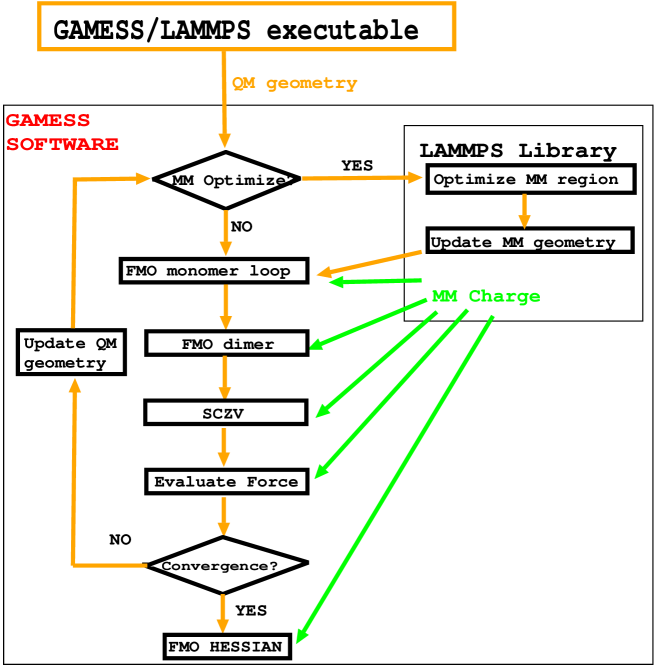
Figure 1: Schematic illustration of a geometry optimization and Hessian calculation for FMO-based QM/MM.

The computational procedure is depicted in Figure 1. Geometry optimizationsFMOopt are performed with microiterations: first, MM is used to optimize MM atoms, then a single optimization step is taken to move QM atoms, followed again by an MM optimization.

A single QM (=FMO) optimization step consists of calculating fragments in the embedding potential (FMO monomer loop in Figure 1), followed by embedded calculations of fragment pairs (dimers) and self-consistent Z-vector calculations (SCZV) FMORHF needed for analytic gradients. SCZV is based on the coupled perturbed Hartree-Fock equationsGRADBOOK .

The embedding electrostatic potential (ESP) applied to QM consists of two parts: standard ESP from FMO fragments ESPPTC1 and a field of point charges from MM atoms. In this work, periodic boundary conditions for MM are not implemented.

Regarding the naming of the method, although FMO-QM/MM was used before FMOMM1 , FMO/MM is the preferred notation covering both the mechanical embedding introduced earlier FMOopt ; FMOMM2 and the electronic enbedding in this work. Alternatively, one can view the electronic embedding as a multilayer FMO MFMO , in which the lowest layer is MM.

II.2 Analytic first derivative

The total energy for QM/MM based on FMO2 for a QM system divided into $N$ fragments is

$$E=\sum_{I}^{N}E_{I}^{\prime}+\sum_{I>J}^{N}(E_{IJ}^{\prime}-E_{I}^{\prime}-E_{J}^{\prime})+\sum_{I>J}^{N}\mathrm{Tr}(\Delta\mathbf{D}^{IJ}\mathbf{V}^{IJ})$$ (1)

where $E_{I}^{\prime}$ and $E_{IJ}^{\prime}$ are the internal energies of monomer $I$ and dimer $IJ$, respectively. $\Delta\mathbf{D}^{IJ}$ is difference between the matrices of dimer and monomer electron densities. The QM contribution ${V}^{IJ}$ to ESP for fragment $X$ ($X=IJ$ or $I$) is

$$V_{ij}^{X} =\sum_{K\neq X}^{N}\left[\sum_{A\in K}\langle i\left|\frac{-Z_{A}}{|\mathbf{r}-\mathbf{R}_{A}|}\right|j\rangle+\sum_{k\in K}2(ij|kk)\right],$$ (2)

where $Z_{A}$ and $\mathbf{R}_{A}$ is the nuclear charge and coordinates of QM atom $A$, respectively. $\mathbf{r}$ is the electron coordinate. The internal energy of fragment $X$ for Hartree-Fock is

$$E_{X}^{\prime}= \sum_{i\in X}^{\mathrm{occ}}2\tilde{h}_{ii}^{X}+\sum_{i,j\in X}^{\mathrm{occ}}\left[2\left(ii|jj\right)-\left(ij|ij\right)\right]$$

$$+ \sum_{i\in X}^{\mathrm{occ}}2P_{ii}^{X}+E_{X}^{\mathrm{NR}}+\tilde{E}_{X}^{\mathrm{NR}}+E_{X}^{\mathrm{vdW}}$$ (3)

where

$$\tilde{h}_{ii}^{X} =h_{ii}^{X}+\tilde{V}_{ii}^{X}$$ (4)

where $h_{ii}^{X}$, $(ii|jj)$, and $P_{ii}$ are the core Hamiltonian, two-electron integrals, and projection operator, respectively. $E_{X}^{\mathrm{NR}}$ is the nuclear repulsion (NR) for QM atoms. $\tilde{E}_{X}^{\mathrm{NR}}$ is the Coulomb interaction between QM nuclei and MM charges, and $E_{X}^{\mathrm{vdW}}$ is the dispersion interaction between QM and MM atoms. Throughout, Roman indices ($i,j,k$ and $l$) denote molecular orbitals (MO), and Equation (3) involves occupied (occ) orbitals only. $\tilde{V}_{ii}^{X}$ is the Coulomb interaction between electrons in QM and MM point charges,

$$\tilde{V}_{ij}^{X} =\sum_{A\in\mathrm{MM}}\langle i\left|\frac{-Q_{A}}{|\mathbf{r}-\mathbf{R}_{A}|}\right|j\rangle,$$ (5)

where $Q_{A}$ and $\mathbf{R}_{A}$ are the point charge and coordinates of MM atom $A$, respectively. $\mathbf{V}^{X}$ in Equation (1) is the electrostatic interaction between fragment $X$ and the other fragments.

In this work, density functional theory (DFT) combined with MM is also developed; for this, rather trivial modifications of equations are needed and they can be inferred from earlier publications FMODFT8 ; FMO_HESS3 . Likewise, in this work, the three-body expansion of FMO (FMO3) is also developed; for this, Equation (1) is modified to include three-body corections.This addition is straightforward and can be inferred from earlier publications FMO_HESS3 .

The derivative of the total energy with respect to a QM nuclear coordinate $a$ is

$$\frac{\partial E}{\partial a}= \sum_{I}^{N}\frac{\partial E_{I}^{\prime}}{\partial a}+\sum_{I>J}^{N}(\frac{\partial E_{IJ}^{\prime}}{\partial a}-\frac{\partial E_{I}^{\prime}}{\partial a}-\frac{\partial E_{J}^{\prime}}{\partial a})$$

$$+ \sum_{I>J}^{N}\frac{\partial\mathrm{Tr}(\Delta\mathbf{D}^{IJ}\mathbf{V}^{IJ})}{\partial a},$$ (6)

The derivative of the last term in Equation (1) is evaluated essentially as in FMO without MM FMORHF but using densities polarized by MM in $\Delta\mathbf{D}^{IJ}$. The derivative of the internal energy $E_{X}^{\prime}$ is

$$\frac{\partial E_{X}^{\prime}}{\partial a} =\sum_{i\in X}^{\mathrm{occ}}\tilde{h}_{ii}^{a,X}+\sum_{ij\in X}^{\mathrm{occ}}\left[2\left(ii|jj\right)^{a}-\left(ij|ij\right)^{a}\right]$$

$$+\sum_{i\in X}^{\mathrm{occ}}2P_{ii}^{a,X}+R^{a,X}-2\sum_{ij\in X}^{\mathrm{occ}}S^{a,X}_{ji}F^{\prime X}_{ji}$$

$$+\frac{\partial E_{X}^{\mathrm{NR}}}{\partial a}+\frac{\partial\tilde{E}_{X}^{\mathrm{NR}}}{\partial a}+\frac{\partial E_{X}^{\mathrm{vdW}}}{\partial a},$$ (7)

where

$$R^{a,X} =-\sum_{m\in X}^{\mathrm{vir}}\sum_{i\in X}^{\mathrm{occ}}4U_{mi}^{a,X}V_{mi}^{X}$$ (8)

$U_{mi}^{a,X}$ is the orbital response due to the derivatives of the MO coefficients with respect to $a$. Superscript $a$ denotes derivatives with respect to $a$, e. g. in $P_{ii}^{a,X}$ The sum of $R^{a,X}$ terms for all $X$ in Equation (8) according to Equation (1) can be writtenFMORHF

$$R^{a}= \mathbf{Z}^{T}\mathbf{B}^{a}_{0}.$$ (9)

where $\mathbf{Z}$ is the Z-vector (although $\mathbf{Z}$ is a rank 2 tensor indexed by two MOs, Equation 9 is written as a scalar product of two supervectors, summing over both MO indicesFMORHF ) obtained for FMO in the SCZV method FMORHF solving the equations

$$\mathbf{A}\mathbf{Z}=\mathbf{L}$$ (10)

$\mathbf{A}$ is the orbital Hessian matrix of second derivatives of the energy with respect to MO coefficients (a rank 4 tensor). Its definition uses MO intergrals FMORHF and it is not modified explicitly for MM. $\mathbf{L}$ is the Lagrangian (a rank 2 tensor), which also does not have explicit MM contributions. $\mathbf{B}^{a}_{0}$ is a rank 2 tensor, whose definition can be found elsewhere FMORHF .

The electrostatic MM contributions enter in Equation (4) and as the two final terms Equation (7). The dispersion contribution is the last term in Equation (7). In addition, electrostatic contributions enter SCZV via the use of MM-modified one-electron Hamiltonian in Equation (4) as a contribution to $\mathbf{B}^{a}_{0}$ (basically, one adds $\tilde{V}_{ii}^{X}$ to the standard definitionFMORHF ).

II.3 Analytic second derivative

The second derivative of the total energy with respect to two QM atom coordinates $a$ and $b$ is

$$\frac{\partial^{2}E}{\partial a\partial b} =\sum_{I}^{N}\frac{\partial^{2}E_{I}^{\prime}}{\partial a\partial b}+\sum_{I>J}^{N}(\frac{\partial^{2}E_{IJ}^{\prime}}{\partial a\partial b}-\frac{\partial^{2}E_{I}^{\prime}}{\partial a\partial b}-\frac{\partial^{2}E_{J}^{\prime}}{\partial a\partial b})$$

$$+\sum_{I>J}^{N}\frac{\partial^{2}\mathrm{Tr}(\Delta\mathbf{D}^{IJ}\mathbf{V}^{IJ})}{\partial a\partial b}.$$ (11)

The second derivative of the last term is straightforward to evaluate using the FMO Hessian formulation.FMO_HESS ; FMO_HESS2 The second derivative of the internal energy $E_{X}^{\prime}$ is

$$\frac{\partial^{2}E_{X}^{\prime}}{\partial a\partial b} =\sum_{i\in X}^{{\mathrm{occ}}}\left[\tilde{h}_{ii}^{ab,X}+P_{ii}^{ab,X}+F_{ii}^{\prime ab,X}\right]$$

$$-\sum_{i\in X}^{{\mathrm{occ}}}2S_{ii}^{ab,X}\epsilon_{ii}^{X}+4\sum_{i\in X}^{{\mathrm{occ}}}\sum_{j\in X}^{{\mathrm{occ}}}S_{ji}^{b,X}S_{ij}^{a,X}\epsilon_{ii}^{X}$$

$$+\sum_{m\in X}^{{\mathrm{vir}}}\sum_{i\in X}^{{\mathrm{occ}}}U_{mi}^{b,X}\left[4F_{im}^{\prime a,X}-4S_{mi}^{a,X}\epsilon_{ii}^{X}\right.$$

$$-2\sum_{j,l\in X}^{{\mathrm{occ}}}\left.A_{jl,mi}^{X,X}S_{jl}^{a,X}\right]$$

$$-\sum_{i\in X}^{{\mathrm{occ}}}\sum_{j\in X}^{{\mathrm{occ}}}S_{ij}^{b,X}\left[2F_{ij}^{\prime a,X}-\frac{1}{2}\sum_{k,l\in X}^{{\mathrm{occ}}}A_{ij,kl}^{X,X}S_{kl}^{a,X}\right]$$

$$-\sum_{i\in X}^{{\mathrm{occ}}}\sum_{j\in X}^{{\mathrm{occ}}}S_{ij}^{a,X}\left[2F_{ij}^{\prime b,X}-\frac{1}{2}\sum_{k,l\in X}^{{\mathrm{occ}}}A_{ij,kl}^{X,X}S_{kl}^{b,X}\right]$$

$$+\frac{\partial^{2}E_{X}^{\mathrm{NR}}}{\partial a\partial b}+\frac{\partial^{2}\tilde{E}_{X}^{\mathrm{NR}}}{\partial a\partial b}+\frac{\partial^{2}E_{X}^{\mathrm{vdW}}}{\partial a\partial b}-\overline{U}^{ab,X},$$ (12)

where $S_{jl}^{X}$ is the orbital overlap. The internal Fock matrix elements are

$$F_{ij}^{\prime,X} =\tilde{h}_{ij}^{X}+\sum_{k\in X}^{\mathrm{occ}}\left[2\left(ij|kk\right)-\left(ij|kk\right)\right]+P_{ij}^{X}.$$ (13)

The orbital response contribution $\overline{U}^{ab,X}$ in Equation (13) cancels out when all monomer and dimer contributions are added. FMO_HESS

To implement QM/MM, the standard FMO Hessian is modified taking into account the charge contribution via Equation (4), NR and vdW terms in Equation (12). In addition, CPHF equations solved for monomers and dimers in order to obtain orbital resposes $U^{a,X}_{mi}$ in Equation (12) also include the electrostatic contribution via the use of the MM-modified one-electron Hamiltonian in Equation (4).

II.4 Frozen domain formulation

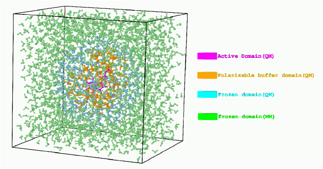
Figure 2: Combination of FMO/FDD with MM.

In the frozen domain formulation of FMO, all fragments are divided into the active A, polarizable buffer B and frozen F domains (Figure 2). Only some atoms in A can be optimized; all atoms in B and F are frozen. For the initial geometry, all fragments in all domains are calculated. During geometry optimization, B is recalculated to take into account the polarization whereas the electronic state of fragments in F is kept frozen (computed for the initial geometry only). By convention, B includes A, because fragments in A are also polarizable.

The energy of FMO/FD has an expression essentially the same as Equation (1), except that only monomers in A are included in the first sum over $I$. The most common setup is to apply the dimer (D) approximation to FD (FDD). In FMO/FDD, the dimer sum in Equation (1) is limited to those dimers where at least one of the two fragments ($I$ or $J$) belongs to A. Energy FMO_FD , its analytic first FMOFD2 and second fddhessian derivatives can be calculated for FMO/FDD.

FMO/FDD can combined with MM. The main usage of this FDD/MM approach is to add a large polarizing environment. Most typically, in this case only atoms in A can be optimized and a Hessian can be computed for them, whereas all other atoms are frozen and contribute to the polarization.

III Computational details

The analytic first and second derivative for FMO-based QM/MM were implemented into a development version of GAMESSGAMESS1 interfaced with LAMMPSLammpsPack . FMO in GAMESS was parallelized with DDIGDDI-FMO . MM calculations in LAMMPS were executed sequentially. Most simulations are performed with Hartree-Fock using the 6-31G(*) basis set (except where otherwise indicated). In DFT calculations the default Lebedev grad was used. The dispersion model D3 was employed Grimme2 . The second derivative of the dispersion energy is done by a two-point numerical differentiation. In comparisons to experiment calculated RHF frequencies were scaled SCALFAC by the factor of 0.8953.

Molecular systems were fragmented into 1 residue and molecule per fragment for the protein and water (ionic liquids), respectively. As fragmentation is shifted in FMO by one carboxyl group, to make the difference clear, fragment residues are referred to with a dash, such as Trp-6.

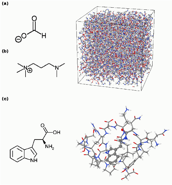
Figure 3: Molecular systems: an ionic liquid made from (a) formate anion and (b) DMEDAH cation, is shown as a box on the right. (c) Tryptophan amido acid and Trp-cage protein (Trp6 is shown with balls and thick sticks).

The accuracy of the analytic energy gradient is evaluated by comparing it with the numerical gradient for an ionic liquid consisting of formate anions and dimethylethylene-diamine (DMEDAH) cations (Figure 3-(a) and (b)). Two anions and two cations (4 fragments) are treated with QM and the rest is computed with MM; FDD is not used. The ionic liquid cluster treated in QM/MM consists of 20056 atoms.

The effect of replacing QM with MM treatment was evaluated using FMO/FDD for the Trp-cage miniprotein (PDB: 1L2Y) 1L2Y solvated in 1972 water molecules ( 6221 atoms total, Figure 3-(c)). A was set to 1 fragment, Trp-6. B and F were constructed by including all fragments within 6.5 and 20 Å from Trp-6, respectively. F was computed with a smaller basis set STO-3G. The remaining water (outside 20 Å) was treated in 2 ways: a) as a part of F with QM or b) with MM.

The effect of the QM region size was evaluated for the IR spectra of an ionic liquid and Trp-cage using FMO/FDD. Three types of calculations were done: a) setting one formate anion as A in the ionic liquid cluster, b) setting one DMEDAH cation as A in the ionic liquid cluster, c) setting Trp-6 as A in solvated Trp-cage. Then, all fragments within 6.5 Å in the respective system were assigned to B. All fragments within the size of the QM region (6-20 Å) were assigned to F. Two kinds of calculations were done: a) all fragments beyond the QM size were treated with MM (envir=MM) and b) all fragments beyond the QM size were removed (envir=none).

In order to probe the effect of the environment upon the spectra of a residue (Trp-6) in Trp-cage, the results for a methyl-capped Trp residue are compared to the results for the protein in vacuum and in solution (water). For the capped residue, full unfragmented calculations were performed. For the vacuum calculation, MM was not used; for the solvated protein, MM was used for fragments beyond the QM size of 20 Å. FMO calculations with and without MM were done at the FDD level as described above, i.e., Trp-6 was assigned as A, and all residues within 6.5 Å were assigned to B.

The parallel efficiency was evaluated for the exact analytic gradient and Hessians applied to solvated Trp-cage (FDD as described above, with the QM size of 20 Å). The calculations were performed on 1 and 8 nodes (3.1 GHz, 128 GB RAM and 8 cores per node) connected by Gigabit. 0.966 GB of RAM per core were used per node.

For preparing the initial structure for FMO geometry optimizations and Hessian calculations of the ionic liquid and solvated Trp-cage, NVT molecular dynamics (MM/MD) simulations were performed for 200 ps. Then NPT simulations were done for 1 ns, and the final geometry was used in FMO. MD simulations were performed with the time step of 0.5 fs with a Nose–Hoover thermostat and the velocity Verlet integrator. AMBER99 force fieldAMBER99 ; GAFFcite was used in MD for all molecules except that for water TIP3P was used.

The geometry optimization for QM and MM was performed with the thresholds of 10^-4 hartree/bohr and 10^-6 kcal/Å, respectively. In simulating IR spectra, the Gaussian broadening FMORaman was used with the broadening parameter of 10 cm^-1, with the exception of the solvated Trp-cage protein, for which 100 different structures were extracted from an NPT MD trajectory (one geometry every 10 ps), the geometry for each structure was optimized, Hessian computed, and the 100 discrete IR spectra were combined into one total IR spectrum.

IV Results and Discussion

IV.1 Accuracy

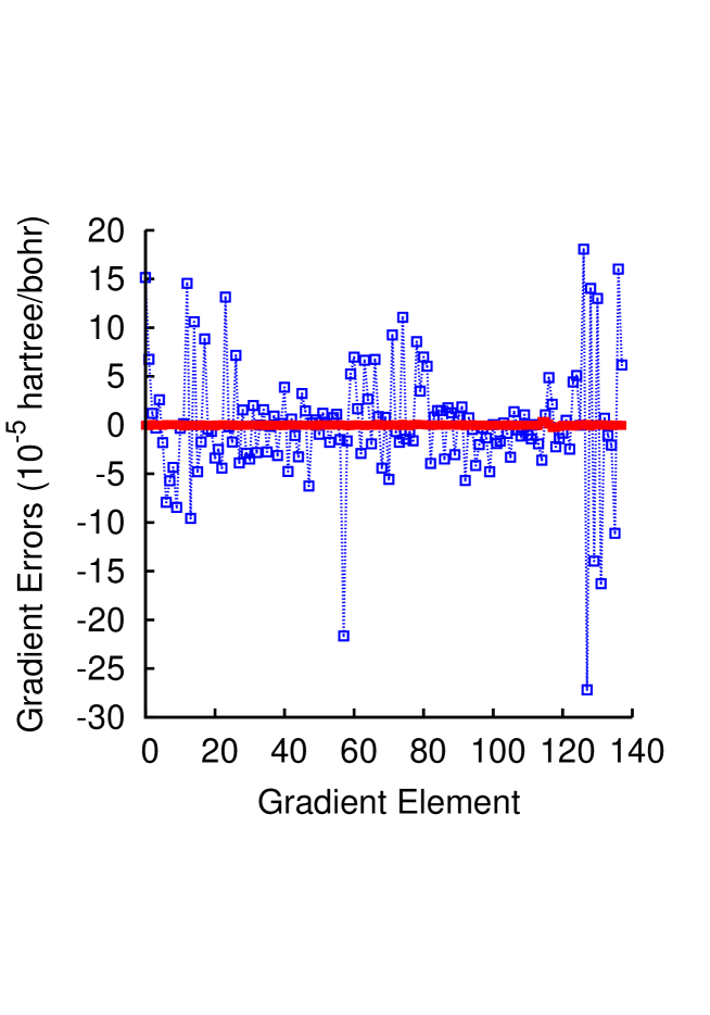
Figure 4: Accuracy of the exact and approximate (neglecting the response term in Eq. 9) analytic gradients for FMO-based QM/MM with respect to numerical gradient for an ionic liquid, shown as red solid (exact) and blue dashed (approximate) lines. Gradient elements on the x-axis are plotted for x, y and z cooridnates of all atoms consequently.

Three kinds of gradients were computed for an ionic liquid with 4 fragments in the QM refion: a) exact analytic, b) approximate analytic and c) numerical gradients. The latter gradient was used as the reference to measure the accuracy of the exact analytic gradient, and to show the importance of the response terms in Equation ( 7), neglected in the approximate gradient. The results are shown in in Figure 4 and TABLE 1. The exact gradient is accurate (agrees with the numerical gradient), whereas approximate gradient neglecting response terms has an error of about $3\times 10^{-4}$ hartree/bohr, which is larger than the default threshold for geometry optimizations by a factor of 3. Neglecting response terms can lead to energy oscillations in geometry optimization and unreliable MD simulations.FMOMD1 ; FMORHF

In order to evaluate the fragmentation accuracy, FMO-based QM/MM calculations were compared to full QM/MM calculations (where the QM region was not fragmented) at the DFT level. For this test, a water cluster was used with 9 and 365 water molecules in QM and MM regions, respectively. The results are shown in TABLE 2. The accuracy of FMO is reasonable.

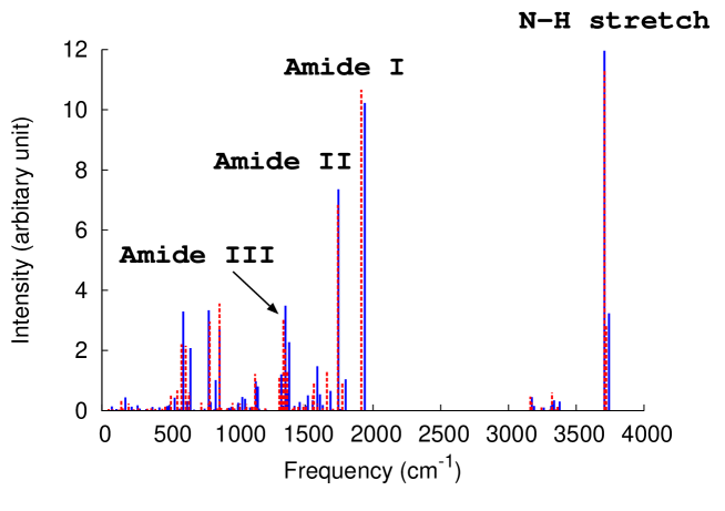
Figure 5: Effect of replacing some QM water with MM in solvated Trp-cage (envir=MM). Full QM and QM/MM IR spectra are shown as blue solid and red dashed lines, respectively.

The effect of replacing QM with MM was also evaluated with the Trp-cage protein solvated in explicit water (the protein was treated with QM, and only the treatment of some water molecules was switched from QM to MM). The IR spectra are shown in Figure 5. There is a good agreement both in terms of frequences and intensities. The main peaks are listed in TABLE 2. The largest deviation is 25 cm^-1.

IV.2 Effects of the electrostatic embedding on IR spectra

IR spectra describing vibrations in a single fragment (treated as active domain A) were computed for the DMEDAH-formate ionic liquid and Trp-cage protein, varying the QM region size. FMO(envir=MM) results for a range of QM sizes show the effect of replacing QM with MM (comparison of non-polarizable vs polarizable embedding). FMO(envir=none) results for a range of QM sizes show the effect of polarization (how removing outward fragments changes the results). It should be noted that both FMO(envir=MM) and FMO(envir=none) have exactly the same FMO/FDD setup (A+B+F), dependent on the QM region size, whereas fragments beyond F are either treated with MM (envir=MM) or neglected (envir=none).

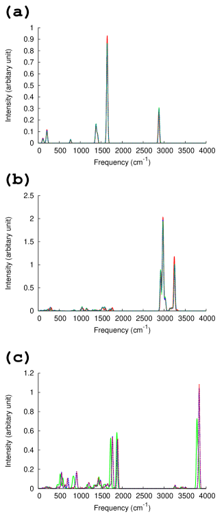
Figure 6: IR spectra of (a) one formate anion in the ionic liquid, (b) one DMEDAH cation the ionic liquid, and (c) Trp-6 in Trp-cage. For formate and DMEDAH, spectra are plotted for the QM sizes of 6.0 Å (green dashed line), 12.0 Å (blue dotted line), and 20.0 Å (red solid line). For Trp-6, spectra are plotted the QM sizes of 8.0 Å (green dashed line), 15.0 Å (blue dotted line), and 20.0 Å (red solid line).

The effect of the QM region size upon spectra in FMO(envir=MM) is shown in Figure 6. Overall, a good agreement is observed, indicating that a non-polarizable MM describes the electrostatic embedding of the active fragment well compared to QM. For Trp-6 the effect is slightly larger, up to about 30 cm^-1 in the frequency.

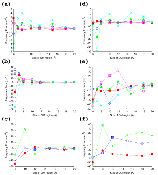
Figure 7: Deviations of the vibrational frequencies from the reference (20 Å, envir=MM) for (a) formate (envir=MM), (b) DMEDAH (envir=MM), (c) Trp-6 (envir=MM). (d) formate (envir=none), (e) DMEDAH (envir=none), and (f) Trp-6 (envir=none). Formate and DMEDAH are computed in an ionic liquid cluster; Trp-6 is computed in solvated Trp-cage.

The effect of the environment on frequencies is shown in Figure 7 and TABLE 3, where the deviations from the reference (QM size of 20 Å, envir=MM) are computed for 5 most important peaks in each system. Formate has small deviations not exceeding 10 cm^-1, and DMEDAH and Trp-6 have deviations up to 60 cm^-1.

For envir=MM, the results quickly converge as the QM size increases: for the sizes larger than 10 Å, the deviations are less than 20 cm^-1. This means that the force field is adequate for such domain sizes and well reproduces QM results.

For envir=none, much larger QM sizes are needed; for the ionic liquid, the results converge at about 20 Å, and for Trp-6 at the largest computed size of 20 Å there is still a deviation of about 30 cm^-1. The large error for Trp-6 is attributed to water molecules, and tryptophan is quite sensitive to the surrounding environment.

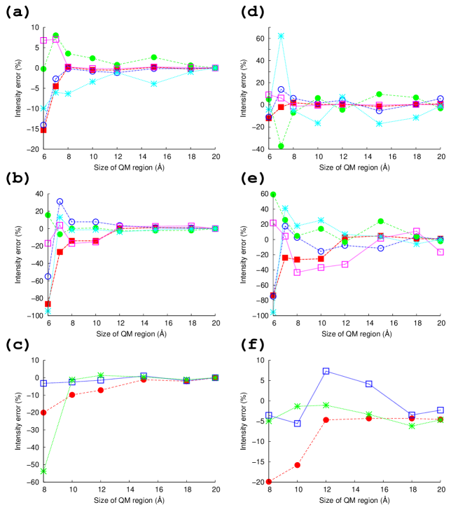
Figure 8: Deviations of the IR intensities from the reference (20 Å, envir=MM) for (a) formate (envir=MM), (b) DMEDAH (envir=MM), (c) Trp-6 (envir=MM). (d) formate (envir=none), (e) DMEDAH (envir=none), and (f) Trp-6 (envir=none). Formate and DMEDAH are computed in an ionic liquid cluster; Trp-6 is computed in solvated Trp-cage.

Intensities (Figure 8 and TABLE 4), behave in a way similar to frequencies: quickly converge for envir=MM, and feature oscillations for envir=none. For the ionic liquid, envir=none has residual errors of about 16% at 20 Å.

This indicates that adding environment with MM is a good way to improve the accuracy of the IR spectra: with the QM size of 15 Å, the largest deviation is about 6 cm^-1 in frequencies. For 15 Å in solvated Trp-cage, there are 1138 atoms in the QM region, which makes an application of a conventional QM/MM Hessian problematic. In this work, FMO/FDD is used to efficiently optimize geometry and compute Hessian for such QM region size, and relative errors in intensities are 3.9 %.

IV.3 Effect of the protein and water environment upon vibrations

In order to investigate how the surrounding environment affects the vibration frequencies in tryptophan, four different calculations were performed for (a) only the tryptophan molecule caped with methyls, (b) Trp-cage protein in gas phase, (c) Trp-cage protein in water (at one minimum) (d) Trp-cage protein in water (combining 100 conformation from MD).

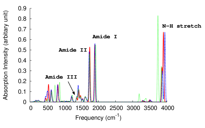
Figure 9: IR spectrum of Trp in a different environment: none (green dotted line), protein (blue dashed line) and protein+water (red solid line).

The protein environment makes a substantial effect on vibrations: the largest effect is for the vibration mode of N-H stretch around 3900 cm^-1 (Figure 9), and the peak of w7 is shifted by 57 cm^-1 (TABLE 5). Comparing the computed results to experiment without the protein environment, some frequencies differ by about 50 cm^-1. Frequencies calculated for the protein in vacuum are close to solvated experiment, but the mode w18 differs by 29 cm^-1. Inclusion of water environment shifts the peak for w16 by 28 cm^-1.

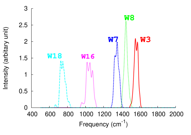
Figure 10: Computed IR spectrum for Trp-6 in solvated Trp-cage with important peaks w$i$ labelled.

For a more reliable evaluation of spectra taking into account the existence of multiple minima, 100 conformations were extracted from MD, and their structures were optimized. The computed combined spectrum is shown in Figure 10 focusing on w$i$ peaks. The vibrational modes with lower frequencies are more affected by the averaging, with a width of the peaks of about 150 cm^-1. There is some structure in the peaks (i.e., each peak is a combination of multiple peaks) that would be absent in a simple averaged broadening. The largest change due to averaging is about 13 cm^-1 (w3), smaller than the effect of the electrostatic influence of the environment (TABLE 5). For the 5 peaks, the leargest deviation from experiment is for w18, 17 cm^-1.

IV.4 Parallel efficiency

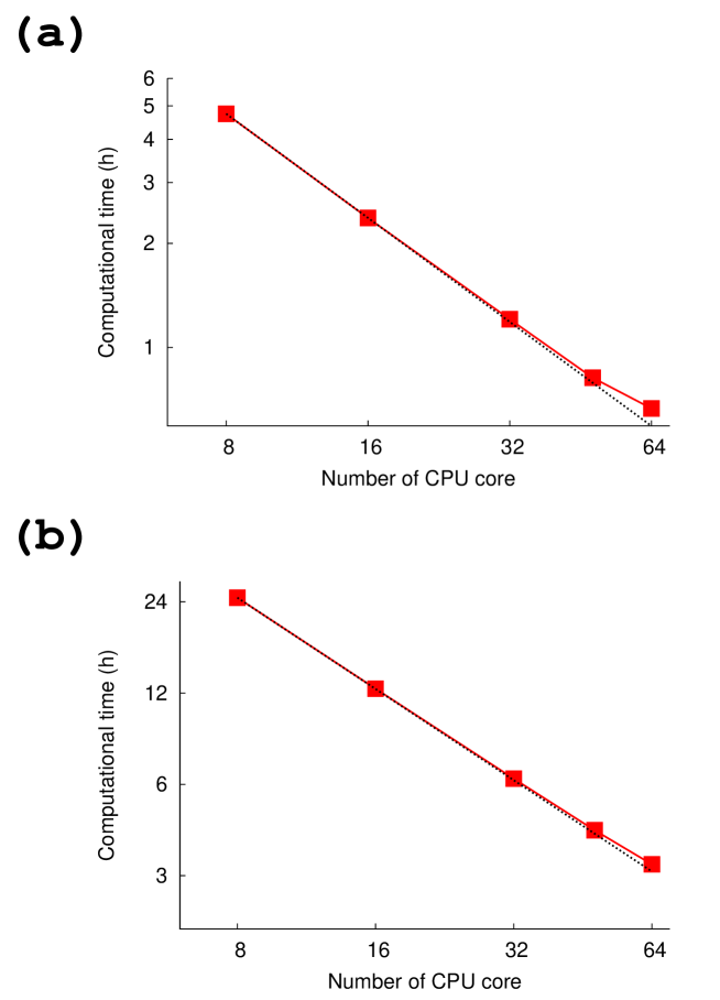
Figure 11: Wall-clock timing for FMO based QM/MM (a) gradient and (b) Hessian measured for Trp-cage solvated in explicit water: red solid and blue dashed lines show the measured and ideal results, respectively.

The parallel efficiency of the developed FMO/MM method is evaluated for both analytic gradient and Hessian using the Trp-cage protein in explicit water with the QM size of 20 Å, evaluated on a PC cluster using 8-64 cores. The timing results are shown in Figure 11.

A single point gradient calculation takes 4.74 and 0.66 hours on 8 and 64 cores, respectively, with a speedup of 7.18 on an 8-fold increase in CPU cores, corresponding to the parallel efficiency of 88.95 %. The Hessian takes 24 and 3.26 hours on 8 and 64 cores, respectively, achieving teh parallel speedup of 7.36 and the parallel efficiency of 94.69 %.

V Conclusion

The analytic energy gradient and Hessian for the electronic embedding in FMO/MM have been developed and implemented into GAMESS interfaced with LAMMPS. The importance of the response terms for obtaining an accurate gradient needed for optimizations and MD has been demonstrated. The atomic types and parameters can be easily set up using tools in LAMMPS, making it possible to do practical applications of FMO/MM.

It has been shown that replacing the QM treatment of some part of the system by MM gives accurate IR spectra provided that the size of the QM region is large enough (15 Å or more). On the other hand, simply neglecting a part of the environment results in substantial errors.

The role of the environment on IR spectra of proteins has been clearly shown: both the protein and solvent make substantial shifts. The developed method is practically applicable to studying vibrations of a chosen part of a protein while treating a large part of it with QM and the rest with MM, with a possibility to take into account multiple minima by considering a set of conformations from MD. A single point gradient and a Hessian calculation take 0.66 and 3.3 hours on 64 CPU cores, so that these simulations are practically feasible. Another advantage of FMO is that less memory is typically needed than for unfragmented calculations, because the main memory consuming step, CPHF equations, are performed for individual fragments in the field of the whole system.

Vibrations in the binding pocket of a protein binding a ligand can provide valuable information about the structure in solution. In addition, it is possible to use vibrational frequencies for estimating zero point energy and the vibrational contribution to the Gibbs free energy,FMO_HESS which can be used for increasing the accuracy of the predictions of a transition state barrier in enzymes or protein-ligand binding energies.FMOsawada1 Although unharmonic corrections are not explicitly evaluated, they can be approximately corrected for using the frequency scaling.SCALFAC

There is a substantial interest in applications of FMO to ionic liquids ionl1 ; ionl2 ; ionl3 and proteins. The ability to quickly calculate IR spectra and refine transition states in enzymatic reaction enzyme facilitated by the combination of the frozen domain FMO and MM can be useful in future applications.

TABLE captions.

Table 1: Accuracy of the approximate and analytic gradient of FMO based QM/MM, evaluated in comparison to numerical gradient (in hartree/bohr) for the formate+DMEDAH ionic liquid.

	approximatea	exact
Maximum error	0.00027171	0.00000368
RMSE	0.00006088	0.00000065

^a Neglecting the response terms in eq 9.

Table 2: Frequencies (cm^-1) and intensities (Debye²/(mass Ų) for prominent IR peaks in the solvated Trp-cage protein, computed with FMO/FDD

	water B3LYP-D
mode	FMO3/MMa		QM/MMa
mode	frequency	intensity	frequency	intensity
sym H-O-H bending	1752	4.23	1752	4.27
sym O-H stretch	3680	7.49	3680	7.40
asym O-H stretch	3792	3.72	3792	3.66
	1l2y HF-D
mode	QM/MMb		all QMc
mode	frequency	intensity	frequency	intensity
Amide III	1339	3.0	1354	3.4
Amide II	1740	6.8	1745	7.3
Amide I	1914	10.6	1939	10.2
N-H stretch	3708	11.3	3707	11.9

^a 9 and 365 water molecules are treated with QM and MM, respectively. ^b 368 and 1604 water molecules are treated with QM and MM, respectively. ^c 1972 water molecules are treated with QM.

Table 3: Maximum difference (Max) and RMSD of vibrational frequencies (cm^-1) taking the (envir=MM) results for the QM size $R$ (Å) of 20 Å as the reference.

	envir=MM		envir=none
$R$	Max	RMSD	Max	RMSD
formate in ionic liquid
20	0.0	0.0	1.2	0.8
18	0.5	0.3	6.5	3.3
15	2.2	1.2	10.6	5.0
12	0.8	0.4	4.5	2.2
10	2.0	1.0	9.6	4.6
8	4.1	2.0	3.6	2.0
7	2.8	1.3	33.8	17.4
6	5.0	3.2	9.7	4.8
DMEDAH in ionic liquid
20	0.0	0.0	7.8	4.1
18	2.4	1.1	12.1	6.7
15	1.7	1.1	17.4	9.7
12	1.9	1.4	31.8	18.0
10	7.0	4.4	38.2	26.5
8	7.5	4.6	42.7	20.0
7	23.4	14.0	33.6	16.2
6	65.0	37.2	43.3	32.8
Trp-6 in Trp-cage
20	0.0	0.0	30.6	15.5
18	6.4	4.7	34.6	19.1
15	1.7	1.1	33.2	16.4
12	18.2	9.1	30.4	15.6
10	65.2	36.1	37.6	29.6
8	51.2	36.4	54.4	40.9

Table 4: Maximum difference (Max) and RMSD of vibrational intensities (%) taking the (envir=MM) results for the QM size $R$ (Å) of 20 Å as the reference.

	envir=MM		envir=none
$R$	Max	RMSD	Max	RMSD
formate in ionic liquid
20	0.0	0.0	5.6	2.9
18	1.0	0.5	11.5	6.0
15	3.9	2.1	17.1	9.1
12	1.2	0.8	7.0	4.2
10	3.4	1.9	16.5	7.9
8	6.3	3.2	7.0	4.8
7	8.0	6.0	62.2	33.1
6	15.3	10.7	12.1	8.9
DMEDAH in ionic liquid
20	0.0	0.0	16.5	7.5
18	3.1	1.7	11.0	6.1
15	2.7	1.8	24.0	12.2
12	3.7	2.8	32.6	15.4
10	15.4	9.9	36.8	24.8
8	17.0	10.4	43.2	24.1
7	31.2	19.6	41.0	25.5
6	94.8	63.3	95.5	69.4
Trp-6 in Trp-cage
20	0.0	0.0	4.7	4.0
18	2.0	1.7	6.2	4.8
15	1.1	0.9	4.3	4.0
12	7.2	4.3	7.3	5.1
10	9.8	5.9	15.8	9.7
8	53.8	33.2	19.9	12.0

Table 5: Vibrational frequencies (cm^-1) in Trp-cage using the experimental notation w$i$.1L2yvib

method	environment	w3	w8	w7	w16	w18
HF	nonea	1530	1492	1415	995	740
FMO-HF	proteina	1540	1442	1358	993	737
FMO-HF/MM	protein+watera	1567	1440	1357	1021	742
FMO-HF/MM	protein+waterb	1554	1449	1351	1018	748
expt1L2yvib	protein+water	1558	1450	1365	1014	765

^a For a single minimum ^b Combining results from 100 conformations.

Figure captions

References

- (1) P. Pulay, Mol. Phys. 17, 197 (1969).
- (2) A. Warshel and M. Karplus, J. Am. Chem. Soc. 94, 5612 (1972).
- (3) J. A. McCammon, B. R. Gelin, and M. Karplus, Nature 267, 590 (1972).
- (4) S. Dapprich, I. Komáromi, K. S. Byun, K. Morokuma, and M. J. Frisch, J. Mol. Str.: THEOCHEM 461, 1 (1999).
- (5) K. Schwinn, N. Ferré, and M. Huix-Rotllant, J. Chem. Theory Comput. in press, 10.1021/acs.jctc.9b01145 (2020).
- (6) M. S. Gordon, Q. A. Smith, P. Xu, and L. V. Slipchenko, Ann. Rev. Phys. Chem. 64, 553 (2013).
- (7) D. S. N. M. Thellamurege and, F. Cui, H. Zhu, R. Lai, and H. Li, J. Comput. Chem. 34, 2816 (2013).
- (8) H. Li and J. H. Jensen, Theor. Chem. Acc. 107, 211 (2002).
- (9) A. Ghysels, D. Van Neck, V. Van Speybroeck, B. R. Brooks, and M. Waroquier, J. Chem. Phys. 130, 084107 (2009).
- (10) J. Kussmann, M. Beer, and C. Ochsenfeld, WIREs: Comput. Mol. Sci. 3, 614 (2013).
- (11) A. V. Akimov and O. V. Prezhdo, Chem. Rev. 115, 5797 (2015).
- (12) M. S. Gordon, D. G. Fedorov, S. R. Pruitt, and L. V. Slipchenko, Chem. Rev. 112, 632 (2012).
- (13) P. Otto and J. Ladik, Chem. Phys. 8, 192 (1975).
- (14) J. Gao, J. Phys. Chem. B 101, 657 (1997).
- (15) K. Kiewisch, C. R. Jacob, and J. Visscher, J. Chem. Theory Comput. 9, 2425 (2013).
- (16) J. Friedrich, H. Yu, H. R. Leverentz, P. Bai, J. I. Siepmann, and D. G. Truhlar, J. Phys. Chem. Lett. 5, 666 (2014).
- (17) J. Liu, X. Wang, J. Z. H. Zhang, and X. He, RSC Adv. 5, 107020 (2015).
- (18) M. Andrejić, U. Ryde, R. A. Mata, and P. Söderhjelm, Chem. Phys. Chem. 15, 3270 (2014).
- (19) P. K. Gurunathan, A. Acharya, D. Ghosh, D. Kosenkov, I. Kaliman, Y. Shao, A. I. Krylov, and L. V. Slipchenko, J. Phys. Chem. B 120, 6562 (2016).
- (20) K.-Y. Liu and J. M. Herbert, J. Chem. Theory Comput. 16, 475 (2020).
- (21) N. Komoto, T. Yoshikawa, Y. Nishimura, and H. Nakai, J. Chem. Theory Comput. 16, 2369 (2020).
- (22) S. Sakai and S. Morita, J. Phys. Chem. A 109, 8424 (2005).
- (23) W. Hua, T. Fang, W. Li, J.-G. Yu, and S. Li, J. Phys. Chem. A 112, 10864 (2008).
- (24) M. A. Collins, J. Chem. Phys. 141, 094108 (2014).
- (25) A. P. Rahalkar, V. Ganesh, and S. R. Gadre, J. Chem. Phys. 129, 234101 (2008).
- (26) J. C. Howard and G. S. Tschumper, J. Chem. Phys. 139, 184113 (2013).
- (27) K. Kitaura, E. Ikeo, T. Asada, T. Nakano, and M. Uebayasi, Chem. Phys. Lett. 313, 701 (1999).
- (28) D. G. Fedorov and K. Kitaura, J. Phys. Chem. A. 111, 6904 (2007).
- (29) D. G. Fedorov, T. Nagata, and K. Kitaura, Phys. Chem. Chem. Phys. 14, 7562 (2012).
- (30) S. Tanaka, Y. Mochizuki, Y. Komeiji, Y. Okiyama, and K. Fukuzawa, Phys. Chem. Chem. Phys. 16, 10310 (2014).
- (31) D. G. Fedorov, WIREs: Comp. Mol. Sc. 7, e1322 (2017).
- (32) T. Nagata, K. Brorsen, D. G. Fedorov, K. Kitaura, and M. S. Gordon, J. Chem. Phys. 134, 124115 (2011).
- (33) K. R. Brorsen, F. Zahariev, H. Nakata, D. G. Fedorov, and M. S. Gordon, J. Chem. Theory Comput. 10, 5297 (2014).
- (34) H. Nakata, T. Nagata, D. G. Fedorov, S. Yokojima, K. Kitaura, and S. Nakamura, J. Chem. Phys. 138, 164103 (2013).
- (35) H. Nakata, D. G. Fedorov, F. Zahariev, M. W. Schmidt, K. Kitaura, M. S. Gordon, and S. Nakamura, J. Chem. Phys. 142, 164103 (2015).
- (36) H. Lim, J. Chun, X. Jin, J. Kim, J. Yoon, and K. T. No, Sc. Rep. 9, 16727 (2019).
- (37) A. Heifetz, I. Morao, M. M. Babu, T. James, M. W. Y. Southey, D. G. Fedorov, M. Aldeghi, M. J. Bodkin, and A. Townsend-Nicholson, J. Chem. Theory Comput. 16, 2814 (2020).
- (38) M. Kusumoto, K. Ueno-Noto, and K. Takano, J. Comput. Chem. 41, 31 (2020).
- (39) T. Ishikawa, Int. J. Quantum Chem. , e25535 (2018).
- (40) A. Brekhov, V. Mironov, and Y. Alexeev, J. Phys. Chem. A 123, 6281 (2019).
- (41) V. Mironov, Y. Alexeev, and D. G. Fedorov, Int. J. Quantum Chem. 119, e25937 (2019).
- (42) H. Nakata, D. G. Fedorov, S. Yokojima, K. Kitaura, and S. Nakamura, J. Chem. Theory Comput. 10, 3689 (2014).
- (43) P. V. Avramov, D. G. Fedorov, P. B. Sorokin, S. Sakai, S. Entani, M. Ohtomo, Y. Matsumoto, and H. Naramoto, J. Phys. Chem. Lett. 3, 2003 (2012).
- (44) Y. Nishimoto, D. G. Fedorov, and S. Irle, J. Chem. Theory Comput. 10, 4801 (2014).
- (45) Y. Nishimoto and D. G. Fedorov, Phys. Chem. Chem. Phys. 18, 22047 (2016).
- (46) D. G. Fedorov, Y. Alexeev, and K. Kitaura, J. Phys. Chem. Lett. 2, 282 (2011).
- (47) H. Nakata, D. G. Fedorov, T. Nagata, K. Kitaura, and S. Nakamura, J. Chem. Theory Comput. 11, 3053 (2015).
- (48) T. Matsubara, F. Maseras, N. Koga, and K. Morokuma, J. Phys. Chem. 100, 2573 (1996).
- (49) D. G. Fedorov, T. Ishida, M. Uebayasi, and K. Kitaura, J. Phys. Chem. A 111, 2722 (2007).
- (50) D. G. Fedorov, N. Asada, I. Nakanishi, and K. Kitaura, Acc. Chem. Res. 47, 2846 (2014).
- (51) T. Okamoto, T. Ishikawa, Y. Koyano, N. Yamamoto, K. Kuwata, and M. Nagaoka, Bull. Chem. Soc. Japan 86, 210 (2013).
- (52) T. Nagata, D. G. Fedorov, and K. Kitaura, Theor. Chem. Acc. 131, 1136 (2012).
- (53) M. W. Schmidt, K. K. Baldridge, J. A. Boatz, S. T. Elbert, M. S. Gordon, J. H. Jensen, S. Koseki, N. Matsunaga, K. A. Nguyen, S. Su, T. L. Windus, M. Dupuis, and J. A. Montgomery, J. Comput. Chem. 14, 1347 (1993).
- (54) G. M. J. Barca, C. Bertoni, L. Carrington, D. Datta, N. De Silva, J. E. Deustua, D. G. Fedorov, J. R. Gour, A. O. Gunina, E. Guidez, T. Harville, S. Irle, J. Ivanic, K. Kowalski, S. S. Leang, H. Li, W. Li, J. J. Lutz, I. Magoulas, J. Mato, V. Mironov, H. Nakata, B. Q. Pham, P. Piecuch, D. Poole, S. R. Pruitt, A. P. Rendell, L. B. Roskop, K. Ruedenberg, T. Sattasathuchana, M. W. Schmidt, J. Shen, L. Slipchenko, M. Sosonkina, V. Sundriyal, A. Tiwari, J. L. Galvez Vallejo, B. Westheimer, M. Włoch, P. Xu, F. Zahariev, and M. S. Gordon, J. Chem. Phys. 152, 154102 (2020).
- (55) S. Plimpton, Journal of computational physics 117, 1 (1995).
- (56) Y. Yamaguchi, H. F. Schaefer III, Y. Osamura, and J. Goddard, A New Dimension to Quantum Chemistry: Analytical Derivative Methods in Ab Initio Molecular Electronic Structure Theory, Oxford University Press, New York, 1994.
- (57) T. Nakano, T. Kaminuma, T. Sato, K. Fukuzawa, Y. Akiyama, M. Uebayasi, and K. Kitaura, Chem. Phys. Lett. 351, 475 (2002).
- (58) D. G. Fedorov, T. Ishida, and K. Kitaura, J. Phys. Chem. A 109, 2638 (2005).
- (59) H. Nakata, D. G. Fedorov, S. Yokojima, K. Kitaura, and S. Nakamura, Chem. Phys. Lett. 603, 67 (2014).
- (60) H. Nakata, D. G. Fedorov, T. Nagata, K. Kitaura, and S. Nakamura, J. Chem. Theory Comput. 11, 3053 (2015).
- (61) D. G. Fedorov, R. M. Olson, K. Kitaura, M. S. Gordon, and S. Koseki, J. Comput. Chem. 25, 872 (2004).
- (62) S. Grimme, J. Antony, S. Ehrlich, and H. Krieg, J. Chem. Phys. 132, 154104 (2010).
- (63) A. P. Scott and L. Radom, J. Phys. Chem. 100, 16502 (1996).
- (64) J. W. Neidigh, R. M. Fesinmeyer, and N. H. Andersen, Nat. Struct. Biol. 9, 425 (2002).
- (65) J. Wang, P. Cieplak, and P. A. Kollman, J. Comput. Chem. 21, 1049 (2000).
- (66) J. Wang, R. M. Wolf, J. W. Caldwell, P. A. Kollman, and D. A. Case, J. Comput. Chem. 25, 1157 (2004).
- (67) Y. Komeiji, T. Nakano, K. Fukuzawa, Y. Ueno, Y. Inadomi, T. Nemoto, M. Uebayasi, D. G. Fedorov, and K. Kitaura, Chem. Phys. Lett. 372, 342 (2003).
- (68) T. Sawada, D. G. Fedorov, and K. Kitaura, J. Am. Chem. Soc. 132, 16862 (2010).
- (69) E. I. Izgorodina, J. Rigby, and D. R. MacFarlane, Chem. Commun. 48, 1493 (2012).
- (70) J. Rigby, S. B. Acevedo, and E. I. Izgorodina, J. Chem. Theory Comput. 11, 3610 (2015).
- (71) E. I. Izgorodina, Z. L. Seeger, D. L. A. Scarborough, and S. Y. S. Tan, Chem. Rev. 117, 6696 (2017).
- (72) Y. Abe, M. Shoji, Y. Nishiya, H. Aiba, T. Kishimoto, and K. Kitaura, Phys. Chem. Chem. Phys. 19, 9811 (2017).
- (73) Z. Ahmed, I. A. Beta, A. V. Mikhonin, and S. A. Asher, J. Am. Chem. Soc. 127, 10943 (2005).