Epidemic parameters for COVID-19 in several regions of India

Abstract

Bayesian analysis of publicly available time series of cases and fatalities in different geographical regions of India during April 2020 is reported. It is found that the initial apparent rapid growth in infections could be partly due to confounding factors such as initial rapid ramp-up of disease surveillance. A brief discussion is given of the fallacies which arise if this possibility is neglected. The growth after April 10 is consistent with a time independent but region dependent exponential. From this, $R_{0}$ is extracted using both known cases and fatalities. The two estimates are seen to agree in many cases; for these CFR is reported. It is seen that CFR and $R_{0}$ increase together. Some public health implications of this observation are discussed, including a target doubling interval if medical facilities are to remain adequate.

TIFR/TH/20-16

I Introduction

SARS-COV-2 is a virus which has newly entered the global human population when . As this host-parasite system evolves towards an equilibrium, its epidemiology has been studied extensively, but with some conflicting results conflict1 ; conflict2 . The true extent of its penetration into the population is as yet open to question serotesting , since testing is fairly restricted in most countries. Nor is the progression of the disease, COVID-19, or its method of spread completely clear review . Since the virus is already so widely established, it seems unlikely that it will be totally eliminated soon. So it is important to extract basic epidemiological parameters as cleanly as possible.

India has managed to geographically contain the spread of the COVID-19 epidemic with the nation-wide lock-down which started on 24 March, 2020. At the end of April the proportion of identified cases in India as a whole was a few tens per million, with 1–2 orders of magnitude more in hot spots. Even if this were wrong by an order of magnitude, it would still mean that the epidemic remains at an early stage in India. This, combined with the lock-down, presents an opportunity to examine the growth of the epidemic in multiple isolated regions which implement essentially the same policy with regard to testing. This study examines the heterogeneity in the growth rate of the disease, in several ways. First, the doubling intervals, $\tau$, of the cumulative number of identified cases, $C(t)$, and the cumulative number of fatalities, $D(t)$, is examined. From $\tau$ it is possible to extract the basic reproduction rate, $R_{0}$, within epidemic models. Marked heterogeneity are observed. After this the correlation between the case fatality ratio, CFR, and $R_{0}$ is studied.

Epidemic data, especially at the beginning is never clean. The public health system has to gear up for disease surveillance. The continuing recurrence of Cholera epidemics cholera , the spread of Dengue and Chikungunya chikungunya , the successful surveillance and elimination of Nipah nipah and Zika zika , show that India has a mixed record on epidemic surveillance. In addition to a possible lag between the beginning of the epidemic and its surveillance, there could be a problem of incomplete surveillance during the time the health service ramps up. Any examination of data has to allow for the identification of confounding factors such as these.

For the COVID-19 surveillance data, there are further cautionary remarks. The ICMR guidelines for testing icmr specify that only symptomatic cases should be tested using rRT-PCR. This part of the policy has been unchanged since the middle of March. Depending on the fraction of cases which are symptomatic, this could miss the actual prevalence of the disease in the population. Estimates of the fraction of asymptomatic infections range as high as 80% cebm , implying that, in this extreme case, the testing policy can never reveal more than 20% of the cases. The social stigma attached to COVID-19 stigma also means that some fraction of infections may be cryptic.

There are uncertainties in the statistics of fatalities also. It has been reported that in Europe and the US the number of fatalities due to COVID-19 may have been underestimated by a factor of 2–3. Indian cities have fairly complete registries of deaths, so miscounting of COVID-19 fatalities could come mainly from mistaken or incomplete reports of the cause of death. For larger regions, say districts and whole states, where most deaths happen at home and death certificates are not common million the errors in counting fatalities may be significantly larger, and hard to estimate at this time.

One point about the quality test that is developed here is that absolute numbers are not as important for it as the check that fatalities and identified cases are independently tracing the same rate of growth of the epidemic. This is expected at the beginning of the epidemic, when all epidemic models become linear, and the growth of generic measures is driven by the maximum eigenvalue of the linearized models. However, in the extraction of the CFR, the absolute counts do matter. In spite of the uncertainties, the correlation of CFR and $R_{0}$ holds important lessons for public health in the inevitable later stages of this epidemic in India, and the middle and low income countries of the world.

II Method

II.1 Data

Data has been extracted from official sources where possible. For Ahmedabad city, the data is made publicly available by the municipal council of the city ahmedabad . This well-organized site corrects data retrospectively for up to about 10 days. For Chennai city, the data has been collected from daily tweets by the municipal council chennai . For Indore city, the data was collected from daily bulletins of the Chief Medical and Health Officer and the collection is available for public use indore . For Mumbai city the data has been collated from the daily tweets by MCGM mcgm into a publicly available site prahlad . For Pune district the data was collated from the daily tweets by the district authority pune and the collection is publicly available indu . For Delhi and all other states, the data was taken from the publicly available collection at Covid19India covid19india . This site corrects data retrospectively for over a week. Only data on the cumulative number of identified cases, $C(t)$, and the cumulative number of known fatalities, $D(t)$, are used in this analysis. For this work data collection stopped on May 1, 2020, and retrospective corrections made after this are not included.

The unquantifiable parts of the errors in the counts of cases and fatalities due to COVID-19 were discussed in the previous section, along with the reasons why their estimates need not be included in this analysis. However, there is another part of the errors in the daily counts of cases and fatalities which come from backlogs of tests or hospital records. These shuffle a fraction of the numbers from one day to another, and therefore cause errors in the daily counts. As long as the number of facilities keep pace with the growth of the epidemic, these errors remain proportional to the number of cases and fatalities. Since the wait time for hospital beds for COVID-19 cases has remained roughly constant during the period of study, this argument is expected to hold. In view of this, of 20% of the reported values of $C(t)$ and $D(t)$ are assigned as errors. The specific fraction, 20%, was chosen to in order to cover the long range fluctuations visible in the time series (for example in those visible on days 3 and 13 of Figure 1). It has been seen that official reports and independent estimates of these number are generally within this range.

II.2 The doubling interval and $R_{0}$

At such an early stage in the infection, it is reasonable to assume exponential growth, i.e., doubling every $\tau$ days. Within this assumption one can check how well the lock-down is working by letting the doubling interval become time dependent. The simplest function to try is a linear change in $\tau$, i.e.,

$$C(t)={\cal C}_{0}2^{t/(\tau_{0}+t\tau_{1})},$$ (1)

and a similar set of three parameters for $C(t)$. Note that $\tau_{0}$ has dimensions of time, whereas $\tau_{1}$ is dimensionless. A fitting form with constant doubling interval was also used; this is denoted $\tau$, dropping the subscript.

The fitting procedure follows the methods of previous , with gamma distributions used as prior probability distribution functions (PDFs) for $\tau_{0}$ and ${\cal C}_{0}$. The additional parameter $\tau_{1}$ is allowed to take positive and negative values, by letting the prior PDF to be a Gaussian. For all these distributions, the widths are taken large enough that the posterior distribution is insensitive to the choice of priors.

The appendix contains details of the relation between a time varying doubling interval and time variation of the basic reproductive rate $R_{0}$. This requires choosing a model of the epidemic. Using the SEIR model, and the median interval between the appearance of symptoms and the time of fatalities, $t_{2}=17.8$ days lancet , one has

$$R_{0}^{0}=1+\frac{t_{2}\ln 2}{\tau_{0}},\qquad{\rm and}\qquad\frac{R_{0}^{1}}{T}=-\frac{2t_{2}\tau_{1}\ln 2}{\tau_{0}^{2}}.$$ (2)

When a constant $\tau$ is used, one can set $\tau_{1}=0$ in the above formulæ and write $R_{0}$ and $\tau$ instead of $R_{0}^{0}$ and $\tau_{0}$.

Exactly the same procedure is followed for fits to the time series for $D(t)$. Estimates of the median values of the parameters, along with interquartile ranges (IQR) and 95% credible intervals (CrI) are quoted for the doubling intervals as well as $R_{0}$.

II.3 The case fatality ratio

The analysis of the time series for $C(t)$ and $D(t)$ lead quite naturally to the case fatality ratio, CFR. This is defined as the ratio

$${\rm CFR\/}=D(t)/C(t).$$ (3)

If $C(t)$ is underestimated, then CFR is overestimated, and conversely, when $D(t)$ is underestimated, then CFR is also underestimated. This was regulated using a Bayesian estimator. Since the outcome is binomial, the prior PDF used is a beta distribution

$$P({\rm CFR\/})=\frac{1}{B(\alpha,\beta)}\;{\rm CFR\/}^{\alpha-1}(1-{\rm CFR\/})^{\beta-1},$$ (4)

with $\alpha=1$ and $\beta=2$. These choices make the posterior distribution insensitive to doubling or halving the values of the priors. The posterior distribution is of the same form with $\alpha=1+D(t)$ and $\beta=2+C(t)-D(t)$, with $t$ taken to be the final day of the analysis. Since $C(t)$ and $D(t)$ are both large, the following approximations for the median, $\mu$, and standard deviation, $\sigma$, may be used:

$$\mu[{\rm CFR\/}]\approx\frac{\alpha-1/3}{\alpha+\beta-2/3},\qquad{\rm and}\qquad\sigma^{2}[{\rm CFR\/}]=\frac{\alpha\beta}{(\alpha+\beta)^{2}(\alpha+\beta+1)}\,.$$ (5)

III Results

III.1 On $R_{0}$

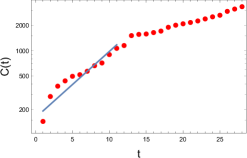
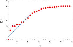
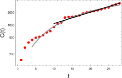
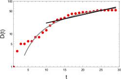
Figure 1: The time series of $C(t)$ and $D(t)$ for Delhi shown in logarithmic plot; the red dots show the data. The panels at the top show that both sets of data indicate a change of slope around day 11, i.e., about 18 days after the beginning of the national lock-down. This requires explanation. The blue lines in these panels show the most likely exponential models. The lower panels show the most likely model with changing doubling interval (gray curves) and with a constant doubling interval after day 11 (black lines).

Urb	Dates	$\tau_{0}$	$\tau_{1}$	$R_{0}^{0}$	$-R_{0}^{1}/T$
Ahmedabad	08/4–28/4	1.63	0.17	8.6	1.6
Chennai	03/4–19/4	4.94	0.19	3.5	0.2
Delhi	31/3–28/4	1.12	0.11	12.0	2.2
Indore	31/3–28/4	1.06	0.13	12.6	2.9
Mumbai	31/3–28/4	1.64	0.13	8.5	1.2
Pune	04/4–28/4	0.58	0.12	22.3	8.8

Table 1: Parameters of the most likely model describing the growth of fatalities in several urban regions (cities, except for the district of Pune). The most likely initial doubling interval $\tau_{0}$ and the linear coefficient of change $\tau_{1}$, along with estimates of the initial $R_{0}^{0}$ and its rate of change $R_{0}^{1}$. Note the extremely large values of $R_{0}^{0}$.

The time series of $C(t)$ and $D(t)$ is shown for the example of Delhi in Figure 1. Of the regions that we analysed, most cities show an initial rapid growth followed by a tempered growth. The exceptions are Ahmedabad and Chennai among cities, and the states of Gujarat, Kerala, and West Bengal. Note that day one is taken to be March 31, 2020, which is 7 days after the beginning of the national lock-down. Since $t_{2}=17.8$ days, it might be expected that the growth rate of cases in the pre-lock-down period could manifest itself in that of fatalities until around day 11. In case of a successful lock-down, $D(t)$ could then show an initial exponential growth, tempered after day 11. The initial data for fatalities in Delhi, Indore, Mumbai and Pune can indeed be described by an exponential. However, the doubling interval in Pune turns out to be half of that in Mumbai, although the average population density of Mumbai is about 6 times larger than the average in Pune city.

The ansatz of eq. (1), i.e., a linearly varying doubling interval, was also examined for urban regions. The results are collected in Table 1. In most locations the initial doubling interval seems to be between half and day and two days. When converted to $R_{0}$, one obtains extremely high values, far in excess of what has been quoted in the literature. Certainly $R_{0}$ could vary from place to place, since it depends on infectivity of the virus as well as the social networks in each location, and the latter may change from one place to another. However, $\tau_{0}$ for Pune is one third that of Mumbai, when Mumbai has six times the average population density. The wrong dependence of the doubling time for fatalities on population density, together with the observation that $C(t)$ shows a growth till the same date, supports the idea that there could be a more parsimonious explanation for this common period of growth. This is discussed in the next section. At the moment, any statistical evidence for a gradual slowing of the growth rate of the epidemic is hidden due to some confounding factors.

Data set	City	Dates	$\tau$ (days)			$R_{0}$
			med	IQR	95% CrI	med	IQR	95% CrI
Cases	Ahmedabad	11/04/20	4.32	4.24:4.42	4.11:4.55	3.86	3.81:3.92	3.71:4.01
	Chennai	10/04/20	7.52	6.87:8.25	5.92:10.2	2.70	2.55:2.85	2.27:3.13
	Delhi	11/04/20	11.7	10.7:13.0	9.00:17.0	2.10	1.99:2.21	1.80:2.42
	Indore	11/04/20	7.20	6.85:7.61	6.20:8.43	2.74	2.65:2.83	2.49:2.99
	Mumbai	10/04/20	7.35	7.00:7.72	6.45:8.47	2.70	2.62:2.78	2.46:2.94
	Pune	10/04/20	6.68	6.36:7.00	5.85:7.75	2.87	2.78:2.95	2.62:3.12
	Gujarat	11/04/20	5.30	5.06:5.55	4.68:6.09	3.35	3.24:3.46	3.05:3.65
	Kerala	31/03/20	34.5	29.7:41.0	24.0:65.0	1.39	1.34:1.45	1.24:1.55
	W.Bengal	11/04/20	6.91	6.52:7.42	5.83:8.51	2.82	2.71:2.93	2.49:3.15
Fatalities	Ahmedabad	11/04/20	4.85	4.56:5.15	4.15:5.78	3.59	3.44:3.74	3.15:4.03
	Chennai	10/04/20	8.80	8.11:9.52	7.00:11.5	2.38	2.29:2.48	2.12:2.65
	Delhi	11/04/20	12.4	11.4:13.6	9.78:16.5	2.03	1.94:2.12	1.78:2.28
	Indore	11/04/20	13.7	12.3:15.4	10.3:20.1	1.95	1.85:2.05	1.67:2.24
	Mumbai	10/04/20	9.60	8.89:10.4	7.78:12.2	2.32	2.22:2.42	2.04:2.61
	Pune	10/04/20	11.1	10.3:12.0	9.12:14.0	2.14	2.06:2.22	1.91:2.38
	Gujarat	11/04/20	5.11	4.89:5.37	4.50:5.89	3.44	3.32:3.55	3.12:3.66
	Kerala	31/03/20	24.4	22.0:27.5	18.0:36.0	1.81	1.78:1.84	1.73:1.89
	W.Bengal	11/04/20	8.01	7.28:8.73	6.30:10.5	2.62	2.48:2.75	2.22:3.01

Table 2: The stable doubling interval during the lock down, $\tau$, and the inferred basic reproduction rate, $R_{0}$, for different geographical locations in India. Shown are the median value, the inter-quartile range (IQR), and the 95% credible interval (95% CrI).

In view of this, the analysis was continued with a constant doubling interval, $\tau$, applying it to the period after day 10 or 11. For this part of the analysis data was from three states, namely Gujarat, Kerala, and West Bengal, was also used. From Figure 1, one sees that this simpler model provides as good a description of the data as the model of eq. (1). Furthermore, this yields more realistic values of $R_{0}$ implies that during the lock-down each of these places has seen a location dependent constant doubling interval. The values of $\tau$, along with inferred values of $R_{0}$, are collected in Table 2. These are the primary results of this analysis.

It was noted that the number of known cases, $C(t)$, is definitely missing cases among those who have not been tested. This could include a possibly large, fraction of asymptomatic and non-critical or pre-symptomatic cases asymptomatic ; evacu . However, India’s disease surveillance mechanism has concentrated on identifying critical cases and contact tracing, which could be a good tracer of the growth of epidemics. If this reasoning is correct, then, during the early growth of the epidemic, one should be able to obtain reliable doubling intervals from the cumulative counts of test positives previous . The results of this analysis are also given in Table 2. The two independent estimates of $R_{0}$ agree well enough that a closer look reveals interesting patterns.

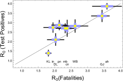
Figure 2: The values of $R_{0}$ obtained from fatalities and test positives are plotted against each other. The diagonal (thin black) line marks the locus of equal values obtained from the two series. The yellow dots mark the medians inferred from data, the thick blue bars the IQR, and the black lines the 95% CrI. The code along the bottom edge identifies each state (DL for Delhi, KL for Kerala, WB for West Bengal) or city (ad for Ahmedabad, cn for Chennai, id for Indore, mb for Mumbai, and pn for Pune). The tag is placed at the same $R_{0}$ as the corresponding city. When two cities are at nearly overlapping, then the tags are displaced vertically in the same order as the results.

The scatter plot in Figure 2 of $R_{0}$ obtained in two different ways shows several interesting patterns. First, there seem to be two groups of outbreaks. Most regions have $R_{0}$ below 3. Among the regions that we studied, Ahmedabad and Gujarat were a separate group, which saw a faster epidemic growth, with $R_{0}$ above 3. Finally there is Kerala, a different outlier, whose doubling intervals are longer than $t_{2}$, and therefore with very low values of $R_{0}$. The case of Kerala merits a separate remark. The cumulative number of fatalities reached 4 at the end of the period of study. With such low counts of fatalities the assumption of exponential growth cannot be well tested. The counts of total infections was larger, and supported the hypothesis of exponential growth over the period studied.

Second, one sees that most estimates lie close to the diagonal line. If the data was perfect, and the epidemic grew steadily, the estimates would lie exactly on this line. With this requirement we can separate the regions into two groups. One consisting of Ahmedabad, Chennai, Delhi, Gujarat, and West Bengal are, within statistical uncertainties, on this line. The second group, with Indore, Kerala, Mumbai, and Pune, are not. This could indicate some issues with the data.

On the other hand, if the data is as good as the other regions, then the fact that they are off the diagonal line should be understood. Kerala, which is the only region which lies below the diagonal, is perhaps seeing a lower growth in new cases than fatalities, which could be indicative of a gradual slowing down of the epidemic. Due to the lag by $t_{2}$, fatalities would see the slowing down later. Conversely, the regions which lie above the diagonal (namely Indore, Mumbai, and Pune, and, possibly, Chennai) could be seeing an increased growth in infections, not yet visible in fatalities because of the same time lag. Whether these scenarios are true, or the data quality is not dependable, should be known to the health agencies now, and would become visible to the public later.

III.2 On CFR

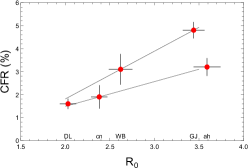
Figure 3: The values of CFR on the last day of the analysis period, plotted against $R_{0}$ obtained from fatalities. Errors on CFR are given by the standard deviation, and the error bars on $R_{0}$ indicate the IQR. One of the trend lines joins the data for cities, the other for states. The tag along the bottom identifies each state (GJ for Gujarat, WB for West Bengal) or city (DL for Delhi, ad for Ahmedabad, cn for Chennai). It is placed directly below the symbol for the corresponding region.

When there is a statistically significant difference between the doubling interval determined by $C(t)$ and $D(t)$, then the ratio gives a time-dependent CFR. This is usually understood to be a transient phenomenon. In view of this, the analysis was restricted to Ahmedabad, Chennai, Delhi, Gujarat, Kerala, and West Bengal, i.e., the regions which lie on the diagonal line of Figure 2, and therefore are seeing a steady growth of identified cases as well as fatalities. The case fatality ratios for these regions are plotted against the $R_{0}$ inferred from $D(t)$ in Figure 3.

The most obvious trend is that for the group of three cities there is an overall trend towards smaller CFR with decreasing $R_{0}$. This is also true of the two states. However, the CFR for states is displaced upwards from that for cities. Both trends have strong implications for the public health outlook and will be discussed further in the next section.

IV Discussion

Counts of known cases and fatalities of COVID-19 from five cities (Ahmedabad, Chennai, Delhi, Indore, and Mumbai), one district (Pune), and three states (Gujarat, Kerala and West Bengal) was investigated in this work. In two of the groups, there was one case each where the epidemic was not severe at the end of April (Chennai among cities, and Kerala among states). The others were known hot spots. Kerala is special because the number of fatalities is too low for statistical tests to be meaningful. There are strong regional heterogeneity in the course of the epidemic, indicating the necessity of looking at its spread at extremely local scales in order to check and control it.

IV.1 Understanding the rapid initial growth

The time series both of known cases and fatalities in four out of the six urban centers showed a rapid rise for about 18 days after the lock-down. This was followed by a much slower growth. Since fatalities track cases with a delay of 17.8 days on the average, the early part of this data could track the growth in the time before the lock-down. However, it turns out that the data grows faster in less dense urban areas. Moreover, this hypothesis is not tenable for the growth in the number of known cases.

A possibility which resolves these difficulties is that this rapid rise of numbers in the early days tracks the rapid improvement of disease surveillance rather than the epidemic. The fact that the positive cases in Kerala does not show such a rapid initial growth is consistent with reports that the state activated disease surveillance after the first infections came from abroad keralasurv . This could also be true of Ahmedabad and Gujarat, two other centers which show no such initial increase, since the state had passed through the surveillance challenge of Zika virus in recent years zika . Due to this confounding factor, it is not possible to use the data until April 10 or 11 to make any statistically valid measurement of the growth of the epidemic before the lock-down. Neglecting this leads to multiple fallacies, which I remark on next.

IV.2 Fallacies

The apparent slowing down of the growth in later stages may be falsely interpreted as a transition to polynomial growth. As shown in eq. (10) and eq. (12), this is equivalent to a time dependent doubling interval. It has been discussed in the previous subsection that this leads to highly unlikely properties of the COVID-19 epidemic.

The same apparent slowing down of the growth rate in India has also been interpreted within the homogeneous SIR model with constant, time invariant, parameters singapore . In such a simple model the time dependence can only come from early evolution towards herd immunity. This gives rise to the unlikely conclusion that herd immunity will be reached for COVID-19 while 99% of the population remains susceptible.

A misrepresentation of data also arises when “instantaneous doubling intervals” or similar measures of exponential growth are constructed using $C(t)$ for one day, or averaged over small windows of time owid . This shows a spurious gradual slowing of growth during the first three weeks of the lock-down. In later weeks these estimates are also plagued by spurious effects which result when delayed reports are dumped into cumulative numbers on one day instead of being assigned to correct past dates. These appear as evidence of local spurts or slumps in growth. Evidence of retroactive corrections from ahmedabad shows that delays of as much as ten days may occur. When these artifacts are averaged over a moving window, this gives the mistaken appearance of peaks and troughs, and may put erroneous pressure to change policies.

IV.3 Doubling time and $R_{0}$

Due to the reasons discussed in the previous subsections, the period after April 10 or 11 constitutes the base data for the main part of this analysis. As shown in Figure 1 a constant growth rate in each locality during the the lock-down models the data as well as a growth rate which changes linearly with time. This is also the most parsimonious hypothesis about the growth of the epidemic.

The observed doubling interval, and the derived quantity $R_{0}$, fall into three groups (see Table 2 and Figure 2). Several geographical regions have $R_{0}$ less than 3. Kerala has $R_{0}\simeq 1.7$ (a doubling interval larger than $t_{2}$, the interval from the emergence of symptoms to death). Gujarat and Ahmedabad have $R_{0}$ higher than 3. Since this is the growth rate during the lock-down, population density effects are unlikely to be the major determinant of $R_{0}$. It would be worthwhile to consider the role of individuals with extremely large number of contacts in this context, or a significant tail of the distribution with small number of contacts, but still above three.

Five regions pass the following data quality test— the value of $R_{0}$ obtained from the growth of fatalities and cases are equal. This does not mean that the number of cases is correctly counted. Rather it indicates that the effort to find the cases requiring critical care, and tracing their contacts has successfully resulted in tracking a constant fraction of all infected persons. It may miss, for example, a large fraction of asymptomatic cases.

IV.4 Chances of fatality

For the five geographical regions which pass the quality test described in the previous section, a further study was performed. The dependence of the case fatality ratio, CFR (i.e., the ratio of the observed number of fatalities and cases) on $R_{0}$ was investigated. Although the number of cases identified may be much smaller than the actual number of cases, the chance that cases are identified in these five regions are expected to be similar, since the rate of testing is about the same. A positive correlation between $R_{0}$ and CFR is observed.

One possible reason for this is that with lower $R_{0}$ the number of critical cases grows slower, giving medical practitioners time to figure out good practices which prevent critical care patients from progressing to fatality. Deeper studies of this factor, comparing case data from different regions, is called for in future. It is possible that this is one of the most positive, and least discussed, outcomes of the lock-down.

Another possibility may also be conjectured. Careful maintenance of social distancing, necessary to reduce $R_{0}$, results in evolutionary pressure on the virus. Lock-down and similar methods force the virus to evolve in a direction which maximizes its ability to reproduce, which it can do if the disease becomes less critical or asymptomatic, and the chances of fatality decrease. It would be interesting to compare different regions across the globe for changes in the serial time and CFR.

IV.5 Public health implications

At the observed rate of growth, and with the current rate of testing, more than 0.5% of the population in hot spots will begin to test positive for infections in about a month. A constant rate of growth of infections means that the number of hospital beds will also grow at the same rate, for as long as the epidemic is growing. Even if the rate is slowed down heavily, as it is already in Delhi, Mumbai, and Chennai, the demand for hospital facilities will keep on growing, as long as the epidemic grows.

This demand is already beginning to outstrip resources in the larger cities. The mean interval between the start of symptoms and discharge was estimated to be 24.7 days lancet . This means that unless the doubling interval is kept above 35 days ($=24.7/\ln 2$), the demand on hospitals will keep rising. Of the places we studied, only Kerala has begun to approach this break-even point.

CFR is currently small, partly because medical facilities have been able to cope with the rate of growth. If the number of cases exceeds the capacity of the medical system, cases which might have recovered will be harder to treat. Inevitably in such cases CFR will climb. It is useful to note that in Figure 3 the statewide figures for CFR are higher than those for cities. This is a reflection of the relative paucity of medical services outside cities, and is a pointer to what might happen when the number of infections rises beyond the sustainable capacity of hospitals.

V Acknowledgements

I thank Rahul Banerjee, Prahlad Harsha, D. Indumathi, and R. Shankar for sharing collated data on various cities. I thank Jayasree Subramanian for providing me with the reference ahmedabad .

Appendix A Time varying $R_{0}$ and doubling interval

In this appendix the unit of time will be taken to be the inverse of the mean rate of fatality of the infected. In these units, $R_{0}$ is the average number of new infections caused by an infected person. $R_{0}$ depends on the infectivity of the virus, as well as an average degree of the contact network. As a result, it may be affect by public health policies, such as a lock down. Say a policy measure has a time scale is $T$. Due to this, $R_{0}$ may become time-dependent, and one may write a Taylor series expansion

$$R_{0}=R_{0}^{0}+R_{0}^{1}\,\frac{t}{T}+\frac{1}{2}R_{0}^{2}\,\left(\frac{t}{T}\right)^{2}+\cdots$$ (6)

One may introduce this into a typical epidemic model equation, to obtain

$$\frac{dI}{dt}=(R_{0}-1)I,\quad{\rm which\ gives}\quad\log\left[\frac{I(t)}{I(0)}\right]=t\left[R_{0}^{0}-1+\frac{1}{2!}R_{0}^{1}\left(\frac{t}{T}\right)+\frac{1}{3!}R_{0}^{2}\left(\frac{t}{T}\right)^{2}+\cdots\right].$$ (7)

In this form of the equation time is measured in units of the case resolution time. This equation assumes that the fraction of susceptible persons is close to unity, and the fraction of persons in any other compartment is very small. As argued before, this is a reasonable assumption to make. The cumulative number of infections is then found by integration. There is no closed form result for the general case. If only the linear term in the expansion of $R_{0}$ is retained, then

$${\cal I\/}(t)=I_{0}\sqrt{\frac{\pi T}{2R_{0}^{1}}}{\rm e}^{-T(R_{0}^{0}-1)^{2}/(2R_{0}^{1})}{\rm Erfi\/}\left[\frac{T(R_{0}^{0}-1)+R_{0}^{1}t}{\sqrt{2TR_{0}^{1}}}\right].$$ (8)

The function ${\rm Erfi\/}$ is defined through the integral

$${\rm Erfi\/}(z)=\frac{2}{\sqrt{\pi}}\int_{0}^{z}dx\,{\rm e}^{x^{2}}\\$$ (9)

It is possible to use an expansion for $t\ll T$, which gives the form

$${\cal I\/}(t)={\cal I\/}(0)\frac{1}{\lambda_{0}}{\rm e}^{\lambda_{0}t}\left[1+\epsilon(1-\lambda_{0}t+\lambda_{0}^{2}t^{2})+{\cal O}(\epsilon^{2})\right]$$ (10)

where the notation $\lambda_{0}=R_{0}^{0}-1$, and $\epsilon=R_{0}^{1}/(\lambda_{0}^{2}T)$ are introduced. The imaginary part vanishes exponentially. This is easy to match to the phenomenological form

$${\cal I\/}(t)={\cal I\/}(0)\,2^{t/(\tau_{0}+\tau_{1}t/T^{\prime})}={\cal I\/}(0)\,2^{t/\tau_{0}}\left[1-\left(\frac{\ln 2\tau_{1}}{\tau_{0}^{2}T^{\prime}}\right)t^{2}+{\cal O}\left(\frac{1}{{T^{\prime}}^{2}}\right)\right],$$ (11)

where an artificial expansion parameter $T^{\prime}$ is introduced. It is set to unity after expansion. Matching these two expansions is accurate only when $\lambda_{0}t$ is large. Then

$$R_{0}^{0}=1+\frac{\ln 2}{\tau_{0}},\qquad{\rm and}\qquad\frac{R_{0}^{1}}{T}=-\frac{2\tau_{1}\ln 2}{\tau_{0}^{2}}.$$ (12)

The phenomenological parametrization of eq. (7) can be connected to the parameters of (non-autonomous) evolution equations for the epidemic. Note that $T$ and $T^{\prime}$ are both regularization scales, in the sense of a renormalization group, whose numerical value need not be specified.

In order to change units of time to days, it is necessary to choose a model of the epidemic. If one uses the SEIR model, then the unit of time would be the median interval between the appearance of symptoms and the time of fatality or recovery, whichever is earlier. This quantity, $t_{2}=17.8$ days lancet . If one instead uses the SIR model, then it is appropriate to choose the unit of time to be the median interval between the beginning of the infection and the earlier of the time of fatality or recovery. This is $t_{1}+t_{2}$, where $t_{1}$ is the median pre-symptomatic period, $t_{1}=5.1$ days. Here the conversion is made within the SEIR scheme. This gives

$$R_{0}^{0}=1+\frac{t_{2}\ln 2}{\tau_{0}},\qquad{\rm and}\qquad\frac{R_{0}^{1}}{T}=-\frac{2t_{2}\tau_{1}\ln 2}{\tau_{0}^{2}}.$$ (13)

When a constant $\tau$ is used, one can set $\tau_{1}=0$ in the above formulæ and write $R_{0}$ and $\tau$ instead of $R_{0}^{0}$ and $\tau_{0}$.

References

- (1) M.G. Boni, P. Lemey, X. Jiang, et al., Evolutionary origins of the SARS-CoV-2 sarbecovirus lineage responsible for the COVID-19 pandemic, biorXiv preprint [https://doi.org/10.1101/2020.03.30.015008]
- (2) J. Zhang, M. Litvinova, Y. Liang, et al., Changes in contact patterns shape the dynamics of the COVID-19 outbreak in China, Science, (2020) [https://doi.org/10.1126/science.abb8001]
- (3) S. Lai, N. W. Ruktanonchai, L. Zhou, et al.Effect of non-pharmaceutical interventions to contain COVID-19 in China, Nature (2020) [https://doi.org/10.1038/s41586-020-2293-x]
- (4) G. Vogel, First antibody surveys draw fire for quality, bias, Science, 368, 350–351 (2020) [DOI: 10.1126/science.368.6489.350]
- (5) H. Harapan, N. Itoh, A. Yufika, et al., Coronavirus disease 2019 (COVID-19): A literature review, J. Inf. Pub. Health, 13, 667–673, (2020) [https://doi.org/10.1016/j.jiph.2020.03.019]
- (6) M. Ali, S. Sen Gupta, N. Arora, et al., Identification of burden hotspots and risk factors for cholera in India: An observational study, PLoS ONE 12(8):e0183100 (2017) [https://doi.org/10.1371/journal.pone.0183100]
- (7) WHO, Chikunguya in India, Global Alert and Response, October (2006) [https://www.who.int/csr/don/2006_10_17/en/]
- (8) WHO, Nipah Virus — India, Emergencies Preparedness, Response, August (2018) [https://www.who.int/csr/don/07-august-2018-nipah-virus-india/en/]
- (9) WHO, Zika Virus Infection — India, Emergencies Preparedness, Response, May (2017) [https://www.who.int/csr/don/26-may-2017-zika-ind/en/]
- (10) Indian Council of Medical Research, Strategy for COVID19 testing in India, Version 4, April 9, 2020. [https://www.icmr.gov.in/pdf/covid/strategy/Strategey_for_COVID19_Test_v4_09042020.pdf]
- (11) J. Oke and C. Heneghan, Global Covid-19 Case Fatality Rates, [https:/https://www.cebm.net/covid-19/global-covid-19-case-fatality-rates//www.cebm.net/covid-19/global-covid-19-case-fatality-rates/]
- (12) Ministry of Health and Family Welfare, Government of India, Addressing Social Stigma Associated with COVID-19 Undated advisory [https://www.mohfw.gov.in/pdf/AddressingSocialStigmaAssociatedwithCOVID19.pdf]
- (13) M. Gomes, R. Begum, P. Sati, et al.Nationwide mortality studies to quantify causes of death: relevant lessons form India’s Million Death Study, Health Affairs 36 No. 11 (2017) [doi:10.1377/hlthaff.2017.0635]
- (14) Amdavad Municipal Corporation, COVID-19 website [http://covid19.ahmedabadcity.gov.in/Chart]
- (15) Greater Chennai Corporation, Official Twitter page, [https://twitter.com/chennaicorp]
- (16) R. Banerjee, Collection of Press releases by Praveen Jadiya, Chief Medical and Health Officer, Indore [https://drive.google.com/file/d/1ZLYBpaGRi_GgFCIH8CJ6XqAmszmZ3gDv/view]
- (17) Municipal Commission of Greater Mumbai, Health Department, Official handle, [https://twitter.com/mybmchealthdept?lang=en]
- (18) P. Harsha, data set available at https://docs.google.com/spreadsheets/d/1-OYukZzMlRcRKfMqh-pAle0JYAjLjUy08N9V6S51sq0/
- (19) District Information Office, Pune, Official Twitter account, [https://twitter.com/info_Pune]
- (20) D. Indumathi, data set available at https://docs.google.com/spreadsheets/d/1BDkE4S82dYSk1ZyvkKpk79a3dZy4HiOLuLp4eUZxBds/
- (21) Covid-19 India API, [https://api.covid19india.org/csv/]
- (22) R. Verity, et al., Estimates of the severity of Coronavirus disease 2019: a model based analysis, Lancet Infectious Diseases, (2020) [https://doi.org/10.1016/S1473-3099(20)30243-7]
- (23) S. Gupta, Inferring epidemic parameters for COVID-19 from fatality counts in Mumbai, preprint arXiv:2004.11677 (April, 2020) [https://arxiv.org/abs/2004.11677]
- (24) K. Mizumoto, K. Kagaya, A. Zarebski and G. Chowell, Estimating the asymptomatic proportion of coronavirus disease 2019 (COVID-19) cases on board the Diamond Princess cruise ship, Yokohama, Japan, 2020, Euro Surveill. 2020 Mar 12; 25(10): 2000180. [doi: 10.2807/1560-7917.ES.2020.25.10.2000180]
- (25) H. Nishiura, T. Kobayashi, A. Suzuki, et al., Estimation of the asymptomatic ratio of novel coronavirus infections (COVID-19), Int J Infect Dis Published Online First: 13 March 2020. [doi:10.1016/j.ijid.2020.03.020]
- (26) C. Maya, Coronavirus: Surveillance is the key, Kerala shows the way , The Hindu, 2 February, 2020. [https://www.thehindu.com/news/national/kerala/coronovirus-surveillance-is-the-key-kerala-shows-the-way/article30720140.ece]
- (27) Authors unknown, Singapore Univ. of Tech. and Design, Data Driven Innovation Lab, Predictive Monitoring of COVID-19, (Version of April 26) [https://ddi.sutd.edu.sg/]
- (28) M. Roser, H. Ritchie, E. Ortiz-Ospina and J. Hasell, Coronavirus (COVID-19) Cases Our World in Data, [https://ourworldindata.org/covid-cases]