Supplemental Materials: Spin-Nematic Vortex States in Cold Atoms

In this Supplemental Materials (SM), we provide additional information of this work. First, we provide a detailed derivation of the single-particle Hamiltonian, and then explain the symmetry and degeneracy of the single-particle spectrum at $q=0$. Additionally, we discuss the SU(3) operators and the classification of the SU(2) subspaces, and then we show the relations between the Cartesian states and the spin and nematic densities. Furthermore, we specifically display the spin and spin-nematic orders in our single-particle and many-body phase diagrams, and show how various phase transition shown in the main text are classified. Finally, we compare the main results obtained by effective 2D calculation with those obtained by 3D numerical simulations.

I Derivation of the Single-Particle Hamiltonian

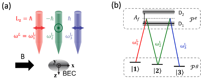
Figure S1: Detailed information on the atom-light interactions of our model. (a) Raman beams with optical frequencies $\omega^{L}_{j=1,2,3}$ and polarization on directions $\{\hat{e}_{x},\hat{e}_{y},\hat{e}_{x}\}$. Bias magnetic field is fixed along the $x$ direction. (b) Details of atomic level structures, where $\mathcal{P}^{g}$ and $\mathcal{P}^{e}$ denote the atomic ground-state and excited-state manifold. D₁ and D₂ are D-lines with electron angular quantum number $l=1$, and $A_{f}$ indicates the fine structure splitting. States $|1\rangle$, $|2\rangle$ and $|3\rangle$ are the bare atomic spin states defined by the bias field.

We provide detailed information of our proposal in Fig. S1 as a supplement of the schematic shown in the main text, where three Laguerre-Gaussian laser beams, with optical frequency $\omega^{L}_{j=1,2,3}$ and orbit angular momentum (OAM) $\hbar$, $-\hbar$ and $\hbar$, respectively, propagate along the $z$-direction and shine on a quasi-2D Bose-Einstein condensate (BEC). A bias magnetic field on the $x$-direction provides a fixed quantization axis. The ground-state ²S_1/2 and the excited manifold ²P_1/2 (D₁ line) and ²P_3/2 (D₂ line) are coupled by the Raman beams in the way as is shown in Fig. S1(b). Then, the single-particle Hamiltonian reads (we set $\hbar=m=\omega=1$ with $m$ the atomic mass, and $\omega$ the transverse trap frequency)

$$H_{0} =h_{0}+h_{\text{at}}+h_{\text{int}}$$ (S1)

$$=-\frac{1}{2}\nabla^{2}+\frac{1}{2}r^{2}+\frac{1}{2}\gamma^{2}z^{2}+\sum_{j\in g}{\omega^{g}_{j}\mathcal{P}^{g}_{j}}+\sum_{j\in e}{\omega^{e}_{j}\mathcal{P}^{e}_{j}}+A_{f}\mathbf{L}\cdot\mathbf{S}-\mathbf{d}\cdot\mathbf{E},$$

where $h_{0}$, consisting of the first five terms on the second line, is the bare Hamiltonian of the single atom with $\mathcal{P}^{g,e}=\sum_{j\in g,e}\mathcal{P}^{g,e}_{j}=\sum_{j\in g,e}\left|j\right\rangle\left\langle j\right|$ being the projection operators of the ground-state ($g$) or the excited-state ($e$) atomic manifold, and accordingly the $\omega^{g,e}_{j}$ being the energy of the ground or excited states. The term $h_{\text{at}}=A_{f}\mathbf{L}\cdot\mathbf{S}$ represents the fine structure spin-orbit coupling of the valence electron with $A_{f}$ being the fine-structure interaction strength, and the last term $h_{\text{int}}=-\mathbf{d}\cdot\mathbf{E}$ represents the atom-light electric dipole interaction with $\mathbf{E}$ the electromagnetic field, and $\mathbf{d}$ the electric dipole moment of the atom.

For the Raman process with large single-photon detuning $\omega^{e}-\omega^{g}\gg\omega^{L}$, the excited states can be adiabatically eliminated by the second-order perturbation theory Goldman2014 and the resulting effective Hamiltonian in the ground-state manifold is in the form of

$$h_{\text{eff}} =-\mathcal{P}^{g}h_{\text{int}}\mathcal{P}^{e}h_{\text{at}}^{-1}\mathcal{P}^{e}h_{\text{int}}\mathcal{P}^{g}$$ (S2)

$$=\left[u_{s}|\mathbf{E}|^{2}+iu_{v}(\mathbf{E}^{*}\times\mathbf{E})\cdot\mathbf{S}\right]\mathcal{P}^{g}.$$

$h_{\text{eff}}$ has two main effects. The first term proportional to $u_{s}\propto\left|\left\langle g|\mathbf{r}|e\right\rangle\right|^{2}/\Delta$ is the light-induced scalar shift (or ac-Stark shift) being independent on the polarization of the optical beams where $\Delta=\omega^{L}-(\omega^{g}-\omega^{e})$ is the single-photon detuning; the second term with strength $u_{v}\propto A_{f}u_{s}/\Delta$ is the light-induced vector shift. The scalar shift can be switched off as one chooses the tune-out optical frequency Schmidt2016 for the Raman beams such that the scalar shifts induced by the D₂ and D₁ transitions cancel with each other.

Properly engineering the atom-light interaction, the light-induced vector shift would lead to synthetic gauge field or synthetic spin-orbit coupling Goldman2014 . Particularly for the current Raman configuration in our scheme with $\omega_{1,3}^{L}$ being linearly polarized along the $x$-direction, and $\omega_{2}^{L}$ linearly polarized along the $y$-direction, the vector shift induced by the electromagnetic field

$$\mathbf{E} =\mathbf{E}_{1}+\mathbf{E}_{2}+\mathbf{E}_{3}$$ (S3)

$$=\left[E_{1}e^{i(\phi+\omega_{1}^{L}t)}+E_{3}e^{i(\phi+\omega_{3}^{L}t)}\right]\hat{e}_{x}+E_{2}e^{i(-\phi+\omega_{2}^{L}t)}\hat{e}_{y}+c.c.,$$

can be easily worked out as

$$h_{\text{eff}} =\left(\Omega_{12}e^{-i\delta\omega^{L}_{12}t-i2i\phi}+\Omega_{23}^{*}e^{-i\delta\omega^{L}_{32}t-2i\phi}\right)S_{z}+h.c.,$$ (S4)

where we have set $\Omega_{ij}=-iu_{v}{E_{i}^{*}E_{j}}/2$ to be the two-photon Raman frequency and $\delta\omega^{L}_{ij}=\omega^{L}_{i}-\omega^{L}_{j}$, and the $S_{z}=-(\left|1\right\rangle\left\langle 2\right|+\left|2\right\rangle\left\langle 3\right|)+h.c.$ characterizes the particle transitions in the representation of the quantized axis $S_{x}$. However, in Eq. (S4), not all the transitions are allowed by the level diagram Fig. S1(b). Neglecting the forbidden transitions and the virtual photon processes (counter-rotating-wave terms), and then by taking $\Omega_{12}=\Omega_{23}=\Omega_{R}$, we have the simplified total Hamiltonian as

$$H_{0}=-\frac{1}{2}\nabla^{2}+\frac{1}{2}r^{2}+\frac{1}{2}\gamma^{2}z^{2}+\sum_{j\in g}{\omega^{g}_{j}\mathcal{P}^{g}_{j}}+\Omega_{R}\begin{pmatrix}0&e^{-2i\phi-i\delta\omega_{12}^{L}t}&0\\ e^{2i\phi+i\delta\omega_{12}^{L}t}&0&e^{2i\phi+i\delta\omega_{32}^{L}t}\\ 0&e^{-2i\phi-i\delta\omega_{32}^{L}t}&0\end{pmatrix}.$$ (S5)

Under a standard procedure, we rewrite the Hamiltonian (S5) in a rotating frame defined by the unitary operator $U=e^{i(\delta\omega_{12}^{L}\mathcal{P}^{g}_{1}+\delta\omega_{32}^{L}\mathcal{P}^{g}_{3})t}$ as

$$H_{0}=-\frac{1}{2}\nabla^{2}+\frac{1}{2}r^{2}+\frac{1}{2}\gamma^{2}z^{2}+\begin{pmatrix}q+\delta&0&0\\ 0&0&0\\ 0&0&q-\delta\end{pmatrix}+\Omega_{R}\begin{pmatrix}0&e^{-2i\phi}&0\\ e^{2i\phi}&0&e^{2i\phi}\\ 0&e^{-2i\phi}&0\end{pmatrix},$$ (S6)

where we have used the relations $\delta=(\delta_{32}-\delta_{12})/2$ and $q=(\delta_{32}+\delta_{12})/2$ with $\delta_{ij}=\delta\omega^{L}_{ij}-(\omega_{i}^{g}-\omega_{j}^{g})$ being the two-photon detuning. Finally, a global spin rotation $S_{x}\rightarrow S_{z}$, $S_{z}\rightarrow S_{y}$ and $S_{y}\rightarrow S_{x}$ helps us to enter the commonly used $S_{z}$ representation and transforms Hamiltonian (S6) into Hamiltonian (1) in the main text.

Here, we would like to make two comments. At first, the above discussion is general and can be in principle applied to any alkaline-metal atomic species in BEC experiments. Let us take the ⁸⁷Rb atom as a specific example, which has been widely used in the experiments involving spin-orbit coupled BEC Lin2011 ; HChen2018 ; PChen2018 . For ⁸⁷Rb atom, one can choose the ground-state Zeeman levels $5^{2}$S_1/2 $\left|F=1,m_{F}=\pm 1,0\right\rangle$ and the corresponding D-line transitions $5^{2}$P_1/2 (D₁ line) and $5^{2}$P_3/2 (D₂ line) to construct the level configuration shown in the Fig. S1(b), and take $\sim 790$nm as the wave length of the Raman beams to match the tune-out wave length of ⁸⁷Rb Schmidt2016 . Furthermore, the condition $\Omega_{12}=\Omega_{23}=\Omega_{R}$ can be realized since the strength of $|E_{i=1,2,3}|\propto\sqrt{I_{i}}$ of the three Raman beams can be tuned independently, with $I_{i}$ the light intensity of the Raman beams. Secondly, note that the transverse coordinates $(r,\phi)$ and the longitudinal coordinate $z$ are decoupled in Eq. (S6), and the Raman-induced spin-orbital coupling (last term of Eq. (S6)) only lies in the transverse plane, which thus allow us to make the on-going calculations solely in the $(r,\phi)$ 2D system as were shown in the main text. In the last section of this SM, we carry out a fully 3D numerics by solving 3D Gross-Pitaevskii equations, and show the 3D results are highly consistent with those obtained by the 2D calculation.

II Spectrum At Zero Quadratic Zeeman Splitting

An apparent feature in the case of $q=0$ is that the energy spectrum of the even-parity states are symmetric about $l_{z}=1$. It means there is a symmetry only existing in the even-parity subspace of the Hamiltonian $\tilde{H}_{0}$ (Eq. (2) in the main text). The even-parity subspace is spanned by the even-parity Cartesian states $\left|y\right\rangle$ and $\left|z\right\rangle$, under which basis, $\tilde{H}_{0}$ can be written into the matrix form

$$\tilde{H}_{0}=-\frac{\partial^{2}}{2\partial r^{2}}-\frac{\partial}{2r\partial r}+\frac{r^{2}}{2}-\frac{1}{2r^{2}}\begin{bmatrix}(l_{z}-2)^{2}&0\\ 0&l_{z}^{2}\end{bmatrix}+\sqrt{2}\Omega_{R}\begin{bmatrix}0&-i\\ i&0\end{bmatrix},$$ (S7)

where we have used the relations $\nabla^{2}=\partial_{r}^{2}+\partial_{r}/r+\partial^{2}/r^{2}\partial\phi^{2}$ and $L_{z}=-i\partial_{\phi}$, and the properties of the Cartesian states that we will discuss in details in the following section.

Considering $l_{z}=1+l_{z}^{\prime}$, we have

$$\tilde{H}_{0}=-\frac{\partial^{2}}{2\partial r^{2}}-\frac{\partial}{2r\partial r}+\frac{r^{2}}{2}-\frac{1}{2r^{2}}\begin{bmatrix}(l_{z}^{\prime}-1)^{2}&0\\ 0&(l_{z}^{\prime}+1)^{2}\end{bmatrix}+\sqrt{2}\Omega_{R}\begin{bmatrix}0&-i\\ i&0\end{bmatrix},$$ (S8)

and $l_{z}=1-l_{z}^{\prime}$ which leads to

$$\tilde{H}_{0}=-\frac{\partial^{2}}{2\partial r^{2}}-\frac{\partial}{2r\partial r}+\frac{r^{2}}{2}-\frac{1}{2r^{2}}\begin{bmatrix}(l_{z}^{\prime}+1)^{2}&0\\ 0&(l_{z}^{\prime}-1)^{2}\end{bmatrix}+\sqrt{2}\Omega_{R}\begin{bmatrix}0&-i\\ i&0\end{bmatrix}.$$ (S9)

The two Hamiltonians (S8) and (S9) should have the same spectrum as they are related by a unitary transformation

$$\mathcal{U}=\begin{bmatrix}0&i\\ -i&0\end{bmatrix}.$$ (S10)

As a result, given a state with quasi-OAM $(1+l_{z}^{\prime})$, there exists a degenerate state with quasi-OAM $(1-l_{z}^{\prime})$. Hence the spectrum is symmetric about $l_{z}=1$.

III SU(3) Operators and Subspaces Classification

In the main text, we defined a series of SU(3) operators including the three spin operators $S_{\mu=x,y,z}$ and nine symmetrized nematic operators $N_{\mu\nu}=\frac{1}{2}\left(S_{\mu}S_{\nu}+S_{\nu}S_{\mu}\right)-\frac{2}{3}\delta_{\mu\nu}$. Under the basis of bare spin states $\left|\pm 1\right\rangle$ and $\left|0\right\rangle$, these operators have the following explicit matrix form:

$$S_{x} =\frac{1}{\sqrt{2}}\begin{pmatrix}0&1&0\\ 1&0&1\\ 0&1&0\end{pmatrix},\ \ \ S_{y}=\frac{i}{\sqrt{2}}\begin{pmatrix}0&-1&0\\ 1&0&-1\\ 0&1&0\end{pmatrix},\ \ \ S_{z}=\begin{pmatrix}1&0&0\\ 0&0&0\\ 0&0&-1\end{pmatrix},$$ (S11)

$$N_{xx} =\frac{1}{6}\begin{pmatrix}-1&0&3\\ 0&2&0\\ 3&0&-1\end{pmatrix},\ \ \ N_{yy}=\frac{1}{6}\begin{pmatrix}-1&0&-3\\ 0&2&0\\ -3&0&-1\end{pmatrix},\ \ \ N_{zz}=\frac{1}{3}\begin{pmatrix}1&0&0\\ 0&-2&0\\ 0&0&1\end{pmatrix},$$

$$N_{xy} =\frac{1}{2}\begin{pmatrix}0&0&i\\ 0&0&0\\ -i&0&0\end{pmatrix},\ \ \ N_{yz}=\frac{i}{2\sqrt{2}}\begin{pmatrix}0&-1&0\\ 1&0&1\\ 0&-1&0\end{pmatrix},\ \ \ N_{zx}=\frac{1}{2\sqrt{2}}\begin{pmatrix}0&1&0\\ 1&0&-1\\ 0&-1&0\end{pmatrix},$$

with $N_{yx}=N_{xy}$, $N_{zy}=N_{yz}$, and $N_{xz}=N_{zx}$ by definition. However, only eight of the above operators are linearly independent, and form a complete set of generators of the SU(3) Lie group laying as the mathematical foundation of the spin-1 quantum system.

The SU(3) group has a large number of SU(2) subgroups (or SU(2) subspaces) which are generated by triads of operators $\{\hat{O}_{i},\hat{O}_{j},\hat{O}_{k}\}$ satisfying cyclic commutation relation $[\hat{O}_{i},\hat{O}_{j}]=i\alpha\epsilon_{ijk}\hat{O}_{k}$ where $\alpha$ is the structure constant and $\epsilon_{ijk}$ is the Levi-Civita antisymmetric tensor. Root diagram obtained in the adjoint representation of the Cartan subalgebra provides a powerful way in identifying all the SU(2) subspaces Yukawa2013 . The subspaces can and can only be classified into two types with structure constant $\alpha$ being equal to 1 and 2, respectively. The most typical type-1 subspace that has received tremendous attention is the spin subspace $\mathbf{S}=\{S_{x},S_{y},S_{z}\}$ with $\alpha=1$. The spin-nematic subspace $\mathbf{Q}=\{2N_{yz},S_{x},D_{yz}=N_{yy}-N_{zz}\}$ used in the main text is of type-2 with $\alpha=2$. It has been proven that the SU(3) rotations can transform subspaces belonging to the same type, but cannot transform those belonging to different types Yukawa2013 . Since $\mathbf{Q}$ can generate a SU(2) group being isomorphic to the three-dimensional rotational group SO(3), we can treat $\mathbf{Q}$ as a vector operator. Consequently, in the space of $\mathbf{Q}$, an arbitrary three-dimensional rotation is characterized by an unitary transformation $U=e^{-i\frac{\phi}{2}\mathbf{n}\cdot\mathbf{Q}}$ with $\mathbf{n}=(n_{x},n_{y},n_{z})^{T}$ and $\phi$ corresponding to the rotational axis and the rotational angle respectively, and the factor $1/2$ in the exponent appeared due to the structure constant being $\alpha=2$.

IV Cartesian States and Spin-Nematic Density

As is shown in the main text, the Cartesian states $\left|\mu=x,y,z\right\rangle$ are eigenstates of the spin operators $S_{\mu}$ with zero eigenvalues, i.e. $S_{\mu}\left|\mu\right\rangle=0$ Ohmi1998 . The transformation matrix between the bare states and the Cartesian states is given by

$$U=\begin{pmatrix}-\frac{1}{\sqrt{2}}&\frac{i}{\sqrt{2}}&0\\ 0&0&1\\ \frac{1}{\sqrt{2}}&\frac{i}{\sqrt{2}}&0\end{pmatrix}.$$ (S12)

In the Cartesian basis, the spin and nematic operators discussed above are in quite simple forms of

$$\left\langle\mu|S_{\eta}|\nu\right\rangle=i\epsilon_{\mu\eta\nu},$$ (S13)

and

$$\left\langle\mu|N_{\eta\gamma}|\nu\right\rangle=-\frac{1}{2}(\delta_{\mu\eta}\delta_{\gamma\nu}+\delta_{\mu\gamma}\delta_{\eta\nu})+\frac{1}{3}\delta_{\mu\nu}\delta_{\eta\gamma},$$ (S14)

where subscript labels $\{\mu,\nu,\eta,\gamma\}$ can take $\{x,y,z\}$.

Consider an arbitrary state expanded using the Cartesian basis $\left|\psi\right\rangle=\sum_{\mu}m_{\mu}\left|\mu\right\rangle$, the expectation of the spin operators are

$$\mathcal{S}_{\eta} =\left\langle\psi|S_{\eta}|\psi\right\rangle$$ (S15)

$$=\sum_{\mu,\nu}m^{*}_{\mu}m_{\nu}\left\langle\mu|S_{\eta}|\nu\right\rangle$$

$$=i\sum_{\mu,\nu}m^{*}_{\mu}m_{\nu}\epsilon_{\mu\eta\nu},$$

or more compactly:

$$\boldsymbol{\mathcal{S}}=-i\mathbf{m}^{*}\times\mathbf{m};$$ (S16)

the expectation of the spin nematic operators are

$$\mathcal{N}_{\eta\gamma} =\left\langle\psi|N_{\eta\gamma}|\psi\right\rangle$$ (S17)

$$=\sum_{\mu,\nu}m^{*}_{\mu}m_{\nu}\left[-\frac{1}{2}(\delta_{\mu\eta}\delta_{\gamma\nu}+\delta_{\mu\gamma}\delta_{\eta\nu})+\frac{1}{3}\delta_{\mu\nu}\delta_{\eta\gamma}\right]$$

$$=\frac{\delta_{\eta\gamma}}{3}-\frac{1}{2}\sum_{\mu,\nu}m^{*}_{\mu}m_{\nu}(\delta_{\mu\eta}\delta_{\gamma\nu}+\delta_{\mu\gamma}\delta_{\eta\nu}),$$

$$=\frac{\delta_{\eta\gamma}}{3}-\frac{1}{2}\left(m^{*}_{\eta}m_{\gamma}+m^{*}_{\gamma}m_{\eta}\right),$$

or more compactly

$$\mathcal{N}=\frac{1}{3}-\text{Re}[\mathbf{m}^{*}\otimes\mathbf{m}],$$ (S18)

where $\otimes$ denotes the Kronecker product. With Eqs. (S16) and (S18), one can easily obtain the spin and nematic densities shown in the main text.

V Quantum Phase Transitions

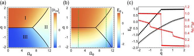
Figure S2: Single-particle phase diagrams and phase transitions. (a) Dependence of the averaged longitudinal nematic order $\left\langle\mathcal{D}_{yz}\right\rangle$ on $\Omega_{0}$ and $q$. (b) Dependence of the ground-state energy $E_{0}$ on $\Omega_{0}$ and $q$. (c) Variation of the ground-state energy $E_{0}$ (solid and dashed lines with triangles) and the its first derivative $\partial_{q}E_{0}$ (dotted and dot-dashed lines with squares) at fixed $\Omega_{0}=2$ and $\Omega_{0}=10$, as are indicated by the two green dot-dashed lines in (b), where $\partial_{q}E_{0}$ shows discontinuity at the first-order phase transition point.

In the main text, we show two phase diagrams (single-particle and many-body phases diagrams), and various quantum phase transitions that can be either first-order or second-order. Here, we present detailed information on the phase diagrams and the classification of the phase transitions.

Considering that we are dealing with the case at zero temperature $T=0$, the ground-state energy $E_{0}$ is the quantity that we are mainly interested in. Besides, since the quantum state $\boldsymbol{\Psi}$ carries both spin and spin-nematic orders, the averaged spin $\left\langle S_{\mu}\right\rangle$ and nematicity $\left\langle N_{\mu\nu}\right\rangle$ serve as macroscopic order parameters that can be used in phase identification. The averaged spin and nematicity are defined as the spatial average of the local ones, i.e.

$$\left\langle S_{\mu}\right\rangle=\int d^{2}\mathbf{r}\boldsymbol{\Psi}^{\dagger}S_{\mu}\boldsymbol{\Psi}=\int d^{2}\mathbf{r}\rho(\mathbf{r})\mathcal{S}_{\mu}(\mathbf{r}),$$ (S19)

and

$$\left\langle N_{\mu\nu}\right\rangle=\int d^{2}\mathbf{r}\boldsymbol{\Psi}^{\dagger}N_{\mu\nu}\boldsymbol{\Psi}=\int d^{2}\mathbf{r}\rho(\mathbf{r})\mathcal{N}_{\mu\nu}(\mathbf{r}),$$ (S20)

where $\mathcal{S}_{\mu}$ and $\mathcal{N}_{\mu\nu}$ are the normalized spin and nematic densities defined in Eqs. (6) and (7) in the main text.

In general, a first-order phase transition is featured by a discontinuity of the first-order derivative of $E_{0}$, and at the same time the order parameter exhibits a sudden jump; whereas a second-order transition is continuous in the first-order derivative of $E_{0}$, but is discontinuous in the second-order derivative, and in the meanwhile, the order parameter goes smoothly from a finite value to zero or vice verse. Therefore, the behaviors $E_{0}$ and the averaged spin/spin-nematic orders help us distinguish different phases as well as the order of the phase transition.

For the single-particle phase diagram shown in Fig. 2(a) in the main text, the phases I, II and III feature vanishing total spins $\left|\left\langle\mathbf{S}\right\rangle\right|$ but non-vanishing averaged nematic order. In Figs. S2(a) and (b), we reprint the single-particle phase diagram with background colors showing the variations of the longitudinal nematic order $\left\langle\mathcal{D}_{yz}\right\rangle$ and the ground-state energy $E_{0}$, respectively. One can observe that the nematic order $\left\langle\mathcal{D}_{yz}\right\rangle$ exhibits sudden jumps across the phase boundaries indicating all the transitions among phases I, II and III are of first order (labeled by solid lines). The order of the phase transitions are confirmed by examining the behavior of $E_{0}$ and $\partial_{q}E_{0}$ as functions of $q$, as shown in Fig. S2(c). In Fig. S2(c), the lines with solid markers are plotted in the case of $\Omega_{0}=2$ where the transition I-III occurs at $q=0$, and the lines with hollow markers are plotted in the case of $\Omega_{0}=10$ where two transitions III-II and II-I occur at $q\approx\pm 1$, respectively. The two cases are visually indicated by the two vertical dot-dashed lines in Fig. S2(b). It is clearly shown in the Fig. S2(c) that the energy $E_{0}$ varies continuously, but its first-order derivative $\partial_{q}E_{0}$ shows discontinuous jumps at the phase boundaries.

Similar analyses are performed on the many-body phase diagram displayed in Fig. S3, where subfigures (a)-(c) show the dependence of $\left\langle\mathcal{D}_{yz}\right\rangle$, the total spin $\left|\left\langle\mathbf{S}\right\rangle\right|=\sqrt{\left\langle S_{x}\right\rangle^{2}+\left\langle S_{y}\right\rangle^{2}+\left\langle S_{z}\right\rangle^{2}}$, and $E_{0}$ on the phase plane $\Omega_{0}$-$q$. The two emergent new phases IV and V are ferromagnetic with non-vanishing total spin, i.e. $\left|\left\langle\mathbf{S}\right\rangle\right|\neq 0$. As mentioned in the main text, these two new phases break different symmetries (Phase IV keeps the rotational symmetry but breaks the spin-parity symmetry; whereas Phase V keeps the spin-parity symmetry but breaks the rotational symmetry), and hence the phase transition between them is of first-order (denoted by solid lines), as confirmed by a sudden jump of the first-order derivative $\partial_{q}E_{0}$ across the phase boundary (not shown in the Fig. S3). In contrast, the phase transitions between the symmetry preserved phases (I, II and III) and the symmetry broken phases (IV and V) are all of the second order (denoted by dashed lines). We examine these transitions by tracking the variational amplitudes $|D_{0,1,+,-}|$ (upper panel of Fig. S3(e)), the averaged spin and spin-nematic orders (lower panel of Fig. S3(e)) and the energy behaviors (Fig. S3(f)) at $\Omega_{0}=2.5$ (indicated by the vertical dot-dashed line in Fig. S3(c)), where three transitions IV-III, III-V, and V-I occur as $q$ is ascendingly swept. The second-order transitions are clearly demonstrated in Fig. S3(f) as the second-order derivative $\partial_{q}^{2}E_{0}$ is the lowest order of derivatives that exhibits a discontinuity at the phase boundary, and at the same time the total spin order $\left|\left\langle\mathbf{S}\right\rangle\right|$ varies smoothly from a finite value to zero or from zero to a finite value. Additionally, we note that, in the limit of $\Omega_{0}\rightarrow 0$ (namely the Raman lights being switched off), the phases IV, V and I in the diagram Fig. S3(b) will reduce to the conventional ferromagnetic phase, the broken-axisymmetry phase and the polar phase of a spin-1 BEC without spin-orbit coupling Stenger1998 ; Kawaguchi2012 . These three conventional phases exist in the regimes $q<0$, $q\gtrsim 0$ and $q\gg 0$, and are featured by fully longitudinal magnetization $\left|\left\langle S_{z}\right\rangle\right|=1$, finite transverse magnetization $\left|\left\langle S_{\perp}\right\rangle\right|\neq 0$ and vanishing magnetization $\left|\left\langle\mathbf{S}\right\rangle\right|=0$, respectively.

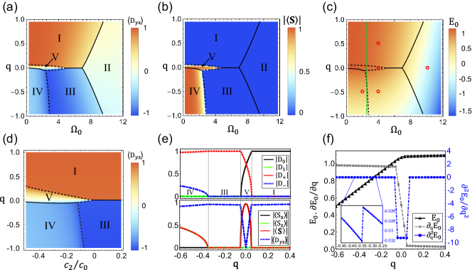
Figure S3: Many-body phase diagrams and phase transitions. (a)-(c) Many-body phase diagrams on the $\Omega_{0}$-$q$ plane with fixed $c_{2}/c_{0}=-0.1$, where the background colors in (a), (b) and (c) denote the averaged longitudinal nematic order $\left\langle\mathcal{D}_{yz}\right\rangle$, total spin order $\left|\left\langle\mathbf{S}\right\rangle\right|=\left[\left\langle S_{x}\right\rangle^{2}+\left\langle S_{y}\right\rangle^{2}+\left\langle S_{z}\right\rangle^{2}\right]^{1/2}$ and the ground-state energy $E_{0}$, respectively. Red circles in subfigure (c) indicate the typical points where the three-dimensional ground states are shown in Fig. S4. (d) Many-body phase diagram and dependence of the $\left\langle\mathcal{D}_{yz}\right\rangle$ on the $q$-$c_{2}/c_{0}$ plane, where $\Omega_{0}=2.5$ is fixed. In all the phase diagrams (a)-(d), the black solid and the black dashed lines indicate the first- and the second-order phase boundaries, respectively. (e) Variations of the variational amplitudes $|D|$, and the total spin and nematic orders on $q$. Upper panel: dependence of the variational amplitudes $|D_{0,1,+,-}|$. Lower panel: dependence of the total spin and spin-nematicity $|\left\langle S_{x}\right\rangle|$, $|\left\langle S_{z}\right\rangle|$, $\left|\left\langle\mathbf{S}\right\rangle\right|$, and $|\left\langle D_{yz}\right\rangle|$. (f) Ground-state energy $E_{0}$ and its first $\partial_{q}E_{0}$ and second derivatives $\partial_{q}^{2}E_{0}$, where $\partial_{q}E_{0}$ and $\partial^{2}_{q}E_{0}$ exhibit discontinuity at the first- and the second-order phase boundaries, respectively. Insets: a closed look at the $\partial^{2}_{q}E_{0}$ in the regime $q\in[-0.45,-0.25]$. In subfigures (e) and (f), we take $\Omega_{0}=2.5$ and $c_{2}=-0.1c_{0}$ as is indicated by the green dot-dashed line in subfigure (c).

In the above we have shown that the weak many-body interaction would lead to new phases that do not appear in the single-particle picture. The emergence of the new phases can be attributed to the interplay between the single-particle Hamiltonian $H_{0}$, the density-density interaction $c_{0}$ term and the spin-dependent interaction $c_{2}$ term in Eq.(13) of the main text. Here, let us make this point more clear by re-examining each term in the Hamiltonian. The single-particle Hamiltonian carries both rotational and spin-parity symmetry as mentioned before, which renders the single particle states to be both rotational symmetric and total-spin vanished since the local spin density $\boldsymbol{\mathcal{S}}$ (Eq.(8) in the main text) cancel with each other during the spatial average (see Fig. S3(b) and Eq. (S19)). The density-density interaction $c_{0}>0$, which is SU(3) symmetric, only tends the total density distribution $\rho(\mathbf{r})$ of the condensate to be more uniform and extended in order to minimize the density-density interaction energy. Hence, even in the case of $q=0$ where the two vortex states ($\boldsymbol{\Psi}_{+,0}$ and $\boldsymbol{\Psi}_{+,2}$) are energy degenerate, the $c_{0}$ term tends the ground state of the condensate to be one of these two states, rather than their superposition, since the superposition would break the rotational symmetry and thus make the density distribution $\rho(\mathbf{r})$ to be more localized (hence increasing interaction energy). Therefore, from this point of view, the rotational symmetry as well as the corresponding spin-nematic topology of the two vortices ($\boldsymbol{\Psi}_{+,0}$ and $\boldsymbol{\Psi}_{+,2}$) are ’protected’ by the density-density interaction $c_{0}$.

In contrast to $c_{0}$, the spin-dependent $c_{2}$ term is highly magnetization-related. This term favors anti-ferromagnetic states with vanishing macroscopic polarization if $c_{2}>0$, which is also called the anti-ferromagnetic interaction; whereas favors ferromagnetic states if $c_{2}<0$, which is thus called the ferromagnetic interaction. Consequently, the single-particle states in phase I, II and III are more preferred by $c_{2}\geq 0$ since there is no obvious confliction among the three terms ($H_{0}$, $c_{0}$, and $c_{2}$ terms) mentioned above. However if $c_{2}<0$, the $c_{2}$ term would strongly compete with the other two, since generating a state with macroscopic magnetization would either break the spin-parity symmetry which is not favored by $H_{0}$, or break the rotational symmetry which is not preferred by either $H_{0}$ or $c_{0}$ term. This competition consequently leads to the emergent new phases IV and V whose areas are highly dependent on the strength of $c_{2}$. In Fig. S3(d), we display the phase dependence on $c_{2}$ by fixing $\Omega_{0}=2.5$ and $c_{0}=1$. It is clearly shown that, the emergent phases IV and V only exist in the region of $c_{2}<0$, and the corresponding phase areas are significantly squeezed as $|c_{2}|$ decreases to zero, in accordance with the qualitative analysis above. We additionally note that, for the most commonly used alkaline metal with ferromagnetic interaction in experiments, ⁸⁷Rb for example, the intrinsic spin-exchange interaction $|c_{2}/c_{0}|$ is about $0.5\%$ Lin2011 , which is thus too weak to generate a considerable observation effect especially for the angular striped phase V. One possible solutions is to adopt the optical Feshbach resonance where $c_{2}$ is supposed to be enlarged by one order of magnitude Hamley2008 . However, the life time of the BEC will also be suppressed due to the optical heating. Another more feasible solution may be to model on pseudo-spins defined on multiple wells or optical lattice. This method has already been implemented on a spin-1/2 BEC with SOC to observe the striped phase Li2017 , where the spin-dependent interaction can be adjusted in an easier way.

VI Three-Dimensional Simulation and the Gross-Pitaevskii Equations

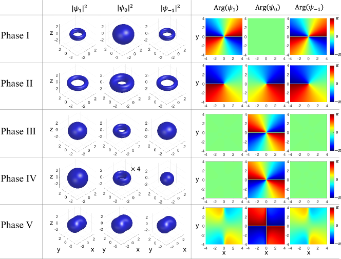
Figure S4: Density profiles and phase distributions of the three-dimensional BEC in the lab frame. Left panel: isosurface plot of the density distribution $|\psi(\mathbf{r},z)|^{2}$ in each phases, where the 1st, 2nd and 3rd column corresponds to the density distribution on the bare spin components 1, 0, and -1, respectively. Particularly for Phase IV, we enlarge the 0-component density $\psi_{0}$ by four times such that the density distribution can be clearly displayed. Right panel: the corresponding phase distribution of the many-body wave function in the x-y plane with $z=0$, i.e. $\text{Arg}(\psi_{i}(\mathbf{r},z=0))$. In our calculation, we considered an isotropic 3D harmonic confinement by taking $\gamma=\omega_{z}/\omega=1$, and $c^{\text{3D}}_{0}=\sqrt{2\pi}$ and $c_{2}^{\text{3D}}=-0.1c_{0}^{\text{3D}}$. The specific $\Omega_{0}$ and $q$ we take in each phase are: $\{\Omega_{0},q\}=\{4,0.5\}_{\text{I}}$, $\{10,0\}_{\text{II}}$, $\{4,-0.5\}_{\text{III}}$, $\{2,-0.5\}_{\text{IV}}$, $\{4,0\}_{\text{V}}$, as visually labeled out by red circles in Fig. S3(c).

Up to now, all the discussions are performed in the two-dimensional $x$-$y$ plane as mentioned in the modeling section of the main text. However, considering the recent two spin-OAM experiments HChen2018 ; PChen2018 ; Zhang2018 were done in three dimensional BEC systems, therefore we are motivated to perform a fully three-dimensional numerics by solving the coupled Gross-Pitaevskii(GP) equations and show the main physics obtained above remains valid in 3D BECs. We derive the GP equations from the total Hamiltonian $H=H_{0}+H_{\text{int}}$ in the lab frame, where $H_{0}$ and $H_{\text{int}}$ are single-particle and interacting Hamiltonian shown as Eq. (1) and Eq. (13) in the main text. Then the GP equations are explicitly given by

$$i\partial_{t}\psi_{1} =\left(-\frac{\nabla^{2}}{2}+\frac{r^{2}}{2}+\frac{\gamma^{2}z^{2}}{2}+q+\delta+c^{\text{3D}}_{0}\rho+c^{\text{3D}}_{2}\rho\mathcal{S}_{z}\right)\psi_{1}+\left(\Omega_{R}e^{-2i\phi}+\frac{c^{\text{3D}}_{2}}{\sqrt{2}}\rho\mathcal{S}_{-}\right)\psi_{0},$$ (S21)

$$i\partial_{t}\psi_{0} =\left(-\frac{\nabla^{2}}{2}+\frac{r^{2}}{2}+\frac{\gamma^{2}z^{2}}{2}+c^{\text{3D}}_{0}\rho\right)\psi_{0}+\left(\Omega_{R}e^{2i\phi}+\frac{c^{\text{3D}}_{2}}{\sqrt{2}}\rho\mathcal{S}_{+}\right)\psi_{1}+\left(\Omega_{R}e^{2i\phi}+\frac{c^{\text{3D}}_{2}}{\sqrt{2}}\rho\mathcal{S}_{-}\right)\psi_{-1},$$

$$i\partial_{t}\psi_{-1} =\left(-\frac{\nabla^{2}}{2}+\frac{r^{2}}{2}+\frac{\gamma^{2}z^{2}}{2}+q-\delta+c^{\text{3D}}_{0}\rho-c^{\text{3D}}_{2}\rho\mathcal{S}_{z}\right)\psi_{-1}+\left(\Omega_{R}e^{-2i\phi}+\frac{c^{\text{3D}}_{2}}{\sqrt{2}}\rho\mathcal{S}_{+}\right)\psi_{0},$$

where $\rho(\mathbf{r},z)=\left|\boldsymbol{\Psi}(\mathbf{r},z)\right|^{2}$ is the 3D total density,

$$\mathcal{S}_{\mu=x,y,z}(\mathbf{r},z)=\frac{\mathbf{\Psi}^{\dagger}(\mathbf{r},z)S_{\mu}\mathbf{\Psi}(\mathbf{r},z)}{\rho(\mathbf{r},z)}$$ (S22)

is the 3D normalized spin density with $\mathcal{S}_{\pm}=\mathcal{S}_{x}\pm i\mathcal{S}_{y}$, and $c^{\text{3D}}_{0,2}$ are the 3D interaction strengths, which are related to the 2D ones by $c^{\text{3D}}_{0,2}=\sqrt{2\pi/\gamma}c_{0,2}$ to a good approximation Bao2013 with $\gamma=\omega_{z}/\omega$ being the aspect ratio of the confinements. With equation Eq. (S21), we obtain the many-body ground states $\mathbf{\Psi}(\mathbf{r},z)$ by propagating the GP equations in imaginary time, which is commonly called the imaginary-time evolution. In our numerics, we deal with the temporal propagation using the time-splitting method Bao2013 , and employ the pseudo-spectral method and the finite difference method to deal with the kinetic term $-\nabla^{2}/2$ and the other non-kinetic terms, respectively.

In our GP simulation, we confine the BEC confined in a 3D isotropic harmonic trap by taking $\gamma=1$, $c^{\text{3D}}_{0}=\sqrt{2\pi}$ and $c_{2}^{\text{3D}}=-0.1c_{0}^{\text{3D}}$, and the typical ground-state density distributions as well as the transverse phase windings in each phases are displayed in Fig. S4. Specifically, in the left panel of Fig. S4, we show the isosurface plots of the density distributions $|\psi_{i=1,0,-1}(\mathbf{r},z)|^{2}$ of different bare spin components, where the specific $\{\Omega_{0},q\}$ used in the calculation are: $\{\Omega_{0},q\}=\{4,0.5\}_{\text{I}}$, $\{10,0\}_{\text{II}}$, $\{4,-0.5\}_{\text{III}}$, $\{2,-0.5\}_{\text{IV}}$, $\{4,0\}_{\text{V}}$ as visually indicated by red circles in Fig. S3(c); in the right panel of Fig. S4, we accordingly plot the transverse phase distributions at $z=0$ plane, i.e. $\text{Arg}(\psi_{i}(\mathbf{r},z=0))$. One can clearly observe in Fig. S4 that, the former four phases (I, II, III, and IV) are rotationally symmetric in the $x$-$y$ plane and each spin components carrying quantized phase windings labeled by the red numbers in Fig. 2(b) of the main text. The spin-parity symmetry breaking of phase IV is manifested as the unequal population on the $\pm 1$ components. In the phase V, where the rotational symmetry is broken, an angular striped phase is observed. Therefore, we conclude that the main physics predicted by our 2D calculation are qualitatively unchanged in a 3D BEC system.

References

• (1) N. Goldman, G. Juzeliลซnas, P. ร–hberg, and I. B. Spielman, Rep. Prog. Phys. 77, 126401 (2014).
• (2) F. Schmidt, D. Mayer, M. Hohmann, T. Lausch, F. Kindermann, and A. Widera, Phys. Rev. A 93, 022507 (2016).
• (3) Y.-J. Lin, K. Jimรฉnez-Garcรญa, and I. B. Spielman, Nature (London). 471, 83 (2011).
• (4) H.-R. Chen, K.-Y. Lin, P.-K. Chen, N.-C. Chiu, J.-B. Wang, C.-A. Chen, P.-P. Huang, S.-K. Yip, Y. Kawaguchi, and Y.-J. Lin, Phys. Rev. Lett. 121, 113204 (2018).
• (5) P.-K. Chen, L.-R. Liu, M.-J. Tsai, N.-C. Chiu, Y. Kawaguchi, S.-K. Yip, M.-S. Chang, and Y.-J. Lin, Phys. Rev. Lett. 121, 250401 (2018).
• (6) E. Yukawa, M. Ueda, and K. Nemoto, Phys. Rev. A 88, 033629 (2013).
• (7) T. Ohmi, K. Machida, J. Phys. Soc. Japan 67, 1822 (1998).
• (8) J. Stenger, S. Inouye, D.M. Stamper-Kurn, H.-J. Miesner, A.P. Chikkatur, W. Ketterle, Nature 396, 345 (1998).
• (9) K. Kawaguchi, and M. Ueda, Phys. Rep. 520, 253 (2012).
• (10) C. D. Hamley, E. M. Bookjans, G. Behin-Aein, P. Ahmadi, M. S. Chapman, Phys. Rev. A 79, 23401 (2008).
• (11) J.-R. Li, J. Lee, W. Huang, S. Burchesky, B. Shteynas, F. Cagri Top, A. O. Jamison, and W. Ketterle, Nature 543, 91 (2017).
• (12) D. Zhang, T. Gao, P. Zou, L. Kong, R. Li, X. Shen, X.-L. Chen, S.-G. Peng, M. Zhan, H. Pu, and K. Jiang, Phys. Rev. Lett. 122, 110402 (2019).
• (13) W. Bao, and Y. Cai, Kinet. Relat. Mod. 6, 1-135 (2013).