Commun. Theor. Phys.

  

Three-dimensional cytoplasmic calcium propagation with boundaries^∗

Han-Yu Jiang^1,2)  and  Jun He^1)†

¹⁾Department of Physics and Institute of Theoretical Physics, Nanjing Normal University, Nanjing, 210097, China
²⁾Sino-U.S. Center for Grazingland Ecosystem Sustainability/Pratacultural Engineering Laboratory of Gansu Province/ Key Laboratory of Grassland Ecosystem,Ministry of Education/College of Pratacultural Science, Gansu Agricultural University, Lanzhou, 730070, CHina

(Received XXXX; revised manuscript received XXXX)

Ca²⁺ plays an important role in cell signal transduction. Its intracellular propagation is the most basic process of Ca²⁺ signaling, such as calcium wave and double messenger system. In this work, with both numerical simulation and mean field ansatz, the 3-dimensional probability distribution of Ca²⁺, which is read out by phosphorylation, is studied in two scenarios with boundaries. The coverage of distribution of Ca²⁺ is found at an order of magnitude of $\mu$m, which is consistent with experimental observed calcium spike and wave. Our results suggest that the double messenger system may occur in the ER-PM junction to acquire great efficiency. The buffer effect of kinase is also discussed by calculating the average position of phosphorylations and free Ca²⁺. The results are helpful to understand the mechanism of Ca²⁺ signaling.

Keywords:

Ca²⁺ signaling, Diffusion, Gillespie algorithm, Mean field ansatz

1. Introduction

Cytoplasmic Ca²⁺ is the most basic second messenger of cell signal transduction [1, 2]. It widely involves in the regulation of cell life activities, including respondence to external stimuli, cell membrane permeability, cell secretion, metabolism and differentiation [3]. Within the cellular signaling network, the accurate decoding of diverse Ca²⁺ signal is a fundamental molecular event [4, 5]. In the double messenger system, the activity phospholipase C (PLC$\beta$) induces the hydrolysis of the phospholipid phosphatidylinositol-4, 5-bisphosphate (PIP₂) to generate inositol 1,4,5-trisphosphate (IP₃) and diacylglycerol (DAG) in the plasma membrane (PM). IP₃ mobilizes the endogenous Ca²⁺, transfers the Ca²⁺ stored in endoplasmic reticulum (ER) to the cytoplasm, and increases the intracellular Ca²⁺ concentration. Ca²⁺ combines with protein kinase C (PKC), which is a kind of calcium dependent kinase, and participates in many physiological processes, short-term physiological effects such as cell secretion and muscle contraction, or long-term physiological effects such as cell proliferation and differentiation. PKC is translocated to the inner surface of the PM, which is activated by DAG, another second messenger of phosphatidylinositol signal bound to PM. Then, the serine and threonine residues of different substrate proteins in different cell types are phosphorylated. In the current work, we define the response strength of double messenger system to stimuli as the efficiency of such signal pathway, which is described by the phosphorylation events induced near the position of the stimuli in PM. Ca²⁺ also combines with calmodulin (CaM) to form a Ca²⁺-CaM complex, which then activates the target enzymes [6]. CaM kinases are highly conserved in all eukaryotes, and are important target enzymes. It mediates many functional activities in animal and plant cells, plays an important role in the synthesis of cAMP and cGMP and degradation of glycogen, and smooths muscle contraction and neurotransmitter secretion and synthesis. Furthermore, since CaM may diffuse slowly with a speed smaller than Ca²⁺, it plays a role of buffer of the Ca²⁺ propagation to enlarge its influence coverage [7, 8].

The intracellular propagation and distribution of Ca²⁺ ion affects the activation and operation of downstream components of signaling, such as CaM and PKC [9]. According to the amplitude of the Ca²⁺ spikes, the frequency of the Ca²⁺ waves, and the microdomains of the Ca²⁺ flickers, Ca²⁺ signaling displays different temporal and spatial patterns [10, 11, 12, 13]. The distribution of intracellular Ca²⁺ is strictly regionalized, while maintaining the homeostasis of cytoplasmic Ca²⁺ is the prerequisite for normal cell growth [14]. Therefore, it is of great significance to analyze the spatial distribution and dynamic changes of intracellular Ca²⁺ for the study of cell physiological characteristics and signal transduction mechanism. In the past few decades, a variety of experimental methods were developed to measure spatial distribution of Ca²⁺ concentration in cytoplasm, endoplasmic reticulum, and other organelles. In Ref. [15], using digital imaging microscopy and the dye fura-2, distribution of intracellular cytoplasm-free Ca²⁺ were studied. The laser scanning confocal microscope technology was also developed as a research tool for observing the spatial and temporal changes of intracellular calcium distribution [16, 17]. Fluorescent indicators for Ca²⁺ are important tool to detect the Ca²⁺ [18, 19]. By using a laser scanning confocal microscope and the fluorescent calcium indicator fluo-3, Cheng and his collaborators detected the calcium sparks in heart cells [20, 21]. A plasmonic-based electrochemical impedance microscope was also developed to provide valuable information without a fluorescent labeling [22]. On the other hand, the establishment of spatial network model of calcium ion, by biochemical reaction modeling or parameter fitting, is also important to understand the spatial and temporal characteristics of calcium signal and the mechanism of signal transduction. In 2010, Rudiger and Shuai used deterministic and stochastic simulation methods to simulate a network model in which several IP₃ receptors channels release local calcium signals in a single cluster [23]. Qi established a model determined by a simple calcium kinetic equation and a Markov process [24]. The full width at half-maximum of calcium spikes was also analyzed and well reproduced in the simulation [25].

Although a lot of work has been done to study calcium spatial distribution, most of them are about calcium concentration, which is important to understand the calcium spikes and calcium waves, which usually propagate along the membrane. However, for the double messenger system, we need to know the propagation and diffusion of the calcium ion from EM to PM instead of concentration. Hence, the current understanding of the decoding mechanism of CaM and the signal network of calcium PKC still is fragmentary. Besides, little is known about the spatial location of above kinase phosphorylation events for calcium signal transduction study. In Refs. [26, 27], the authors developed a frame to estimate the accuracy of the position of external stimuli. In their work, the Ca²⁺ induced by stimuli enters the cytoplasm through a channel in membrane, and is read out by the spatial distribution of phosphorylation events in cytoplasm or membrane. It is an important reaction mechanism of the external stimuli. However, the double messenger system happens between ER and PM, which is quite different from the scenario studied in Refs. [26, 27]. Theoretically, the double messenger system should be a diffusion problem with two boundaries. Moreover, with the increase of the distance between ER and PM, the probability distribution of the Ca²⁺ becomes small, which makes the signal propagation in such pathway more difficult. The efficiency of the double messenger system should be dependent on the distance between ER and PM. The study about such issue is scarce in the literature. Hence, it is interesting to preform a study about the propagation of the Ca²⁺ perpendicular to the membrane through the phosphorylation.

By studying the random binding of calcium ions with calmodulin and relevant kinases distributed in different cytoplasmic regions, we can estimate the position of phosphorylation events in the cytoplasm or in the PM, as well as the position of binding of calcium ion to CaM / PKC and the influence domain of calcium ion through phosphorylation. Due to the short-term characteristics of calcium puff and the complexity of intracellular environment, it is difficult and cumbersome to locate the distribution area and binding probability of calcium ions by biological experiments. It is interesting to introduce theoretical model to simulate such process. Based on such new idea, by adopting mathematical simulation and mean-filed ansatz to solve non-linear diffusion equation, we start from the level of single calcium ion to study: (1) the spatial probability of Ca²⁺ read out by phosphorylation from ER to PM, which provides an overall picture of the Ca²⁺ distribution; (2) average positions of phosphorylation and the free Ca²⁺ in a direction perpendicular to the membrane, which is related to buffer effect of CaM; (3) estimation error of the readout position of phosphorylation event, which assesses the effective region of Ca²⁺. Large efficiency of double messenger system benefits from large number of phosphorylation events and small estimation error in PM. With these results, we can analyze the dependence of the efficiency of the double messenger system on the distance between ER and PM. This study provides a theoretical basis for further exploring the mechanism of Ca²⁺ mobilization induced calcium signaling pathway in cell biology, and the correlation between spatial heterogeneity of calcium ions and calcium signaling pathway.

2. Theoretical frame

In the current work, we consider CaM and PKC scenarios (see Fig. 1). Ca²⁺ enters cytoplasm through calcium pump on ER. In the CaM scenario, the phosphorylation happens in cytoplasm while the PKC attached by Ca²⁺ should be bound onto PM first in PKC scenario. In the followings, we will describe these two scenarios explicitly when presenting master equation and simulation method.

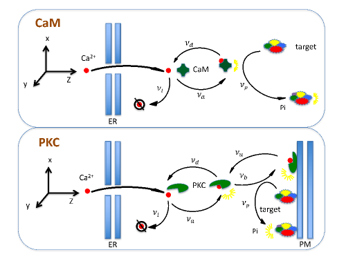
Figure 1: The CaM and PKC scenarios. The explicit description is presented in text.

2.1. Master equation

First, we present analytical description of Ca²⁺ by the master equation, with which the spatial probability distribution of phosphorylation events is introduced.

2.1.1. Diffusion of free Ca²⁺ until first attachment

In the literature, the permeation of Ca²⁺ ion in water and cytosolic was discussed [28]. Moving ion will be damped because its energy is lost to surrounding medium through viscous resistance to that movement. It can be described by using the Langevin equation [29], $m\frac{{\rm d}{\bm{v}}}{{\rm d}t}=-m\gamma{\bm{v}}+{\bm{R}}$ where the $m$, ${\bm{v}}$, and $\gamma$ are the mass, velocity and the friction coefficient of the ion, and ${\rm R}$ is random force. Average velocity deceases exponentially as $\langle{\bm{v}}\rangle=\langle{\bm{v}}\rangle_{0}{\rm e}^{-\gamma t}$. Based on the Einstein relation, the friction coefficient of the calcium ion can be evaluated as $\gamma^{-1}\approx 1$ fs [30]. It suggests that initial velocity of calcium ion will be lost in an extremely short time after entering cytoplasm. Hence, permeation of Ca²⁺ behaves as a diffusion.

We define a probability distribution function as ${\cal P}_{i_{0}}[{\bm{r}},t]$ for the state with $\rm Ca^{2+}$ ion unattached to a kinase, and we will call the Ca²⁺ in such state as “free Ca²⁺” here and hereafter. It satisfies initial condition as ${\cal P}_{i_{0}}[{\bm{r}},t=0]=\delta({\bm{r}})$ which suggests that $\rm Ca^{2+}$ ion enters system at ${\bm{r}}=0$ on ER in both scenarios, that is, we define calcium pump as the origin of coordinate. If not losing into cytosolic, the moving Ca²⁺ ion attaches and activates a kinase, CaM or PKC , and it obeys diffusion equation as,

$$\partial_{t}{\cal P}_{i_{0}}[{\bm{r}},t]=D_{C}\nabla^{2}{\cal P}_{i_{0}}[{\bm{r}},t]-(\nu_{a}+\nu_{l}){\cal P}_{i_{0}}[{\bm{r}},t],$$ (1)

where the $D_{C}$ is the diffusion constant for Ca²⁺ in cytosolic, and $\nu_{a}$ and $\nu_{l}$ are the rates of attachment and losing, respectively.

In Refs. [26, 27], Ca²⁺ ion enters and kinase binds to the same PM, which is important in the determination of position of external signal. In the current work, we consider 3-dimensional PKC scenario (see Fig. 1), which happens in the important double messenger system. It leads to obvious difference. Ca²⁺ ion enters from ER idealized as an infinite plane and diffuses in 3-dimensional space. Furthermore, PKC needs to propagate to PM as another plane at a distance $l$. Hence, the $\rm Ca^{2+}$ ion will be reflected by boundary, PM and/or ER, which leads to boundary condition as

$$\partial_{z}{\cal P}_{i_{0}}[{\bm{r}},t]|_{z=0} = 0,\quad{\rm for\ CaM\ and\ PKC,}$$ (2)

$$\partial_{z}{\cal P}_{i_{0}}[{\bm{r}},t]|_{z=l} = 0,\quad{\rm for\ PKC\ only.}$$ (3)

2.1.2. Attachment and detachment

After the first attachment, a function ${\cal P}_{a}[n({\bm{\xi}});{\bm{r}},t]$ is introduced to reflect two probabilities: having kinase activated by Ca²⁺ ion at position ${\bm{r}}$ and time $t$, and having a distribution of phosphorylation event $n({\bm{\xi}})$ at time $t$. ${\cal P}_{i}[n({\bm{\xi}});{\bm{r}},t]$ is defined analogously but with Ca²⁺ detached from the kinase. The master equation is given by

$$\partial_{t}{\cal P}_{i}[(n({\bm{\xi}});{\bm{r}},t]=D_{C}\nabla^{2}{\cal P}_{i}[n({\bm{\xi}});{\bm{r}},t]+\nu_{d}{\cal P}_{a}[n({\bm{\xi}});{\bm{r}},t]-(\nu_{a}+\nu_{l}){\cal P}_{i}[n({\bm{\xi}});{\bm{r}},t],$$ (4)

where $\nu_{d}$ is the rate of detachment.

Because $\rm Ca^{2+}$ ion and active kinase will be also reflected by boundary, we have boundary condition as

$$\partial_{z}{\cal P}_{i,a}[n({\bm{\xi}});{\bm{r}},t]|_{z=0} = 0,\quad{\rm for\ CaM\ and\ PKC,}$$ (5)

$$\partial_{z}{\cal P}_{i}[n({\bm{\xi}});{\bm{r}},t]|_{z=l} = 0,\quad{\rm for\ PKC\ only.}$$ (6)

2.1.3. Phosphorylation in CaM scenario

Difference appears after activation of kinase in two scenarios. In CaM scenario (see Fig. 1), the active kinase phosphorylates directly in cytosolic at a rate of $\nu_{p}$, which can be described as

$$\partial_{t}{\cal P}_{a}[n({\bm{\xi}});{\bm{r}},t] = D_{K}\nabla^{2}{\cal P}_{a}[n({\bm{\xi}});{\bm{r}},t]-\nu_{d}{\cal P}_{a}[n({\bm{\xi}});{\bm{r}},t]+\nu_{a}\left\{{\cal P}_{i}[n({\bm{\xi}});{\bm{r}},t]+{\cal P}_{i0}[{\bm{r}},t]\right\}$$ (7)

$$+ \nu_{p}\left\{{\cal P}_{a}[n({\bm{\xi}})-\delta({\bm{\xi}}-{\bm{r}});{\bm{r}},t]-{\cal P}_{a}[n({\bm{\xi}});{\bm{r}},t]\right\}.$$

The active kinase diffuses by constant $D_{K}$. The Dirac delta function $\delta({\bm{\xi}}-{\bm{r}})$ means that a phosphorylation event happens at ${\bm{r}}$, then, the distribution jumps from ${\cal P}_{a}[n({\bm{\xi}})-\delta({\bm{\xi}}-{\bm{r}});{\bm{r}},t]$ to ${\cal P}_{a}[n({\bm{\xi}});{\bm{r}},t]$ at a rate of $\nu_{p}$.

2.1.4. Binding and phosphorylation in PKC scenario

In PKC scenario, phosphorylation does not happen directly after attachment. The PKC attached by a Ca²⁺ diffuses and obeys a master equation

$$\partial_{t}{\cal P}_{a}[n({\bm{\xi}});{\bm{r}},t]=D_{K}\nabla^{2}{\cal P}_{a}[n({\bm{\xi}});{\bm{r}},t]-\nu_{d}{\cal P}_{a}[n({\bm{\xi}});{\bm{r}},t]+\nu_{a}\{{\cal P}_{i}[n({\bm{\xi}});{\bm{r}},t]+{\cal P}_{i_{0}}[{\bm{r}},t]\}.$$ (8)

The kinase should be bound onto PM and activated by DAG to make phosphorylation possible. A new state function ${\cal P}_{b}[n({\bm{\xi}});\bar{\bm{r}},t]$ is defined as the probability distribution, when $\rm Ca^{2+}$ attaches to a kinase and the complex binds into PM. Because PM is at a fixed distance from ER, we adopt $\bar{\bm{r}}$ to denote the ${\bm{r}}$ with $z$ equaling to a distance $l$. The binding and unbinding of PKC to PM can be written as a boundary condition is [31],

$$-D_{K}\partial_{z}{\cal P}_{a}[n({\bm{\xi}});\bar{\bm{r}},t]=\nu_{u}{\cal P}_{b}[n({\bm{\xi}});\bar{\bm{r}},t]-\nu_{b}{\cal P}_{a}[n({\bm{\xi}});\bar{\bm{r}},t],$$ (9)

where $\nu_{b}$ and $\nu_{u}$ are the rates of binding and unbinding from PM, respectively.

The phosphorylation at a rate of $\nu_{p}$ on PM follows master equation as

$$\partial_{t}{\cal P}_{b}[n({\bm{\xi}});\bar{\bm{r}},t] = \nu_{b}{\cal P}_{a}[n({\bm{\xi}});\bar{\bm{r}},t]-\nu_{u}{\cal P}_{b}[n({\bm{\xi}});\bar{\bm{r}},t]$$ (10)

$$+ \nu_{p}\{{\cal P}_{b}[n(\bar{\bm{\xi}})-\delta(\bar{\bm{\xi}}-\bar{\bm{r}});\bar{\bm{r}},t]-{\cal P}_{b}[n(\bm{\xi});\bar{\bm{r}},t]\}.$$

In both PKC and CaM scenarios, we define a probability distribution ${\cal P}_{0}[(n({\bm{\xi}});{\bm{r}},t]$ when the $\rm Ca^{2+}$ ion is lost, which obeys

$$\partial_{t}{\cal P}_{0}[n({\bm{\xi}});t]=\nu_{l}\int{\rm d}{\bm{r}}\left\{{\cal P}_{i}[n({\bm{\xi}});{\bm{r}},t]+{\cal P}_{i_{0}}[{\bm{r}},t]\right\}.$$ (11)

In summary, the CaM scenario shown in upper panel of Fig. 1 is described by diffusion equations in Eqs. (1,4,7,11) and boundary conditions in Eqs. (2,5), and the PKC scenario shown in lower panel of Fig. 1 is described by diffusion equations in Eqs. (1,4,8,11) and boundary conditions in Eqs. (2,3,5,6,9,10). Hereafter, we will make a dimensionless treatment. The time and space are scaled by $\nu_{p}$ and $\sqrt{\nu_{p}/D_{C}}$, respectively. The scaled $\nu_{a}$, $\nu_{d}$, $\nu_{l}$, and $D_{K}$ can be obtained from scaled time and space.

2.2. Stochastic simulation of master equation

With the master equation above, theoretically, we can obtain the distribution of phosphorylation event, $n(\bm{\xi})$. However, the master equations are difficult to be solved analytically. In the current work, we adopt the Gillespie algorithm to do the stochastic simulation [32, 26, 27] in 3-dimensional space with the boundary conditions.

The simulation follows scenarios shown in Fig. 1. Ca²⁺ ion enters system at ${\bm{r}}=\bm{0}$. An event occurs in a step of time $\Delta t=-lnr/(\nu_{a}+\nu_{l})$ with $r$ being a random number in a range from 0 to 1. This event is attachment or leaving system, which is determined by drawing a random number from 0 to $\nu_{l}+\nu_{a}$. If the random number is smaller than $\nu_{l}$, simulation stops. If not, the position of active kinase is changed in three directions by drawing three independent random numbers $\Delta{\bm{r}}$ from the Gaussian distribution with zero mean and variance $2\Delta t$. If obtained new position is out of the boundaries, it will be reflected by boundaries to a position in allowed region , $z>0$ for CaM scenario and $l>z>0$ for PKC scenario.

In CaM scenario, kinase may phosphorylate target protein or detach in a new step of time. The type of event is still determined by drawing a random number. At the same time, the kinase moves randomly. If phosphorylation happens, the position is recorded as ${\bm{\xi}}_{i}$. If the Ca²⁺ ion detaches from the active kinase, simulation continues to a new loop. When simulation ends, we have a trajectory of $n_{0}$ phosphorylation events. With $N$ simulations, we obtain $n$ trajectories with phosphorylation events. We would like to remind that if a simulation does not raise any phosphorylation event, we do not count it into the number of trajectories $n$.

In PKC scenario, after the kinase is activated, the situation is more complex because it has possibility to be bound onto PM. Let us consider an active kinase in $z_{old}$, which certainly locates between two boundaries, goes to a new position $z_{new}$ after a random movement at time $\Delta t$. If the $z_{new}$ is still between the two boundaries, we draw a random number $r$ between 0 and 1. If $r<e^{-[(l-z_{new})(l-z_{old})]/(D_{K}\Delta t)}\nu_{b}\sqrt{\pi\Delta t}/(2\sqrt{D_{K}})$, the kinase is bound to the membrane [33, 34]. If the $z_{new}$ is larger than $l$, the kinase is bound if $r>1-\nu_{b}\sqrt{\pi\Delta t}/(2\sqrt{D_{K}})$. Otherwise, it will be reflected. If the $z_{new}$ is smaller than 0, kinase is reflected only. If after reflecting, the kinase is still out of boundaries, the above step should be repeated until it goes to a position between the boundaries. After binding to the membrane, a random number is drawn to determine whether phosphorylation happens or kinase unbinds from the membrane. The position of phosphorylation will be recorded as in CaM scenario.

2.3. Mean-field ansatz

Now we consider mean-field ansatz (MF) where phosphorylation rate at position ${\bm{r}}$ is assumed to be proportional to the probability of finding a kinase at this position. In CaM scenario, the expected number $\hat{n}({\bm{r}})$ of phosphorylation events in the limit $t\to\infty$ is $\hat{n}({\bm{r}})=\bar{p}_{a}({\bm{r}})=\int^{\infty}_{0}dt^{\prime}p_{a}({\bm{r}},t^{\prime})$, where the barred quantities indicate time-integrated quantities [26, 27] . For Eqs. (1, 4, 7), to obtain the distribution of expected phosphorylation events, we are then left with solving,

$$-\delta({\bm{r}}) = \nabla^{2}\bar{p}_{i_{0}}({\bm{r}})-(\nu_{a}+\nu_{l})\bar{p}_{i_{0}}({\bm{r}}),$$

$$0 = \nabla^{2}\bar{p}_{i}({\bm{r}})+\nu_{d}\bar{p}_{a}({\bm{r}})-(\nu_{a}+\nu_{l})\bar{p}_{i}({\bm{r}}),$$

$$0 = D_{K}\nabla^{2}\bar{p}_{a}({\bm{r}})-\nu_{d}\bar{p}_{i}({\bm{r}})+\nu_{a}[\bar{P}_{i}({\bm{r}})+\bar{P}_{i0}({\bm{r}})].$$ (12)

The first equation can be easily solved as

$$\bar{p}_{i_{0}}(r)=e^{-\omega r}/2\pi r\equiv\hat{n}_{0}({\bm{r}}),$$ (13)

which is also the probability distribution of last position of free Ca²⁺.

Now, we need solve the two equations left which are coupled to each other. The $z$ is larger than zero for these two equations. However, due to the boundary at $z=0$ is reflective, it is reasonable to make an even extension. Hence, we can preform the Fourier transformation for three direction as,

$$0 = -D_{K}{q}^{2}\bar{p}_{a}({\bm{q}})-\nu_{d}\bar{p}_{a}({\bm{q}})+\nu_{a}[\bar{p}_{i}({\bm{q}})+\bar{p}_{i_{0}}({\bm{q}})],$$

$$0 = -{q}^{2}\bar{p}_{i}({\bm{q}})+\nu_{d}\bar{p}_{a}({\bm{q}})-\omega^{2}\bar{p}_{i}({\bm{q}}).$$ (14)

After inverse transformation, we have

$$\hat{n}({\bm{r}})=\bar{p}_{a}(r)=\frac{\nu_{a}}{D_{K}}\frac{1}{\lambda_{+}^{2}-\lambda_{-}^{2}}\frac{e^{-\lambda_{-}r}-e^{-\lambda_{+}r}}{2\pi r},$$ (15)

where $\lambda_{\pm}=\sqrt{(a\pm\sqrt{a^{2}-4b})/2}$ with $a=(\nu_{a}+\nu_{l})+{\nu_{d}}/{D_{K}}$ and $b={\nu_{l}\nu_{d}}/{D_{K}}$.

As in the CaM scenario, the distribution of phosphorylation events in PKC scenario at time $t\to\infty$ is given by $\hat{n}=\bar{p}_{b}(\bar{\bm{r}})$, which is related to kinase distribution as, $\partial_{t}p_{b}(\bar{\bm{r}})=\nu_{b}p_{a}(\bar{\bm{r}})-\nu_{u}p_{b}(\bar{\bm{r}})$ from Eq. (9). After integrating, we have

$$\hat{n}_{PKC}=\bar{p}_{b}(\bar{\bm{r}})=\frac{\nu_{b}}{\nu_{u}}\bar{p}_{a}(\bar{\bm{r}}).$$ (16)

One can finds that MF master equation in PKC scenario are the same as Eq. (12) in CaM scenario. Difference is that PKC scenario has additional boundary condition at $z=l$. It makes the Fourier transformation adopted in CaM scenario failure to solve these coupled differential equations because it only works in a region from 0 to $\infty$. Hence, in this work, we do not try to give analytical results, but present the simulation results in PKC scenario. However, for large $l$, effect of boundary at $z=l$ on master equations becomes small. If neglecting the boundary effect, the $p_{a}(\bar{\bm{r}})$ can be solved as in the CaM scenario. Combined with Eq. (16), one can expect a similar result except a factor for PKC scenario at large $l$. It can be used to check our simulation results.

3. Results

With above preparation, spatial probability distribution of phosphorylation can be obtained, which will be presented first. Based on such distribution, we will analyze average position and estimation error also.

3.1. Spatial probability distribution of phosphorylation

Because spatial probability distribution of phosphorylation is in 3-dimensional space, we will present the results with slice map. In Figs. 2 and 3, we present the results for CaM scenario. Here, the values of parameters are cited from Refs. [35, 36, 37, 38], which were measured in experiment.

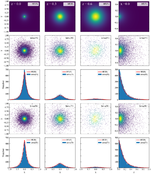
Figure 2: Spatial probability distribution of phosphorylation with $\nu_{a}$=10, $\nu_{d}$=10, $\nu_{l}$=20, and $D_{K}$=0.02 [35, 36, 37, 38] from $10^{7}$ stochastic simulations in CaM scenario. The panels in the first row are for results of phosphorylation events (Pi) in the mean field ansatz (MF). The panels in the second and fourth rows are for the simulation (Simu) results of phosphorylation events (Pi) and trajectories (Tr), respectively. And comparisons between simulation and mean field ansatz are given in third and fifth rows. The color of the scattering points is determined by Gaussian kernel density estimation. The first three columns are for slices at $z=0.0$, 0.3, and 0.6, with thickness $\delta z=0.01$, and the last column is for $x=0$ with $\delta x=0.01$.

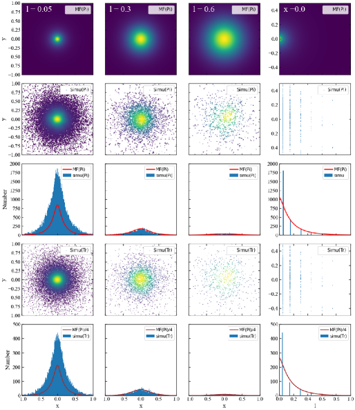
Figure 3: Spatial probability distribution of phosphorylation with $\nu_{a}$=10, $\nu_{d}$=10, $\nu_{l}$=20, $\nu_{b}=\nu_{u}=1$, and $D_{K}$=0.02 [35, 36, 37, 38] from $2\times 10^{5}$ stochastic simulations in PKC scenario. The first three columns are for distances at $l=0.05$, 0.3, and 0.6, with thickness $\delta z=0.01$, and the last column is for $x=0$ with $\delta x=0.01$. Other notations are analogous to those in Fig. 2.

In the first row of Fig. 2, the distribution with mean field (MF) ansatz in Eq. (15) is presented. At small $z$, the phosphorylation concentrates at entrance. When deviating from ER, phosphorylation events distribute in a larger region. In the second and fourth rows, we present simulation results for both phosphorylation events and trajectories. In order to determine event distribution at $z$, we select events (Pi) at position ${\bm{\xi}}$ or trajectories (Tr) at mean position $\hat{\bm{\xi}}$ which are in a range form $z-\delta z/2$ to $z+\delta z/2$. The simulation results exhibit the same picture as the MF ansatz. To give a more obvious comparison, we present the results accumulated at $x$ direction in the third and fifth rows. The MF results are given by $\hat{n}({\bm{r}})\delta z\delta xN$, which is for events not trajectories. The results suggest that the MF results for events fit the simulation as expected. The phosphorylation events concentrates at the entrance, and diminishes rapidly with the increase of $z$ and $x$. It is interesting to observe that the results for trajectories are almost the same as these for events. It suggests that with the current parameters adopted, the number of the events in a trajectory is very small, which ensures the effectiveness of MF ansatz.

Different from CaM scenario, all phosphorylations happen on PM in PKC scenario. In Fig 3, we present the results with different distances, $l=0.05$, $0.3$ and 0.6 between PM and ER. The simulations can not performed when PM and ER overlaps. Here we adopt a small distance $l=0.05$ instead of zero. At small distance, phosphorylations concentrate at center as in CaM scenario. With the increase of distance, the numbers of events and trajectories diminish rapidly. As shown in third and fifth rows, the phosphorylation events and trajectories are relatively more than in CaM scenario. As shown in the last column, the number is about two times large than the line for CaM, that is, $\hat{n}({\bm{r}})\delta xN$. At larger distance, the MF lines in CaM scenario fit the PKC simulation very well as expected. Different from the CaM scenario, the number of trajectories is about four times larger than the number of events. In the last rows, we give the scaled results for MF, it is interesting to see that the lines also fit the simulation results very well at large distances. It suggests that the MF ansatz is still established, though a trajectory contains about 4 events averagely.

3.2. Average position of phosphorylation and buffer effect of kinase

As shown in the above, phosphorylation consternates near ER in CaM scenario, and the number of phosphorylation events in PKC scenario is also much larger at small distance than at large distance. To give a numerical description, here we present average position of phosphorylation in CaM scenario in Fig. 4. Because average positions in $x$ and $y$ directions are zero, we only give $\langle z\rangle$ here. In mean field ansatz, it is defined as

$$\langle z\rangle=\frac{\int_{-\infty}^{\infty}dxdy\int^{\infty}_{0}dz~{}z~{}\hat{n}({\bm{r}})}{\int_{-\infty}^{\infty}dxdy\int^{\infty}_{0}dz~{}\hat{n}({\bm{r}})}=\frac{\lambda_{-}^{2}+\lambda_{-}\lambda_{+}+\lambda_{+}^{2}}{\lambda_{-}^{2}\lambda_{+}+\lambda_{+}\lambda_{+}^{2}}.$$ (17)

In simulation, we will collect all positions of events or mean positions of trajectories $\xi_{zk}$ and the average position $\langle z\rangle=\sum_{k=1}^{m}\xi_{zk}/m$ with $m$ is the total number of events or trajectories.

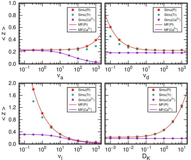
Figure 4: Average positions of phosphorylation and free Ca²⁺ in CaM scenario. The results are obtained by varying one of the parameters, $\nu_{a}$=10, $\nu_{d}$=10, $\nu_{l}$=20, and $D_{K}$=0.02.

With the parameters adopted in previous subsection, the average $\langle z\rangle$ is about 0.2, which corresponds to about 3 $\mu$m before dimensionless treatment. Such value is consistent with the order of the magnitude of a calcium spark [12]. We also discuss the dependence of $\langle z\rangle$ on the parameters. The values are very stable with a rate of attachment $\nu_{a}<100$, a rate of detachment $\nu_{d}>1$, and a diffusion constant $D_{K}<0.1$. The result is more sensitive to the rate of loosing $\nu_{l}$. With larger $\nu_{a}$ and smaller $\nu_{d}$, the Ca²⁺ will attached into the CaM more quickly and enduringly, which reflects by larger $\langle z\rangle$. The large $D_{K}$ of the kinase also leads to larger $\langle z\rangle$. Such results suggest that the CaM is buffer of Ca²⁺ diffusion as suggested in Refs. [7, 8].

To give the buffer effect of CaM more clearly, we also present the average position of free Ca²⁺ when it attaches to kinase or leaving the system before an attachment as described in Eq. (13). The average position with MF ansatz can be obtained as

$$\langle z\rangle=\frac{\int_{-\infty}^{\infty}dxdy\int^{\infty}_{0}dz~{}z~{}\hat{n}_{0}({\bm{r}})}{\int_{-\infty}^{\infty}dxdy\int^{\infty}_{0}dz~{}\hat{n}_{0}({\bm{r}})}=\frac{1}{\omega}.$$ (18)

The simulation results are also presented and compared. We would like to note that the $\langle z\rangle$ for free Ca²⁺ is only dependent on $\nu_{a}$ and $\nu_{l}$. In the stable region, the buffer effect is relatively small. When the $\langle z\rangle$ increases, the buffer effect of the CaM becomes important, and the phosphorylations will happen at a position far away from the ER, for example, with $\nu_{l}=1$, the average position of phosphorylations is at about 30 $\mu$m while the $\langle z\rangle$ for free Ca²⁺ is only about 5 $\mu$m. Larger $\nu_{a}$ and $D_{K}$, small $\nu_{d}$ and $\nu_{l}$ are beneficial to the buffer function of CaM.

In PKC scenario, the average position of phosphorylation is fixed at the PM. Here, we only give the results for free Ca²⁺ and compare them with CaM results with MF ansatz as shown in Fig. 5.

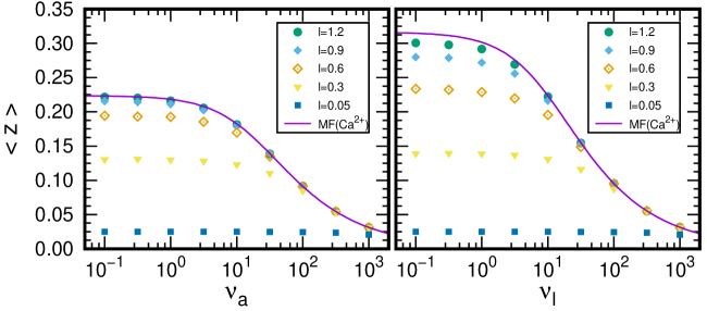
Figure 5: Average position of free Ca²⁺ in PKC scenario. The results are obtained by varying one of the parameters, $\nu_{a}$=10, $\nu_{d}$=10, $\nu_{l}$=20, and $D_{K}$=0.02.

Since Ca²⁺ will be reflected by PM and ER, the distance between two membranes will effect the average position for free Ca²⁺. For a large distance $l=1.2$, as expected the effect of PM becomes small, the results are almost the same as the results in CaM scenario with MF ansatz. In such cases, the buffer effect of the PKC is obvious. Phosphorylations happen at PM which distance is about six time larger than the $\langle z\rangle$ for free Ca²⁺ with $\nu_{a}<1$. With decrease of the distance, the $\langle z\rangle$ becomes small due to the suppression of PM. Meantime, the buffer effect of the kinase becomes relatively small too. For example, at a distance $l=0.3$, the $\langle z\rangle$ is about 0.15 with $\nu_{a}<1$. With increase of both $\nu_{a}$ and $\nu_{l}$, Ca²⁺ will be attached or lost quickly, so the buffer effect becomes more important.

3.3. Estimation error of readout position of Ca²⁺

In the above, we present the average position in $z$ direction. In $x$ and $z$ directions, average position is zero. Here we will give the estimation error to describe the distribution of phosphorylation parallel to ER. With the mean field ansatz it is written as

$$\ell^{2} = \frac{\int_{-\infty}^{\infty}dxdy~{}(x^{2}+y^{2})~{}\hat{n}({\bm{r}})}{\int_{-\infty}^{\infty}dxdy~{}\hat{n}({\bm{r}})}$$ (19)

$$= \frac{2e^{\lambda_{-}z}\lambda_{-}^{3}(1+\lambda_{+}z)-2e^{\lambda_{+}z}\lambda_{+}^{3}(1+\lambda_{-}z)}{\lambda_{-}^{2}\lambda_{+}^{2}(e^{\lambda_{-}z}\lambda_{-}-e^{\lambda_{+}z}\lambda_{+})}.$$

In simulation, in order to determine estimation error at $z$, we will collect the mean position of a simulation $\hat{\bm{\xi}}$ which satifies $z-\delta z/2<\hat{\xi}_{z}<z+\delta z/2$, with a number $n_{z}$. The number distribution is defined as $\hat{n}(z)={n_{z}}/{(n\delta z)}$ and the estimation error as $\ell^{2}(z)=\sum_{k=1}^{n_{z}}(\hat{\xi}^{2}_{x,k}+\hat{\xi}^{2}_{y,k})/n_{z}$. Here, the number distribution $\hat{n}(z)$ is for the phosphorylation trajectories, not for the phosphorylation events.

We present CaM results for the estimation error in Fig. 6. Dependence of parameters and comparison between MF and simulation results are also presented.

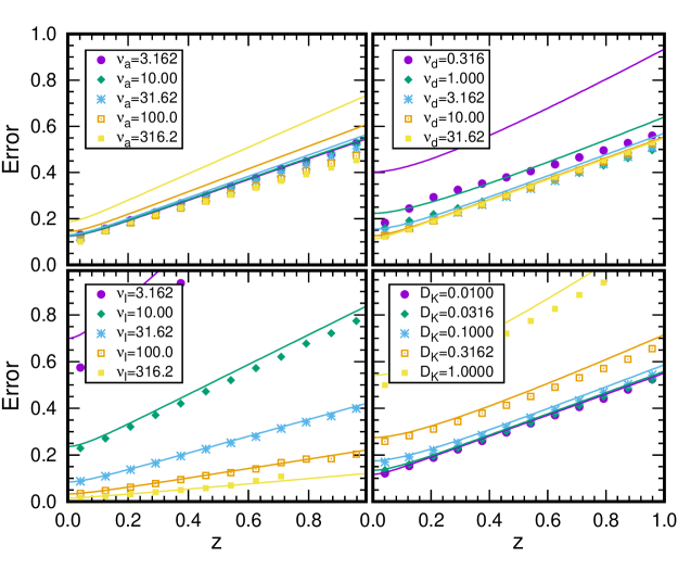
Figure 6: The variation of estimation error against distance with different parameters from $10^{8}$ stochastic simulations in CaM scenario. The results are obtained by varying one of the parameters, $\nu_{a}$=10, $\nu_{d}$=10, $\nu_{l}$=20, and $D_{K}$=0.02.

For all cases, estimation error increases with the increasing of $z$. The results are not sensitive to variation of $\nu_{a}$ in a large region from 3 to 300. For $\nu_{a}$ larger than 100, the simulation results begin to deviate from MF results. Dependence on the parameter $\nu_{d}$ is also small, and appears at small value of $\nu_{d}$. The effect of $\nu_{l}$ is quite large from 3 to 300 while the MF and simulation results fit each other when $\nu_{l}$ larger than 10. The estimation error becomes larger with the increasing of diffusion parameter $D_{K}$. Estimation error $\ell^{2}$ is about 0.2 at the $z=0.2$ with parameters we adopted, which corresponding 5 $\mu$m.

In Fig. 7, We present PKC results for the estimation error, and compare it with the analytical results with Eq. (19) in the CaM scenario. The results suggest the PKC simulation fit MF results in CaM scenario at distance $l>0.2$ as expected. Generally speaking, the PKC results exhibit the same picture as the CaM scenario. Besides, estimation error is independent on $\nu_{b}$ and $\nu_{u}$ as expected.

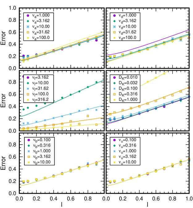
Figure 7: The variation of estimation error against distance with different parameters from $10^{8}$ stochastic simulations in the PKC scenario. Except the varied parameter, $\nu_{a}$=10, $\nu_{d}$=10, $\nu_{l}$=20, $\nu_{b}=1$, $\nu_{u}=1$, and $D_{K}$=0.02.

4. Summary and discussion

Ca²⁺ signal is very important in cell signal transduction, which attracts much attentions from scientific communities in biology, medicine, and physics. For all the research topics of the Ca²⁺ signal, such as calcium spike, calcium wave, and second messenger system, the propagation of Ca²⁺ ion in cytoplasm and its readout are in the most basic level. The study of spatial probability distribution of a Ca²⁺ ion is helpful to understand intracellular Ca²⁺ signal transduction. In the current work, we study three-dimensional Ca²⁺ propagation in two typical CaM and PKC scenarios, and the phosphorylation is adopted to read out Ca²⁺.

In CaM scenario, after released from the calcium channel in ER, Ca²⁺ diffuses in cytoplasm, which corresponds to realistic case, such as a Ca²⁺ event in calcium spike and wave [12]. In such case, Ca²⁺ takes effect near membrane, and effect of other membranes is very small. The result suggests that the probability distribution is only dependent of the radius from entrance. With the parameters chosen [35, 36, 37, 38], the phosphorylation events concentrate at the entrance and diminish exponentially with the radius. At the direction perpendicular to the membrane, the average position is only about several $\mu$m, which is at the same order of magnitude of the width of the calcium spike. The CaM is considered as buffer of the Ca²⁺ propagation in cytoplasm [7, 8]. With the parameters chosen, the buffer effect is not very large. However, there exist many types of CaM which has different properties. The results suggests that the average position in $z$ direction will increase with the increase of the rate of attachment $\nu_{a}$ and diffusion constant $D_{K}$, and decrease of the rate of detachment $\nu_{d}$ and the rate of losing $\nu_{l}$. At the direction parallel to membrane, the average position is zero, error estimation $\ell^{2}$ is calculated to show the coverage of influence of a Ca²⁺ ion. At small $z$, the error estimation is also at an order of several $\mu$m, and it will increase with the increase of $z$ almost linearly. Generally speaking, if Ca²⁺ is read out by phosphorylation, coverage of influence of a Ca²⁺ ion is at an order of $\mu$m. The rates and diffusion constant of the CaM will effect coverage of influence of Ca²⁺ as a buffer. We would like to note that the results in CaM scenario can be applied to all type of membranes, not only the ER considered here.

The PKC scenario is quite different from the CaM scenario. In such scenario, the PKC attached by Ca²⁺ must bind into the PM, which is the important part of the double messenger system. All phosphorylation events happen in PM, and concentrate at zero point. When the distance between ER and PM becomes smaller, the phosphorylation events will decrease very rapidly, especially at small distance. At the same time, the estimation error becomes smaller also. If we recall that the PKC should bind into the PM and activates by the DAG, a small distance between PM and ER, smaller than 1 $\mu$m suggested by current result, will benefit the double message system. In fact, the importance of the ER-PM junction were studied in many works, such as Ca²⁺ influx [39, 40]. The current work suggest that in the ER-PM junction, the efficiency of the double messenger system may be improved greatly.

In summary, the 3-dimensional probability distribution of Ca²⁺ which is read out by phosphorylation in cytoplasm is studied in two scenarios. The results in PKC scenario with two boundaries are found consistent with the results in CaM scenario especially at large distance as suggested by MF ansatz. The coverage of distribution of Ca²⁺ is found at an order of $\mu$m, which is consistent with experimental observed calcium spike and wave. Our results also suggest that the double messenger system may occurs in the ER-PM junction to acquire great efficiency.

References

- [1] D. E. Clapham, Calcium Signaling, Cell 131, 1047 (2017).
- [2] M. J. Berridge, M. D. Bootman, and P. Lipp, Calcium-a life and death signal, Nature 395, 645 (1998).
- [3] M. Berridge, The Inositol Trisphosphate/Calcium Signaling Pathway in Health and Disease, Physiol. Rev. 96, 1261 (2016).
- [4] M. J. Berridge, Rapid accumulation of inositol trisphosphate reveals that agonists hydrolyse polyphosphoinositides instead of phosphatidylinositol, Biochem. J. 212, 849 (1983).
- [5] H. Streb, R. F. Irvine, M. J. Berridge, and I. Schulz, Release of Cd+from a nonmitochondrial store in pancreatic cells by inositol 1,4, 5-trisphosphate, Nature 306, 67 (1983).
- [6] W. Cheung, Calmodulin plays a pivotal role in cellular regulation, Science 207, 19 (1980).
- [7] Jiri Palecek, Mario B. Lips and Bernhard U. Keller, Calcium dynamics and buffering in motoneurones of the mouse spinal cord, Journal of Physiology 520, 485 (1999).
- [8] Linu M. John, Monica Mosquera-Caro, Patricia Camacho and James D. Lechleiter, Control of IP3-mediated Ca2+ puffs in Xenopus laevis oocytes by the Ca2+-binding protein parvalbumin, Journal of Physiology 535, 3 (2001).
- [9] Dongki Yang, Jaehong Kim, Emerging role of transient receptor potential (TRP) channels in cancer progression, BMB Rep. 53, 125 (2020).
- [10] L. F. Jaffe, Classes and mechanisms of calcium waves, Cell Calcium 14, 736 (1993).
- [11] C. Wei, X. Wang, M. Chen, K. Ouyang, L. S. Song, H. Cheng, Calcium flickers steer cell migration, Nature 457, 901 (2009).
- [12] Heping Cheng and W. J. Lederer, Calcium Sparks, Physiological Reviews 88, 1491 (2008).
- [13] J. W. Dani, A. Chernjavsky, S. J. Smith, Neuronal activity triggers calcium waves in hippocampal astrocyte networks, Neuron 8, 429 (1992).
- [14] D S. Bush, Calcium regulation in plant cells and its role in signaling, Annu Rev Plant Physiol Plant Mol Biol 46, 95 (1995).
- [15] T. Yamashita, H. Amano, N. Harada, Z. L. Su, T. Kumazawa, Y. Tsunoda, Y. Tashiro, Calcium distribution and mobilization during depolarization in single cochlear hair cells: Imaging Microscopy and Fura-2, Acta Otolaryngol 109, 256 (1990).
- [16] Domald MO’Malley, Sidney Wang, Visualization of calcium activity in nerve cells, IEEE Computer Graphics and Applications 15, 55 (1995).
- [17] T. Oshima, K. Ikeda, M. Furukawa, N. Ueda, H. Suzuki, T. Takasaka, Distribution of Ca2+ Channels on Cochlear Outer Hair Cells Revealed by Fluorescent Dihydropyridines, Am J Physiol 271, C944 (1996).
- [18] A. Miyawaki, J. Llopis, R. Heim, et al, Fluorescent indicators for Ca2+ based on green fluorescent proteins and calmodulin. Nature 388, 882 (1997).
- [19] M. Schäferling, The Art of Fluorescence Imaging with Chemical Sensors, Angew. Chem. Int. Ed. 51, 3532 (2012).
- [20] H. Cheng, W. J. Lederer, M. B. Cannell, Calcium sparks: Elementary events underlying excitation-contraction coupling in heart muscle, Science 262, 740 (1993).
- [21] H. Cheng, M. R. Lederer, W. J. Lederer, M. B. Cannell, Calcium sparks and [Ca2+]i waves in cardiac myocytes, Am J Physiol 270, C148 (1996).
- [22] Jin Lu and Jinghong Li. Label-Free Imaging of Dynamic and Transient Calcium Signaling in Single Cells, Angew. Chem. Int. Ed. 54, 13576 (2-15).
- [23] S. Rüdiger, J. Shuai, and I. Sokolov, I, Law of Mass Action, Detailed Balance, and the Modeling of Calcium Puffs, Physical Review Letters, 105, 048103 (2010).
- [24] H. Qi, Y. D. Huang, S. Rüdiger, and J. W. Shuai, Frequency and Relative Prevalence of Calcium Blips and Puffs in a Model of Small IP3R Clusters. Biophysical Journal 106, 2353 (2014)
- [25] W. C. Tan, C. Q. Fu, C. J. Fu, W. J. Xie, H. P. Cheng, An anomalous subdiffusion model for calcium spark in cardiac myocytes, Appl Phys Lett 91, 183901 (2007).
- [26] V. H. Wasnik, P. Lipp, and K. Kruse, Positional Information Readout in Ca2+ Signaling, Phys. Rev. Lett. 123, 058102 (2019).
- [27] V. H. Wasnik, P. Lipp, and K. Kruse, Accuracy of position determination in Ca2+ signaling, Phys. Rev. E 100, 022401 (2019).
- [28] Serdar Kuyucak, Olaf Sparre Andersen and Shin-Ho Chung, Models of permeation in ion channels, Rep. Prog. Phys. 64, 1427 (2001).
- [29] S. Chandrasekhar, Stochastic Problems in Physics and Astronomy, Reviews of Modern Physics, 43, 1 (1943).
- [30] B. Hille, Ionic Channels of Excitable Membranes, 2nd edn (Sunderland, MA: Sinauer Associates, 1992)
- [31] J. Crank, The Mathematics of Diffusion (Oxford: Oxford University Press, 1975)
- [32] D. T. Gillespie, Exact Stochastic Simulation of Coupled Chemical Reactions, The Journal of Physical Chemistry 81, 25 (1977).
- [33] R. Erban and S. J. Chapman, Stochastic modelling of reaction-diffusion processes: Algorithms for bimolecular reactions, Phys. Biol. 4, 16 (2007).
- [34] S. S. Andrews and D. Bray, Stochastic simulation of chemical reactions with spatial resolution and single molecule detail, Phys. Biol. 1, 137 (2004).
- [35] E. A. Nalefski, A. C. Newton, Membrane binding kinetics of protein kinase C betaII mediated by the C2 domain, Biochemistry 40, 13216 (2001).
- [36] G. D. Smith, J. E. Keizer, M. D. Stern, W. J. Lederer, and H. Cheng, Detection in Cardiac Myocytes, Biophys. J. 75, 15 (1998).
- [37] B. S. Donahue and R. F. Abercrombie, Free diffusion coefficient of ionic calcium in cytoplasm, Cell Calcium 8, 437 (1987).
- [38] M. Schaefer, N, Albrecht, T. Hofmann, T. Gudermann, G. Schultz, Diffusion-limited translocation mechanism of protein kinase C isotypes, FASEB J 15, 1634 (2001).
- [39] J. Jing, L. He, A. Sun, et al., Proteomic mapping of ER-PM junctions identifies STIMATE as a regulator of Ca2+ influx, Nature Cell Biology, 17, 1339 (2015).
- [40] M. Prakriya, R. S. Lewis, Store-Operated Calcium Channels, Physiological Reviews 95, 1383 (2015).