Optimal Number of Faces for Fast Self-Folding Kirigami

Abstract

We study the spontaneous folding of a 2D template of microscopic panels into a 3D pyramid, driven by thermal fluctuations. Combining numerical simulations and analytical calculations, we find that the total folding time is a non-monotonic function of the number of faces, with a minimum for five faces. The motion of each face is consistent with a Brownian process and folding occurs through a sequence of irreversible binding events that close edges between pairs of faces. The first edge closing is well-described by a first-passage process in 2D, with a characteristic time that decays with the number of faces. By contrast, the subsequent edge closings are all first-passage processes in 1D and so the time of the last one grows logarithmically with the number of faces. It is the interplay between these two different sets of events that explains the non-monotonic behavior. Possible implications in the self-folding of more complex structures are discussed.

Kirigami is the art of cutting two-dimensional templates and fold them into three-dimensional structures. Nowadays, there is a growing interest on extending this ancient idea to design materials that fold spontaneously into targeted 3D structures. The driving mechanism depends on the lengthscale. At the macroscale, folding is driven by energy minimization (e.g. stress relaxation), and thus the folding pathway is deterministic Shenoy and Gracias (2012); Liu et al. (2012); Erb et al. (2013); Castle et al. (2014); Sussman et al. (2015); Dudte et al. (2016); Liu et al. (2016, 2017); Paulsen (2019); Dieleman et al. (2020); Santangelo (2020); Siéfert et al. (2019). By contrast, at the microscale, since folding occurs usually in suspension, the fluctuations in the fluid-structure interaction dominate and folding is stochastic Pandey et al. (2011); Dodd et al. (2018). This challenges the use of Kirigami at the microscale as, for example, in encapsulation, drug delivery, and soft robotics Fernandes and Gracias (2012); Shim et al. (2012); Filippousi et al. (2013); Felton et al. (2014).

To design self-folding Kirigami, one first needs to identify what are the two-dimensional templates (nets) that fold into the desired structure. For shell-like structures of rigid panels connected by edges, these nets are obtained by edge unfolding, i.e., by cutting edges and opening the structure Demaine and O’Rourke (2007). In principle, different nets can fold into the same three-dimensional structure. However, recent experiments and numerical simulations show that the stochastic nature of folding might lead to misfolding. By performing independent samples, they found that the probability for a given net to fold into the desired structure (yield) strongly depends on the topology of the net and experimental conditions Azam et al. (2009); Pandey et al. (2011); Araújo et al. (2018); Dodd et al. (2018). Thus, the focus has been on identifying what are the optimal nets that maximize the yield Pandey et al. (2011); Araújo et al. (2018). But, what about the folding time? For practical applications, it is not only critical to reduce misfolding but also to guarantee that folding occurs in due time. Here, we address this question. To focus on the folding time, we consider as a prototype the spontaneous folding of a pyramid, where misfolding is not possible.

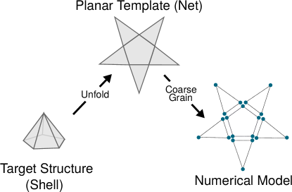
Figure 1: Unfolding process and model. We consider pyramids (left) of one base and $N$ lateral faces ($N=5$ in the figure). The 2D template of microscopic panels (center) is obtained by cutting the edges between the lateral faces and unfolding the faces. To simulate the folding dynamics, we developed a coarse-grained numerical model where each face is described as a rigid body of three particles (right) at the vertices. The base is described by $N$ particles at the vertices. The interaction between particles is considered pairwise and attractive. To suppress misfolding, the base is pinned to a flat substrate and the lateral faces can only fold in one side. 

Let us consider a pyramid with $N$ lateral faces (see Fig. 1). The 2D net is a $N$-pointed star, obtained by cutting the edges of the lateral faces and unfolding them. To simulate the folding dynamics, as explained in detail in the Supplemental Material SM and summarized in Fig. 1, we performed particle-based simulations. We are interested in the limit where the interaction between faces is short-ranged (contact like) and the edge closing irreversible. Thus, each face is described as a rigid body of three particles at the vertices. The attractive interaction along the edges is modeled by a strong inverted-Gaussian potential between particles. The stochastic trajectories of the faces under thermal fluctuations is obtained by solving the corresponding Langevin equations, where the noise term is parameterize by a rotational diffusion coefficient $D_{0}$ of the lateral faces. To suppress misfolding, we pinned the base of the pyramid to a substrate and so the faces can only fold in one side (see Supplemental Material SM for further details).

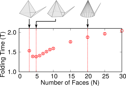
Figure 2: Non-monotonic dependence of the folding time on the number of lateral faces. Folding time as a function of the number of lateral faces ($N$), defined as the total time necessary for all faces to fold into a pyramid. Time is in units of Brownian time, i.e., the average time for a non-interacting face to diffuse over an angular region of size $\pi$. Results are obtained numerically by averaging over $2\times 10^{3}$ independent samples, starting from a flat template. 

We performed independent simulations for different numbers of lateral faces $N$, starting from a flat (2D) configuration and running until the final pyramid is obtained. As shown in Fig. 2, we find that, the total folding time $T$ is a non-monotonic function of the number of faces $N$, with an optimal time for five faces. To characterize the dynamics, we define $\theta_{i}$ as the angle between the face $i$ and the substrate (see scheme in the top of Fig. 3). Since the motion is constrained by the substrate, $\theta_{i}\in\left[0,\pi\right]$.

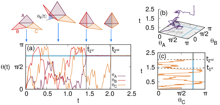
Figure 3: Self-folding of a pyramid of $N=3$ lateral faces. (a) Time dependence of the angle $\theta_{i}$ of each face $i$ with the flat substrate (see scheme). Since the base of the pyramid is pinned and the faces can only move in one side, $\theta_{i}\in\left[0,\pi\right]$. Results are for one sample, starting from a flat template ($\theta_{i}(0)=0$). The statistics of $\theta_{i}$ is consistent with a Brownian process with reflective walls at $\theta_{i}=0$ and $\theta_{i}=\pi$ (see Supplemental Material SM ) and folding occurs through a sequence of edge closings. For the first edge closing, two faces need to be at $\theta^{*}=3\pi/4\pm\Delta$ (region in blue) at the same time, where $\Delta\approx\pi/180$. In the example, this occurs for faces $A$ and $B$ at time $t_{1^{\mathrm{st}}}$. (b) If we assume no interaction between $A$ and $B$ outside the blue region, the first edge closing can be mapped into a 2D Brownian process, with coordinates $\theta_{A}$ and $\theta_{B}$ and a trap in a region where both $\theta_{i}=\theta^{*}$. $t_{1^{\mathrm{st}}}$ is then the first-passage time. (c) After the first edge closing, the third face $C$, performs a 1D Brownian motion until it hits $\theta^{*}$. In the example, this occurs at $t_{2^{\mathrm{nd}}}$. As in Fig. 2, time is rescaled by Brownian time. 

.

As an example, we consider now the folding of a pyramid of three lateral faces ($N=3$). The time dependence of the three angles is shown in Fig. 3(a). Due to thermal fluctuation, each face jiggles around until the first two faces ($A$ and $B$ in the figure) meet at time $t_{1^{\mathrm{st}}}$ and bind irreversibly, closing the edge between them. The third face ($C$) also binds to the first two at a later time $t_{2^{\mathrm{nd}}}$. Thus, folding occurs through a sequence of irreversible edge closings. Below, we discuss the first and subsequent edge closings independently.

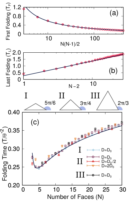
Figure 4: Dependence on the number of lateral faces. (a) Time of first edge closing ($T_{F}$) as a function of $N(N-2)/2$, where $N$ is the number of lateral faces. The first edge closing occurs when two faces have $\theta=\theta^{*}=3\pi/4\pm\Delta$, where $\Delta\approx\pi/180$. $T_{F}$ decreases with $N$. The solid line is given by $T_{F}=\tau_{F}/\ln(N(N-1)/2)+\tau_{F0}$, where $\tau_{F}=1.57\pm 0.02$ and $\tau_{F_{0}}=-0.097\pm 0.006$ are fitting parameters obtained by the least square fit of the simulation data. This expression corresponds to a first-passage time of a 2D Brownian process (see details in the text). (b) Last-edge-closing time as a function of $N-2$. After the first edge closing, $N-2$ faces remain that fold sequentially. $T_{L}$ is given by the slowest of ($N-2$) 1D first-passage events. The solid line is given by $T_{L}=\tau_{L}\ln(N-2)+\gamma\tau_{L}$, with $\tau_{L}=4{\theta^{*}}^{2}/D_{0}\pi^{2}$ and $\gamma$ the Euler-Mascheroni constant. $D_{0}$ is the angular diffusion coefficient of reference (see Supplemental Material SM ). (c) Data collapse for the folding time, in units of Brownian time, rescaled by the square of the folding angle $(\theta^{*})^{2}$, as a function of the number of faces $N$ for different values of $\theta^{*}=\{3\pi/4,2\pi/3,5\pi/6\}$ and $D=\{D_{0},D_{0}/2,2D_{0}\}$. Results are averages over $2\times 10^{3}$ independent samples. 

As shown in the Supplemental Material SM , the statistics of the three time series $\theta_{i}(t)$ in Fig. 3 is consistent with a 1D Brownian process with reflective boundaries at $\theta_{i}=0$ and $\theta_{i}=\pi$. The short-ranged (attractive) interaction between faces is only effective in a small region of the angular space, $\theta^{*}=3\pi/4\pm\Delta$, with $\Delta\approx\pi/180$ as estimated from the properties of the potential (see Supplemental Material SM ). For the first edge closing to occur, the angle of two faces need to be at $\theta^{*}$ at the same time and, once there, they get trapped. Thus, if we map the motion of each pair of faces $j$ and $k$ into a 2D Brownian process, with coordinates $(\theta_{j},\theta_{k})$ and a trap at $(\theta^{*},\theta^{*})$, the edge closing between $j$ and $k$ occurs when the corresponding 2D Brownian process hits the trap (see Fig. 3(b)). In the general case of $N$ lateral faces, since there are $N(N-1)/2$ possible pairs of faces, the time of the first edge closing is the fastest of $N(N-1)/2$ first-passage processes.

To estimate the average time $T_{F}$ of the first edge closing for a pyramid of $N$ lateral faces, we define $g(t)$ as the first-passage time distribution of a 2D Brownian process. There are $N(N-1)/2$ pairs of faces and so the same number of competing Brownian processes. The first edge closing is the fastest of all possible ones and thus $T_{F}=min\{t_{1},t_{2},t_{3}...t_{N(N-1)/2}\}$, where $t_{i}$ are random values following the distribution $g(t)$. If we neglect any correlations between the motion of the different faces, from the theory of order statistics Arnold et al. (1992), we estimate that,

$$T_{F}(N)=\frac{N(N-1)}{2}\int_{0}^{\infty}{tg(t)\left[\int_{t}^{\infty}g(t^{\prime})dt^{\prime}\right]^{\frac{N(N-1)}{2}-1}dt}\ \ ,$$ (1)

where the term with the square brackets corresponds to the probability that, provided that a first-passage process occurs at time $t$, all the remaining $N(N-1)/2-1$ occur at a later time. $g(t)$ depends on the geometry and initial conditions Yuste and Lindenberg (1996); Weiss et al. (1983); Holcman and Schuss (2014); Singer et al. (2006); Yuste (1997). For a set of $N(N-1)/2$ Brownian processes Weiss et al. (1983); Basnayake et al. (2019) starting at the origin ($\theta_{i}(0)=0$),

$$T_{F}(N)\sim 1/\ln\left(\frac{N(N-1)}{2}\right).$$ (2)

So, the time of the first edge closing should decrease with the number of possible pairs. Figure 4(a) shows $T_{F}$ in units of Brownian time (see figure caption), for different numbers of lateral faces, obtained numerically by averaging over $10^{4}$ samples. The solid line is given by $T_{F}=\tau_{F}/\ln\left(N(N-1)/2\right)+\tau_{F_{0}}$, where $\tau_{F}=1.57\pm 0.02$ and $\tau_{F_{0}}=-0.097\pm 0.006$ are obtained by fitting the simulation data. Clearly, the decrease in $T_{F}$ with the number of faces is well described by Eq. (2).

The dynamics of the subsequent edge closings is fundamentally different. While for the first edge closing, two faces need to meet at a particular angular $\theta^{*}$, the remaining faces will close edges one-by-one as soon as they reach $\theta^{*}$. The folding is complete when all faces reach this value. Thus, each of the subsequent ($N-2$) edge closings is a 1D first-passage process (see Fig. 3(c)). We define $T$ as the total folding time and $T_{L}=T-T_{F}$ as the time from the first to the last edge closing. Each free face $i$ binds when $\theta_{i}(T_{F}+t)=\theta^{*}$ (with $t\geq 0$) for the first time. To estimate $T_{L}$, we assume that $\theta_{i}(T_{F})<\theta^{*}$ for all $i$ and that $\theta_{i}(T_{F}+t)$ is well described by a 1D Brownian process, with one reflective boundary at $\theta_{i}=0$ and a trap at $\theta^{*}$. $T_{L}$ is then the slowest of the ($N-2$) 1D first-passage processes. Thus,

$$T_{L}(N)=(N-2)\int_{0}^{\infty}{tf(t)\left[1-\int_{t}^{\infty}f(t^{\prime})dt^{\prime}\right]^{(N-2)-1}dt},$$ (3)

where $f(t)$ is the 1D first-passage time distribution and the term with square brackets is the probability that, provided that a first-passage process occurs at time $t$, all the remaining ones were faster. Assuming that $\theta_{i}(T_{F})$ is uniformly distributed in $\left[0,\theta^{*}\right]$, the first-passage time distribution is $f(t)\approx e^{-t/\tau_{L}}$, with $\tau_{L}=4{\theta^{*}}^{2}/D_{0}\pi^{2}$ Redner (2001), where $D_{0}$ is the diffusion coefficient of the Brownian process. This gives,

$$T_{L}(N)=\tau_{L}\sum_{i=1}^{N-2}\frac{1}{i},$$ (4)

and thus, $T_{L}(N)\approx\tau_{L}\left[\ln(N-2)+\gamma\right]$, where $\gamma$ is the Euler-Mascheroni constant. Figure 4(b) depicts $T_{L}$ obtained numerically for different $N$. The numerical data is consistent with Eq. (4) (solid line).

The dependence on the number of lateral faces $N$ of $T_{F}$ and $T_{L}$ is significantly different. While $T_{F}$ decreases with $N$, $T_{L}$ grows. The total folding time $T$ is the sum of the two. Thus, for low values of $N$, the total folding time is dominated by the time of the first edge closing, whereas for large $N$ is the last closing that sets the overall timescale. It is the interplay between these two timescales that explains the minimum observed in Fig. 2.

So far, we considered always the same closing angle $\theta^{*}$ and diffusion coefficient $D_{0}$. Since the motion of the faces is diffusive, all timescales should scale with $\tau={\theta^{*}}^{2}/2D_{0}$, which is the average time for a non-interacting 1D Brownian process to diffuse in an angular region of size $\theta^{*}$. Figure 4(c) shows the folding time obtained numerically for different values of $\theta^{*}=\{3\pi/4,2\pi/3,5\pi/6\}$ and $D=\{D_{0},D_{0}/2,2D_{0}\}$. A data collapse is obtained when time, initially in units of Brownian time is rescaled by $(\theta^{*})^{2}$. The solid line is the sum of the solid lines for $T_{F}$ and $T_{L}$ in Figs. 4(a) and (b), respectively, and describes quantitatively the dependence on the number of lateral faces.

Conclusions. Under thermal fluctuation, a $N$-pointed star template of rigid panels and flexible hinges folds into a 3D pyramid of $N$ lateral faces. Folding occurs through a sequence of edge closings, but the nature of the first and subsequent edge closings is significantly different. For the first edge closing, two jiggling faces need to meet at a particular angle, whereas for the subsequent edge closings, only one face needs to reach that angle. We hypothesized that the first edge closing can be mapped into a first-passage event of a 2D Brownian process Holcman and Schuss (2015); Schuss et al. (2007); Singer et al. (2006); Holcman and Schuss (2014), obtaining an expression for the corresponding time. This expression predicts that the time for the first edge closing decreases with $N$, what describes quantitatively the numerical data. By contrast, to estimate the time for the subsequent edge closing, we mapped them into a set of first-passage events in 1D and derived the time for the slowest of them all. We predict that this time should rather grow logarithmically with $(N-2)$, which is also observed numerically. Since the total folding time is the sum of the two times, a non-monotonic dependence on $N$ is found.

Spontaneous folding at the microscale is an intricate process that might depend on the physical properties of the structure, fluid-structure interactions, and thermostat temperature Pandey et al. (2011); Dodd et al. (2018); Araújo et al. (2018). Nevertheless, our approach shows that, by mapping folding into a set of competing Brownian processes and binding events, one can predict accurately the relevant time scales. For simplicity, we considered a pyramid, a structure with equivalent folding panels. In general, the template for a given polyhedral structures has different types of panels. They differ not only in shape and size, but also in their position relative to the panel of reference (e.g. base). To extend our framework to those structures, it is critical to consider that folding evolve through a hierarchy of edge closing events that depend on the kinetic pathway of folding.

Acknowledgments. We acknowledge financial support from the Portuguese Foundation for Science and Technology (FCT) under Contracts nos. PTDC/FIS-MAC/28146/2017 (LISBOA-01-0145-FEDER-028146), UIDB/00618/2020, UIDP/00618/2020, and CEECIND/00586/2017.

References

- Shenoy and Gracias (2012) V. B. Shenoy and D. H. Gracias, “Self-folding thin-film materials: From nanopolyhedra to graphene origami,” MRS Bull. 37, 847–854 (2012).
- Liu et al. (2012) Y. Liu, J. K. Boyles, J. Genzer, and M. D. Dickey, “Self-folding of polymer sheets using local light absorption,” Soft Matter 8, 1764–1769 (2012).
- Erb et al. (2013) R. M. Erb, J. S. Sander, R. Grisch, and A. R. Studart, “Self-shaping composites with programmable bioinspired microstructures,” Nat. Commun. 4, 1–8 (2013).
- Castle et al. (2014) T. Castle, Y. Cho, X. Gong, E. Jung, D. M. Sussman, S. Yang, and R. D. Kamien, “Making the cut: Lattice kirigami rules,” Phys. Rev. Lett. 113, 245502 (2014).
- Sussman et al. (2015) D. M. Sussman, Y. Cho, T. Castle, X. Gong, E. Jung, S. Yang, and R. D. Kamien, “Algorithmic lattice kirigami: A route to pluripotent materials,” Proc. Natl. Acad. Sci. U.S.A. 112, 7449–7453 (2015).
- Dudte et al. (2016) L. H. Dudte, E. Vouga, T. Tachi, and L. Mahadevan, “Programming curvature using origami tessellations,” Nat. Mater. 15, 583–588 (2016).
- Liu et al. (2016) Y. Liu, J. Genzer, and M. D. Dickey, ““2d or not 2d”: Shape-programming polymer sheets,” Prog. Polym. Sci. 52, 79–106 (2016).
- Liu et al. (2017) Y. Liu, B. Shaw, M.D. Dickey, and J. Genzer, “Sequential self-folding of polymer sheets,” Sci. Adv. 3, e1602417 (2017).
- Paulsen (2019) J. D. Paulsen, “Wrapping liquids, solids, and gases in thin sheets,” Annu. Rev. Condens. Matter Phys. 10, 431–450 (2019).
- Dieleman et al. (2020) P. Dieleman, N. Vasmel, S. Waitukaitis, and M. van Hecke, “Jigsaw puzzle design of pluripotent origami,” Nat. Phys. 16, 63–68 (2020).
- Santangelo (2020) C. Santangelo, “A fold strategy,” Nat. Phys. 16, 7–8 (2020).
- Siéfert et al. (2019) E. Siéfert, E. Reyssat, J. Bico, and B. Roman, “Bio-inspired pneumatic shape-morphing elastomers,” Nat. Mater. 18, 24–28 (2019).
- Pandey et al. (2011) S. Pandey, M. Ewing, A. Kunas, N. Nguyen, D. H. Gracias, and G. Menon, “Algorithmic design of self-folding polyhedra,” Proc. Natl. Acad. Sci. U.S.A. 108, 19885–19890 (2011).
- Dodd et al. (2018) P. M. Dodd, P. F. Damasceno, and S. C. Glotzer, “Universal folding pathways of polyhedron nets,” Proc. Natl. Acad. Sci. U.S.A. 115, E6690–E6696 (2018).
- Fernandes and Gracias (2012) R. Fernandes and D. H. Gracias, “Self-folding polymeric containers for encapsulation and delivery of drugs,” Adv. Drug Deliv. Rev. 64, 1579–1589 (2012).
- Shim et al. (2012) J. Shim, C. Perdigou, E. R. Chen, K. Bertoldi, and P. M. Reis, “Buckling-induced encapsulation of structured elastic shells under pressure,” Proc. Natl. Acad. Sci. U.S.A. 109, 5978–5983 (2012).
- Filippousi et al. (2013) M. Filippousi, T. Altantzis, G. Stefanou, M. Betsiou, D. N. Bikiaris, M. Angelakeris, E. Pavlidou, D. Zamboulis, and G. van Tendeloo, “Polyhedral iron oxide core–shell nanoparticles in a biodegradable polymeric matrix: preparation, characterization and application in magnetic particle hyperthermia and drug delivery,” RSC Adv. 3, 24367–24377 (2013).
- Felton et al. (2014) S. Felton, M. Tolley, E. Demaine, D. Rus, and R. Wood, “A method for building self-folding machines,” Science 345, 644–646 (2014).
- Demaine and O’Rourke (2007) E. D. Demaine and J. O’Rourke, Geometric folding algorithms: linkages, origami, polyhedra (Cambridge University Press, 2007).
- Azam et al. (2009) A. Azam, T. G. Leong, A. M. Zarafshar, and D. H. Gracias, “Compactness determines the success of cube and octahedron self-assembly,” PLOS ONE 4, e4451 (2009).
- Araújo et al. (2018) N. A. M. Araújo, R. A. da Costa, S. N. Dorogovtsev, and J. F. F. Mendes, “Finding the optimal nets for self-folding kirigami,” Phys. Rev. Lett. 120, 188001 (2018).
- (22) See Supplemental Material at, which includes Refs. .
- Arnold et al. (1992) B. C. Arnold, N. Balakrishnan, and H. N. Nagaraja, A first course in order statistics, Vol. 54 (Siam, 1992).
- Yuste and Lindenberg (1996) S. B. Yuste and K. Lindenberg, “Order statistics for first passage times in one-dimensional diffusion processes,” J. Stat. Phys. 85, 501–512 (1996).
- Weiss et al. (1983) G. H. Weiss, K. E. Shuler, and K. Lindenberg, “Order statistics for first passage times in diffusion processes,” J. Stat. Phys. 31, 255–278 (1983).
- Holcman and Schuss (2014) D. Holcman and Z. Schuss, “The narrow escape problem,” SIAM Rev. 56, 213–257 (2014).
- Singer et al. (2006) A. Singer, Z. Schuss, and D. Holcman, “Narrow escape, part iii: Non-smooth domains and riemann surfaces,” J. Stat. Phys. 122, 491–509 (2006).
- Yuste (1997) S. B. Yuste, “Escape times of j random walkers from a fractal labyrinth,” Phys. Rev. Lett. 79, 3565 (1997).
- Basnayake et al. (2019) K. Basnayake, Z. Schuss, and D. Holcman, “Asymptotic formulas for extreme statistics of escape times in 1, 2 and 3-dimensions,” J. Nonlinear Sci. 29, 461–499 (2019).
- Redner (2001) S. Redner, A guide to first-passage processes (Cambridge University Press, 2001).
- Holcman and Schuss (2015) D. Holcman and Z. Schuss, Stochastic narrow escape in molecular and cellular biology (Springer, New York, 2015).
- Schuss et al. (2007) Z. Schuss, A. Singer, and D. Holcman, “The narrow escape problem for diffusion in cellular microdomains,” Proc. Natl. Acad. Sci. U.S.A. 104, 16098–16103 (2007).