GAS KINEMATICS OF THE MASSIVE PROTOCLUSTER G286.21+0.17 REVEALED BY ALMA

Abstract

We study the gas kinematics and dynamics of the massive protocluster G286.21+0.17 with the Atacama Large Millimeter/submillimeter Array using spectral lines of $\rm C^{18}O$(2-1), $\rm N_{2}D^{+}$(3-2), $\rm DCO^{+}$(3-2) and $\rm DCN$(3-2). On the parsec clump scale, $\rm C^{18}O$ emission appears highly filamentary around the systemic velocity. $\rm N_{2}D^{+}$ and $\rm DCO^{+}$ are more closely associated with the dust continuum. $\rm DCN$ is strongly concentrated towards the protocluster center, where no or only weak detection is seen for $\rm N_{2}D^{+}$ and $\rm DCO^{+}$, possibly due to this region being at a relatively evolved evolutionary stage. Spectra of 76 continuum defined dense cores, typically a few 1000 AU in size, are analysed to measure their centroid velocities and internal velocity dispersions. There are no statistically significant velocity offsets of the cores among the different dense gas tracers. Furthermore, the majority (71%) of the dense cores have subthermal velocity offsets with respect to their surrounding, lower density $\rm C^{18}O$ emitting gas. Within the uncertainties, the dense cores in G286 show internal kinematics that are consistent with being in virial equilibrium. On clumps scales, the core to core velocity dispersion is also similar to that required for virial equilibrium in the protocluster potential. However, the distribution in velocity of the cores is largely composed of two spatially distinct groups, which indicates that the dense molecular gas has not yet relaxed to virial equilibrium, perhaps due to there being recent/continuous infall into the system.

1 Introduction

While it is generally agreed that most stars form in clusters and/or associations rather than in isolation (e.g., Lada & Lada, 2003; Gutermuth et al., 2009; Bressert et al., 2010), there is no consensus for how this comes about. Several fundamental questions about star cluster formation are still debated. For example, is the process initiated by internal processes within a Giant Molecular Cloud (GMC), such as decay of support by supersonic turbulence or magnetic fields, or external processes, such as triggering by cloud-cloud collisions or feedback-induced shock compression (see e.g., Tan, 2015).

Once underway, is cluster formation a fast or a slow process relative to the local freefall time ($t_{\rm ff}$)? Tan et al. (2006) and Nakamura & Li (2007) proposed that formation times are relatively long, i.e., $\sim 10t_{\rm ff}$, especially for those clusters with high ($\gtrsim$ 30%) overall star formation efficiency, since simulations of self-gravitating, turbulent, magnetized gas show low formation efficiency of just $\sim$2% per free-fall time (Krumholz & McKee, 2005; Padoan & Nordlund, 2011). Alternatively, Elmegreen (2007), Hartmann & Burkert (2007) and Hartmann et al. (2012) have argued for cluster formation in just one or a few free-fall times. Another question is: what sets the overall star formation efficiency during cluster formation? The formation timescale and overall efficiency are likely to affect the ability of a cluster to remain gravitationally bound, which on large scales influences global ISM feedback, e.g., concentrated feedback from clusters can create superbubbles (e.g., Krause et al., 2013), and on small scales controls the feedback environments and tidal perturbations of protoplanetary disks (e.g., Adams, 2010).

Star cluster formation is likely to be the result of a complex interaction of numerous physical processes including turbulence, magnetic fields and feedback. From the observational side, measuring the structure and kinematic properties of the dense gas component is needed to provide constraints for different theretical models. Previously, Walsh et al. (2004) found small velocity differences between dense cores and surrounding envelopes for a sample of low-mass cores. Kirk et al. (2007, 2010) surveyed the kinematics of over 150 candidate dense cores in the Perseus molecular cloud with pointed $\rm N_{2}H^{+}$ and $\rm C^{18}O$ observations and found subvirial core to core velocity dispersions in each region. A similar small core velocity dispersion was also found in the Ophiuchus cloud (André et al., 2007). Qian et al. (2012) searched for $\rm{}^{13}CO$ cores in the Taurus molecular cloud and found the core velocity dispersion exhibits a power-law behavior as a function of the apparent separation, similar to Larson’s law for the velocity dispersion of the gas, which suggests the formation of these cores has been influenced by large-scale turbulence.

These observations have generally focused on nearby low-mass star-forming regions. With the unprecedented sensitivity and spatial resolution of ALMA, more light has been shed on massive star forming regions from the “clump” scale (of about a few parsecs) to the “core” scale ($\sim 0.01$ to $0.1\>$pc) (e.g., Beuther et al., 2017; Fontani et al., 2018; Lu et al., 2018). Multiple coherent velocity components from filamentary structures have been reported in some massive Infrared Dark Clouds (IRDCs) (Henshaw et al., 2013, 2014; Sokolov et al., 2018), similar to the structures seen in the nearby Taurus region by Hacar et al. (2013). “Hub-filament” systems have also been reported in some massive star forming regions across a variety of evolutionary stages, perhaps indicating presence of converging flows that channel gas to the junctions where star formation is most active (e.g., Hennemann et al., 2012; Peretto et al., 2014; Lu et al., 2018; Yuan et al., 2018).

However, complete surverys for the dense gas component of massive protoclusters down to the individual core scale, are still rare (e.g., Ohashi et al., 2016; Ginsburg et al., 2017) and a large spatial dynamic range is required to perform a multi-scale kinematics analysis.

Until recently only very few nearby regions were known that were candidates for very young and still forming massive star clusters. One particular promising star-forming clump is G286.21+0.17 (in short G286). It is a massive protocluster associated with the $\eta$ Car giant molecular cloud at a distance of 2.5 $\pm$ 0.3 kpc, in the Carina spiral arm (e.g., Barnes et al., 2010). We performed a core mass function (CMF) study towards this region based on ALMA Cycle 3 observations in Cheng et al. (2018).

Here we present a follow-up study of multiple spectral lines to investigate the gas kinematics and dynamics of G286 from clump to core scales. The paper is organized as follows: in section 2 we describe the observational setup and analysis methods; the results are presented in section 3. We discuss the kinematics and dynamics for parsec-scale filaments and dense cores separately in section 4 and section 5, and then summarize our findings in section 6.

2 Observational Data

2.1 ALMA Observations

Figure 1: Three color image of G286 constructed by combining Spitzer IRAC 3.6 $\mu$m (blue), 8.0 $\mu$m (green), and Herschel PACS 70 $\mu$m (red). Black contours show the 1.3 mm continuum image combining ALMA 12-m and 7-m array data (with a resolution of 1.62″$\times$1.41″). The contour levels are 1$\sigma$ $\times$ (4, 10, 20, 50, 100) with $\sigma$=0.45mJy beam^-1. Grey contours show the 1.3 mm continuum image with only 7-m array data (with a resolution of 7.32″$\times$4.42″, shown in lower left corner). The contour levels are 1$\sigma\times$ (4, 10, 20, 50, 100) with $\sigma$=1.7mJy beam^-1. The position of three filamentary structures are marked in blue text. The G286 field is divided into five strips, as shown by the green rectangles. Each strip is covered with 147 pointings of the 12-m array. The large white ellipse denotes the boundary defined by Mopra HCO⁺(1-0) emission (Barnes et al., 2011), with the major and minor axes equal to twice the FWHM lengths of the 2D gaussian fits to its emission. Two smaller ellipses indicate the approximate boundaries of two sub-regions with distinct radial velocities revealed by multiple gas tracers.

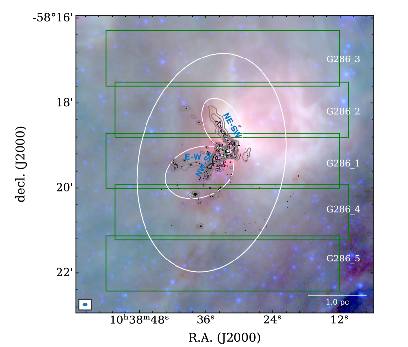
The observations were conducted with ALMA in Cycle 3 (Project ID 2015.1.00357.S, PI: J. C. Tan), during a period from Dec. 2015 to Sept. 2016. More details of the observations can be found in Cheng et al. (2018). In summary, we divided the region into five strips, denoted as G286_1, G286_2, G286_3, G286_4 and G286_5, each about $1\arcmin\>$ wide and $5.3\arcmin\>$ long and containing 147 pointings of the 12-m array (see Figure 1). The position of field center is R.A.=10:38:33, decl.=-58:19:22. We employed the compact configuration C36-1 to recover scales between 1.5″ and 11.0″. This is complemented by observations with the ACA array, which probes scales up to 18.6″. Total power (TP) observations were also carried out to recover the total flux (of line emission), which gives a resolution of about 30″.

During the observations, we set the central frequency of the correlator sidebands to be the rest frequency of the $\rm{N_{2}D}^{+}$(3-2) line at $231.32\>$GHz for SPW0, and the $\rm{C^{18}O}$(2-1) line at $219.56\>$GHz for SPW2, with a velocity resolution of 0.046 and 0.048 km s^-1, respectively. The second baseband SPW1 was set to $231.00\>$GHz, i.e., 1.30 mm, to observe the continuum with a total bandwidth of $2.0\>$GHz, which also covers CO(2-1) with a velocity resolution of 0.64 km s^-1. The frequency coverage for SPW3 ranges from 215.85 to $217.54\>$GHz to observe DCN(3-2), DCO⁺(3-2), SiO($v=0$)(5-4) and $\rm{CH_{3}OH}(5_{1,4}-4_{2,2})$. This paper will focus mostly on dense gas tracers $\rm C^{18}O$, $\rm N_{2}D^{+}$, $\rm DCO^{+}$ and $\rm DCN$.

The raw data were calibrated with the data reduction pipeline using Casa 4.7.0. The continuum visibility data were constructed with all line-free channels. We performed imaging with tclean task in Casa and during cleaning we combined data for all five strips to generate a final mosaic map. Two sets of images were produced for different aspects of the analysis, one including the TP and 7-m array data and one combining TP, 7-m and 12-m data. The 7-m array data was imaged using a Briggs weighting scheme with a robust parameter of 0.5, which yields a resolution of $7.32\arcsec\times 4.42\arcsec\>$. For the combined data, we used the same Briggs parameter. In addition, since we have extra $uv$ coverage for part of the data, we also apply a 0.6″  uvtaper to suppress longer baselines, which results in $1.62\arcsec\times 1.41\arcsec\>$ resolution. Both image sets are then feathered with the total power image to correct for the missing large scale structures. Our sensitivity level is about 30 mJy per beam per 0.1 km/s for $\rm{N_{2}D^{+}}$ and $\rm{C^{18}O}$. A sensitivity of 45 mJy per beam per 0.1 km/s is achieved for $\rm DCO^{+}$(3-2), $\rm DCN$(3-2), SiO(5-4) and $\rm CH_{3}OH$$(5_{1,4}-4_{2,2})$.

2.2 Herschel Observations

The FIR dust continuum images of G286 were taken from Herschel Infrared GALactic plane survey (Hi-GAL; Molinari et al., 2010, 2016). The data includes Photodetector Array Camera and Spectrometer (PACS) (70 and 160 $\mu$m) and Spectral and Photometric Imaging REceiver (SPIRE) (250, 350, and 500 $\mu$m) images. We performed pixel by pixel graybody fits to derive the mass surface density ($\Sigma$) of the G286 region, following the procedures in Lim et al. (2016). The background was estimated as the median intensity value between 2 and 4 times the ellipse aperture shown in Figure 1. To better probe the smaller, higher $\Sigma$ structures, we generated a higher-resolution $\Sigma$ map by regridding the $\lambda\sim$160 to 500$\mu$m images to match the 250$\mu$m data (see Lim et al., 2016, for details).

3 General Results

An overview of the observed region and the layout of the ALMA observations is shown in Figure 1. With the large spatial dynamic range of the ALMA dataset, we will present the large scale structures traced with single dish TP observations first, followed by higher resolution 7-m and 12-m array observations.

3.1 Observations with the Total Power (TP) Array

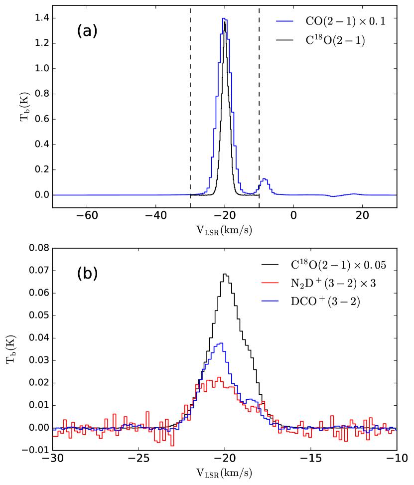
Figure 2a shows the spectra of CO(2-1) and $\rm C^{18}O$(2-1) averaged inside a 2.5′ radius aperture centered on the phase center. The CO(2-1) line has a maximum around the known systemic velocity of about -20 km s^-1. A secondary, much weaker peak is seen around -9 km s^-1. This component is also seen in the Mopra CO(2-1) map, which appears to be a diffuse structure larger than our field of view. We expect that this feature is probably contributed by a foreground or background cloud along line of sight and there is no indication of an interaction between this cloud and G286. Emission from $\rm C^{18}O$(2-1) is only seen from the main $-20$ km s^-1 component.

Figure 2b shows the spectra of the deuterated dense gas tracer $\rm N_{2}D^{+}$(3-2) and $\rm DCO^{+}$(3-2), averaged over the same region, and compared to $\rm C^{18}O$(2-1), zooming-in to the velocity range of the main -20 km s^-1 component. Deuterated species, such as $\rm DCO^{+}$ and $\rm N_{2}D^{+}$ are expected to be tracers of cold, dense gas, including material that is contained in pre-stellar cores (e.g., Crapsi et al., 2005; Bergin & Tafalla, 2007; Kong et al., 2015), and typically optical thin even at the core scale, as found in some examples in IRDCs (Tan et al., 2013). Interestingly, the $\rm C^{18}O$(2-1) line exhibits a main gaussian-like profile with a slight skewness (or second component) to the redshifted side. The spectrum from $\rm DCO^{+}$(3-2) shows a more pronounced double-peaked profile, with one component at about -20.5 km s^-1 and the other at -18.5 km s^-1.

The double-peak profile, i.e., with a stronger blue wing, has also been seen in the $\rm HCO^{+}$(1-0) and $\rm HCO^{+}$(4-3) line in Barnes et al. (2010), with similar central velocities for both peaks. It was interpreted by Barnes et al. (2010) as a canonical inverse P-Cygni profile indicating gravitational infall (Zhou et al., 1993). However, in this picture we would expect a single gaussian profile for optical thin tracers at the self-absorption velocity, in contrast to our $\rm DCO^{+}$(3-2) spectrum. We will return in section 5 to the question of whether the claimed inverse P-Cygni profile in $\rm HCO^{+}$ is really tracing global clump infall or whether it is arising from distinct spatial and kinematic substructures in the protocluster.

To further explore the kinematic structure of the clump, we present the CO(2-1) channel map from $-55.0\>$km s^-1 to 15.0 km s^-1  in Figure 3(a), where we have averaged four velocity channels in each displayed panel. The CO emission is widespread around the systemic velocity (-23 km s^-1 to -17 km s^-1). Bluewards of the line center the emission retains extension towards the southeast and then at the highest blueshifted velocities, e.g., $v\lesssim-45\>$km s^-1, appears more concentrated. The redshifted emission shows more complex structure, including from emission features already mentioned at around $v=-9\>$km s^-1, which may be from an unrelated cloud along the line of sight. However, high velocity ($\Delta v\gtrsim 25\>$km s^-1) redshifted gas is still seen near the phase center. These high velocity features, both blue- and redshifted, are likely to be caused by protostellar outflow activity from within the G286 star-forming clump.

Figure 2: (a) Averaged CO(2-1) and C¹⁸O(2-1) TP spectra extracted over a 2.5′  radius aperture centered on the phase center. Note the flux scale of CO(2-1) has been reduced by a factor of 10. (b) Same as (a) but for $\rm C^{18}O$(2-1), $\rm N_{2}D^{+}$(3-2) and $\rm DCO^{+}$(3-2) in a smaller velocity range from -30 to -10 km s^-1. The flux scale of $\rm C^{18}O$(2-1) is reduced by a factor of 20 and that of $\rm N_{2}D^{+}$(3-2) is increased by a factor of 3 for ease of comparison. Note the $\rm N_{2}D^{+}$(3-2) emission is affected by hyperfine structure, while the $\rm DCO^{+}$(3-2) is not.

Figure 3: (a) Channel maps of TP CO(2-1) emission integrated over every 2.0 km s^-1, as indicated in the upper left of each panel (indicating central velocity of the range), from -55.0 to +15.0 km s^-1. The contour levels are 1 Jy beam^-1 km s^-1$\times$ (1, 5, 10, 20, 40, 80, 200). The red cross in each panel marks the phase center of the observation (R.A.=10:38:33, decl.=-58:19:22). The thick black contour in the lower left panel shows the 4$\sigma$ level of the 7-m continuum emission. (b) Channel maps of TP $\rm C^{18}O$(2-1) emission integrated over every 1.0 km s^-1, with ranges from $-$22.5 to $-$17.5 km s^-1. The contour levels are 1 Jy beam^-1 km s^-1$\times$ (1, 5, 10, 20, 40, 80, 200). The thick black contour in the left panel shows the 4$\sigma$ level of the 7-m continuum emission.

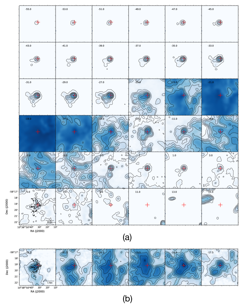
The clump-averaged spectra could be affected by multiple factors including collapse, rotation and outflows. To better resolve the kinematics near the systemic velocity where ¹²CO(2-1) is expected to be mostly optically thick, in Figure 3(b) we show the $\rm C^{18}O$(2-1) channel map from -23.0 km s^-1  to -17.0 km s^-1. This $\rm C^{18}O$ emission at around -20 km s^-1 is moderately elongated in the North-South direction. In the central 2′ region, the $\rm C^{18}O$(2-1) at blueshifted velocities is mostly extended to the southeast, while at the corresponding redshifted velocities, there is a more complex, widespread morphology, including some material at northeastern and southeastern locations.

3.2 Observations of the 7-m and 12-m arrays

Figure 4: Summary figure for the 7-m and 12-m line observations. Columns from left to right show the results of $\rm C^{18}O$(2-1), $\rm N_{2}D^{+}$(3-2), $\rm DCO^{+}$(3-2) and $\rm DCN$(3-2), respectively. From top to bottom, the color scales show the maps of 7-m moment 0, 7-m moment 1, 7-m+12-m moment 0, 7-m+12-m moment 1. The color bar at the right corner indicates the flux scale in Jy beam^-1 for moment 0 maps, and velocity in km s^-1  for moment 1 maps. The black contours illustrates the 1.3 mm continuum emission for comparision, with the first two rows showing 7-m cotinuum image and last two rows 7-m+12-m image.

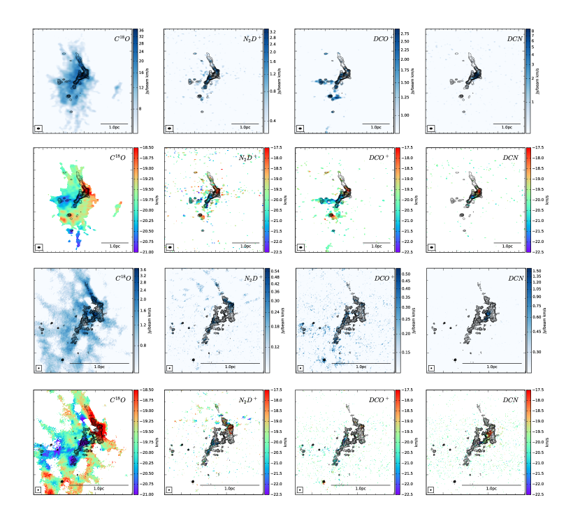
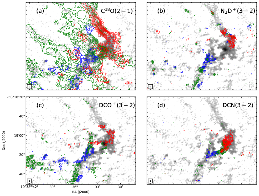
Figure 4 presents summary maps of four spectral lines $\rm C^{18}O$(2-1), $\rm N_{2}D^{+}$(3-2), $\rm DCO^{+}$(3-2) and $\rm DCN$(3-2) from left to right overlaid on 1.3 mm continuum image in black contours. The top two rows show the moment 0 and moment 1 map of the 7-m array images, respectively. As shown in the moment 0 map, $\rm C^{18}O$ traces structures that are more spatially extended than other lines. $\rm N_{2}D^{+}$ and $\rm DCO^{+}$ are more closely associated with the dust continuum, but their distributions are slightly different. $\rm N_{2}D^{+}$ is mainly detected towards the NW-SE filament and the southern part of the NE-SW filament. Note also that not all the regions with strong dust continuum have detections of $\rm N_{2}D^{+}$. In particular, there is a deficiency of $\rm N_{2}D^{+}$ emission towards the central brightest clump. $\rm DCO^{+}$ emission, on the other hand, appears slightly more extended. There is also an E-W filamentary feature to the east of NW-SE filament. This E-W filament is not seen clearly in continuum emission, where we only observe a few cores strung out along the EW direction, but these do appear to be connected by weak diffuse dust emission seen at a 3-$\sigma$ level. Additionally, $\rm DCO^{+}$ is also detected towards a few positions to the south of NW-SE filament. The spatial distribution of $\rm DCN$ emission is dramatically different from $\rm N_{2}D^{+}$ and $\rm DCO^{+}$: it is strongly concentrated towards the clump in the center, where no detection or only weak detection is seen for $\rm N_{2}D^{+}$ and $\rm DCO^{+}$. $\rm DCN$ emission becomes weaker away from the center.

The different morphological distributions of the deuterated species may be due chemical differentiation. In general, $\rm N_{2}D^{+}$ is known as a good tracer of cold ($T\lesssim 20\>$K), dense gas, where $\rm H_{2}D^{+}$ builds up in abundance, but where CO is mostly frozen out on to dust grains (e.g., Fontani et al., 2015). Formation of $\rm DCO^{+}$ requires both $\rm H_{2}D^{+}$ and gas phase CO (e.g., Millar et al., 1989), which requires a temperature $\lesssim$ 30 K but not too cold to cause significant CO freeze-out. On the other hand, the primary DCN formation mechanisms are thought to require $\rm CH_{2}D^{+}$ instead of $\rm H_{2}D^{+}$, which is energetically favorable up to $\sim$80 K (e.g., Millar et al., 1989; Turner, 2001). Additionally, sputtering from grain mantles can also lead to enhancement of DCN abundance in shocked regions (e.g., Busquet et al., 2017). Hence we would generally expect more DCN emssion in relatively later evolutionary stages. The concentrated distribution of DCN, combined with more wide-spread $\rm N_{2}D^{+}$ and $\rm DCO^{+}$ emission, indicates a sceneario that star formation, especially more massive, luminous star formation, has taken place first in the central regions of G286 compared to in the more extended filaments.

The second row of Figure 4 shows the moment 1 map of the 7-m array images. The $\rm C^{18}O$ moment 1 map reveals redshifted emission associated with the NE-SW filament and then continuing to the south of NW-SE filament, while the NW-SE filament and E-W filament are mainly associated with blueshifted gas. Other dense gas tracers show similar velocity patterns as $\rm C^{18}O$, but with the emission mainly detected towards dense continuum clumps. In particular, DCN illustrates the blue-red velocity transition across the central clump in the NW-SE direction.

A zoom-in view of G286 is presented in the third and fourth row of Figure 4, illustrating the moment 0 and moment 1 map of combined 12-m+7-m array image with a resolution of $\sim$ 1.5”. The continuum image reveals a higher level of fragmentation and many well-defined dense cores, with a typical size of a few thousand AU. The E-W filament and part of the NE-SW filament are resolved out in this continuum image. The intensity and velocity distribution of $\rm C^{18}O$ appears more complicated seen in high resolution. Other dense gas tracers like $\rm N_{2}D^{+}$ still have good association with continuum at the core scale, and the velocity pattern is also consistent with that seen in the 7-m image.

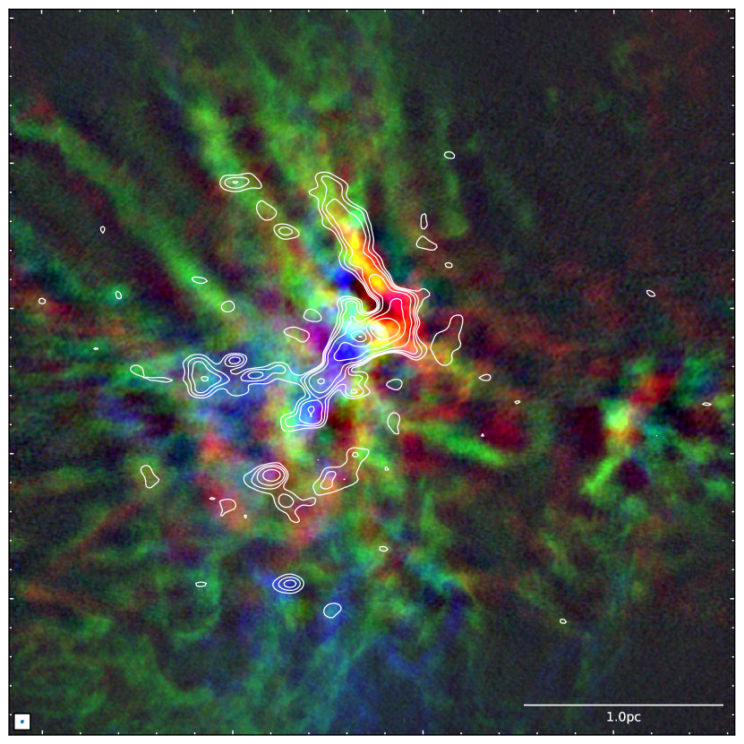
In Figure 5 we present the 12-m + 7-m $\rm C^{18}O$ image with integrated emission in different velocity intervals shown in different colors, i.e., -23.0 to -20.5 km s^-1 in blue, -20.5 to -19.5 km s^-1 in green and -19.5 to -17.0 km s^-1 in red. Besides the velocity structures seen in Figure 4, this plot also reveals highly filamentary $\rm C^{18}O$ features around the systemic velocity. These filaments are more spatially extended than the continuum. While some of this morphology may be affected by artificial sidelobes from imperfect cleaning of the interferometric data, at least some of the $\rm C^{18}O$(2-1) filaments have corresponding detections in the continuum and hence are most likely to be real features.

Figure 5: Three color image constructed with integrated 12-m + 7-m $\rm C^{18}O$(2-1) emission (-23.0 – -20.5 km s^-1  in blue, -20.5 – -19.5 km s^-1  in green and -19.5 – -17.0 km s^-1  in red). The synthesized beam (1.56″$\times$1.40″) is shown in the lower left corner. The 7-m continuum image is shown in white contours for comparison. The contour levels are 1.7 mJy beam^-1$\times$ (3, 6, 10, 20, 50, 100).

4 Filamentary Virial Analysis

As shown in Figure 1, the millimeter continuum emission reveals two main filaments: a northern one with a NE-SW orientation and a southern one with a NW-SE orientation. Here we perform a filamentary virial analysis following Fiege & Pudritz (2000). Since the NE-SW filament is mostly filtered out at higher resolution, we utilize the 7-m array data (continuum and $\rm C^{18}O$) for this section.

Table 1: Properties of the NE-SW Filament

Properties	Strip 1	Strip 2	Strip 3	Strip 4	Total
$\overline{\Sigma}_{\rm sed}$ (g cm-2)	0.25	0.17	0.13	0.12	0.17
$M_{\rm sed}$ ($M_{\odot}$)	53	36	27	26	142
$M_{\rm 1.3mm}$ ($M_{\odot}$)	25	17	21	11	74
$m_{\rm sed,f}$ ($M_{\odot}$ pc-1)	254	170	130	123	170
$\overline{v}_{f}$ (km s-1)	-17.85	-18.59	-19.01	-19.40	-18.73
$\sigma_{\rm C^{18}O}$(km s-1)	0.40	0.52	0.53	0.61	0.52
$\sigma_{f}$(km s-1)	0.48	0.58	0.59	0.66	0.58
$m_{\rm vir,f}$ ($M_{\odot}$ pc-1)	106	158	160	204	158
$m_{f}/m_{\rm vir,f}$	2.39	1.08	0.81	0.60	1.08

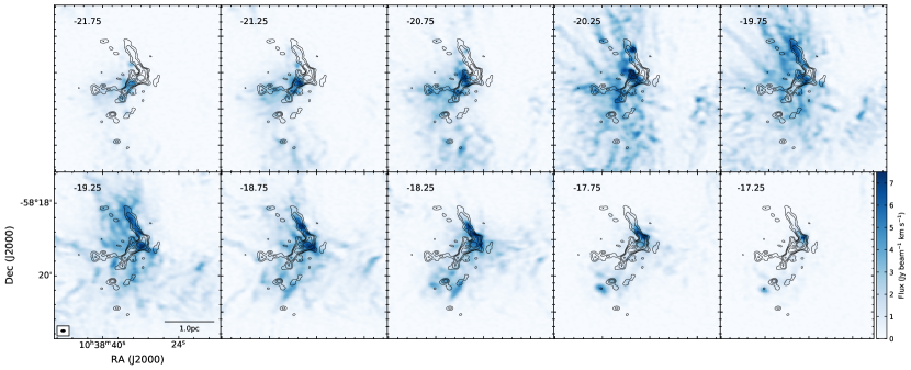
Figure 6 illustrates the $\rm C^{18}O$(2-1) emission, integrated over every 0.5 km s^-1 from -22.0 to -17.0 km s^-1. As in Figure 5, filamentary structures are seen near the systemic velocity of -20 km s^-1. At least three of the $\rm C^{18}O$(2-1) filaments have corresponding detections in the continuum at a 2$\sigma$ level and hence are most likely real features, rather than sidelobe artifacts. The most prominent filament is associated with the NE-SW continuum filament and is clearly seen from -20.0 km s^-1 to -17.0 km s^-1. The NW-SE filament appears more complicated in $\rm C^{18}O$(2-1) and is not well described as being a coherent $\rm C^{18}O$ filamentary structure. Therefore we carry out a virial analysis only for the NE-SW filament.

As shown by Fiege & Pudritz (2000), a pressure-confined, non-rotating, self-gravitating, filamentary (i.e., length $\gg$ width) magnetized cloud that is in virial equilibrium satisfies

$$\frac{P_{e}}{P_{f}}=1-\frac{m_{f}}{m_{\rm vir,f}}\left(1-\frac{M_{f}}{|W_{f}|}\right)$$ (1)

where $P_{f}$ is the mean total pressure in the filament, $P_{e}$ is the external pressure at its surface, $m_{f}$ is its mass per unit length, $m_{\rm vir,f}=2\sigma_{f}^{2}/G$ is its virial mass per unit length, and $M_{f}$ and $W_{f}$ are the gravitational energy and magnetic energy per unit length, respectively. Here, because of the observational difficulties of measuring the surface pressure and magnetic fields, we ignore the surface term and magnetic energy term, i.e., only considering the balance between gravity and internal pressure support.

Figure 6: 7-m $\rm C^{18}O$(2-1) emission integrated over 0.5 km s^-1 intervals, as indicated in the upper left of each panel, from -22.0 to -17.0 km s^-1. The black contours show the 7m array 1.3 mm continuum emission. The contour levels are 1.7 mJy beam^-1$\times$ (4, 10, 20, 50, 100).

Figure 7: (a) Column density map made with Herchel sub-mm continuum data, overlaid on the 7-m array continuum emission in contours. The contour levels are 1.7mJy beam^-1$\times$ (4, 10, 20, 50, 100). The ALMA synthesized beam is shown in the lower left corner, while the resolution of the Herschel-derived mass surface density map is shown in the lower right. The red rectangles dilineate the position of the NE-SW filament and its division into four strips, numbered 1 to 4 from south to north. (b) $\rm C^{18}O$(2-1) spectra of the four strips of the NE-SW filament and the total (see legend). The green lines show primary gaussian component fits to these spectra.

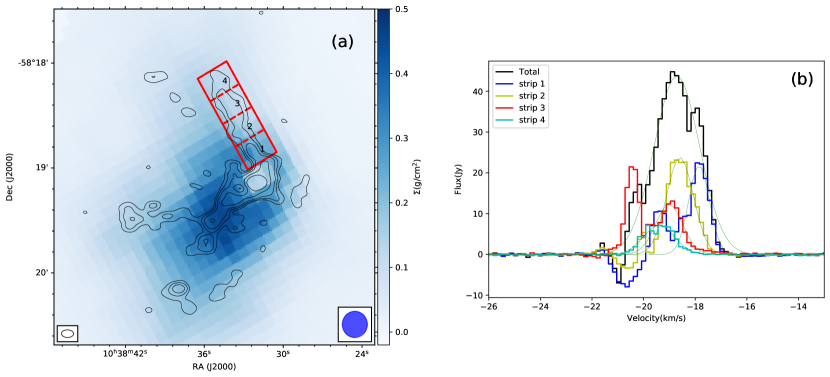
To measure the properties of the filament we show in Figure 7a a 60″$\times$ 20″ rectangle that closely encompasses the NE-SW filament, which we use to define the filament boundary. From the Herschel-SED-derived mass surface density map we find average values of $\Sigma_{\rm sed}$ in the strips ranging from 0.25 $\rm g\>cm^{-2}$ (in Strip 1 that is closest to the center of G286) to 0.12 $\rm g\>cm^{-2}$ (in Strip 4) (see Table 1). The mass in each region is then estimated, with values of between $M_{\rm sed}=$ 26 and 53 $M_{\odot}$. For comparision, we also calculate masses from the 1.3 mm continuum flux, assuming a temperature of 20 K and other dust properties following Cheng et al. (2018). We find the 1.3 mm-derived mass estimates are about a factor of two smaller than that measured from the Herschel-SED fitting method. Since the ALMA 7-m array observations only probe scales up to $\sim$ 19″, they are likely to be missing some flux from the filament leading to an underestimation of the masses, and so here we adopt the Herschel-SED-derived mass estimates for the virial analysis.

The 60″ length of the filament corresponds to 0.73 pc at an assumed distance of 2.5 kpc. We assume a 10% uncertainty in the distance (e.g., Barnes et al., 2010). Without direct observational constraints, we further assume the filament axis is inclined by an angle $i=60^{\circ}$ to the line of sight (90^∘ would be in the plane of the sky). If an inclination angle of 90 or 30^∘ were to be adopted, then the length estimates would differ by factors of 1.15 and 0.577, respectively. Thus the actual the length of the filament is assumed to be 0.84 pc (or 3/4 of this from the centers of Strip 1 to Strip 4). Thus the overall mass per unit length of the filament is $m_{\rm sed,f}\sim 170\>M_{\odot}\>{\rm pc}^{-1}$, with Strip 1 having a higher value of $\sim 250\>M_{\odot}\>{\rm pc}^{-1}$.

The mean line-of-sight velocity and velocity dispersion of the filament are measured from the average $\rm C^{18}O$ spectra inside the rectangular regions. To reduce contamination from surrounding ambient gas at the systemic velocity, we utilize the image cube made with only the 7-m array data (i.e., without feathering with the TP data), as illustrated in Figure 7b. We perform gaussian fitting to measure the average centroid velocity $\overline{v}_{f}$ and velocity dispersion $\sigma_{\rm C^{18}O}$. For strips 1 and 3, two Gaussian components are used for a better fitting. We then compare the $\rm C^{18}O$  spectra with the spectra of denser gas tracers like $\rm DCO^{+}$  and found that only one component is associated with these tracers. This primary component is shown in green lines in Figure 7b and is used for further analysis.

The values of $\overline{v}_{f}$ show a steady progression from $-17.85\>$km s^-1 in Strip 1 to $-19.40\>$km s^-1 in Strip 4, which corresponds to an overall velocity gradient of $2.84\>{\rm km\>s^{-1}\>pc}^{-1}$ using plane-of-sky projected distance or $2.46\>{\rm km\>s^{-1}\>pc}^{-1}$ for the assumed $60^{\circ}$ inclination. We can compare these kinematics to the IRDC filament studied by Hernandez et al. (2011, 2012), which has a length of 3.77 pc on the sky (4.35 pc for the assumed $60^{\circ}$ inclination) and also had its $\rm C^{18}O$(2-1) emission analyzed in 4 strips. Here the velocities did not show a steady progression, but showed differences of about 0.5 km s^-1 from strip to strip, i.e., corresponding to velocity gradients of about $0.53\>{\rm km\>s^{-1}\>pc}^{-1}$ in the plane of the sky. The larger and more systematic velocity gradient shown in the NE-SW filament in G286 may be the result of acceleration due to infall into the protocluster potential. Strip 4 has a mean velocity similar to that of the ambient, larger-scale gas in the region, while Strip 1, closer in projection to the protocluster center, is redshifted with respect to this velocity. Thus in this scenario the Strip 4 end of the filament is closer to us than the protocluster center.

If the velocity change from Strip 4 to Strip 1, i.e., $+1.55\>{\rm km\>s}^{-1}$, is due to infall in the protocluster potential, then we can use this information to constrain the mass of the protocluster. Assuming an uniform distribution of matter in a spherical protocluster clump of radius $L$, the change in potential from the edge to the center is $GM/(2L)$. If material starts at rest at radius $L$, i.e., the Strip 4 position, and then accelerates to velocity $v_{1}$, of which we observe $v_{1}\>{\rm cos}i$, then the mass inside radius $L$ is

$$M=\frac{232}{{\rm cos}^{2}i\>{\rm sin}\>i}\left(\frac{v_{\rm 1,obs}}{\rm km/s}\right)^{2}\left(\frac{L_{\rm obs}}{\rm pc}\right)\>M_{\odot}.$$ (2)

For an observed length $L_{\rm obs}$ from the center of Strip 4 to the center of Strip 1 of 0.55 pc (i.e., 3/4 of 0.73 pc) and a line of sight velocity difference of 1.55 km s^-1 , we thus estimate the dynamical mass to be $1410\>M_{\odot}$, assuming $i=60^{\circ}$. If an inclination angle of 30^∘ or 70^∘ is adopted, the mass would be 814 or $2780\>M_{\odot}$, respectively. This estimation based on filament infall kinematics is broadly consistent with that derived from Herschel-SED fitting, i.e., $\sim 2900\>M_{\odot}$ for the region defined by the larger ellipse aperture in Figure 1. Note, for this SED-based method, we expect $\sim$50% uncertainty in the mass estimation due to dust opacity and distance uncertainties.

Considering the internal dynamics of the filament, in order to account for support against gravity from both thermal and non-thermal motions of the gas, we subtract the thermal component of broadening of the $\rm C^{18}O$(2-1) line from the measured velocity dispersion (in quadrature, assuming a temperature of 20 K) and add back the sound speed to obtain the total 1D velocity dispersion, $\sigma_{f}$, i.e.,

$$\sigma_{f}=\left(\sigma_{\rm nth}^{2}+\sigma_{\rm th}^{2}\right)^{1/2}\\ =\left(\sigma_{\rm C^{18}O}^{2}-\frac{k_{B}T}{\mu_{\rm C^{18}O}m_{p}}+\frac{k_{B}T}{\mu_{p}m_{p}}\right)^{1/2}$$ (3)

where $\mu_{p}$ = 2.33 is the mean molecular weight assuming $n_{\rm He}=0.1n_{\rm H}$ and $\mu_{\rm C^{18}O}$ is the molecular weight of $\rm C^{18}O$. We have then carried out a virial analysis for each of the four strips (see Table 1). Note, for Strips 1 and 3 we fit the spectra with two gaussian components and utilize the component that is more clearly associated with the filament. For example, in Strip 3, the velocity component near -20.5 km s^-1  is contributed by another gas clump to the north-west of the filament.

The values of $m_{f}/m_{\rm vir,f}$ of the four strips range from 0.60 to 2.39. Given the systematic uncertainties in measuring the masses and lengths of the structures that combine to be at least $\sim 50\%$, these values are consistent with the filament being in approximate virial equilibrium, even without accounting for surface pressure and magnetic support terms. We also note that the values of $m_{f}/m_{\rm vir,f}$ grow, i.e., becoming less gravitationally bound, as one progresses from Strip 4 to Strip 1. This may indicate that infall motions and/or tidal forces towards the center of the protocluster act to stabilize the filament.

5 Kinematic properties of the dense core sample

Figure 8: (a) $\rm C^{18}O$ integrated intensity map using combined 7-m + 12-m array data. Red, green and blue contours show emission integrated from -23 to -21 km s^-1, -21 to 19 km s^-1  and -19 to -17 km s^-1, respectively. The contours start from 4$\sigma$ in step of 2$\sigma$, with $\sigma$ = 0.1 Jy beam^-1$\cdot$ km s^-1. The grey scale image is the 1.0″resolution 7-m + 12-m array combined 1.3 mm continuum image. (b) Same as panel (a), but for $\rm N_{2}D^{+}$(3-2). The contours start from 4$\sigma$ in step of 2$\sigma$, with $\sigma$ = 0.025 Jy beam^-1$\cdot$ km s^-1. (c) Same as panel (a), but for $\rm DCO^{+}$(3-2). The contours start from 4$\sigma$ in step of 2$\sigma$, with $\sigma$ = 0.03 Jy beam^-1$\cdot$ km s^-1. (d) Same as panel (a), but for $\rm DCN$(3-2). The contours start from 4$\sigma$ in step of 2$\sigma$, with $\sigma$ = 0.03 Jy beam^-1$\cdot$ km s^-1.

Figure 9: An example of the spectral line fitting for G286c5. Here we use one gaussian component to fit the spectra of $\rm N_{2}D^{+}$(3-2), $\rm DCO^{+}$(3-2) and $\rm DCN$(3-2), and two components for $\rm C^{18}O$(2-1).

Cheng et al. (2018) analysed the mass distribution of dense cores towards the central region of G286 (about 2.2′$\times$1.5′), where the uv coverage of the observation allows imaging with $\sim$1″  resolution. Here we carry out a kinematic follow-up study on the dense core sample in this region.

Figure 8 shows the integrated intensity map of $\rm C^{18}O$(2-1), $\rm N_{2}D^{+}$(3-2), $\rm DCO^{+}$(3-2) and $\rm DCN$(3-2) in the central region, with three velocity ranges shown in different colors. This map is similar to the 12-m + 7-m moment maps in Figure 4, but emphasizes relatively weaker features that might be missing in Figure 4 due to higher noise resulting from its wider velocity range. Most cores in this region have significant detection from at least one of the three dense gas tracers: $\rm N_{2}D^{+}$(3-2), $\rm DCO^{+}$(3-2) and $\rm DCN$(3-2), and this allows us to measure the centroid velocity and velocity dispersion for each dense core.

5.1 Review of the core sample based on dust continuum emission

Cheng et al. (2018) reported different numbers of identified cores, ranging from 60 to 125, depending on the detection algorithm and parameter choices of these algorithms. Here we adopt the fiducial dendrogram identified core sample with a base threshold of 4$\sigma$, a delta threshold of 1$\sigma$, along with a minimum area of half a synthesized beam size. This parameter combination yields 76 cores.

In Table 3 we list the properties of the dense core sample. The cores are here named as G286c1, G286c2, etc., with the numbering order from highest to lowest core mass. The masses are estimated to range from 0.19 $M_{\odot}$ to 80 $M_{\odot}$, assuming a constant temperature of 20 K for each core (see Cheng et al. (2018) for more details). The radius is evaluated as $R_{c}$ = $\sqrt{A/\pi}$, where $A$ is the projected area of the core. The median radius is 0.011 pc, similar to the spatial resolution ($\sim$1″, 2500 AU), indicating many cores are not well resolved. Note that we adopt the core area returned by Dendrogram, which is defined with an isophotal boundary at a certain flux level, i.e., the level where two cores merge together or the 4$\sigma$ flux threshold for isolated cores. So the core area or radius could be underestimated in a crowded field.

We then evaluate the mean mass surface density of the cores as $\Sigma_{c}\equiv M/A$. The median mass surface density of our sample is $\sim$ 0.65 g cm^-2 and all the cores have values $\gtrsim 0.4\>$g cm^-2. We also evaluate the mean H nuclei number density in the cores, $n_{{\rm H},c}\equiv M_{c}/(\mu_{\rm H}V)$, where $\mu_{\rm H}$ = 1.4$m_{\rm H}$ is the mean mass per H assuming $n_{\rm He}$ = 0.1 $n_{\rm H}$ and $V=4\pi R_{c}^{3}/3$. The mean value of log₁₀($n_{{\rm H},c}/{\rm cm}^{-3}$) is 6.88, with a standard deviation of 0.24.

5.2 Spectral fitting

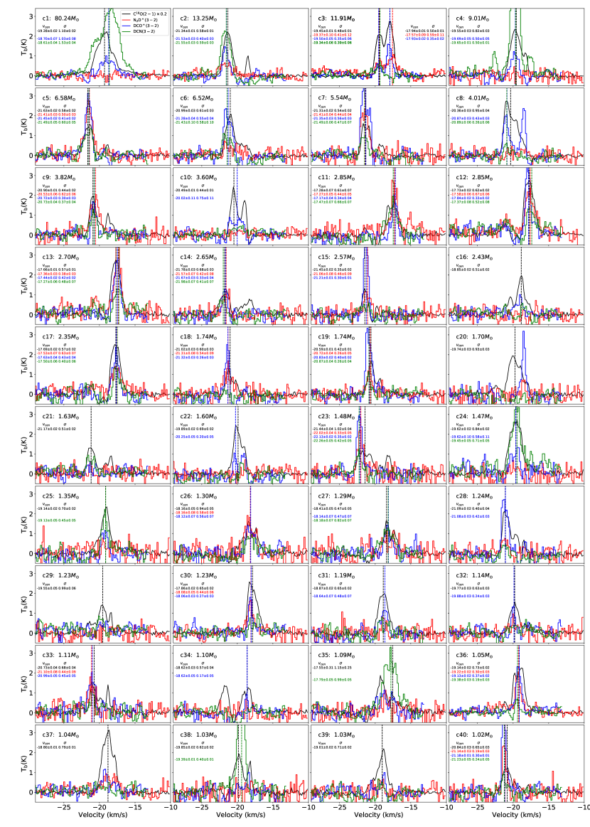
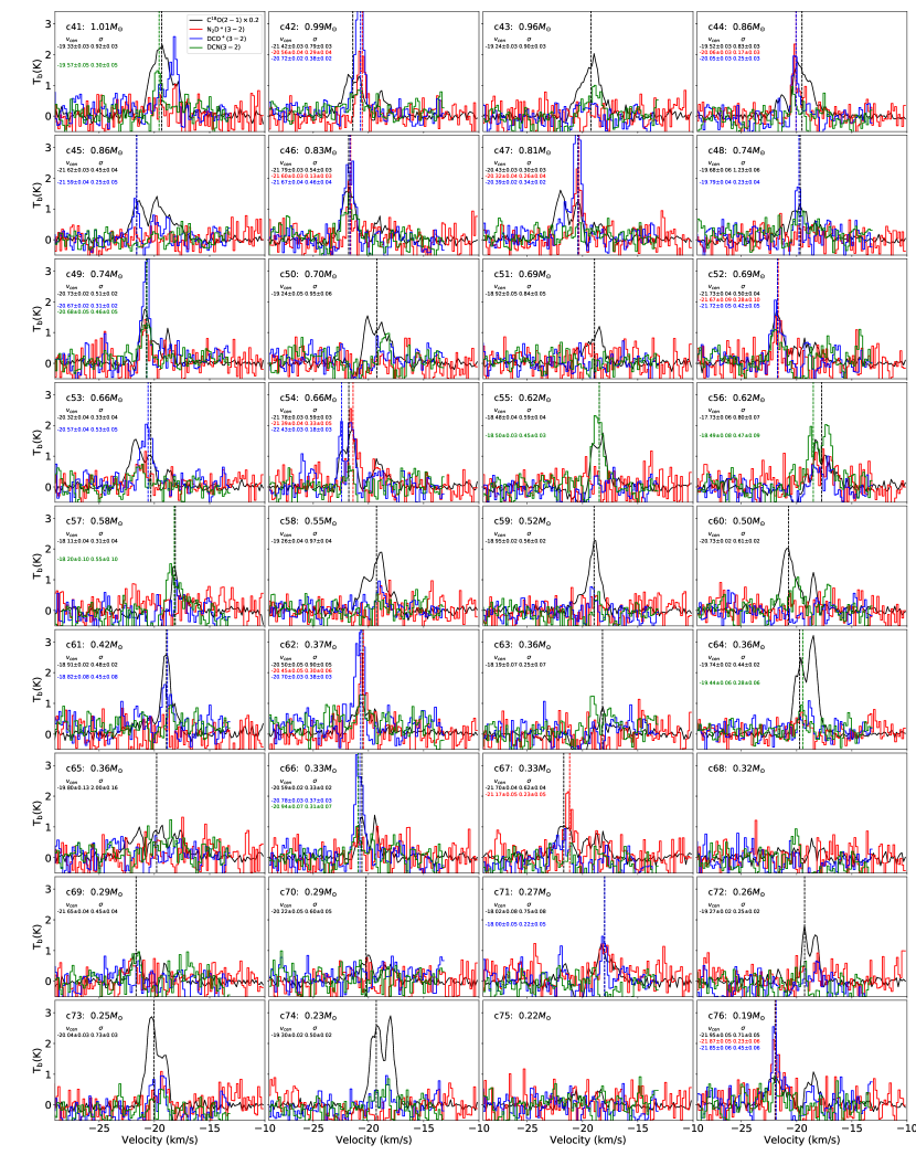
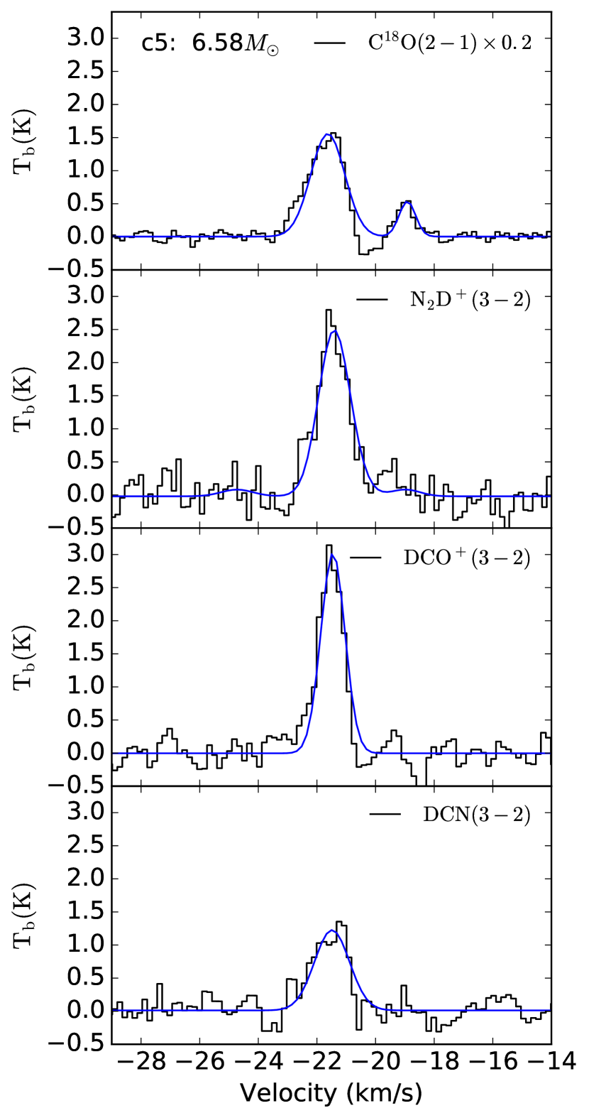
We extract the average $\rm C^{18}O$(2-1), $\rm N_{2}D^{+}$(3-2), $\rm DCO^{+}$(3-2) and $\rm DCN$(3-2) spectra of each core, which are shown in Figure 16 and Figure 17. Among the four tracers $\rm C^{18}O$ is the strongest for almost all the cores, and sometimes the $\rm C^{18}O$ profiles can be complex. Other lines are relatively weak and only detected for part of the core sample.

To measure the centroid velocity and velocity dispersion of each core we only fit spectra with well defined profiles, i.e., those with a peak greater than a certain threshold value. Here we adopt a 4$\sigma$ criterion for this threshold value. Since the noise levels of the average spectra vary for different cores (depending on the pixel numbers in the core, etc.), we estimate the rms noise separately for each core and each line using the signal-free channels. This signal to noise criterion gives 74 cores detected in $\rm C^{18}O$(2-1)(97%), 27 in $\rm N_{2}D^{+}$(3-2)(36%), 45 in $\rm DCO^{+}$(3-2)(59%) and 29 in $\rm DCN$(3-2)(38%). We also checked the single pixel spectra at the continuum peak of each core and found that the vast majority have similar line profiles as the averaged spectra, but the signal to noise ratios are usually lower, so we proceed with our analysis using the core-averaged spectra.

We characterize the $\rm C^{18}O$(2-1) spectra with 1-d gaussian fitting using the curve_fit function in the Scipy.optimize python module. Most cores can be well described with a single gaussian component. In general, we expect that $\rm C^{18}O$(2-1) traces lower density envelope gas surrounding the dense core and thus could be more affected by multiple components along the line of sight. In 31 cores where a spectrum has more complex profiles and hence can not be well approximated by a single gaussian, we allow for a second gaussian component.

For the $\rm DCO^{+}$(3-2) and $\rm DCN$(3-2) lines we also perform the gaussian fitting with curve_fit function. For the $\rm N_{2}D^{+}$(3-2) line, to account for the full blended hyperfine components, we use the hyperfine line fitting routine in pyspeckit (Ginsburg & Mirocha, 2011), with the relative frequencies and optical depths for $\rm N_{2}D^{+}$ taken from Dore et al. (2004) and Pagani et al. (2009). These dense gas tracers are usually well described with one gaussian component. Figure 9 shows a example of the line fitting. In particular, in one case (i.e., G286c3), two separate components were clearly required for a good fit for $\rm N_{2}D^{+}$ and $\rm DCO^{+}$. These two components are mostly likely to belong to two separate entities that are not resolved in their continuum emission.

Figure 10: The centroid core velocity and velocity dispersion of each core measured with $\rm C^{18}O$(2-1), $\rm N_{2}D^{+}$(3-2), $\rm DCO^{+}$(3-2) and $\rm DCN$(3-2).

5.3 Comments on individual cores

G286c1: This is the most massive core in G286, with a mass of 80 $M_{\odot}$ and an equivalent radius of 0.036 pc. G286c1 is associated with strong infrared emission and a wide angle bipolar CO outflow (Cheng et al. in prep.), and hence it is already in a relatively evolved protostellar stage. If we adopt a higher temperature such as 70 K, typical of massive protostellar sources (e.g., Zhang & Tan, 2018), then its mass would be $\sim 20\>M_{\odot}$. G286c1 is not detected in $\rm N_{2}D^{+}$(3-2), but we see broad line profiles from $\rm DCO^{+}$(3-2), $\rm DCN$(3-2) and $\rm C^{18}O$(2-1). In particular, there is very strong $\rm DCN$(3-2) emission from -22 to -15 km s^-1 , which is even broader than $\rm C^{18}O$. Our high resolution ALMA observation in Cycle 5 has revealed further fragmentation and substructures in G286c1 (Cheng et al., in prep.). Here, we still use a one-gaussian component to model the spectral lines of G286c1, and the resulting fitting parameters should be treated more cautiously as reflecting the average properties of the core.

G286c3: This is also a massive core, with $\sim 12\>M_{\odot}$. We have detected $\rm C^{18}O$(2-1), $\rm N_{2}D^{+}$(3-2), $\rm DCO^{+}$(3-2) and $\rm DCN$(3-2) towards G286c3. Interestingly, these spectra of $\rm C^{18}O$, $\rm N_{2}D^{+}$ and $\rm DCO^{+}$ all exhibit a double-peak profile, with one peak centered around -19.5 km s^-1  and another at $\sim$ -18km s^-1, though $\rm DCN$ is only detected in one velocity component. Since we expect the deuteratated species such as $\rm N_{2}D^{+}$ and $\rm DCO^{+}$ to be optically thin, these line profiles are more likely to be contributed by two separate entities inside G286c3 instead of a central dip caused by self-absorption. A detailed inspection from the continuum also reveals that G286c3 is very elongated in the NE-SW direction. Thus it is possible that there are further sub-fragmentations in G286c3 that are not identified by our fiducial dendrogram algorithm: e.g., there could be two cores overlapping along the line of sight. Here we use two-component gaussian fitting to model the spectrum of $\rm C^{18}O$, $\rm N_{2}D^{+}$ and $\rm DCO^{+}$, and treat them as two individual cores (i.e., two data points per line in Figure 10). We split the mass of G286c3 assuming that the mass of each component is proportional to the $\rm C^{18}O$ flux for relavent analysis.

G286c4: This core has an estimated mass of $\sim 9\>M_{\odot}$. There is no $\rm N_{2}D^{+}$ detection, but we see very strong $\rm C^{18}O$, $\rm DCO^{+}$ and $\rm DCN$ emission. $\rm DCN$(3-2) has a very strong peak centered at -19.5 km s^-1 , similar to $\rm C^{18}O$ and $\rm DCO^{+}$. Additionally, there are two secondary peaks at around velocity -16 km s^-1  and -23 km s^-1. These may be a real features resulting from unresolved condensations, or more dynamical activities like outflows, but we are unsure about its origin with the current information. Here for $\rm DCN$ we only fit the central major velocity component that is consistent with other tracers.

G286c8, G286c20 and G286c41: These are special in terms of their $\rm DCO^{+}$(3-2) spectra. All three cores have a $\rm DCO^{+}$ peak around -18 km s^-1. For G286c20 and G286c41, $\rm DCO^{+}$ has a large velocity offset ($\sim$1 km s^-1) compared with other tracers, like $\rm C^{18}O$. For G286c8, this offset is even larger ($\sim$3 km s^-1) and there is another obvious $\rm DCO^{+}$ peak around -21 km s^-1, similar with the peaks of $\rm C^{18}O$ and $\rm DCN$ lines. A possible explanation is that G286c8 has a core velocity around -21 km s^-1, as traced by multiple tracers, while the $\rm DCO^{+}$ feature around -18 km s^-1  is not associated with the dense core. From the continuum map we find that all these three cores are close together and lie on a filamentary feature that is only seen in $\rm DCO^{+}$. This filamentary feature is clear in the $\rm DCO^{+}$ channel map and does not appear to be associated with dense dust continuum. Hence we exclude this $\rm DCO^{+}$ velocity component near -18 km s^-1  for G286c8, G286c20 and G286c41 in our analysis.

5.4 Line parameters of different tracers

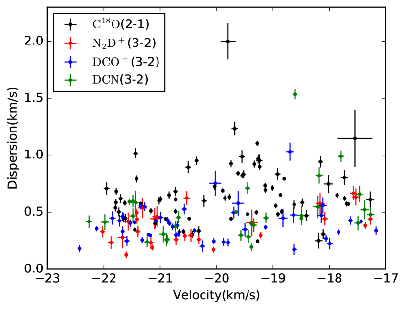
The best-fit parameters of centroid velocity and velocity dispersion are displayed along with the spectral lines in Figure 16 and Figure 17. Figure 10 illustrates the distribution of these parameters, along with their individual uncertainties. As can be seen, the centroid velocities range from -22.5 to -17.0 km s^-1  and there is a modest clustering near -21.5 km s^-1. The velocity dispersions range from 0.1 to 1.0 km s^-1  for deuterated species, while those of $\rm C^{18}O$ are systematically larger. $\rm N_{2}D^{+}$ and $\rm DCO^{+}$ usually give smaller velocity dispersions, with a median value of 0.35 and 0.36 km s^-1, respectively. $\rm DCN$-measured dispersions are larger, with a median value of 0.43 km s^-1. Centroid velocity uncertainties range from 0.01 to 0.08 km s^-1, while velocity dispersion uncertainties vary from 1% to 20%, with a few cases $\gtrsim$30%, depending on the signal to noise ratio and shape of the line profiles.

Figure 11: Left: Line detection status for each core overlaid on the 1.0″  resolution 1.3 mm continuum image in contours. The black crosses denote positions of cores identified via 1.3 mm continuum by Cheng et al. (2018). A red circle indicates a detection of $\rm N_{2}D^{+}$(3-2); a blue circle of $\rm DCO^{+}$(3-2); and a green circle of $\rm DCN$(3-2). Right: Core velocity map overlaid on the 1.0″  resolution 1.3 mm continuum image shown in contours and greyscale. The core velocity is determined by averaging the results from $\rm N_{2}D^{+}$, $\rm DCO^{+}$ and $\rm DCN$(see text). The colored circles indicate the velocity of the 54 dense core that are detected in at least one deuterated tracer. Overall the velocity distribution can be described as being composed of two velocity groups that are spatially distinct, with an approximate boundary shown by the dashed green line.

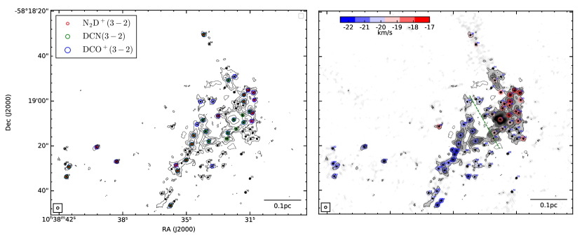
Figure 11 illustrates the line detection situation of the core sample, with different colored circles denoting detections in $\rm N_{2}D^{+}$(3-2), $\rm DCO^{+}$(3-2) and $\rm DCN$(3-2). $\rm C^{18}O$(2-1) is detected for almost all the cores (except c68, c75) and hence is not shown here. As already apparent in Figure 8, $\rm DCN$(3-2) is mostly detected in the central region, while $\rm N_{2}D^{+}$(3-2) and $\rm DCO^{+}$(3-2)-detected cores are more widespread. Overall we have 54 cores that are detected in at least one of these three dense gas tracers. In particular, all the cores with $\rm N_{2}D^{+}$ detection also have strong $\rm DCO^{+}$ emission.

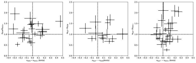
The cores that are detected in more than one line are of particular interest, since differences in fitted parameters could be a reflection of chemical differentiation. There are 14 cores that are detected in all three lines; 26 cores that are detected in both $\rm N_{2}D^{+}$ and $\rm DCO^{+}$; 14 in both $\rm N_{2}D^{+}$ and $\rm DCN$; and 21 in both $\rm DCO^{+}$ and $\rm DCN$. Figure 12 illustrates the differences in fitted parameters of these species when commonly detected. From this figure we see that there is no significant offset in centroid velocity or velocity dispersion as derived from the different species. This similarity in velocity distributions is expected if these species are tracing the same molecular gas material.

For the centroid velocities, the median offsets between $\rm N_{2}D^{+}$ and $\rm DCO^{+}$, $\rm N_{2}D^{+}$ and $\rm DCN$, and $\rm DCO^{+}$ and $\rm DCN$ are 0.07, 0.09, 0.03 km s^-1, respectively. The sampling error of the velocity offset distribution due to the finite number of cores is estimated to be about 0.04 km s^-1, so these offsets are not very significant.

The 1d velocity dispersion $\sigma$ are generally consistent among different tracers within a factor of 2. The median values of $\sigma_{\rm DCN}/\sigma_{\rm DCO^{+}}$, $\sigma_{\rm N_{2}D^{+}}/\sigma_{\rm DCN}$ and $\sigma_{\rm N_{2}D^{+}}/\sigma_{\rm DCO^{+}}$ are 1.16, 0.99 and 0.95, respectively. The observed scatter is consistent with the fitting uncertainties.

We next compare dense core centroid velocities with the larger-scale gas reservoir (or envelope) traced by $\rm C^{18}O$. Previous studies in relatively low-mass environments have shown that cores mostly have subsonic core-to-envelope motions (e.g., Walsh et al., 2004, 2007; Kirk et al., 2007; Walker-Smith et al., 2013). Our work here provides a measure of core-to-envelope motions within a more massive protocluster. Additionally, most previous works measured the centroid velocity offset between $\rm C^{18}O$ and $\rm N_{2}H^{+}$. Here we have observations of lines from deuterated species like $\rm N_{2}D^{+}$, $\rm DCO^{+}$ and $\rm DCN$, which should be better tracers of localized dense cores, rather than more extended filaments, and usually not affected by multiple velocity components that may complicate the interpretation (e.g., Henshaw et al., 2014; Ragan et al., 2015).

Figure 12: Core centroid velocity differences and relative velocity dispersions as measured from $\rm N_{2}D^{+}$(3-2), $\rm DCO^{+}$(3-2) and DCN(3-2).

Figure 13: Left: Distribution of differences between the velocity of dense cores (determined with deuterated tracers) and centroid velocity of $\rm C^{18}O$. Right: Histogram of the distribution. The green line shows a gaussian fit to this distribution.

As mentioned above, we have 54 cores that are detected in at least one of the three deuterated species. For those detected in more than one line we define the core velocity, $v_{c}$, as an average of the detected centroid velocities, weighted by their measurement uncertainties.

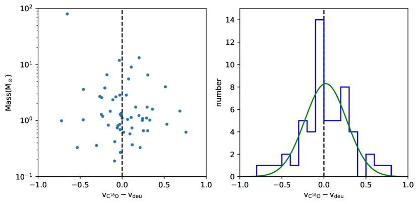
The core velocities $v_{c}$ are illustrated in Figure 11. For cores with only one $\rm C^{18}O$(2-1) component, we compare the difference in centroid velocity between the $\rm C^{18}O$ and $v_{c}$ directly. If multiple CO velocities are found along line of sight, we assume the component closest to $v_{c}$ is the one associated with the core, following the discussion in Kirk et al. (2007). This comparison is shown in Figure 13.

The median value of the velocity offset is 0.01 km s^-1, with a standard deviation of about 0.3 km s^-1. The majority of cores (71%) have core and envelope velocity offsets less than the sound speed of the ambient medium (0.27 km s^-1  for 20 K temperature). This percentage is higher than that in NGC 1333, for which Walsh et al. (2007) found half of their cores have differences greater than the sound speed, but similar to that seen in the Perseus cloud (Kirk et al., 2007). As discussed in Walsh et al. (2004), small relative motions between cores and envelopes could be interpreted as an indication of quiescence on small scales and this would appear to argue against a competitive accretion scenario for star formation (Bonnell & Bate, 2006), in which dense cores gain most of their mass by sweeping up material as they move through the cloud.

5.5 Virial state of dense cores

We now examine the dynamical state of the dense cores, i.e., the comparison of their internal kinetic energy ($E_{K}$) and gravitational energy ($E_{G}$). This ratio is captured by the virial parameter (Bertoldi & McKee, 1992), defined as

$$\alpha\equiv 5\sigma_{c}^{2}R_{c}/(GM_{c})=2aE_{K}/|E_{G}|,$$ (4)

where $\sigma_{c}$ is the intrinsic 1D velocity dispersion of the core and $R_{c}$ is the core radius. The dimensionless parameter $a$ accounts for modifications that apply in the case of non-homogeneous and non-spherical density distributions. For a spherical core with a radial density profile that is a power law $\rho\propto r^{-k_{\rho}}$, then for $k_{\rho}=0,1,1.5,2$, $a=1,10/9,5/4,5/3$. We adopt a fiducial value of $k_{\rho}=1.5$ and $a=5/4$, following McKee & Tan (2003). For a self-gravitating, unmagnetized core without rotation, a virial parameter above a critical value $\alpha_{\rm cr}=2a$ indicates that the core is unbound and may expand, while one below $\alpha_{cr}$ suggests that the core is bound and may collapse.

We measure core 1D velocity dispersions, $\sigma_{c}$, from each of the three dense gas tracers, i.e., $\rm N_{2}D^{+}$, $\rm DCO^{+}$ and $\rm DCN$. As shown above, their line widths can vary for the same core, so we calculate the virial parameters separately using each tracer. We derive the intrinsic velocity dispersion from the observed dispersion following equation (3) (replacing $\rm C^{18}O$ with other species). For the core masses, we use the values estimated assuming a temperature of 20 K, as listed in Table 3.

For core radius we attempt two methods. The first is to use the effective radius calculated from the Dendrogram-returned area (see §5.1). For the second method we adopt a deconvolved size defined as $R_{c}$=$\sqrt{(A-A_{\rm beam})/\pi}$, where $A$ and $A_{\rm beam}$ are the core area and synthesised beam size, respectively. Note that in our core identification process, we have allowed for cores with an area smaller than the synthesized beam size. Here for the virial analysis we ignore the cores with areas smaller than 1.5$\times A_{\rm beam}$, for which the deconvolved sizes could have very large uncertainties. This criterion excludes 34 out of 76 cores.

Figure 14: (a) Virial parameter versus core mass, with radius measured from the dendrogram defined area and velocity dispersion measured with different dense gas tracers, as shown in the legend. The critical value of $\alpha_{\rm cr}=2a\rightarrow 2.5$ is shown by the upper dashed line: cores below this line are gravitationally bound. The lower dashed line shows the virial equilibrium case of $\alpha=a\rightarrow 5/4$. (b) As (a), but with core radius estimated after allowing for beam deconvolution. Small cores, i.e., with areas $>1.5A_{\rm beam}$ are excluded. (c) Same as (a) but we take the linear average of the non-thermal line width measured via different tracers to derive an average virial parameter. (d) Same as (c) but using the deconvolved size.

Figure 15: (a) Distribution of $\rm C^{18}O$(2-1) core centroid velocities (black). Overlaid is the TP $\rm C^{18}O$(2-1) spectrum (averaged over 2.5′  radius aperture) for comparison. The results of core velocities measured with deuterated species are shown in magenta histogram. (b) Same as (a) but only for $\rm N_{2}D^{+}$(3-2). (c) Same as (a) but only for $\rm DCO^{+}$(3-2). (d) Same as (a) but only for $\rm DCN$(3-2). The TP $\rm DCN$(3-2) spectrum is averaged over 1′  radius aperture.

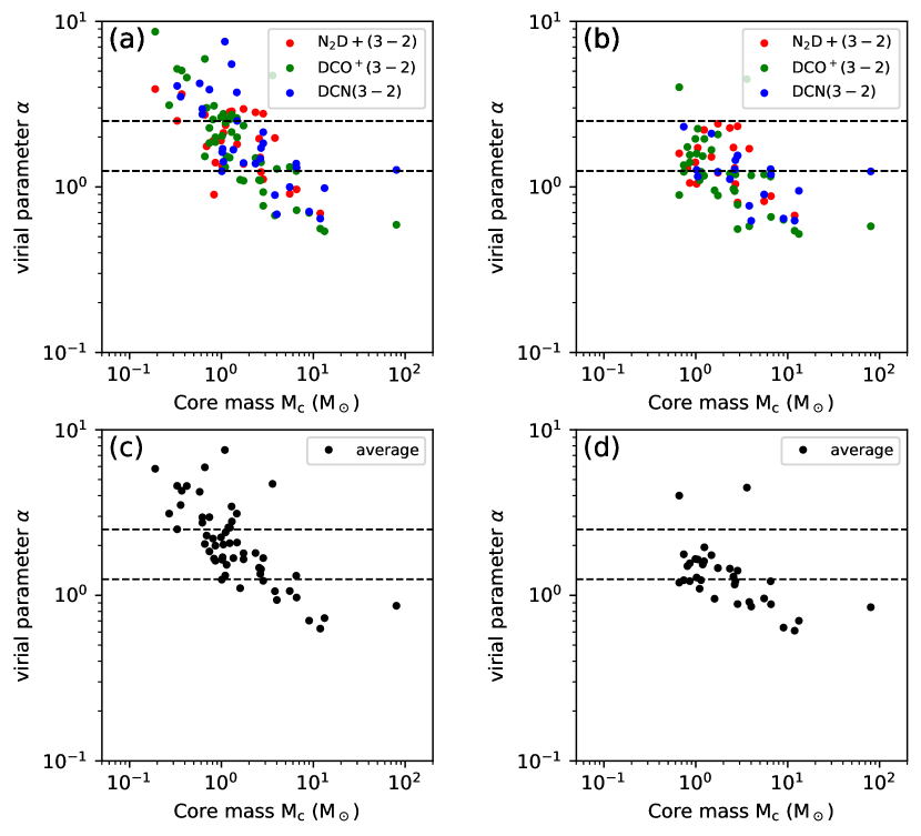
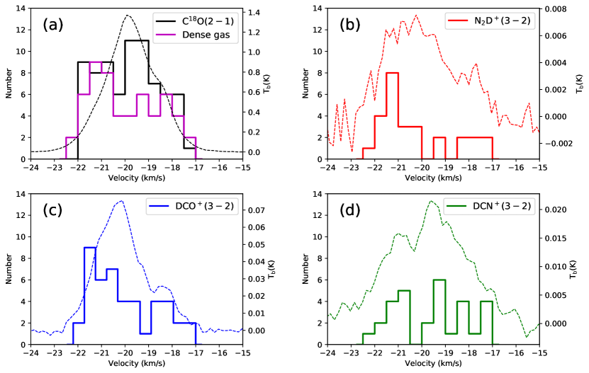
Figure 14a and b display the virial parameters measured with different tracers versus core mass for the two methods described above. In Figure 14c and d we combine the measurements from different tracers by taking the linear average of their non-thermal velocity dispersion in the virial parameter derivation.

We see virial parameters range from 0.5 to 10 as measured by individual dense gas tracers. There is a trend for more massive cores to have smaller virial parameters, but this is generally expected since $\alpha\propto M_{c}^{-1}$. The scatter is significantly reduced for the deconvolved size method, with most measurements ranging from 0.5 to 3. This suggests most data points with virial parameter $>5$ in panel (a) could arise from overestimation in the core radius. We do not find significant systematic differences between different tracers. The median values are 1.35, 1.19, 1.23 for $\rm N_{2}D^{+}$, $\rm DCO^{+}$ and $\rm DCN$, respectively.

The virial parameters estimated by averaging all the available dense gas data for each core show a further reduction in the scatter. For the second method with deconvolved sizes that focus on the larger cores, we obtain a median value of 1.22, and a standard deviation of 0.88. Most cores have a virial parameter that is consistent with a value expected in virial equilibrium, given the uncertainties.

The uncertainties in the derived virial parameters come from uncertainties in measured 1D line dispersion $\sigma_{\rm obs}$, mass and temperature. The fitting error of $\sigma_{\rm obs}$ is typically $\lesssim$20%, resulting in $\sim$ 40% uncertainty in $\sigma_{\rm obs}^{2}$. The assumed temperature will systematically affect estimation of the dense core mass and also the thermal line width component in equation (3). For example, with a typical $\sigma_{\rm DCO^{+}}$ = 0.36 km s^-1, if temperatures of 15 K or 30 K were to be adopted, then the virial parameters would differ by factors of 0.6 and 1.9, respectively. Also considering other uncertainties in the mass estimate, like dust opacity, gas-to-dust mass ratio, dust emission fluxes, and distances, overall, we estimate the absolute virial parameter uncertainties to be about a factor of 2.5. However, this uncertainty factor is itself quite uncertain and includes systematic effects, some of which are not expected to vary that much from core to core.

Given the best case derived average value of $\alpha_{\rm vir}=1.22$, we conclude that the dense cores in G286, which span a wide range of masses from $\lesssim 1\>M_{\odot}$ to $\sim 100\>M_{\odot}$, have properties that are consistent with them being close to virial equilibrium. In this case, self-gravity would have been important in forming the cores and a basic assumption of the turbulent core accretion model of star formation (McKee & Tan, 2003) would be confirmed. However, given the potentially large systematic uncertainties it is difficult to be more certain about whether the dense cores are actually closer to a supervirial or subvirial state, or whether magnetic fields are playing a role in supporting the cores. The situation could be improved in the future with accurate core-scale temperature and magnetic field measurements.

5.6 Core to core velocity dispersion

Table 2: Comparison of core-to-core velocity dispersion and velocity dispersion required for virial equilibrium (in km s^-1)

	$\rm\sigma_{c-c,C^{18}O}$	$\rm\sigma_{c-c,deu}$	$\rm\sigma_{vir}$
blue group	0.83$\pm$0.10	0.78$\pm$0.10	1.48$\pm$0.37
red group	0.75$\pm$0.10	0.79$\pm$0.12	0.96$\pm$0.24
total	1.27$\pm$0.11	1.39$\pm$0.13	1.42$\pm$0.36

The relative motion between dense cores can be quantified using the core-to-core velocity dispersion $\sigma_{\rm c-c}$, i.e., the standard deviation of the core centroid velocities. It can be compared with the velocity dispersion of the large scale diffuse gas out of which these dense cores presumably formed or the initial velocity dispersion of newborn stars, and as such, provides important constraints on theoretical models and simulations of star cluster formation (e.g., Kirk et al., 2010; Foster et al., 2015).

Here our target G286 offers an interesting case of a massive protocluster that is still in the gas-dominated phase and actively forming stars. To measure the core velocity despersion, we show the core velocity distributions measured with $\rm C^{18}O$(2-1), $\rm N_{2}D^{+}$(3-2), $\rm DCO^{+}$(3-2) and $\rm DCN$(3-2) in Figure 15. For comparision the large scale total power spectra of each line are also overlaid. The results combining velocities measured with deuterated tracers (54 cores, see subsection 5.4) are also displayed in Figure 15(a). We then calculate the standard deviation of these distributions, obtaining 1.27 $\pm$ 0.11 km s^-1  for the $\rm C^{18}O$-detected sample, 1.52 $\pm$ 0.21 km s^-1  for the $\rm N_{2}D^{+}$ sample, 1.40 $\pm$ 0.15 km s^-1  for the $\rm DCO^{+}$ cores, 1.50 $\pm$ 0.20 km s^-1  for $\rm DCN$ cores and 1.39 $\pm$ 0.13 km s^-1  for the combined results. The uncertainties here only account for sampling errors due to limited sample size, assuming the data points are drawn from a normal distribution.

In contrast to previous results in nearby cluster-forming clouds like Ophiuchus and Perseus (André et al., 2007; Kirk et al., 2007, 2010), our core velocities cover a wide range from -22.5 to -17 km s^-1  and the distribution is not well approximated with a single gaussian component. This is particularly clear for $\rm N_{2}D^{+}$ and $\rm DCO^{+}$: for these two tracers the core velocities exhibit a bimodal distribution with two velocity groups, which agrees well with the averaged TP spectra. $\rm DCN$ picks up core velocites in a relatively uniform pattern, filling in the gap around -19 km s^-1 , and hence the distribution combining all the deuterated species is more flat, though more cores still cluster in the “blue” group at $\sim$ -21 km s^-1. On the other hand, though the $\rm C^{18}O$ profile can be characterized with a gaussian (with some skewness) peaking aroud -20 km s^-1  and we do have more $\rm C^{18}O$-detected cores close to the systemic velocity (-20 km s^-1  to -19 km s^-1), the $\rm C^{18}O$-measured core velocity distribution is still relatively flat. This indicates that the core to core velocity dispersion we measured here is largely contributed by the global velocity patterns.

The core velocity dispersion $\sigma_{\rm c-c}$ can be compared with the dispersion required for virial equilibrium on the protocluster clump scale $\sigma_{\rm cl,vir}$, and its actual gas velocity dispersion, $\sigma_{\rm cl}$. For $\sigma_{\rm cl,vir}$ we again follow Bertoldi & McKee (1992):

$$\sigma_{\rm cl,vir}=\sqrt{\frac{aGM_{\rm cl}}{5R_{\rm cl}}}.$$ (5)

As with cores, we again adopt $k_{\rho}=1.5$, so that $a=5/4$. We choose a size of $R_{\rm cl}=1.54$ pc, which is the geometric mean of the major and minor axes of the large ellipse boundary shown in Figure 1. From the Herschel-SED-derived mass surface density map we obtain a mass for this region of $\sim 2900\>M_{\odot}$. Thus, $\sigma_{\rm cl,vir}=1.42\pm 0.36$ km s^-1, where the error comes assuming a 50% uncertainty in the mass estimate. We also tried a smaller aperture (by using major and minor axes that are a factor of 1/$\sqrt{2}$ smaller than the current ones) to more closely encompass the region containing dense cores, which gives $\sigma_{\rm cl,vir}=1.54\pm 0.39$ km s^-1. The mass here only accounts for the gas component, since we do not expect significant contribution from stellar mass: Andersen et al. (2017) estimated a total current stellar mass of $\sim 240M_{\odot}$ in a similarly sized region. Thus the observed values of $\sigma_{\rm c-c}$ are comparable or slightly smaller than $\sigma_{\rm cl,vir}$, depending on which tracer is used.

For $\sigma_{\rm cl}$, we measure the line width of average TP spectra of $\rm C^{18}O$(2-1) in this region. The purpose here is to compare core-to-core motions with the spread of motions seen over the region as a whole to reveal how connected the dense cores are to the larger scale gas in the region. A gaussian fit of the $\rm C^{18}O$(2-1) line gives $\sigma_{\rm cl,C^{18}O}$ = 1.09 $\pm$ 0.01 km s^-1. To account for the thermal component we correct this value following equation (3) assuming a temperature of 20 K and obtain $\sigma_{\rm cl}$ = 1.12 km s^-1.

In summary, the 1D dispersion measured in gas tracers, $\sigma_{\rm cl}$ (1.12 $\pm$ 0.01 km s^-1), is slightly smaller, but still consistent with $\sigma_{\rm cl,vir}$ (1.48 $\pm$ 0.37 km s^-1), indicating that the G286 clump could be in approximate virial equilibrium (assuming it is a single, coherent dynamical system) or modestly sub-virial, but it is hard to be more precise given the uncertainties. We also see a range of $\sigma_{\rm c-c}$ values using different tracers and the value using $\rm C^{18}O$(2-1), which includes most cores in this sample, i.e., $\sigma_{\rm c-c,C^{18}O}$ = 1.27 $\pm$ 0.11 km s^-1, is similar to $\sigma_{\rm cl,vir}$, but slight larger than $\sigma_{\rm cl}$. Here the dense core velocity distribution is more flat, while both the $\rm C^{18}O$ core velocities and the TP $\rm C^{18}O$ spectrum cover a similar velocity range. This means there is a deficiency of dense cores near the systemic velocity ($\sim$ 20 km s^-1), where the bulk of the $\rm C^{18}O$-traced gas is located. This deficiency is clearer in the distributions traced by $\rm N_{2}D^{+}$ and $\rm DCO^{+}$, and hence an even larger $\sigma_{\rm c-c}$ is measured with these two tracers. The two velocity groups seen in $\rm N_{2}D^{+}$ and $\rm DCO^{+}$ (at $\sim$ -21 km s^-1and -18km s^-1) are actually spatially distinct (see Figure 4, Figure 8,Figure 11), with the more redshifted cores mostly located in the NE-SW filament and the more blueshifted cores in the NW-SE filament and the E-W filament. A similar velocity pattern is also seen for $\rm C^{18}O$ in Figure 4, indicating the dense cores are still well coupled with the large-scale motions within the cloud.

To better characterize the core-to-core velocity dispersions of the two velocity groups, we adopt a simple boundary to spatially differentiate them, shown as the dashed green line in Figure 11b. The blueshifted subsample (northwest of the boundary) has a core-to-core velocity disperion $\sigma_{\rm c-c,blue}$ of 0.83$\pm$0.10 km s^-1  for $\rm C^{18}O$-detected cores (or 0.78$\pm$0.10km s^-1  for measurements combining $\rm N_{2}D^{+}$, $\rm DCO^{+}$  and $\rm DCN$). Similarly, we have $\sigma_{\rm c-c,red}$ = 0.75$\pm$0.10 km s^-1  for $\rm C^{18}O$  and 0.79$\pm$0.12 km s^-1  for combined dense gas results. For the dispersion required for virial equilibrium, $\sigma_{\rm cl,vir}$, we estimate the mass and radius using two approximate ellipse boundaries for each velocity group (shown in Figure 1), which yields $\sigma_{\rm cl,vir,red}$ = 0.96$\pm$0.24 km s^-1, and $\sigma_{\rm cl,vir,blue}$ = 1.48$\pm$0.37 km s^-1. These numbers are also summarized in Table 2. Therefore, at least for the “blue” group, the core velocity dispersion $\sigma_{\rm c-c}$ is appears to be smaller than $\sigma_{\rm cl,vir}$, potentially indicating it is kinematically cold and sub-virial, perhaps due to coherent motions within a filament. We also see that the dispersion in core velocities for the whole cloud mainly arises from the global velocity pattern of the red and blue groups.

The origin of this velocity pattern is uncertain. In the filament collapse scenario, as observed in some hub-filament systems, accretion flows are channeling gas to the junctions where star formation is often most active (e.g., Kirk et al., 2013; Peretto et al., 2014; Liu et al., 2016). It is possible that these converging flows are reflected in different LOS velocities depending on the 3D configurations. We will presumably have more massive cores in the hub region (near the systemic velocity), but not necessarily a larger number of cores, as suggested by our observations. Smoothly varying velocities along filaments is expected in this picture. We do see indications of a velocity gradient of dense cores along the filaments, but it is not clear in $\rm C^{18}O$, for which the spectra are often complex. Further higher sensitivity observations of $\rm N_{2}H^{+}$ and $\rm NH_{3}$ will help investigate the gas velocity gradient along filaments.

Alternatively, the two main velocity components seen in $\rm N_{2}D^{+}$ and $\rm DCO^{+}$ could be tracing two interacting clouds/filaments, with the central region as the collision interface (e.g., Nakamura et al., 2014). Such a mechanism could be consistent with a larger-scale cloud-cloud collision scenario that has been reported in other star-forming regions (e.g., Furukawa et al., 2009; Fukui et al., 2014; Gong et al., 2017).

Andersen et al. (2017) analysed the stellar population in G286 and found evidence for at least three different sub-clusters associated with the molecular clump based on differences in extinction and disk fractions. It is unclear how the dense gas distribution and ongoing cluster formation might be related with these past star formation events. Future studies of the radial velocity of optically revealed stars, e.g., the velocity dispersion and its distribution will be of great interet to understand the cluster formation in G286.

6 Conclusion

We have studied the gas kinematics and dynamics of the massive protocluster G286.21+0.17 with ALMA using spectral lines of $\rm C^{18}O$(2-1), $\rm N_{2}D^{+}$(3-2), $\rm DCO^{+}$(3-2) and DCN(3-2). The main results are as follows:

1. Morphologically, $\rm C^{18}O$(2-1) traces more extended emission, while $\rm N_{2}D^{+}$(3-2) and $\rm DCO^{+}$(3-2) are more closely associated with the dust continuum. DCN(3-2) is strongly concentrated towards the protocluster center, where no or only weak detection is seen for $\rm N_{2}D^{+}$ and $\rm DCO^{+}$, possibly due to a relatively evolved evolutionary stage in the central region involving chemical evolution at higher temperatures.

2. Based on 1.3 mm continuum, G286 is composed of several pc-scale filamentary structures: the NE-SW filament in northwest, and the NW-SE filament in the southeast, as well as another filament oriented in the E-W direction that is more clearly seen in $\rm DCO^{+}$. The NE-SW filament is associated with redshifted $\rm C^{18}O$ emission while the NW-SE and E-W filament are mainly associated with blueshifted gas. Other tracers show similar velocity structures.

3. We performed a filamentary virial analysis towards the NE-SW filament. We divided the filament into four strips and the values of $m_{f}/m_{\rm vir,f}$ of the four strips range from 0.60 to 2.39. Within the uncertainties, these values are consistent with the filament being in virial equilibrium, without accounting for surface pressure and magnetic support terms. We also detected a steady velocity gradient of 2.84 $\rm km^{-1}pc^{-1}$ along the filament, which may arise from infall motion.

4. We analysed the spectra of 74 continuum dense cores and measureed their centroid velocities and internal velocity dispersions. There are no statistically significant velocity offsets among different tracers. $\rm C^{18}O$ has systematically larger velocity dispersion compared with other tracers.

5. The majority (71%) of the dense cores have subthermal velocity offsets with respect to their surrounding $\rm C^{18}O$ emitting envelope gas, similar as found in previous studies for low-mass star formation environments (e.g., Kirk et al., 2007).

6. We measured the virial parameters of the dense core in G286, which span more than two orders of magnitude in mass. The average value of these virial parameters is close to unity, suggesting the cores are close to virial equilibrium and self-gravity has been important for forming the cores. However, this conclusion is subject to revision if there is a large systematic error in the mass estimates of the cores.

7. The core to core velocity dispersion in G286 is similar to that required for virial equilibrium in the protocluster potential, but with the velocity distribution largely composed of two spatially distinct velocity groups. This indicates that the dense molecular gas has not yet relaxed to virial equilibrium in the protocluster potential, even though the total velocity dispersion would indicate such a condition. The same analysis for the sub-regions corresponding to each velocity group reveals smaller core to core velocity dispersions, with one case consistent with virial equilibrium and the other case indicating a sub-virial state.

Appendix A Properites of dense cores in G286

Table 3: Estimated physical parameters for 1.3 mm continuum cores

core	Ra	Dec	$I_{peak}$	$S_{\nu}$	$M_{c}$	$R_{c}$	$\Sigma_{c}$	$n_{H,c}$
	(∘)	(∘)	mJy beam-1	(mJy)	$M_{\odot}$	(0.01pc)	(g cm-2)	106cm-3
1	159.63383	-58.31897	60.14	420.29	80.24	3.63	4.068	11.71
2	159.63524	-58.32063	15.32	47.19	9.01	1.74	1.994	11.99
3	159.64045	-58.32043	11.20	34.13	6.52	1.92	1.179	6.41
4	159.64373	-58.32201	11.10	34.49	6.58	1.76	1.416	8.39
5	159.63973	-58.32167	11.06	69.42	13.25	2.71	1.209	4.66
6	159.63154	-58.31674	10.03	14.94	2.85	1.05	1.713	16.97
7	159.64328	-58.32094	9.43	29.04	5.54	1.68	1.308	8.12
8	159.63153	-58.31933	9.04	7.07	1.35	0.73	1.694	24.24
9	159.64708	-58.32530	8.73	20.00	3.82	1.43	1.244	9.07
10	159.63546	-58.32133	8.52	5.40	1.03	0.66	1.569	24.74
11	159.63163	-58.31720	8.38	3.23	0.62	0.51	1.574	32.16
12	159.63177	-58.31842	8.30	5.69	1.09	0.68	1.570	24.11
13	159.63045	-58.31534	8.29	14.93	2.85	1.34	1.061	8.28
14	159.63572	-58.31830	7.92	5.31	1.01	0.70	1.380	20.58
15	159.66617	-58.32238	7.90	13.47	2.57	1.56	0.710	4.77
16	159.63329	-58.32012	7.57	7.69	1.47	0.83	1.429	18.01
17	159.62948	-58.31815	7.32	6.79	1.30	0.81	1.325	17.11
18	159.66145	-58.32416	7.31	9.14	1.74	1.26	0.740	6.16
19	159.63511	-58.31409	6.87	62.38	11.91	3.09	0.833	2.82
20	159.63008	-58.31798	6.67	6.77	1.29	0.83	1.258	15.86
21	159.63146	-58.31591	6.52	12.32	2.35	1.23	1.045	8.90
22	159.64112	-58.31903	6.45	21.01	4.01	1.79	0.835	4.87
23	159.62922	-58.31562	6.31	14.14	2.70	1.36	0.975	7.49
24	159.63281	-58.31702	6.16	3.02	0.58	0.58	1.144	20.61
25	159.64503	-58.32397	6.12	13.86	2.65	1.44	0.856	6.23
26	159.63331	-58.31758	6.08	3.27	0.62	0.60	1.160	20.21
27	159.63752	-58.31851	6.06	8.92	1.70	1.13	0.896	8.30
28	159.64744	-58.32461	5.79	5.82	1.11	0.87	0.987	11.89
29	159.64422	-58.32289	5.28	4.33	0.83	0.79	0.875	11.52
30	159.64468	-58.32329	5.22	3.61	0.69	0.73	0.866	12.39
31	159.62961	-58.31916	5.13	6.24	1.19	0.91	0.968	11.16
32	159.63175	-58.32042	5.12	5.04	0.96	0.89	0.814	9.57
33	159.62987	-58.32137	4.50	12.73	2.43	1.45	0.769	5.53
34	159.64877	-58.32960	4.43	7.77	1.48	1.34	0.555	4.34
35	159.63103	-58.32106	4.16	2.89	0.55	0.71	0.724	10.60
36	159.62937	-58.32062	4.12	2.70	0.52	0.68	0.745	11.45
37	159.63976	-58.32276	4.02	8.54	1.63	1.45	0.516	3.71
38	159.63000	-58.32016	4.00	5.38	1.03	0.96	0.737	7.99
39	159.63706	-58.31779	3.92	3.64	0.70	0.87	0.614	7.38
40	159.62838	-58.32134	3.86	2.22	0.42	0.62	0.731	12.26
41	159.63368	-58.31362	3.81	5.43	1.04	1.07	0.610	5.98
42	159.62900	-58.31655	3.77	6.43	1.23	1.16	0.612	5.52
43	159.64888	-58.32789	3.77	5.20	0.99	1.08	0.568	5.49
44	159.64251	-58.31957	3.69	6.50	1.24	1.12	0.660	6.15
45	159.63874	-58.31673	3.64	8.38	1.60	1.44	0.514	3.72
46	159.67328	-58.32603	3.63	5.34	1.02	1.17	0.501	4.49
47	159.63370	-58.31682	3.61	1.91	0.36	0.62	0.643	10.93
48	159.64524	-58.32276	3.46	3.46	0.66	0.90	0.549	6.40
49	159.64849	-58.32509	3.43	3.86	0.74	0.91	0.599	6.90
50	159.63991	-58.32611	3.42	4.53	0.86	1.11	0.472	4.45
51	159.67270	-58.32482	3.38	9.11	1.74	1.56	0.477	3.20
52	159.64614	-58.32435	3.32	1.72	0.33	0.60	0.608	10.60
53	159.64167	-58.31675	3.28	18.88	3.60	2.32	0.449	2.03
54	159.64989	-58.32882	3.27	4.23	0.81	1.00	0.545	5.72
55	159.64225	-58.32300	3.23	1.51	0.29	0.58	0.571	10.29
56	159.63973	-58.32419	3.18	3.90	0.74	0.98	0.517	5.50
57	159.63632	-58.32468	3.12	3.64	0.69	1.01	0.460	4.78
58	159.65086	-58.32812	2.98	3.46	0.66	0.99	0.454	4.82
59	159.63897	-58.32474	2.94	5.99	1.14	1.23	0.502	4.25
60	159.63765	-58.32215	2.90	2.61	0.50	0.88	0.432	5.14
61	159.63372	-58.31557	2.87	1.43	0.27	0.63	0.460	7.63
62	159.63206	-58.32324	2.84	1.69	0.32	0.68	0.467	7.17
63	159.64094	-58.30845	2.83	5.51	1.05	1.25	0.451	3.77
64	159.67355	-58.32445	2.70	1.74	0.33	0.72	0.425	6.13
65	159.64838	-58.31984	2.68	5.75	1.10	1.31	0.425	3.38
66	159.64144	-58.32606	2.67	4.48	0.86	1.17	0.419	3.75
67	159.63598	-58.31504	2.64	1.38	0.26	0.64	0.429	6.98
68	159.67361	-58.32257	2.61	1.94	0.37	0.76	0.431	5.93
69	159.64169	-58.32479	2.60	1.86	0.36	0.74	0.430	6.05
70	159.63645	-58.32321	2.56	6.47	1.23	1.39	0.424	3.18
71	159.63106	-58.32798	2.56	1.49	0.29	0.66	0.434	6.84
72	159.63961	-58.30961	2.55	1.86	0.36	0.75	0.427	5.99
73	159.63557	-58.31262	2.52	1.20	0.23	0.58	0.460	8.35
74	159.63958	-58.31643	2.49	1.31	0.25	0.62	0.436	7.35
75	159.64786	-58.32908	2.47	0.99	0.19	0.53	0.444	8.69
76	159.63002	-58.32627	2.39	1.16	0.22	0.59	0.423	7.46

Appendix B Spectra fitting of the core sample

Figure 16: Spectra of $\rm C^{18}O$(2-1), $\rm N_{2}D^{+}$(3-2), $\rm DCO^{+}$(3-2) and $\rm DCN$(3-2) of 76 continuum cores shown in different colors. The core masses are labeled on the top left. For the spectrum with a peak flux greater than 4 $\sigma$ we perform a gaussian fitting. The returned parameters (centroid velocity, velocity dispersion) for each line are displayed on the top left, in the same color as the corresponding line. The dashed vertical lines indicate the centroid velocity from line fitting (If there are multiple components for $\rm C^{18}O$, only the main component (the one closer to other dense gas tracers, see text) is shown).

Figure 17: Continue of Figure 16.

References

- Adams (2010) Adams, F. C. 2010, ARA&A, 48, 47, doi: 10.1146/annurev-astro-081309-130830
- Andersen et al. (2017) Andersen, M., Barnes, P. J., Tan, J. C., Kainulainen, J., & de Marchi, G. 2017, ApJ, 850, 12, doi: 10.3847/1538-4357/aa9072
- André et al. (2007) André, P., Belloche, A., Motte, F., & Peretto, N. 2007, A&A, 472, 519, doi: 10.1051/0004-6361:20077422
- Barnes et al. (2010) Barnes, P. J., Yonekura, Y., Ryder, S. D., et al. 2010, MNRAS, 402, 73, doi: 10.1111/j.1365-2966.2009.15890.x
- Barnes et al. (2011) Barnes, P. J., Yonekura, Y., Fukui, Y., et al. 2011, ApJS, 196, 12, doi: 10.1088/0067-0049/196/1/12
- Bergin & Tafalla (2007) Bergin, E. A., & Tafalla, M. 2007, ARA&A, 45, 339, doi: 10.1146/annurev.astro.45.071206.100404
- Bertoldi & McKee (1992) Bertoldi, F., & McKee, C. F. 1992, ApJ, 395, 140, doi: 10.1086/171638
- Beuther et al. (2017) Beuther, H., Walsh, A. J., Johnston, K. G., et al. 2017, A&A, 603, A10, doi: 10.1051/0004-6361/201630126
- Bonnell & Bate (2006) Bonnell, I. A., & Bate, M. R. 2006, MNRAS, 370, 488, doi: 10.1111/j.1365-2966.2006.10495.x
- Bressert et al. (2010) Bressert, E., Bastian, N., Gutermuth, R., et al. 2010, MNRAS, 409, L54, doi: 10.1111/j.1745-3933.2010.00946.x
- Busquet et al. (2017) Busquet, G., Fontani, F., Viti, S., et al. 2017, A&A, 604, A20, doi: 10.1051/0004-6361/201730422
- Cheng et al. (2018) Cheng, Y., Tan, J. C., Liu, M., et al. 2018, ApJ, 853, 160, doi: 10.3847/1538-4357/aaa3f1
- Crapsi et al. (2005) Crapsi, A., Caselli, P., Walmsley, C. M., et al. 2005, ApJ, 619, 379, doi: 10.1086/426472
- Dore et al. (2004) Dore, L., Caselli, P., Beninati, S., et al. 2004, A&A, 413, 1177, doi: 10.1051/0004-6361:20034025
- Elmegreen (2007) Elmegreen, B. G. 2007, ApJ, 668, 1064, doi: 10.1086/521327
- Fiege & Pudritz (2000) Fiege, J. D., & Pudritz, R. E. 2000, MNRAS, 311, 85, doi: 10.1046/j.1365-8711.2000.03066.x
- Fontani et al. (2015) Fontani, F., Busquet, G., Palau, A., et al. 2015, A&A, 575, A87, doi: 10.1051/0004-6361/201424753
- Fontani et al. (2018) Fontani, F., Commerçon, B., Giannetti, A., et al. 2018, A&A, 615, A94, doi: 10.1051/0004-6361/201832672
- Foster et al. (2015) Foster, J. B., Cottaar, M., Covey, K. R., et al. 2015, ApJ, 799, 136, doi: 10.1088/0004-637X/799/2/136
- Fukui et al. (2014) Fukui, Y., Ohama, A., Hanaoka, N., et al. 2014, ApJ, 780, 36, doi: 10.1088/0004-637X/780/1/36
- Furukawa et al. (2009) Furukawa, N., Dawson, J. R., Ohama, A., et al. 2009, ApJ, 696, L115, doi: 10.1088/0004-637X/696/2/L115
- Ginsburg & Mirocha (2011) Ginsburg, A., & Mirocha, J. 2011, PySpecKit: Python Spectroscopic Toolkit. http://ascl.net/1109.001
- Ginsburg et al. (2017) Ginsburg, A., Goddi, C., Kruijssen, J. M. D., et al. 2017, ApJ, 842, 92, doi: 10.3847/1538-4357/aa6bfa
- Gong et al. (2017) Gong, Y., Fang, M., Mao, R., et al. 2017, ApJ, 835, L14, doi: 10.3847/2041-8213/835/1/L14
- Gutermuth et al. (2009) Gutermuth, R. A., Megeath, S. T., Myers, P. C., et al. 2009, ApJS, 184, 18, doi: 10.1088/0067-0049/184/1/18
- Hacar et al. (2013) Hacar, A., Tafalla, M., Kauffmann, J., & Kovács, A. 2013, A&A, 554, A55, doi: 10.1051/0004-6361/201220090
- Hartmann et al. (2012) Hartmann, L., Ballesteros-Paredes, J., & Heitsch, F. 2012, MNRAS, 420, 1457, doi: 10.1111/j.1365-2966.2011.20131.x
- Hartmann & Burkert (2007) Hartmann, L., & Burkert, A. 2007, ApJ, 654, 988, doi: 10.1086/509321
- Hennemann et al. (2012) Hennemann, M., Motte, F., Schneider, N., et al. 2012, A&A, 543, L3, doi: 10.1051/0004-6361/201219429
- Henshaw et al. (2014) Henshaw, J. D., Caselli, P., Fontani, F., Jiménez-Serra, I., & Tan, J. C. 2014, MNRAS, 440, 2860, doi: 10.1093/mnras/stu446
- Henshaw et al. (2013) Henshaw, J. D., Caselli, P., Fontani, F., et al. 2013, MNRAS, 428, 3425, doi: 10.1093/mnras/sts282
- Hernandez et al. (2011) Hernandez, A. K., Tan, J. C., Caselli, P., et al. 2011, ApJ, 738, 11, doi: 10.1088/0004-637X/738/1/11
- Hernandez et al. (2012) Hernandez, A. K., Tan, J. C., Kainulainen, J., et al. 2012, ApJ, 756, L13, doi: 10.1088/2041-8205/756/1/L13
- Kirk et al. (2007) Kirk, H., Johnstone, D., & Tafalla, M. 2007, ApJ, 668, 1042, doi: 10.1086/521395
- Kirk et al. (2013) Kirk, H., Myers, P. C., Bourke, T. L., et al. 2013, ApJ, 766, 115, doi: 10.1088/0004-637X/766/2/115
- Kirk et al. (2010) Kirk, H., Pineda, J. E., Johnstone, D., & Goodman, A. 2010, ApJ, 723, 457, doi: 10.1088/0004-637X/723/1/457
- Kong et al. (2015) Kong, S., Caselli, P., Tan, J. C., Wakelam, V., & Sipilä, O. 2015, ApJ, 804, 98, doi: 10.1088/0004-637X/804/2/98
- Krause et al. (2013) Krause, M., Charbonnel, C., Decressin, T., Meynet, G., & Prantzos, N. 2013, A&A, 552, A121, doi: 10.1051/0004-6361/201220694
- Krumholz & McKee (2005) Krumholz, M. R., & McKee, C. F. 2005, ApJ, 630, 250, doi: 10.1086/431734
- Lada & Lada (2003) Lada, C. J., & Lada, E. A. 2003, ARA&A, 41, 57, doi: 10.1146/annurev.astro.41.011802.094844
- Lim et al. (2016) Lim, W., Tan, J. C., Kainulainen, J., Ma, B., & Butler, M. J. 2016, ApJ, 829, L19, doi: 10.3847/2041-8205/829/1/L19
- Liu et al. (2016) Liu, T., Zhang, Q., Kim, K.-T., et al. 2016, ApJ, 824, 31, doi: 10.3847/0004-637X/824/1/31
- Lu et al. (2018) Lu, X., Zhang, Q., Liu, H. B., et al. 2018, ApJ, 855, 9, doi: 10.3847/1538-4357/aaad11
- McKee & Tan (2003) McKee, C. F., & Tan, J. C. 2003, ApJ, 585, 850, doi: 10.1086/346149
- Millar et al. (1989) Millar, T. J., Bennett, A., & Herbst, E. 1989, ApJ, 340, 906, doi: 10.1086/167444
- Molinari et al. (2010) Molinari, S., Swinyard, B., Bally, J., et al. 2010, A&A, 518, L100, doi: 10.1051/0004-6361/201014659
- Molinari et al. (2016) Molinari, S., Schisano, E., Elia, D., et al. 2016, A&A, 591, A149, doi: 10.1051/0004-6361/201526380
- Nakamura & Li (2007) Nakamura, F., & Li, Z.-Y. 2007, ApJ, 662, 395, doi: 10.1086/517515
- Nakamura et al. (2014) Nakamura, F., Sugitani, K., Tanaka, T., et al. 2014, ApJ, 791, L23, doi: 10.1088/2041-8205/791/2/L23
- Ohashi et al. (2016) Ohashi, S., Sanhueza, P., Chen, H.-R. V., et al. 2016, ApJ, 833, 209, doi: 10.3847/1538-4357/833/2/209
- Padoan & Nordlund (2011) Padoan, P., & Nordlund, Å. 2011, ApJ, 730, 40, doi: 10.1088/0004-637X/730/1/40
- Pagani et al. (2009) Pagani, L., Daniel, F., & Dubernet, M. L. 2009, A&A, 494, 719, doi: 10.1051/0004-6361:200810570
- Peretto et al. (2014) Peretto, N., Fuller, G. A., André, P., et al. 2014, A&A, 561, A83, doi: 10.1051/0004-6361/201322172
- Qian et al. (2012) Qian, L., Li, D., & Goldsmith, P. F. 2012, ApJ, 760, 147, doi: 10.1088/0004-637X/760/2/147
- Ragan et al. (2015) Ragan, S. E., Henning, T., Beuther, H., Linz, H., & Zahorecz, S. 2015, A&A, 573, A119, doi: 10.1051/0004-6361/201424948
- Sokolov et al. (2018) Sokolov, V., Wang, K., Pineda, J. E., et al. 2018, A&A, 611, L3, doi: 10.1051/0004-6361/201832746
- Tan (2015) Tan, J. C. 2015, in EAS Publications Series, Vol. 75-76, EAS Publications Series, 105–114
- Tan et al. (2013) Tan, J. C., Kong, S., Butler, M. J., Caselli, P., & Fontani, F. 2013, ApJ, 779, 96, doi: 10.1088/0004-637X/779/2/96
- Tan et al. (2006) Tan, J. C., Krumholz, M. R., & McKee, C. F. 2006, ApJ, 641, L121, doi: 10.1086/504150
- Turner (2001) Turner, B. E. 2001, ApJS, 136, 579, doi: 10.1086/322536
- Walker-Smith et al. (2013) Walker-Smith, S. L., Richer, J. S., Buckle, J. V., et al. 2013, MNRAS, 429, 3252, doi: 10.1093/mnras/sts582
- Walsh et al. (2004) Walsh, A. J., Myers, P. C., & Burton, M. G. 2004, ApJ, 614, 194, doi: 10.1086/423425
- Walsh et al. (2007) Walsh, A. J., Myers, P. C., Di Francesco, J., et al. 2007, ApJ, 655, 958, doi: 10.1086/510193
- Yuan et al. (2018) Yuan, J., Li, J.-Z., Wu, Y., et al. 2018, ApJ, 852, 12, doi: 10.3847/1538-4357/aa9d40
- Zhang & Tan (2018) Zhang, Y., & Tan, J. C. 2018, ApJ, 853, 18, doi: 10.3847/1538-4357/aaa24a
- Zhou et al. (1993) Zhou, S., Evans, Neal J., I., Koempe, C., & Walmsley, C. M. 1993, ApJ, 404, 232, doi: 10.1086/172271