Momentum with Variance Reduction for Nonconvex Composition Optimization

Abstract

Composition optimization is widely-applied in nonconvex machine learning. Various advanced stochastic algorithms that adopt momentum and variance reduction techniques have been developed for composition optimization. However, these algorithms do not fully exploit both techniques to accelerate the convergence and are lack of convergence guarantee in nonconvex optimization. This paper complements the existing literature by developing various momentum schemes with SPIDER-based variance reduction for nonconvex composition optimization. In particular, our momentum design requires less number of proximal mapping evaluations per-iteration than that required by the existing Katyusha momentum. Furthermore, our algorithm achieves near-optimal sample complexity results in both nonconvex finite-sum and online composition optimization and achieves a linear convergence rate under the gradient dominant condition. Numerical experiments demonstrate that our algorithm converges significantly faster than existing algorithms in nonconvex composition optimization.

1 Introduction

A variety of machine learning problems naturally have composition structure and can be formulated as

$$\min_{x\in\mathbb{R}^{d}}\Phi(x)=F(x)+r(x),~{}\text{where }F(x)=f\big{(}g(x)\big{)}.$$

In the above problem, $f:\mathbb{R}^{p}\to\mathbb{R}$ is a differentiable loss function, $g:\mathbb{R}^{d}\to\mathbb{R}^{p}$ is a differentiable mapping and $r:\mathbb{R}^{d}\to\mathbb{R}$ corresponds to a possibly non-smooth regularizer. Such a composition optimization problem covers many important applications including value function approximation in reinforcement learning, risk-averse portfolio optimization (Zhang & Xiao, 2019c), stochastic neighborhood embedding (Liu et al., 2017) and sparse additive model (Wang et al., 2017), etc. We further elaborate the composition structure of these problems in Appendix A.

A simple algorithm to solve the composition problem (P) is the gradient descent algorithm, which, however, induces much computation overhead in the gradient evaluation when the datasize is large. Specifically, consider the following finite-sum formulation of the composition problem (P):

$$\text{\big{(}$\Sigma^{2}$ \!\big{)}}:~{}f(y)=\frac{1}{N}\sum_{k=1}^{N}f_{k}(y),~{}g(x)=\frac{1}{n}\sum_{i=1}^{n}g_{i}(x),$$

where we call the above formulation $(\Sigma^{2})$ as it involves the finite-sum structure in both $f$ and $g$. Due to the composition structure, the gradient of any sample loss $f_{i}(g(x))$ involves the entire Jacobian matrix $g^{\prime}(x)$, which is computational burdensome when $n$ is large. Such a challenge for computing composition gradients has motivated the design of various stochastic algorithms to reduce the sample complexity in composition optimization. In particular, (Wang et al., 2017) proposed a stochastic composition gradient descent (SCGD) algorithm for solving unregulrarized nonconvex composition problems $(\Sigma^{2})$. As the SCGD algorithm suffers from a high stochastic gradient variance and slow convergence rate, more recent works have developed various variance reduction techniques for accelerating stochastic composition optimization. Specifically, the well-known SVRG scheme in (Johnson & Zhang, 2013) has been exploited by (Lian et al., 2016) and (Huo et al., 2018) to develop variance-reduced algorithms for solving the problem $(\Sigma^{2})$ under strong convexity and non-convexity. Other variance reduction schemes such as SAGA (Defazio et al., 2014) and SPIDER (Fang et al., 2018) (a.k.a. SARAH (Nguyen et al., 2017a)) have also been exploited by (Zhang & Xiao, 2019a, c) to reduce the variance in stochastic composition optimization. In particular, the SPIDER-based stochastic composition optimization algorithm proposed in (Zhang & Xiao, 2019c) achieves a near-optimal sample complexity in nonconvex optimization.

Another important and widely-applied technique for accelerating stochastic optimization is momentum, which has also been studied in stochastic composition optimization. For example, (Wang et al., 2017) proposed a momentum-accelerated SCGD algorithm that achieves an improved sample complexity in nonconvex composition optimization, and (Wang et al., 2016) further generalized it to solve regularized $(\Sigma^{2})$ problems that are nonconvex. Recently, (Xu & Xu, 2019) applied the Katyusha momentum developed in (Allen-Zhu, 2017a) to accelerate the SVRG-based composition optimization algorithm and achieved improved sample complexities in convex optimization. While these works exploit momentum to accelerate the practical convergence of composition optimization, their momentum schemes do not provide provable convergence guarantees for nonconvex composition optimization under variance reduction, which is widely-applied in large-scale stochastic optimization. Therefore, the goal of this paper is to develop a momentum with variance reduction scheme for stochastic nonconvex composition optimization. In particular, the algorithm design is desired to resolve the following issues.

• The existing Katyusha momentum with SVRG-based variance reduction proposed in (Xu & Xu, 2019) only applies to convex composition optimization problems and requires two proximal mapping evaluations per-iteration, which induces much computation overhead when the proximal mapping is complex. Can we design a momentum scheme with variance reduction for nonconvex composition optimization that requires less proximal mapping evaluations?

• The existing variance-reduced composition optimization algorithms (without momentum) can achieve a near-optimal sample complexity in nonconvex scenarios. Can we develop a momentum scheme with variance reduction for composition optimization that achieves a near-optimal sample complexity in nonconvex optimization and provides significant acceleration in practice?

• Momentum has not been developed with variance reduction for online nonconvex composition optimization problems. Can we develop a momentum scheme with variance reduction that is applicable to online nonconvex composition optimization problems with provable convergence guarantee?

In this paper, we provide positive answers to the questions mentioned above. Our developed momentum & variance reduction scheme for composition optimization is applicable to both finite-sum and online cases and achieves the state-of-the-art sample complexity results in nonconvex scenarios. We summarize our contributions as follows and compare the sample complexities of all related algorithms in Table 1.

1.1 Our Contributions

We first study a special case of the composition optimization problem $(\Sigma^{2})$ where $N=1$ and only the mapping $g$ has finite-sum structure. To solve such a nonconvex composition problem (referred to as $(\Sigma^{1})$), we propose a stochastic algorithm MVRC-1 that implements both momentum and SpiderBoost-based variance reduction. Our momentum scheme is simpler and computationally lighter than the existing Katyusha momentum studied in (Xu & Xu, 2019). In specific, our momentum scheme requires only one proximal mapping evaluation per-iteration, whereas the Katyusha momentum requires two proximal mapping evaluations per-iteration. Moreover, the momentum scheme of MVRC can adopt very flexible momentum parameter scheduling as we elaborate below.

Under a diminishing momentum, we show that MVRC-1 achieves a near-optimal sample complexity $\mathcal{O}(n+\sqrt{n}\epsilon^{-2})$ in solving the nonconvex composition problem $(\Sigma^{1})$. We further propose a periodic restart scheme to facilitate the practical convergence of MVRC-1 and establish the same near-optimal sample complexity result. Then, under a constant momentum, we show that MVRC-1 also achieves the same near-optimal sample complexity result. Moreover, we establish a linear convergence rate for MVRC-1 under the gradient dominance condition. With a slight modification of algorithm hyper-parameters, we show that MVRC-1 also applies to the online version of the problem $(\Sigma^{1})$ (referred to as $(\mathbb{E}^{1})$) and achieves the state-of-the-art sample complexity in both nonconvex and gradient dominant scenarios under either diminishing or constant momentum.

We further propose the algorithm MVRC-2 that generalizes our momentum with variance reduction scheme to solve the more challenging composition problem $(\Sigma^{2})$, which has finite-sum structure in both $f$ and $g$. With either diminishing or constant momentum and a normalized learning rate, we show that MVRC-2 achieves a near-optimal sample complexity $\mathcal{O}(N+n+\sqrt{\max\{N,n\}}\epsilon^{-2})$ in nonconvex composition optimization. Furthermore, in the corresponding online case (referred to as $(\mathbb{E}^{2})$), we show that MVRC-2 also achieves the state-of-art sample complexity in nonconvex scenario. Please refer to Table 1 for a comprehensive comparison between the sample complexities of our algorithm and those of existing composition optimization algorithms.

Table 1: Comparison of sample complexities of nonconvex composition optimization algorithms. Note that $(\Sigma^{1})$ corresponds to the problem $(\Sigma^{2})$ with $N=1$. $(\mathbb{E}^{1})$ and $(\mathbb{E}^{2})$ correspond to the online versions of $(\Sigma^{1})$ and $(\Sigma^{2})$, respectively.

Problem	Algorithm	Assumption	Momentum	Sample complexity
	CIVR (Zhang & Xiao, 2019c)	$r$ convex	$\times$	$\mathcal{O}(\epsilon^{-3})$
$(\mathbb{E}^{1})$	Our work	$r$ convex	✓	${\mathcal{O}(\epsilon^{-3})}$
	CIVR (Zhang & Xiao, 2019c)	$F$ $v$-gradient dominant	$\times$	$\mathcal{O}(v\epsilon^{-1}\log\epsilon^{-1})$
	Our work	$F$ $v$-gradient dominant	✓	$\mathcal{O}({v\epsilon^{-1}\log\epsilon^{-1}})$
	SAGA (Zhang & Xiao, 2019a)	$r$ convex	$\times$	$\mathcal{O}(n+n^{2/3}\epsilon^{-2})$
	CIVR (Zhang & Xiao, 2019c)	$r$ convex	$\times$	$\mathcal{O}(n+\sqrt{n}\epsilon^{-2})$
$(\Sigma^{1})$	Our work	$r$ convex	✓	${\mathcal{O}(n+\sqrt{n}\epsilon^{-2})}$
	SAGA (Zhang & Xiao, 2019a)	$F$ $v$-gradient dominant	$\times$	$\mathcal{O}((n+\kappa n^{2/3})\log\epsilon^{-1})$
	CIVR (Zhang & Xiao, 2019c)	$F$ $v$-gradient dominant	$\times$	$\mathcal{O}((n+v\sqrt{n})\log\epsilon^{-1})$
	Our work	$F$ $v$-gradient dominant	✓	$\mathcal{O}((n+v\sqrt{n})\log\epsilon^{-1})$
	Basic SCGD (Wang et al., 2017)	$r\equiv 0$	$\times$	$\mathcal{O}(\epsilon^{-8})$
	Accelerated SCGD (Wang et al., 2017)	$r\equiv 0$	✓	$\mathcal{O}(\epsilon^{-7})$
	ASC-PG (Wang et al., 2016)	$r\equiv 0$	✓	$\mathcal{O}(\epsilon^{-4.5})$
$(\mathbb{E}^{2})$	SARAH-Compositional(Yuan et al., 2019)	$r\equiv 0$	$\times$	$\mathcal{O}(\epsilon^{-3})$
	Nested-Spider (Zhang & Xiao, 2019b)	$r$ convex	$\times$	$\mathcal{O}(\epsilon^{-3})$
	Spider+ADMM(Wang, 2019)	$r$ convex	$\times$	$\mathcal{O}(\epsilon^{-3})$
	Our work	$r$ convex	✓	${\mathcal{O}(\epsilon^{-3})}$
	VRSC-PG (Huo et al., 2018)	$r$ convex	$\times$	$\mathcal{O}(N+n+(N+n)^{2/3}\epsilon^{-2})$
	SAGA (Zhang & Xiao, 2019a)	$r$ convex	$\times$	$\mathcal{O}(N+n+(N+n)^{2/3}\epsilon^{-2})$
$(\Sigma^{2})$	SARAH-Compositional(Yuan et al., 2019)	$r\equiv 0$	$\times$	${\mathcal{O}(N+n+\sqrt{N+n}\epsilon^{-2})}$
	Nested-Spider (Zhang & Xiao, 2019b)	$r$ convex	$\times$	$\mathcal{O}(N+n+\sqrt{\max(N,n)}\epsilon^{-2})$
	Spider+ADMM(Wang, 2019)	$r$ convex	$\times$	${\mathcal{O}(N+n+\sqrt{N+n}\epsilon^{-2})}$
	Our work	$r$ convex	✓	${\mathcal{O}(N+n+\sqrt{\max(N,n)}\epsilon^{-2})}$

1.2 Related works

Momentum & variance reduction: Various variance reduction techniques have been originally developed for accelerating stochastic optimization without the composition structure, e.g., SAG (Roux et al., 2012), SAGA (Defazio et al., 2014; Reddi et al., 2016b), SVRG (Johnson & Zhang, 2013; Allen-Zhu & Hazan, 2016; Reddi et al., 2016a, b; Li & Li, 2018), SCSG (Lei et al., 2017), SNVRG (Zhou et al., 2018), SARAH (Nguyen et al., 2017a, b, 2019; Pham et al., 2019) and SPIDER (Fang et al., 2018; Wang et al., 2019). In particular, the SPIDER scheme achieves a near-optimal sample complexity in nonconvex optimization. Momentum-accelerated versions of these algorithms have also been developed, e.g., momentum-SVRG (Li et al., 2017), Katyusha (Allen-Zhu, 2017a), Natasha (Allen-Zhu, 2017b, 2018) and momentum-SpiderBoost (Wang et al., 2019).

Stochastic composition optimization: (Wang et al., 2017) developed the SCGD algorithm for stochastic composition optimization, and (Wang et al., 2016) further developed its momentum-accelerated version. Variance reduction techniques have been exploited to reduce the sample complexity of composition optimization, including the SVRG-based algorithms (Lian et al., 2016; Huo et al., 2018), SAGA-based algorithm (Zhang & Xiao, 2019a), SPIDER-based algorithms (Zhang & Xiao, 2019c, b; Wang, 2019) and SARAH-based algorithm (Yuan et al., 2019). (Xu & Xu, 2019) further applied the Katyusha momentum to accelerate the SVRG-based composition optimization algorithm in convex optimization.

2 Momentum with SpiderBoost for Solving Nonconvex Problems $(\Sigma^{1})$ and $(\mathbb{E}^{1})$

In this section, we develop momentum schemes with the Spider-Boost (Wang et al., 2019) variance reduction technique for solving the nonconvex composition problems $(\Sigma^{1})$ and $(\mathbb{E}^{1})$, which are rewritten below for reference.

$$(\Sigma^{1}):~{} \min_{x\in\mathbb{R}^{d}}\Phi(x)=f\Big{(}\frac{1}{n}\sum_{i=1}^{n}g_{i}(x)\Big{)}+r(x),$$

$$(\mathbb{E}^{1}):~{} \min_{x\in\mathbb{R}^{d}}\Phi(x)=f\big{(}\mathbb{E}_{\xi}g_{\xi}(x)\big{)}+r(x).$$

2.1 Algorithm Design

We present our algorithm design in Algorithm 1 and refer to it as MVRC-1, which is short for Momentum with Variance Reduction for Composition optimization, and “1” stands for the target problems $(\Sigma^{1}),(\mathbb{E}^{1})$. In Algorithm 1, we denote the proximal mapping of function $r$ as: for any $\lambda>0,x\in\mathbb{R}^{d}$,

$$\mathrm{prox}_{\lambda r}(x):=\operatorname*{arg\,min}_{y\in\mathbb{R}^{d}}\Big{\{}r(y)+\frac{1}{2\lambda}\|y-x\|^{2}\Big{\}}.$$ (1)

To elaborate, Algorithm 1 uses the SpiderBoost scheme proposed in (Wang et al., 2019) to construct variance-reduced estimates $\widetilde{g}_{t}$ and $\widetilde{g}_{t}^{\prime}$ of the mapping $g$ and its Jacobian matrix $g^{\prime}$, respectively, and it further adopts a momentum scheme to facilitate the convergence.

Our momentum scheme is simpler than the Katyusha momentum developed for composition optimization in (Xu & Xu, 2019). In particular, our momentum scheme requires only one proximal mapping evaluation per-iteration to update $x_{t+1}$, whereas the Katyusha momentum requires two proximal mapping evaluations per-iteration to update both $x_{t+1}$ and $y_{t+1}$, respectively. Therefore, our momentum scheme saves much computation time when the proximal mapping of the regularizer induces much computation, e.g., nuclear norm regularization, group norm regularization, etc.

Input: $x_{0}\in\mathbb{R}^{d}$; $T,\tau\in\mathbb{N}$; $\lambda_{t}$, $\beta_{t}>0$ and $\alpha_{t}\in[0,1]$;

Initialize: $y_{0}=x_{0}$.

for $t=0,1,\ldots,T-1$ do

        $z_{t}=\left(1-\alpha_{t+1}\right)y_{t}+\alpha_{t+1}x_{t}$,

       if $t\mod\tau=0$ then

               For $(\Sigma^{1}):$ Sample set $\mathcal{A}_{t}=\{1,...,n\}$

               For $(\mathbb{E}^{1}):$ Sample set $\mathcal{A}_{t}$ from the distribution of $\xi$

               $\widetilde{g}_{t}=\frac{1}{|\mathcal{A}_{t}|}\sum_{\xi\in\mathcal{A}_{t}}g_{\xi}(z_{t}),\widetilde{g}_{t}^{\prime}=\frac{1}{|\mathcal{A}_{t}|}\sum_{\xi\in\mathcal{A}_{t}}g_{\xi}^{\prime}(z_{t})$

       else

               For $(\Sigma^{1}):$ Sample subset $\mathcal{A}_{t}$ from $\{1,...,n\}$

               For $(\mathbb{E}^{1}):$ Sample set $\mathcal{A}_{t}$ from the distribution of $\xi$

               $\widetilde{g}_{t}=\widetilde{g}_{t-1}+\frac{1}{|\mathcal{A}_{t}|}\sum_{\xi\in\mathcal{A}_{t}}\big{(}g_{\xi}(z_{t})-g_{\xi}(z_{t-1})\big{)},$

               $\widetilde{g}_{t}^{\prime}=\widetilde{g}_{t-1}^{\prime}+\frac{1}{|\mathcal{A}_{t}|}\sum_{\xi\in\mathcal{A}_{t}}\big{(}g_{\xi}^{\prime}(z_{t})-g_{\xi}^{\prime}(z_{t-1})\big{)},$

        end if

       Compute ${\widetilde{\nabla}F}(z_{t})=\widetilde{g}_{t}^{\prime\top}\nabla f(\widetilde{g}_{t})$,

        $x_{t+1}=\operatorname{prox}_{\lambda_{t}r}(x_{t}-\lambda_{t}{\widetilde{\nabla}F}(z_{t}))$,

        $y_{t+1}=z_{t}+\frac{\beta_{t}}{\lambda_{t}}(x_{t+1}-x_{t})$

end for

Output: $z_{\zeta}$, where $\zeta\stackrel{{\scriptstyle\text{Uniform}}}{{\sim}}\{0,1,\ldots,T-1\}$.

Algorithm 1 (MVRC-1): Momentum with variance reduction for solving composition problems $(\Sigma^{1}),(\mathbb{E}^{1})$

2.2 Convergence Analysis in Nonconvex Optimization

In this subsection, we study the convergence guarantees for MVRC-1 in nonconvex optimization under various choices of the momentum parameter $\alpha_{t}$

We make the following standard assumptions on the objective function.

Assumption 1.

The objective functions in both the finite-sum problem $(\Sigma^{1})$ and the online problem $(\mathbb{E}^{1})$ satisfy

1. Function $f$ is $l_{f}$-Lipschitz continuous, and its gradient $\nabla f$ is $L_{f}$-Lipschitz continuous;

2. Every mapping $g_{\xi}$ is $l_{g}$-Lipschitz continuous, and its Jacobian matrix $g_{\xi}^{\prime}$ is $L_{g}$-Lipschitz continuous;

3. Function $r$ is convex and $\Phi^{*}:=\inf_{x}\Phi(x)>-\infty$.

In particular, the above assumption implies that the gradient of $F=f\circ g$ is Lipschitz continuous with parameter $L_{F}=\ell_{g}^{2}L_{f}+\ell_{f}L_{g}.$ We also make the following assumption on the stochastic variance for the online case.

Assumption 2.

(For the online problem $(\mathbb{E}^{1})$) The online composition optimization problem $(\mathbb{E}^{1})$ satisfies that: there exists $\sigma_{g},\sigma_{g^{\prime}}>0$ such that for all $x\in\mathbb{R}^{d}$,

$$\mathbb{E}_{\xi}\big{[}\|g_{\xi}(x)-g(x)\|^{2}\big{]}\leq\sigma_{g}^{2},~{}\mathbb{E}_{\xi}\big{[}\|g_{\xi}^{\prime}(x)-g^{\prime}(x)\|^{2}\big{]}\leq\sigma_{g^{\prime}}^{2}.$$

Evaluation metric: To evaluate the convergence in nonconvex optimization, we define the generalized gradient mapping at $x$ with parameter $\lambda>0$ as

$${\mathcal{G}}_{\lambda}(x):=\frac{1}{\lambda}\Big{(}x-\operatorname{prox}_{\lambda r}\big{(}x-\lambda\nabla{F}(x)\big{)}\Big{)}.$$ (2)

In particular, when $r$ is convex, ${\mathcal{G}}_{\lambda}(x)=\mathbf{0}$ if and only if $x$ is a stationary point of the objective function $\Phi=F+r$. Therefore, we say a random point $x$ achieves $\epsilon$-accuracy if it satisfies $\mathbb{E}\|{\mathcal{G}}_{\lambda}(x)\|\leq\epsilon$.

We first study MVRC-1 with the choice of a diminishing momentum coefficient $\alpha_{t}=\frac{2}{t+1}$. We obtain the following complexity results. Throughout the paper, we define $G_{0}=2(l_{g}^{4}L_{f}^{2}+l_{f}^{2}L_{g}^{2})$ and use $\mathcal{O}(\cdot)$ to hide universal constants.

Theorem 1 (Diminishing momentum).

Let Assumptions 1 and 2 hold. Apply MVRC-1 to solve the problems $(\Sigma^{1})$ and $(\mathbb{E}^{1})$ with momentum parameters $\alpha_{t}=\frac{2}{t+1},\beta_{t}\equiv\beta\leq(2\sqrt{16L_{F}^{2}+6G_{0}}+8L_{F})^{-1},\lambda_{t}\in[\beta,(1+\alpha_{t})\beta]$.

• For the problem $(\Sigma^{1})$, choose parameters $\tau=\lfloor{\sqrt{n}}\rfloor$, $|\mathcal{A}_{t}|=n$ whenever $t~{}\text{\rm mod}~{}\tau=0$, and $|\mathcal{A}_{t}|=\lfloor{\sqrt{n}}\rfloor$ otherwise. Then, the output satisfies

  $$\mathbb{E}\|{\mathcal{G}}_{\lambda_{\zeta}}(z_{\zeta})\|^{2}\leq\mathcal{O}\Big{(}\frac{\Phi\left(x_{0}\right)-\Phi^{*}}{T\beta}\Big{)}.$$ (3)

  Moreover, to achieve an $\epsilon$-accurate solution, the required sample complexity (number of evaluations of $g,g^{\prime}$) is $\mathcal{O}(n+\sqrt{n}\epsilon^{-2})$.

• For the problem $(\mathbb{E}^{1})$, choose $\tau=\lfloor\sqrt{2\sigma_{0}^{2}\epsilon^{-2}}\rfloor$, $|\mathcal{A}_{t}|=\lceil 2\sigma_{0}^{2}\epsilon^{-2}\rceil$ whenever $t~{}\text{\rm mod}~{}\tau=0$ and $|\mathcal{A}_{t}|=\lfloor\sqrt{2\sigma_{0}^{2}\epsilon^{-2}}\rfloor$ otherwise. Then, the output satisfies

  $$\mathbb{E}\|{\mathcal{G}}_{\lambda_{\zeta}}(z_{\zeta})\|^{2}\leq\mathcal{O}\Big{(}\epsilon^{2}+\frac{\Phi\left(x_{0}\right)-\Phi^{*}}{T\beta}\Big{)}.$$ (4)

  Moreover, to achieve an $\epsilon$-accurate solution, the required sample complexity is $\mathcal{O}(\epsilon^{-3})$.

Therefore, the MVRC-1 algorithm achieves a sublinear $\mathcal{O}(T^{-1})$ convergence rate in both finite-sum and online cases. In particular, the sample complexities of MVRC-1 match the state-of-art near-optimal sample complexities for nonconvex stochastic optimization.

Momentum with periodic restart: We can further use a restart strategy to boost the practical convergence of MVRC-1 under the diminishing momentum scheme. To be specific, consider implementing MVRC-1 $M$ times and denote $\{x_{t,m},y_{t,m},z_{t,m}\}_{t=0}^{T-1}$ as the generated variable sequences in the $m$-th run. If we adopt the initialization scheme $x_{0,m+1}=x_{T-1,m}$ for $m=1,\ldots,M-1$, then it can be shown that (see Section C.1 for the detailed proof)

For $$(\Sigma^{1}) \mathbb{E}\|{\mathcal{G}}_{\lambda_{\zeta}}(z_{\zeta,\delta})\|^{2}\leq\mathcal{O}\Big{(}\frac{\Phi\left(x_{0,1}\right)-\Phi^{*}}{MT\beta}\Big{)},$$:

For $$(\mathbb{E}^{1}) \mathbb{E}\|{\mathcal{G}}_{\lambda_{\zeta}}(z_{\zeta,\delta})\|^{2}\leq\mathcal{O}\Big{(}\epsilon^{2}+\frac{\Phi\left(x_{0,1}\right)-\Phi^{*}}{MT\beta}\Big{)},$$:

where $\zeta$ is uniformly sampled from $\{0,\ldots,T-1\}$ and $\delta$ is uniformly sampled from $\{1,\ldots,M\}$. In particular, by choosing $M=T=\mathcal{O}(\epsilon^{-1})$, we can achieve an $\epsilon$-accurate solution with the same sample complexities as those specified in 1.

The momentum scheme of MVRC-1 also allows to adopt a more aggressive constant-level momentum coefficient, i.e., $\alpha_{t}\equiv\alpha$ for any $\alpha\in(0,1]$. We obtain the following convergence results.

Theorem 2 (Constant momentum).

Let Assumptions 1 and 2 hold. Apply MVRC-1 to solve the problems $(\Sigma^{1})$ and $(\mathbb{E}^{1})$ with momentum parameters $\alpha_{t}\equiv\alpha\in(0,1],\beta_{t}\equiv\beta\leq(4{\sqrt{{{(1+\alpha^{-1})}^{2}}L_{F}^{2}+3{G_{0}}}+4(1+\alpha^{-1}){L_{F}}})^{-1},\lambda_{t}\in[\beta,(1+\alpha)\beta]$.

• For the problem $(\Sigma^{1})$, choose the same $\tau$ and $|\mathcal{A}_{t}|$ as those in item 1 of 1. Then, the output satisfies

  $$\mathbb{E}\|{\mathcal{G}}_{\lambda_{\zeta}}(z_{\zeta})\|^{2}\leq\mathcal{O}\Big{(}\frac{\alpha^{-1}+1}{T\beta}\big{(}\Phi\left(x_{0}\right)-\Phi^{*}\big{)}\Big{)}.$$ (5)

  Moreover, to achieve an $\epsilon$-accurate solution, the required sample complexity is $\mathcal{O}(n+\sqrt{n}\epsilon^{-2})$.

• For the problem $(\mathbb{E}^{1})$, choose the same $\tau$ and $|\mathcal{A}_{t}|$ as those in item 2 of 1. Then, the output satisfies

  $$\mathbb{E}\|{\mathcal{G}}_{\lambda_{\zeta}}(z_{\zeta})\|^{2}\leq\mathcal{O}\Big{(}\!(\alpha^{-1}+1)\Big{(}\epsilon^{2}\!+\!\frac{\Phi(x_{0})-\Phi^{*}}{T\beta}\Big{)}\!\Big{)}.$$ (6)

  Moreover, to achieve an $\epsilon$-accurate solution, the required sample complexity is $\mathcal{O}(\epsilon^{-3})$.

Hence, under the constant momentum, MVRC-1 maintains the near-optimal sample complexities in solving both the finite-sum problem $(\Sigma^{1})$ and the online problem $(\mathbb{E}^{1})$. We note that under the constant momentum, the proof technique of the previous 1 (under diminishing momentum) does not apply, and the proof of 2 requires novel developments on bounding the variable sequences. To elaborate, we need to develop Lemma 3 in Appendix D to bound the difference sequences $\{\|y_{t}-x_{t}\|,\|z_{t+1}-z_{t}\|\}_{t}$ based on the constant momentum scheme. Moreover, appendix E in Appendix D is developed to bound the accumulated constant momentum parameter involved in the series $\sum_{t=0}^{T-1}\|y_{t}-x_{t}\|^{2}$. These developments are critical for obtaining the convergence guarantees and sample complexities of MVRC-1 under constant momentum.

3 Analysis of MVRC-1 under Nonconvex Gradient-dominant Condition

In this subsection, we study the convergence guarantees of MVRC-1 in solving unregularized nonconvex composition problems that satisfy the following gradient dominant condition. Throughout, we denote $F^{*}:=\inf_{x\in\mathbb{R}^{d}}F(x)$.

Assumption 3 (Gradient dominant).

Consider the unregularized problem (P) with $r(x)\equiv 0$. Function $F$ is called gradient dominant with parameter $v>0$ if $~{}\forall x\in\mathbb{R}^{d},$

$$F(x)-F^{*}\leq\frac{v}{2}\left\|\nabla F(x)\right\|^{2}.$$ (7)

The gradient dominant condition is a relaxation of strong convexity and is satisfied by many nonconvex machine learning models. Next, under the gradient dominant condition, we show that MVRC-1 achieves a linear convergence rate in solving the composition problems $(\Sigma^{1})$ and $(\mathbb{E}^{1})$. We first consider the case of diminishing momentum.

Theorem 3 (Diminishing momentum).

Let Assumptions 1, 2 and 3 hold. Apply MVRC-1 to solve the problems $(\Sigma^{1})$ and $(\mathbb{E}^{1})$ with momentum parameters $\alpha_{t}=\frac{2}{t+1},\beta_{t}\equiv\beta\leq(2\sqrt{16L_{F}^{2}+6G_{0}}+8L_{F})^{-1},\lambda_{t}\in[\beta,(1+\alpha_{t})\beta]$.

• For the problem $(\Sigma^{1})$, choose the same $\tau$ and $|\mathcal{A}_{t}|$ as those in item 1 of 1. Then, the output satisfies

  $$\mathbb{E}F({z_{\zeta}})-{F^{*}}\leq\mathcal{O}\Big{(}\frac{v(F\left({{x_{0}}}\right)-{F^{*}})}{T\beta}\Big{)}.$$ (8)

• For the problem $(\mathbb{E}^{1})$, choose the same $\tau$ and $|\mathcal{A}_{t}|$ as those in item 2 of 1. Then, the output satisfies

  $$\mathbb{E}F({z_{\zeta}})-{F^{*}}\leq\mathcal{O}\Big{(}v{\epsilon^{2}}+\frac{v(F\left({{x_{0}}}\right)-{F^{*}})}{T\beta}\Big{)}.$$ (9)

Moreover, to achieve an $\epsilon$-accurate solution, we restart MVRC-1 $M$ times with $y_{0,m+1}=x_{0,m+1}$ being randomly selected from $\{z_{t,m}\}_{t=0}^{T-1}$ and choose $M=\mathcal{O}(\log\frac{1}{\epsilon}),T=\max\{\mathcal{O}(v),\tau\}$. Then,

• For the problem $(\Sigma^{1})$, the required sample complexity is $\mathcal{O}((n+\sqrt{n}v)\log\frac{1}{\epsilon})$.

• For the problem $(\mathbb{E}^{1})$, the required sample complexity is $\mathcal{O}(v\epsilon^{-2}\log\frac{1}{\epsilon})$.

Therefore, MVRC-1 achieves a linear convergence rate in solving both $(\Sigma^{1})$ and $(\mathbb{E}^{1})$ under the gradient dominant condition, and the corresponding sample complexities match the best-known existing results. Furthermore, our algorithm also allows to adopt a constant momentum scheme under the gradient dominant condition and preserves the convergence guarantee as well as the sample complexity. We obtain the following result.

Theorem 4 (Constant momentum).

Let Assumptions 1, 2 and 3 hold. Apply MVRC-1 to solve the problems $(\Sigma^{1})$ and $(\mathbb{E}^{1})$ with parameters $\alpha_{t}\equiv\alpha\in(0,1],\beta_{t}\equiv\beta\leq(4{\sqrt{{{(1+1/\alpha)}^{2}}L_{F}^{2}+3{G_{0}}}+4(1+1/\alpha){L_{F}}})^{-1},\lambda_{t}\in[\beta,(1+\alpha_{t})\beta]$.

• For the problem $(\Sigma^{1})$, choose the same $\tau$ and $|\mathcal{A}_{t}|$ as those in item 1 of 1. Then, the output satisfies

  $${\mathbb{E}}F({z_{\zeta}})-{F^{*}}\leq\mathcal{O}\Big{(}\frac{v(\alpha^{-1}+1)}{T\beta}\big{(}F\left(x_{0}\right)-F^{*}\big{)}\Big{)}.$$ (10)

• For the problem $(\mathbb{E}^{1})$, choose the same $\tau$ and $|\mathcal{A}_{t}|$ as those in item 2 of 1. Then, the output satisfies

  $$\mathbb{E}F({z_{\zeta}})-{F^{*}}\leq\mathcal{O}\Big{(}\!v(\alpha^{-1}\!+\!1)\Big{(}\epsilon^{2}\!+\!\frac{F\left(x_{0}\right)\!-\!F^{*}}{T\beta}\Big{)}\!\Big{)}.$$

To achieve an $\epsilon$-accurate solution, we restart MVRC-1 $M$ times with $y_{0,m+1}=x_{0,m+1}$ being randomly selected from $\{z_{t,m}\}_{t=0}^{T-1}$ and choose $M=\mathcal{O}(\log\frac{1}{\epsilon}),T=\max\{\mathcal{O}(v),\tau\}$. Then,

• For the problem $(\Sigma^{1})$, the required sample complexity is $\mathcal{O}((n+\sqrt{n}v)\log\frac{1}{\epsilon})$.

• For the problem $(\mathbb{E}^{1})$, the required sample complexity is $\mathcal{O}(v\epsilon^{-2}\log\frac{1}{\epsilon})$.

4 Momentum with SPIDER for Solving Nonconvex Problems $(\Sigma^{2})$ and $(\mathbb{E}^{2})$

In this section, we develop momentum schemes with variance reduction for solving the composition optimization problems $(\Sigma^{2})$ and $(\mathbb{E}^{2})$ that have double finite-sum and double expectation structures, respectively, which are rewritten below for reference.

$$(\Sigma^{2}):~{} \min_{x\in\mathbb{R}^{d}}\Phi(x)=\frac{1}{N}\sum_{k=1}^{N}f_{k}\Big{(}\frac{1}{n}\sum_{i=1}^{n}g_{i}(x)\Big{)}+r(x),$$

$$(\mathbb{E}^{2}):~{} \min_{x\in\mathbb{R}^{d}}\Phi(x)=\mathbb{E}_{\eta}f_{\eta}\big{(}\mathbb{E}_{\xi}g_{\xi}(x)\big{)}+r(x).$$

4.1 Algorithm Design

The details of the algorithm design are presented in Algorithm 2, which is referred to as MVRC-2. We note that the MVRC-2 for solving the composition problems $(\Sigma^{2}),(\mathbb{E}^{2})$ are different from the MVRC-1 for solving the simpler problems $(\Sigma^{1}),(\mathbb{E}^{1})$ in several aspects. To elaborate, first, in order to handle the double finite-sum and double expectation structure of $(\Sigma^{2})$ and $(\mathbb{E}^{2})$, MVRC-2 requires to sample both the mapping $g$ and the function $f$. In particular, the sampling of $g$ is independent from that of $g^{\prime}$, which is different from MVRC-1 where they share the same set of samples. Second, MVRC-2 adopts a SPIDER-like variance reduction scheme that uses an accuracy-dependent stepsize $\theta_{t}$, whereas MVRC-1 uses the SpiderBoost variance reduction scheme that adopts a constant stepsize. As we present later, such a conservative stepsize leads to theoretical convergence guarantees for MVRC-2 in solving the more challenging problems $(\Sigma^{2}),(\mathbb{E}^{2})$ and help achieve a near-optimal sample complexity result.

Input: $x_{0}\in\mathbb{R}^{d}$; $T,\tau\in\mathbb{N}$; $\epsilon,\lambda_{t}$, $\beta_{t}>0$ and $\alpha_{t}\in[0,1]$;

Initialize: $y_{0}=x_{0}$.

for $t=0,1,\ldots,T-1$ do

        $z_{t}=\left(1-\alpha_{t+1}\right)y_{t}+\alpha_{t+1}x_{t}$,

       if $t\mod\tau=0$ then

               For $(\Sigma^{2}):$ Sample sets $\mathcal{A}_{t},\mathcal{A}_{t}^{\prime}=\{1,...,n\}$ and $\mathcal{B}_{t}=\{1,...,N\}$

               For $(\mathbb{E}^{2}):$ Sample sets $\mathcal{A}_{t},\mathcal{A}_{t}^{\prime}$ from the distribution of $\xi$ and sample set $\mathcal{B}_{t}$ from the distribution of $\eta$

               $\widetilde{g}_{t}=\frac{1}{|\mathcal{A}_{t}|}\sum_{\xi\in\mathcal{A}_{t}}g_{\xi}(z_{t}),$ $\widetilde{g}_{t}^{\prime}=\frac{1}{|\mathcal{A}_{t}^{\prime}|}\sum_{\xi\in\mathcal{A}_{t}^{\prime}}g_{\xi}^{\prime}(z_{t}),$

               $\widetilde{f}_{t}^{\prime}=\frac{1}{|\mathcal{B}_{t}|}\sum_{\eta\in\mathcal{B}_{t}}\nabla f_{\eta}(\widetilde{g}_{t}).$

       else

               For $(\Sigma^{2}):$ Sample subsets $\mathcal{A}_{t},\mathcal{A}_{t}^{\prime}$ from $\{1,...,n\}$ and $\mathcal{B}_{t}$ from $\{1,...,N\}$

               For $(\mathbb{E}^{2}):$ Sample sets $\mathcal{A}_{t},\mathcal{A}_{t}^{\prime}$ from the distribution of $\xi$ and sample set $\mathcal{B}_{t}$ from the distribution of $\eta$

               $\widetilde{g}_{t}=\widetilde{g}_{t-1}+\frac{1}{|\mathcal{A}_{t}|}\sum_{\xi\in\mathcal{A}_{t}}\big{(}g_{\xi}(z_{t})-g_{\xi}(z_{t-1})\big{)},$

               $\widetilde{g}_{t}^{\prime}=\widetilde{g}_{t-1}^{\prime}+\frac{1}{|\mathcal{A}_{t}^{\prime}|}\sum_{\xi\in\mathcal{A}_{t}^{\prime}}\big{(}g_{\xi}^{\prime}(z_{t})-g_{\xi}^{\prime}(z_{t-1})\big{)},$

               $\widetilde{f}_{t}^{\prime}=\widetilde{f}_{t-1}^{\prime}+\frac{1}{|\mathcal{B}_{t}|}\sum_{\eta\in\mathcal{B}_{t}}\big{(}\nabla f_{\eta}(\widetilde{g}_{t})-\nabla f_{\eta}(\widetilde{g}_{t-1})\big{)}$

        end if

       Compute ${\widetilde{\nabla}F}(z_{t})=\widetilde{g}_{t}^{\prime\top}\widetilde{f}_{t}^{\prime}$,

        $\widetilde{x}_{t+1}=\operatorname{prox}_{\lambda_{t}r}(x_{t}-\lambda_{t}{\widetilde{\nabla}F}(z_{t}))$,

        $x_{t+1}=(1-\theta_{t})x_{t}+\theta_{t}\widetilde{x}_{t+1},\theta_{t}=\min\big{\{}\frac{\epsilon\lambda_{t}}{\|\widetilde{x}_{t+1}-x_{t}\|},\frac{1}{2}\big{\}}$,

        $y_{t+1}=z_{t}+\frac{\beta_{t}}{\lambda_{t}}(x_{t+1}-x_{t})$

end for

Output: $z_{\zeta}$, where $\zeta\stackrel{{\scriptstyle\text{Uniform}}}{{\sim}}\{0,1,\ldots,T-1\}$.

Algorithm 2 (MVRC-2): Momentum with variance reduction for solving composition problems $(\Sigma^{2}),(\mathbb{E}^{2})$

4.2 Convergence Analysis in Nonconvex Optimization

We adopt the following standard assumptions from (Zhang & Xiao, 2019b) regarding the problems $(\Sigma^{2}),(\mathbb{E}^{2})$.

Assumption 4.

The objective functions in both the finite-sum problem $(\Sigma^{2})$ and online problem $(\mathbb{E}^{2})$ satisfy

1. Every function $f_{\eta}$ is $l_{f}$-Lipschitz continuous, and its gradient $\nabla f_{\eta}$ is $L_{f}$-Lipschitz continuous;

2. Every mapping $g_{\xi}$ is $l_{g}$-Lipschitz continuous, and its Jacobian matrix $g_{\xi}^{\prime}$ is $L_{g}$-Lipschitz continuous;

3. Function $r$ is convex and $\Phi^{*}:=\inf_{x}\Phi(x)>-\infty$.

Assumption 5.

(For the online problem $(\mathbb{E}^{2})$) The online problem $(\mathbb{E}^{2})$ satisfies: there exists $\sigma_{g},\sigma_{g^{\prime}},\sigma_{f^{\prime}}>0$ such that for all $x\in\mathbb{R}^{p}$,$y\in\mathbb{R}^{d}$,

$$\mathbb{E}_{\xi}\big{[}\|g_{\xi}(x)-g(x)\|^{2}\big{]}\leq\sigma_{g}^{2},$$

$$\mathbb{E}_{\xi}\big{[}\|g_{\xi}^{\prime}(x)-g^{\prime}(x)\|^{2}\big{]}\leq\sigma_{g^{\prime}}^{2},$$

$$\mathbb{E}_{\eta}\big{[}\|\nabla f_{\eta}(y)-\nabla f(y)\|^{2}\big{]}\leq\sigma_{f^{\prime}}^{2}.$$

For the problem $(\Sigma^{2})$, we also adopt a mild assumption on the sample sizes that requires $n\leq\mathcal{O}(N^{2})$ and $N\leq\mathcal{O}(n^{2})$. We note that such a condition is also implicitly used by the proof of Theorem 4.4 in (Zhang & Xiao, 2019b). Also, we adopt the same evaluation metric $\mathbb{E}\|{\mathcal{G}}_{\lambda}(x)\|\leq\epsilon$ as that used in the previous section. We obtain the following results regarding MVRC-2 with diminishing momentum.

Theorem 5 (Diminishing momentum).

Let Assumptions 4 and 5 hold. Apply MVRC-2 to solve the problems $(\Sigma^{2})$ and $(\mathbb{E}^{2})$ with momentum parameters $\alpha_{t}=\frac{2}{t+1},\beta_{t}\equiv\beta=\mathcal{O}(L_{F}^{-1}),\lambda_{t}\in[\beta,(1+\alpha_{t})\beta]$.

• For the problem $(\Sigma^{2})$, choose $\tau=\lfloor{\sqrt{\max\{N,n\}}}\rfloor$. Set $|\mathcal{A}_{t}|,|\mathcal{A}_{t}^{\prime}|,|\mathcal{B}_{t}|=n,n,N$, respectively, whenever $t~{}\text{\rm mod}~{}\tau=0$ and otherwise set them to be $\mathcal{O}(\tau)$. Then, for any $\epsilon<l_{f}l_{g}(\max(N,n))^{-\frac{1}{2}}$, the output satisfies

  $$\mathbb{E}\|{\mathcal{G}}_{\lambda_{\zeta}}(z_{\zeta})\|\leq\mathcal{O}\Big{(}\epsilon+\frac{\Phi(x_{0})-\Phi^{*}}{\epsilon T}\Big{)},$$ (11)

  Moreover, to achieve an $\epsilon$-accurate solution, the required sample complexity (number of evaluations of $g,g^{\prime},\nabla f$) is $\mathcal{O}(N+n+\sqrt{\max\{N,n\}}\epsilon^{-2})$.

• For $(\mathbb{E}^{2})$, choose $\tau=\lfloor{l_{f}l_{g}\epsilon^{-1}}\rfloor$. Set $|\mathcal{A}_{t}|,|\mathcal{A}_{t}^{\prime}|,|\mathcal{B}_{t}|=$ $\mathcal{O}(\lceil L_{f}^{2}l_{g}^{2}\sigma_{g}^{2}\epsilon^{-2}\rceil),\mathcal{O}(\lceil l_{f}^{2}\sigma_{g^{\prime}}^{2}\epsilon^{-2}\rceil),\mathcal{O}(\lceil l_{g}^{2}\sigma_{f^{\prime}}^{2}\epsilon^{-2}\rceil)$, respectively, whenever $t~{}\text{\rm mod}~{}\tau=0$ and otherwise set them to be $\mathcal{O}(\lfloor l_{f}l_{g}\epsilon^{-1}\rfloor)$. Then, the output satisfies

  $$\mathbb{E}\|{\mathcal{G}}_{\lambda_{\zeta}}(z_{\zeta})\|\leq\mathcal{O}\Big{(}\epsilon+\frac{\Phi\left(x_{0}\right)-\Phi^{*}}{\epsilon T}\Big{)}.$$ (12)

  Moreover, to achieve an $\epsilon$-accurate solution, the required sample complexity is $\mathcal{O}(\epsilon^{-3})$.

Therefore, MVRC-2 achieves near-optimal sample complexities in solving the nonconvex composition problems $(\Sigma^{2})$ and $(\mathbb{E}^{2})$. Furthermore, under the diminishing momentum scheme, Algorithm 2 can implement the same momentum restart scheme as that developed for Algorithm 1 in Section 2.2 to facilitate the practical convergence and maintain the same complexity results in nonconvex optimization. Due to space limitation, we present these results in Section H.1.

Next, we establish convergence guarantee for MVRC-2 under a constant momentum scheme in nonconvex optimization. We obtain the following result.

Theorem 6 (Constant momentum).

Let Assumptions 4 and 5 hold. Apply MVRC-2 to solve the problems $(\Sigma^{2})$ and $(\mathbb{E}^{2})$ with momentum parameters $\alpha_{t}\equiv\alpha\in(0,1],\beta_{t}\equiv\beta=\mathcal{O}(L_{F}^{-1}),\lambda_{t}\in[\beta,(1+\alpha_{t})\beta]$.

• For the problem $(\Sigma^{2})$, choose the same $\tau$, $|\mathcal{A}_{t}|$,$|\mathcal{A}_{t}^{\prime}|$ and $|\mathcal{B}_{t}|$ as those in item 1 of 5. Then, for any $\epsilon<l_{f}l_{g}{(\max(N,n))^{-1/2}}$, the output satisfies

  $$\mathbb{E}\|{\mathcal{G}}_{\lambda_{\zeta}}(z_{\zeta})\|\leq\mathcal{O}\Big{(}\epsilon\alpha^{-1}+\frac{\Phi(x_{0})-\Phi^{*}}{\epsilon T}\Big{)},$$ (13)

  Moreover, to achieve an $\epsilon$-accurate solution, the required sample complexity is $\mathcal{O}(N+n+\sqrt{\max\{N,n\}}\epsilon^{-2})$.

• For the problem $(\mathbb{E}^{2})$, choose the same $\tau$, $|\mathcal{A}_{t}|$,$|\mathcal{A}_{t}^{\prime}|$ and $|\mathcal{B}_{t}|$ as those in item 2 of 5. Then, the output satisfies

  $$\mathbb{E}\|{\mathcal{G}}_{\lambda_{\zeta}}(z_{\zeta})\|\leq\mathcal{O}\Big{(}\epsilon\alpha^{-1}+\frac{\Phi\left(x_{0}\right)-\Phi^{*}}{\epsilon T}\Big{)}.$$ (14)

  Moreover, to achieve an $\epsilon$-accurate solution, the required sample complexity is $\mathcal{O}(\epsilon^{-3})$.

To summarize, under either the diminishing momentum or the constant momentum, our MVRC-2 has guaranteed convergence in solving both the nonconvex problems $(\Sigma^{2})$ and $(\mathbb{E}^{2})$ with near-optimal sample complexities. Therefore, in practical scenarios, we expect that the momentum scheme can significantly facilitate the convergence of the algorithm, which is further verified in the next section via numerical experiments.

5 Experiments

In this section, we compare the practical performance of our MVRC with that of other advanced stochastic composition optimization algorithms via two experiments: risk-averse portfolio optimization and nonconvex sparse additive model. The algorithms that we consider include VRSC-PG (Huo et al., 2018), ASC-PG (Wang et al., 2016), CIVR (Zhang & Xiao, 2019c), and Katyusha (Xu & Xu, 2019), which adopt either variance reduction or momentum in their algorithm design.

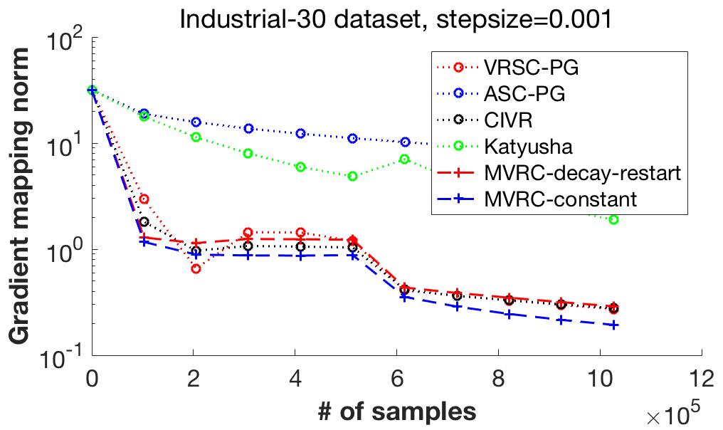
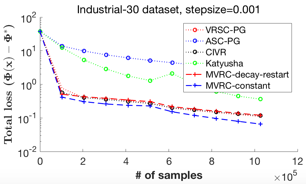
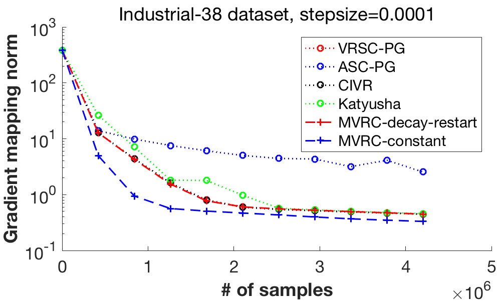
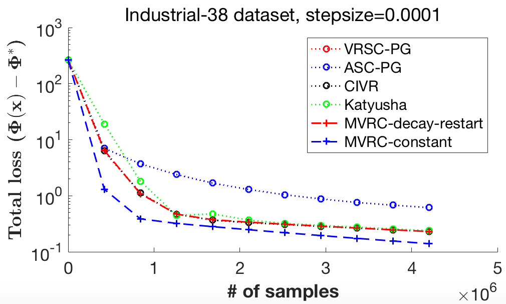
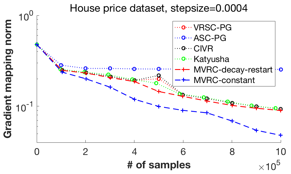
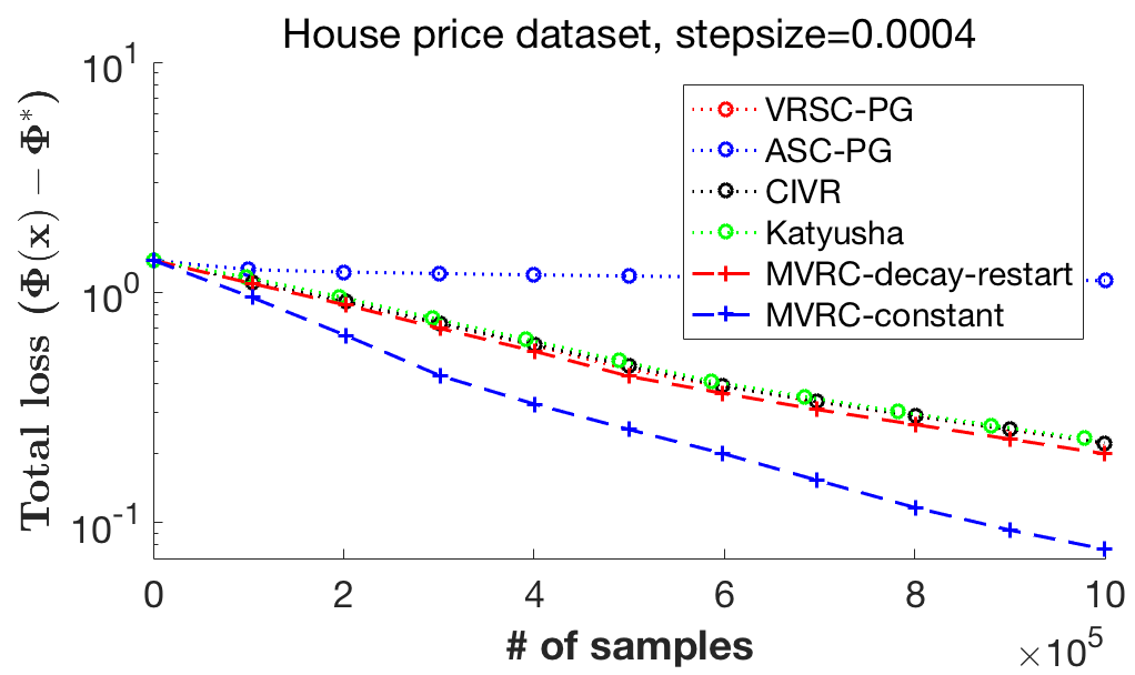
Figure 1: Columns 1-2: Comparison of composition optimization algorithms in solving risk-averse portfolio optimization problems. Column 3: Comparison of composition optimization algorithms in solving nonconvex and nonsmooth sparse additive models.

5.1 Risk-averse Portfolio Optimization

We consider the risk-averse portfolio optimization problem as elaborated in Appendix A. In specific, we set $\lambda=0.2$ in item 1 and add an $\ell_{1}$-regularizer $r(x)=0.01\|x\|_{1}$ to the objective function. We specify the values of $\{R_{i}\}_{i=1}^{n}$ using two industrial portfolio datasets from the Keneth R. French Data Library , which have dimension $d=30$ and $d=38$, respectively. As in (Zhang & Xiao, 2019c), we select the most recent $n=24452,10000$ days from the two datasets, respectively. We implement all the algorithms using the same initialization point, batch size 256 and learning rate $\eta=10^{-3},10^{-4}$ respectively for the two datasets. For variance-reduced algorithms, we set each epoch to include $J=\lceil n/256\rceil$ inner iterations. For ASC-PG, we set $\alpha_{t}=0.0001t^{-5/9}$, $\beta_{t}=t^{-4/9}$ as used by (Zhang & Xiao, 2019c), whereas for Katyusha (Xu & Xu, 2019) we set $\tau_{1}=\tau_{2}=0.4$, $L=1/(3\eta)$, $\alpha=\eta$, $\theta=1/(12J)$. For our MVRC (Algorithm 1), we consider two settings: 1) diminishing momentum with restart, which chooses $\alpha_{t}=\frac{2}{t+1}$, $\beta_{t}\equiv\eta$, $\lambda_{t}=\frac{t+3}{t+1}\eta$, where $t$ is reset to 0 and $y_{t},z_{t}$ are reset to $x_{t}$ after each epoch; and 2) constant momentum, which chooses $\alpha_{t}\equiv 0.8$, $\beta_{t}\equiv\eta$, $\lambda_{t}\equiv 1.8\eta$.

Figure 1 (Columns 1 & 2) presents the convergence curves of these algorithms on both datasets with regard to the gradient mapping norm (top row) and function value gap (bottom row). It can be seen that our MVRC with constant momentum (shown as “MVRC-constant”) achieves the fastest convergence among all the algorithms and is significantly faster than the Katyusha composition optimization algorithm. Also, the convergence of our MVRC with diminishing momentum and restart (shown as “MVRC-decay-restart”) is comparable to that of CIVR and VRSC-PG, and is faster than ASC-PG.

5.2 Nonconvex & Nonsmooth Sparse Additive Model

We further test these algorithms via solving the sparse additive model as introduced in Appendix A, where we use linear model $h_{j}(x_{j})=\theta_{j}x_{j}$ and set $\lambda=1$. In particular, we adopt a modified nonconvex and nonsmooth problem (4) where the prediction is obtained via the nonlinear model ${\widehat{y}_{i}}=|\sum_{j=1}^{d}h_{j}(x_{ij})|$ and the objective function is further penalized by an $\ell_{1}$ regularization $r(x)=0.001\|x\|_{1}$. We use the US house price data that consists of 5000 houses with their prices being approximated via linear combinations of averge income, age, number of rooms and population of a house per area. The price serves as the output and these four features with other 96 random Gaussian features serve as the input. To promote sparsity, all the coefficients of the Gaussian features are set to zero. All the algorithms use the same initialization point, learning rate $\eta=0.004$, batch sizes 10 and 70 for $f$ and $g$, respectively, epoch length $J=140$. For ASC-PG, we set $\alpha_{t}=0.004t^{-5/9}$, $\beta_{t}=2t^{-4/9}$. The other hyper-parameters of ASC-PG, Katyusha and our MVRC are the same as those specified in the previous subsection.

Figure 1 (Column 3) presents the convergence curves of these algorithms with regard to the gradient mapping norm (top right) and function value gap (bottom right). It can be seen that our MVRC with constant momentum (shown as “MVRC-constant”) converges significantly faster than the other algorithms, in particular, faster than the Katyusha composition optimization algorithm. Also, the convergence of our MVRC with diminishing momentum and restart (shown as “MVRC-decay-restart”) is comparable to that of CIVR, VRSC-PG and Katyusha. These experiments demonstrate that our MVRC provides significant practical acceleration to nonconvex stochastic composition optimization.

6 Conclusion

In this paper, we develop momentum with variance reduction schemes for solving both finite-sum and online composition optimization problems and provide a comprehensive sample complexity analysis in nonconvex optimization. Our MVRC achieves the state-of-the-art near-optimal sample complexities and attains a linear convergence under the gradient dominant condition. We empirically demonstrate that MVRC with constant momentum outperforms all the other existing stochastic algorithms for composition optimization. In the future work, it is interesting to study the convergence guarantee for MVRC in solving more complex nonconvex problems such the model-agnostic meta-learning and reinforcement learning.

Supplemental Materials

Appendix A Elaboration of Compositional Structure in ML Applications

1. Risk-averse portfolio optimization (Zhang & Xiao, 2019c):
   In this problem, we need to decide the amount of investment $x\in\mathbb{R}^{d}$ that involves $d$ assets to maximize the following total expected return penalized by the risk (i.e., the variance of the return)

   $$\min_{x\in\mathbb{R}^{d}}\mathbb{E}_{\xi}h_{\xi}(x)-\lambda\text{var}_{\xi}h_{\xi}(x),$$ (15)

   where $h_{\xi}(x)$ is the return at a random time $\xi$. Furthermore, suppose $R_{\xi}\in\mathbb{R}^{d}$ records the return per unit investment for each of the $d$ assets, such that $h_{\xi}(x)=R_{\xi}^{\top}x$, and the time $\xi$ is uniformly obtained from $1,2,\ldots,n$. Then, the objective function (15) can be reformulated as the composition problem $(\Sigma^{1})$ with

   $$f(y_{1},y_{2})=-y_{1}-\lambda(y_{1}^{2}-y_{2})$$

   $$g_{i}(x)=[h_{i}(x),h_{i}^{2}(x)]=[R_{i}^{\top}x,(R_{i}^{\top}x)^{2}].$$ (16)

2. Linear value function approximation in reinforcement learning (Zhang & Xiao, 2019c):
   Consider a Markov decision process (MDP) with finite state space $\mathcal{S}=\{1,\ldots,S\}$, transition probability matrix $P^{\pi}$ associated with a certain policy $\pi$, and a random reward $R_{i,j}$ obtained after going from state $i$ to state $j$. Then the value function $V^{\pi}:\mathcal{S}\to\mathbb{R}$ must satisfy the Bellman equation:

   $$V^{\pi}(i)=\sum_{j=1}^{S}P_{i,j}^{\pi}\left(R_{i,j}+\gamma V^{\pi}(j)\right)$$ (17)

   When the number of states $S$ is large, the value function $V^{\pi}$ can be approximated by some function $\widetilde{V}^{\pi}_{i}(w)$ parameterized by $w\in\mathbb{R}^{d}$ to alleviate the computation burden. A simple example is the linear function approximation $\widetilde{V}_{i}^{\pi}(w)=\Phi_{i}^{\top}w$, where $\Phi_{i}\in\mathbb{R}^{d}$ is fixed. The goal of the value function approximation is to learn the parameter $w$ to minimize the following mean squared error

   $$\min_{w\in\mathbb{R}^{d}}F(w):= \frac{1}{S}\sum_{i=1}^{S}\Big{[}\widetilde{V}^{\pi}_{i}(w)-\sum_{j=1}^{S}P_{i,j}^{\pi}(R_{i,j}+\gamma\widetilde{V}^{\pi}_{j}(w))\Big{]}^{2},$$ (18)

   which can be reformulated as the problem $(\mathbb{E}^{2})$ with

   $$\eta=i\mathop{\sim}\limits^{\text{uniform}}\{1,\ldots,S\},\mathbb{P}(\xi=j|\eta=i)=P_{i,j}^{\pi},$$

   $$g_{\xi}(w)=[\widetilde{V}_{i}^{\pi}(w),R_{i,\xi}+\gamma\widetilde{V}^{\pi}_{\xi}(w)],$$

   $$f_{i}(y_{1},y_{2})=(y_{1}-y_{2})^{2},$$ (19)

   or the problem $(\mathbb{E}^{1})$ with

   $$q_{i}^{\pi}(w)=\mathbb{E}(w)=\mathbb{E}_{\xi}[R_{i,\xi}+\gamma\widetilde{V}^{\pi}_{\xi}(w)|i]~{}\text{with}~{}\mathbb{P}(\xi=j|i)=P_{i,j}^{\pi},$$

   $$g(w)=[\widetilde{V}_{1}^{\pi}(w),\ldots,\widetilde{V}_{S}^{\pi}(w),q_{1}^{\pi}(w),\ldots,q_{S}^{\pi}(w)],$$

   $$f(y_{1},\ldots,y_{S},z_{1},\ldots,z_{S})=\frac{1}{S}\sum_{k=1}^{S}(y_{k}-z_{k})^{2}.$$ (20)

3. Stochastic neighbor embedding (SNE) (Liu et al., 2017):
   SNE aims at dimension reduction while keeping the original metric among data points as much as possible from a probabilistic view (Hinton & Roweis, 2003). Specifically, for a set of given data points $z_{1},\ldots,z_{n}\in\mathbb{R}^{d}$, a data point $z_{k}$ has probability

   $$p_{i|k}=\frac{s(z_{i},z_{k})}{\sum_{j\neq k}s(z_{j},z_{k})}$$ (21)

   to select $x_{i}(i\neq k)$ as its neighbor, where $s(x_{i},x_{j})$ is the similarity measure between $x_{i}$ and $x_{j}$, e.g., the Gaussian form $s(x_{i},x_{j})=\exp\left(-\|x_{i}-x_{j}\|^{2}/(2\sigma_{i}^{2})\right)$. We want to find a $p$-dim ($p<d$) representation $x_{1},\ldots,x_{n}\in\mathbb{R}^{p}$ such that its neighbor selection probability

   $$q_{i|k}=\frac{s(x_{i},x_{k})}{\sum_{j\neq k}s(x_{j},x_{k})}$$ (22)

   is close to the probability (21). A natural way is to minimize the KL divergence $\text{KL}(p_{i|k},q_{i|k})=\sum_{i=1}^{n}\sum_{k=1}^{n}p_{i|k}\log(p_{i|k}/q_{i|k})$, which is equivalent to minimize

   $$\Phi(x)= -\frac{1}{n^{2}}\sum_{i=1}^{n}\sum_{k=1}^{n}p_{i|k}\log q_{i|k},$$

   $$= \frac{1}{n^{2}}\sum_{i=1}^{n}\sum_{k=1}^{n}p_{i|k}\Big{[}\log\Big{(}\frac{1}{n}\sum_{j=1}^{n}s\left(x_{j},x_{k}\right)-\frac{1}{n}s\left(x_{k},x_{k}\right)\Big{)}-\log\Big{(}\frac{1}{n}s\left(x_{i},x_{k}\right)\Big{)}\Big{]},$$ (23)

   where $x=[x_{1},\ldots,x_{n}]\in\mathbb{R}^{np}.$ This problem can be reformulated as the problem $(\Sigma^{2})$ with

   $$\Phi(x)=\frac{1}{n^{2}}\sum_{i=1}^{n}\sum_{k=1}^{n}f_{i,k}\left[\frac{1}{n}\sum_{j=1}^{n}g_{j}(x)\right],$$ (24)

   where

   $$g_{j}(x)= \Big{[}x_{1},x_{2},\ldots,x_{n},s(x_{j},x_{1})-\frac{1}{n}s(x_{1},x_{1}),\ldots,s(x_{j},x_{n})-\frac{1}{n}s(x_{n},x_{n})\Big{]},$$ (25)

   $$f_{i,k}(w)=p_{i|k}\Big{[}\log w_{n+k}-\log\Big{(}\frac{1}{n}s(w_{i},w_{k})\Big{)}\Big{]}.$$ (26)

4. Sparse additive model (SpAM) (Wang et al., 2017):
   SpAM is an important model for nonparametric regression where the input vector $x_{i}=(x_{i1},\ldots,x_{id})^{\top}\in\mathbb{R}^{d}$ is high-dimensional. The true output is $y_{i}\in\mathbb{R}$ and the corresponding model prediction is $\widehat{y}_{i}=\sum_{j=1}^{d}h_{j}(x_{ij})$, where $h_{j}:\mathbb{R}\to\mathbb{R}$ is selected from a certain function family $\mathcal{H}_{j}$. The object is to minimize the following penalized mean squared error

   $$\min_{h_{j}\in\mathcal{H}_{j},j=1\ldots,d} \frac{1}{n}\sum_{i=1}^{n}\Big{[}y_{i}-\sum_{j=1}^{d}h_{j}\left(x_{ij}\right)\Big{]}^{2}+\lambda\sum_{j=1}^{d}\sqrt{\frac{1}{n}\sum_{i=1}^{n}h_{j}^{2}\left(x_{ij}\right)},$$ (27)

   (Huang et al., 2010) showed some good statistical properties of SpAM. To use an efficient stochastic optimizer, the objective function (27) is further reformulated as the problem $(\Sigma^{2})$ with

   $$g_{i}(h_{1},\ldots,h_{d})=\Big{[}\Big{(}y_{i}-\sum_{j=1}^{d}h_{j}\left(x_{ij}\right)\Big{)}^{2},h_{1}(x_{i1})^{2},\ldots,h_{d}(x_{id})^{2}\Big{]}^{\top},$$

   $$f_{k}(y)=\left\{\begin{gathered}{y_{1}};k=1\hfill\\ \sqrt{|{y_{k}}|};2\leqslant k\leqslant d+1\hfill\\ \end{gathered}\right..$$ (31)

   In our experiment in Section 5.2, we adopt a nonconvex and nonsmooth modification of the SpAM, which is also formulated as the problem $(\Sigma^{2})$ with

   $$g_{i}(h_{1},\ldots,h_{d})=\Big{[}\Big{(}y_{i}-\Big{|}\sum_{j=1}^{d}h_{j}\left(x_{ij}\right)\Big{|}\Big{)}^{2},h_{1}(x_{i1})^{2},\ldots,h_{d}(x_{id})^{2}\Big{]}^{\top},$$

   $$f_{1}(y)=y_{1},$$

   $$f_{k}(y)=\left\{\begin{gathered}\sqrt{|{y_{k}}|};|y_{k}|\geq 1\hfill\\ 1.75y_{k}^{2}-0.75y_{k}^{4};|y_{k}|<1\hfill\\ \end{gathered}\right.;2\leqslant k\leqslant d+1$$ (35)

   $$r(x)=\mu\|x\|_{1},$$ (36)

   where the prediction ${\widehat{y}_{i}}=|\sum_{j=1}^{d}h_{j}(x_{ij})|$ is nonlinear and nonnegative, and the square root function in $[-1,1]$ is modified to ensure bounded derivative.

Appendix B Auxiliary Lemmas for Proving 1

The following Lemma 1 originates from the Lemma 1 of (Zhang & Xiao, 2019c), and we present it for completeness.

Lemma 1.

Let Assumptions 1 and 2 hold and apply Algorithm 1 to solve the problems $(\Sigma^{1})$ and $(\mathbb{E}^{1})$. Then, the variance of the stochastic gradient satisfies

$$\mathbb{E} \left\|\widetilde{\nabla}F\left(z_{t}\right)-\nabla F\left(z_{t}\right)\right\|^{2}\leq\frac{\sigma_{0}^{2}}{|\mathcal{A}_{\tau\left\lfloor t/\tau\right\rfloor}|}+G_{0}\sum_{s=\tau\lfloor t/\tau\rfloor+1}^{t}\frac{1}{|\mathcal{A}_{s}|}\mathbb{E}\left\|z_{s}-z_{s-1}\right\|^{2},$$ (37)

where

$$G_{0}:= 2\left(l_{g}^{4}L_{f}^{2}+l_{f}^{2}L_{g}^{2}\right),$$

$$\sigma_{0}^{2}:= \left\{\begin{gathered}0;\text{For the problem }(\Sigma^{1})\hfill\\ 2\left(l_{g}^{2}L_{f}^{2}\sigma_{g}^{2}+l_{f}^{2}\sigma_{g^{\prime}}^{2}\right);\text{For the problem }(\mathbb{E}^{1})\hfill\\ \end{gathered}\right.$$ (41)

Note that when $t=m\tau$ for some positive integer $m$, the summation becomes $\sum_{s=m\tau+1}^{m\tau}$, which is 0 by default.

Lemma 2.

Implement Algorithm 1 with $\alpha_{t}=\frac{2}{t+1},\beta_{t}\equiv\beta,\beta\leq\lambda_{t}\leq(1+\alpha_{t})\beta$ to solve the problems $(\Sigma^{1})$ and $(\mathbb{E}^{1})$. Then, the generated sequences $\{x_{t},y_{t},z_{t}\}$ satisfy

$$y_{t}-x_{t}=-\Gamma_{t}\sum_{s=1}^{t}\frac{\lambda_{s-1}-\beta}{\Gamma_{s}\lambda_{s-1}}(x_{s}-x_{s-1}),$$ (42)

$$\left\|y_{t}-x_{t}\right\|^{2}\leq\Gamma_{t}\sum_{s=1}^{t}\frac{(\lambda_{s-1}-\beta)^{2}}{\alpha_{s}\Gamma_{s}\lambda_{s-1}^{2}}\left\|x_{s}-x_{s-1}\right\|^{2},$$ (43)

$$\left\|z_{t+1}-z_{t}\right\|^{2}\leq\frac{2\beta_{t}^{2}}{\lambda_{t}^{2}}\left\|x_{t+1}-x_{t}\right\|^{2}+2\alpha_{t+2}^{2}\Gamma_{t+1}\sum_{s=1}^{t+1}\frac{\left(\lambda_{s-1}-\beta_{s-1}\right)^{2}}{\alpha_{s}\Gamma_{s}\lambda_{s-1}^{2}}\left\|x_{s}-x_{s-1}\right\|^{2},$$ (44)

where $\Gamma_{t}=\frac{2}{t(t+1)}$. When $t=0$, the summation $\sum_{t=1}^{0}$ is 0 by default.

Proof.

Based on the update rules in Algorithm 1,

$$y_{t+1}-x_{t+1}= z_{t}+\frac{\beta_{t}}{\lambda_{t}}(x_{t+1}-x_{t})-x_{t+1}$$

$$= \left(1-\alpha_{t+1}\right)y_{t}+\alpha_{t+1}x_{t}+\frac{\beta_{t}}{\lambda_{t}}(x_{t+1}-x_{t})-x_{t+1}$$

$$= \left(1-\alpha_{t+1}\right)(y_{t}-x_{t})+\left(\frac{\beta_{t}}{\lambda_{t}}-1\right)(x_{t+1}-x_{t}).$$

Taking the above equality as a difference equation about $y_{t}-x_{t}$ with initial condition $y_{0}-x_{0}=0$, it can be verified that Eq. (42) is the solution. Hence,

$$\|y_{t}-x_{t}\|^{2}= \left\|\Gamma_{t}\sum_{s=1}^{t}\frac{\lambda_{s-1}-\beta}{\Gamma_{s}\lambda_{s-1}}(x_{s}-x_{s-1})\right\|^{2}$$

$$= \left\|\sum_{s=1}^{t}\frac{\Gamma_{t}\alpha_{s}}{\Gamma_{s}}\frac{\lambda_{s-1}-\beta}{\alpha_{s}\lambda_{s-1}}(x_{s}-x_{s-1})\right\|^{2}$$

$$\leq \sum_{s=1}^{t}\frac{\Gamma_{t}\alpha_{s}}{\Gamma_{s}}\left\|\frac{\lambda_{s-1}-\beta}{\alpha_{s}\lambda_{s-1}}(x_{s}-x_{s-1})\right\|^{2}$$

$$= \sum_{s=1}^{t}\frac{\Gamma_{t}(\lambda_{s-1}-\beta)^{2}}{\Gamma_{s}\alpha_{s}\lambda_{s-1}^{2}}\left\|x_{s}-x_{s-1}\right\|^{2},$$

where $\leq$ applies Jensen’s inequality to the convex function $\|\bullet\|^{2}$ with $\sum_{s=1}^{t}\frac{\Gamma_{t}\alpha_{s}}{\Gamma_{s}}=1$. This proves Eq. (43).

It can be derived from the update rules in Algorithm 1 that $z_{t+1}-z_{t}=\beta_{t}(x_{t+1}-x_{t})/\lambda_{t}-\alpha_{t+2}(y_{t+1}-x_{t+1})$. Hence,

$$\|z_{t+1}-z_{t}\|^{2}= \left\|\frac{\beta_{t}}{\lambda_{t}}(x_{t+1}-x_{t})-\alpha_{t+2}(y_{t+1}-x_{t+1})\right\|^{2}$$

$$\leq 2\left\|\frac{\beta_{t}}{\lambda_{t}}(x_{t+1}-x_{t})\right\|^{2}+2\alpha_{t+2}^{2}\left\|y_{t+1}-x_{t+1}\right\|^{2}$$

$$\leq \frac{2\beta_{t}^{2}}{\lambda_{t}^{2}}\left\|x_{t+1}-x_{t}\right\|^{2}+2\alpha_{t+2}^{2}\Gamma_{t+1}\sum_{s=1}^{t+1}\frac{(\lambda_{s-1}-\beta)^{2}}{\alpha_{s}\Gamma_{s}\lambda_{s-1}^{2}}\left\|x_{s}-x_{s-1}\right\|^{2},$$

which proves Eq. (44). ∎

Appendix C Proof of 1

Since $x_{t+1}$ is the minimizer of the function $\widetilde{r}(x):=r(x)+\frac{1}{2\lambda_{t}}\|x-x_{t}+\lambda_{t}{\widetilde{\nabla}F}(z_{t})\|^{2}$, which is $\lambda_{t}^{-1}$-strongly convex as $r$ is convex, we have

$$\widetilde{r}(x_{t})\geq\widetilde{r}(x_{t+1})+\frac{1}{2\lambda_{t}}\|x_{t+1}-x_{t}\|^{2}$$

$$\Rightarrow r(x_{t})+\frac{\lambda_{t}}{2}\|{\widetilde{\nabla}F}(z_{t})\|^{2}\geq r(x_{t+1})+\frac{1}{2\lambda_{t}}\|x_{t+1}-x_{t}+\lambda_{t}{\widetilde{\nabla}F}(z_{t})\|^{2}+\frac{1}{2\lambda_{t}}\|x_{t+1}-x_{t}\|^{2}$$

$$\Rightarrow r(x_{t+1})-r(x_{t})\leq-\frac{1}{\lambda_{t}}\|x_{t+1}-x_{t}\|^{2}-\left<{\widetilde{\nabla}F}(z_{t}),x_{t+1}-x_{t}\right>.$$ (45)

Since $\nabla F$ is $L_{F}$-Lipschitz, we obtain that

$$F(x_{t+1})-F(x_{t})\leq\left<\nabla F(x_{t}),x_{t+1}-x_{t}\right>+\frac{L_{F}}{2}\|x_{t+1}-x_{t}\|^{2}.$$ (46)

Adding up Eqs. (C)$\&$(46) and taking expectation, we further obtain that

$$\mathbb{E}\Phi(x_{t+1})-\mathbb{E}\Phi(x_{t})\leq \mathbb{E}\left<\nabla F(x_{t})-{\widetilde{\nabla}F}(z_{t}),x_{t+1}-x_{t}\right>+\left(\frac{L_{F}}{2}-\frac{1}{\lambda_{t}}\right)\mathbb{E}\|x_{t+1}-x_{t}\|^{2}$$

$$= \mathbb{E}\left<\nabla F(z_{t})-{\widetilde{\nabla}F}(z_{t}),x_{t+1}-x_{t}\right>+\mathbb{E}\left<\nabla F(x_{t})-\nabla F(z_{t}),x_{t+1}-x_{t}\right>$$

$$+\left(\frac{L_{F}}{2}-\frac{1}{\lambda_{t}}\right)\mathbb{E}\|x_{t+1}-x_{t}\|^{2}$$

$$\leq \mathbb{E}\left(\left\|\nabla F(z_{t})-{\widetilde{\nabla}F}(z_{t})\right\|\left\|x_{t+1}-x_{t}\right\|\right)+\mathbb{E}\left(\left\|\nabla F(x_{t})-\nabla F(z_{t})\right\|\left\|x_{t+1}-x_{t}\right\|\right)$$

$$+\left(\frac{L_{F}}{2}-\frac{1}{\lambda_{t}}\right)\mathbb{E}\|x_{t+1}-x_{t}\|^{2}$$

$$\leq \frac{\lambda_{t}}{2}\mathbb{E}\left\|\nabla F(z_{t})-{\widetilde{\nabla}F}(z_{t})\right\|^{2}+\frac{1}{2\lambda_{t}}\mathbb{E}\left\|x_{t+1}-x_{t}\right\|^{2}$$

$$+L_{F}\mathbb{E}\left(\left\|x_{t}-z_{t}\right\|\left\|x_{t+1}-x_{t}\right\|\right)+\left(\frac{L_{F}}{2}-\frac{1}{\lambda_{t}}\right)\mathbb{E}\|x_{t+1}-x_{t}\|^{2}$$

$$\leq \frac{\lambda_{t}}{2}\mathbb{E}\left\|\nabla F(z_{t})-{\widetilde{\nabla}F}(z_{t})\right\|^{2}+\frac{1}{2\lambda_{t}}\mathbb{E}\left\|x_{t+1}-x_{t}\right\|^{2}$$

$$+L_{F}(1-\alpha_{t+1})\mathbb{E}\left(\left\|y_{t}-x_{t}\right\|\left\|x_{t+1}-x_{t}\right\|\right)+\left(\frac{L_{F}}{2}-\frac{1}{\lambda_{t}}\right)\mathbb{E}\|x_{t+1}-x_{t}\|^{2}$$

$$\leq \frac{\lambda_{t}}{2}\mathbb{E}\left\|\nabla F(z_{t})-{\widetilde{\nabla}F}(z_{t})\right\|^{2}+\frac{1}{2\lambda_{t}}\mathbb{E}\left\|x_{t+1}-x_{t}\right\|^{2}$$

$$+\frac{L_{F}}{2}\mathbb{E}\left\|y_{t}-x_{t}\right\|^{2}+\frac{L_{F}}{2}\mathbb{E}\left\|x_{t+1}-x_{t}\right\|^{2}+\left(\frac{L_{F}}{2}-\frac{1}{\lambda_{t}}\right)\mathbb{E}\|x_{t+1}-x_{t}\|^{2}$$

$$\leq \frac{\lambda_{t}}{2}\mathbb{E}\left\|\nabla F(z_{t})-{\widetilde{\nabla}F}(z_{t})\right\|^{2}+\left(L_{F}-\frac{1}{2\lambda_{t}}\right)\mathbb{E}\|x_{t+1}-x_{t}\|^{2}$$

$$+\frac{L_{F}\Gamma_{t}}{2}\sum_{s=1}^{t}\frac{(\lambda_{s-1}-\beta)^{2}}{\alpha_{s}\Gamma_{s}\lambda_{s-1}^{2}}\left\|x_{s}-x_{s-1}\right\|^{2},$$ (47)

where the last inequality uses Eq. (43). Telescoping the above inequality over $t$ from $0$ to $T-1$ yields that

$$\mathbb{E}\Phi(x_{T})-\Phi(x_{0})\leq \sum_{t=0}^{T-1}\frac{\lambda_{t}}{2}\mathbb{E}\left\|\nabla F(z_{t})-{\widetilde{\nabla}F}(z_{t})\right\|^{2}+\sum_{t=0}^{T-1}\left(L_{F}-\frac{1}{2\lambda_{t}}\right)\mathbb{E}\|x_{t+1}-x_{t}\|^{2}$$

$$+\sum_{t=0}^{T-1}\frac{L_{F}\Gamma_{t}}{2}\sum_{s=1}^{t}\frac{(\lambda_{s-1}-\beta)^{2}}{\alpha_{s}\Gamma_{s}\lambda_{s-1}^{2}}\left\|x_{s}-x_{s-1}\right\|^{2}$$

$$\stackrel{{\scriptstyle(i)}}{{\leq}} \sum_{t=0}^{T-1}\frac{\lambda_{t}}{2}\left[G_{0}\sum_{s=\tau\left\lfloor t/\tau\right\rfloor+1}^{t}\frac{1}{|\mathcal{A}_{s}|}\mathbb{E}\left\|z_{s}-z_{s-1}\right\|^{2}+\frac{\sigma_{0}^{2}}{|\mathcal{A}_{\tau\left\lfloor t/\tau\right\rfloor}|}\right]$$

$$+\sum_{t=0}^{T-1}\left(L_{F}-\frac{1}{2\lambda_{t}}\right)\mathbb{E}\|x_{t+1}-x_{t}\|^{2}$$

$$+\frac{L_{F}}{2}\sum_{s=1}^{T-1}\frac{(\lambda_{s-1}-\beta)^{2}}{\alpha_{s}\Gamma_{s}\lambda_{s-1}^{2}}\left(\sum_{t=s}^{T-1}\Gamma_{t}\right)\mathbb{E}\left\|x_{s}-x_{s-1}\right\|^{2}$$

$$\stackrel{{\scriptstyle(ii)}}{{=}} \frac{G_{0}}{2}\sum_{s=1}^{T-1}\frac{1}{|\mathcal{A}_{s}|}\mathbb{E}\left\|z_{s}-z_{s-1}\right\|^{2}\sum_{t=s}^{\min\left(\tau\left\lfloor\frac{s-1}{\tau}\right\rfloor+\tau-1,T-1\right)}\lambda_{t}+\frac{\sigma_{0}^{2}}{2}\sum_{t=0}^{T-1}\frac{\lambda_{t}}{|\mathcal{A}_{\tau\left\lfloor t/\tau\right\rfloor}|}$$

$$+\sum_{t=0}^{T-1}\left(L_{F}-\frac{1}{2\lambda_{t}}\right)\mathbb{E}\|x_{t+1}-x_{t}\|^{2}$$

$$+L_{F}\sum_{s=1}^{T-1}\frac{(\lambda_{s-1}-\beta)^{2}}{\alpha_{s}\Gamma_{s}\lambda_{s-1}^{2}}\sum_{t=s}^{T-1}\left(\frac{1}{t}-\frac{1}{t+1}\right)\mathbb{E}\left\|x_{s}-x_{s-1}\right\|^{2}$$

$$\stackrel{{\scriptstyle(iii)}}{{\leq}} \frac{G_{0}}{2}\sum_{s=1}^{T-1}\frac{1}{\tau}\mathbb{E}\|z_{s}-z_{s-1}\|^{2}\left(\tau\left\lfloor\frac{s-1}{\tau}\right\rfloor+\tau-1-(s-1)\right)(2\beta)$$

$$+\frac{T\beta\sigma_{0}^{2}}{|\mathcal{A}_{0}|}+\sum_{t=0}^{T-1}\left(L_{F}-\frac{1}{4\beta}\right)\mathbb{E}\|x_{t+1}-x_{t}\|^{2}$$

$$+\frac{L_{F}}{4}\sum_{s=1}^{T-1}s(s+1)^{2}\left(\frac{\alpha_{s-1}}{1+\alpha_{s-1}}\right)^{2}\mathbb{E}\|x_{s}-x_{s-1}\|^{2}\left(\frac{1}{s}-\frac{1}{T}\right)$$

$$\stackrel{{\scriptstyle(iv)}}{{\leq}} \beta G_{0}\sum_{s=1}^{T-1}\left[\frac{2\beta^{2}}{\lambda_{s-1}^{2}}\mathbb{E}\left\|x_{s}-x_{s-1}\right\|^{2}+2\alpha_{s+1}^{2}\Gamma_{s}\sum_{t=1}^{s}\frac{(\lambda_{t-1}-\beta)^{2}}{\alpha_{t}\Gamma_{t}\lambda_{t-1}^{2}}\mathbb{E}\left\|x_{t}-x_{t-1}\right\|^{2}\right]$$

$$+\frac{T\beta\sigma_{0}^{2}}{|\mathcal{A}_{0}|}+\sum_{t=0}^{T-1}\left(L_{F}-\frac{1}{4\beta}\right)\mathbb{E}\|x_{t+1}-x_{t}\|^{2}$$

$$+\frac{L_{F}}{4}\sum_{s=1}^{T-1}s(s+1)^{2}\frac{4}{(s+2)^{2}}\mathbb{E}\|x_{s}-x_{s-1}\|^{2}\left(\frac{1}{s}-\frac{1}{T}\right)$$

$$\stackrel{{\scriptstyle(v)}}{{\leq}} 2\beta G_{0}\sum_{s=1}^{T-1}\mathbb{E}\left\|x_{s}-x_{s-1}\right\|^{2}$$

$$+2\beta G_{0}\sum_{t=1}^{T-1}\sum_{s=t}^{T-1}\frac{4}{(s+2)^{2}}\frac{2}{s(s+1)}\frac{t+1}{2}\frac{t(t+1)}{2}\left(\frac{\alpha_{t-1}}{1+\alpha_{t-1}}\right)^{2}\mathbb{E}\left\|x_{t}-x_{t-1}\right\|^{2}$$

$$+\frac{T\beta\sigma_{0}^{2}}{|\mathcal{A}_{0}|}+\sum_{t=0}^{T-1}\left(L_{F}-\frac{1}{4\beta}\right)\mathbb{E}\|x_{t+1}-x_{t}\|^{2}+L_{F}\sum_{t=0}^{T-2}\mathbb{E}\|x_{t+1}-x_{t}\|^{2}$$

$$\stackrel{{\scriptstyle(vi)}}{{\leq}} 2\beta G_{0}\sum_{t=0}^{T-2}\mathbb{E}\left\|x_{t+1}-x_{t}\right\|^{2}+\beta G_{0}\sum_{t=1}^{T-1}(t+1)\frac{4}{(t+2)^{2}}\mathbb{E}\left\|x_{t}-x_{t-1}\right\|^{2}$$

$$+\frac{T\beta\sigma_{0}^{2}}{|\mathcal{A}_{0}|}+\sum_{t=0}^{T-1}\left(2L_{F}-\frac{1}{4\beta}\right)\mathbb{E}\|x_{t+1}-x_{t}\|^{2}$$

$$\leq \frac{T\beta\sigma_{0}^{2}}{|\mathcal{A}_{0}|}+\left(3\beta G_{0}+2L_{F}-\frac{1}{4\beta}\right)\sum_{t=0}^{T-1}\mathbb{E}\|x_{t+1}-x_{t}\|^{2},$$ (48)

where (i) follows from Lemma 1 and switches the last two summations, (ii) switches the first two summations, (iii) uses the hyperparameter choices that $\beta\leq\lambda_{t}\leq(1+\alpha_{t})\beta\leq 2\beta$, $|\mathcal{A}_{t}|\geq\tau$ and $|\mathcal{A}_{m\tau}|\equiv|\mathcal{A}_{0}|(m\in\mathbb{N})$, (iv) uses Eq. (44), $\frac{1}{\tau}\left(\tau\left\lfloor\frac{s-1}{\tau}\right\rfloor+\tau-1-(s-1)\right)\leq 1$ and $\beta\leq\lambda_{t}\leq(1+\alpha_{t})\beta\leq 2\beta$, (v) switches the first two summations and replaces $s$ with $t+1$ in the last summation, (vi) uses the following inequality

$$\sum_{s=t}^{T-1}\frac{1}{s(s+1)(s+2)^{2}}= \frac{1}{2}\sum_{s=t}^{T-1}\left(\frac{1}{s}-\frac{1}{s+2}\right)\left(\frac{1}{s+1}-\frac{1}{s+2}\right)$$

$$= \frac{1}{2}\sum_{s=t}^{T-1}\left[\left(\frac{1}{s}-\frac{1}{s+1}\right)-\left(\frac{1}{s+1}-\frac{1}{s+2}\right)-\frac{1}{2}\left(\frac{1}{s}-\frac{1}{s+2}\right)+\frac{1}{(s+2)^{2}}\right]$$

$$= \frac{1}{2}\left[\left(\frac{1}{t}-\frac{1}{T}\right)-\left(\frac{1}{t+1}-\frac{1}{T+1}\right)-\frac{1}{2}\left(\frac{1}{t}+\frac{1}{t+1}-\frac{1}{T}-\frac{1}{T+1}\right)\right.$$

$$+\left.\int_{t-1}^{T-1}\frac{ds}{(s+2)^{2}}\right]$$

$$= \frac{1}{4t}-\frac{3}{4(t+1)}-\frac{1}{4T}+\frac{3}{4(T+1)}+\frac{1}{2}\left(\frac{1}{t+1}-\frac{1}{T+1}\right)$$

$$\leq \frac{1}{4t(t+1)}.$$ (49)

Let $3\beta G_{0}+2L_{F}-\frac{1}{4\beta}\leq-\frac{1}{8\beta}$, which together with $\beta>0$ implies $0<\beta\leq\frac{1}{2\sqrt{16L_{F}^{2}+6G_{0}}+8L_{F}}$. Then Eq. (C) further indicates that

$$\sum_{t=0}^{T-1}\mathbb{E}\|x_{t+1}-x_{t}\|^{2}\leq\frac{8T\beta^{2}\sigma_{0}^{2}}{|\mathcal{A}_{0}|}+8\beta\left[\Phi\left(x_{0}\right)-\mathbb{E}\Phi(x_{T})\right].$$ (50)

Therefore, let $\zeta$ be sampled from $\{0,...,T-1\}$ uniformly at random, we obtain that

$$\mathbb{E}\|{\mathcal{G}}_{\lambda_{\zeta}}(z_{\zeta})\|^{2}= \frac{1}{T}\sum_{t=0}^{T-1}\mathbb{E}\|{\mathcal{G}}_{\lambda_{t}}(z_{t})\|^{2}$$

$$\stackrel{{\scriptstyle(i)}}{{=}} \frac{1}{T}\sum_{t=0}^{T-1}\lambda_{t}^{-2}\mathbb{E}\left\|z_{t}-\operatorname{prox}_{\lambda_{t}r}\left[z_{t}-\lambda_{t}\nabla F(z_{t})\right]\right\|^{2}$$

$$\stackrel{{\scriptstyle(ii)}}{{=}} \frac{9}{T}\sum_{t=0}^{T-1}\lambda_{t}^{-2}\mathbb{E}\left\|\frac{1}{3}(z_{t}-x_{t})+\frac{1}{3}(x_{t}-x_{t+1})\right.$$

$$+\left.\frac{1}{3}\left\{\operatorname{prox}_{\lambda_{t}r}[x_{t}-\lambda_{t}{\widetilde{\nabla}F}(z_{t})]-\operatorname{prox}_{\lambda_{t}r}\left[z_{t}-\lambda_{t}\nabla F(z_{t})\right]\right\}\right\|^{2}$$

$$\stackrel{{\scriptstyle(iii)}}{{\leq}} \frac{3}{T}\sum_{t=0}^{T-1}\lambda_{t}^{-2}\mathbb{E}\|z_{t}-x_{t}\|^{2}+\frac{3}{T}\sum_{t=0}^{T-1}\lambda_{t}^{-2}\mathbb{E}\|x_{t+1}-x_{t}\|^{2}$$

$$+\frac{3}{T}\sum_{t=0}^{T-1}\lambda_{t}^{-2}\mathbb{E}\left\|(x_{t}-z_{t})+\lambda_{t}\left[\nabla F(z_{t})-{\widetilde{\nabla}F}(z_{t})]\right]\right\|^{2}$$

$$\stackrel{{\scriptstyle(iv)}}{{\leq}} \frac{9}{T}\sum_{t=0}^{T-1}\lambda_{t}^{-2}(1-\alpha_{t+1})^{2}\mathbb{E}\|y_{t}-x_{t}\|^{2}+\frac{3}{T}\sum_{t=0}^{T-1}\lambda_{t}^{-2}\mathbb{E}\|x_{t+1}-x_{t}\|^{2}+\frac{6}{T}\sum_{t=0}^{T-1}\mathbb{E}\|\nabla F(z_{t})-{\widetilde{\nabla}F}(z_{t})\|^{2}$$

$$\stackrel{{\scriptstyle(v)}}{{\leq}} \frac{9}{T}\sum_{t=1}^{T-1}\lambda_{t}^{-2}(1-\alpha_{t+1})^{2}\Gamma_{t}\sum_{s=1}^{t}\frac{(\lambda_{s-1}-\beta)^{2}}{\alpha_{s}\Gamma_{s}\lambda_{s-1}^{2}}\mathbb{E}\left\|x_{s}-x_{s-1}\right\|^{2}+\frac{3}{T}\sum_{t=1}^{T}\lambda_{t-1}^{-2}\mathbb{E}\|x_{t}-x_{t-1}\|^{2}$$

$$+\frac{6}{T}\sum_{t=0}^{T-1}\left[G_{0}\sum_{s=\tau\left\lfloor t/\tau\right\rfloor+1}^{t}\frac{1}{|\mathcal{A}_{s}|}\mathbb{E}\left\|z_{s}-z_{s-1}\right\|^{2}+\frac{\sigma_{0}^{2}}{|\mathcal{A}_{\tau\left\lfloor t/\tau\right\rfloor}|}\right]$$

$$\stackrel{{\scriptstyle(vi)}}{{\leq}} \frac{9}{T}\sum_{s=1}^{T-1}\sum_{t=s}^{T-1}\beta^{-2}\frac{2}{t(t+1)}\frac{s(s+1)^{2}}{4}\left(\frac{\alpha_{s-1}}{1+\alpha_{s-1}}\right)^{2}\mathbb{E}\left\|x_{s}-x_{s-1}\right\|^{2}$$

$$+\frac{3}{T}\sum_{t=1}^{T}\beta^{-2}\mathbb{E}\|x_{t}-x_{t-1}\|^{2}$$

$$+\frac{6G_{0}}{T}\sum_{s=1}^{T-1}\frac{1}{\tau}\mathbb{E}\left\|z_{s}-z_{s-1}\right\|^{2}\sum_{t=s}^{\min\left(\tau\left\lfloor\frac{s-1}{\tau}\right\rfloor+\tau-1,T-1\right)}1+\frac{6\sigma_{0}^{2}}{|\mathcal{A}_{0}|}$$

$$\leq \frac{9}{2T\beta^{2}}\sum_{s=1}^{T-1}s(s+1)^{2}\left(\frac{2/s}{1+2/s}\right)^{2}\mathbb{E}\left\|x_{s}-x_{s-1}\right\|^{2}\sum_{t=s}^{T-1}\left(\frac{1}{t}-\frac{1}{t+1}\right)$$

$$+\frac{3}{T}\sum_{t=1}^{T}\beta^{-2}\mathbb{E}\|x_{t}-x_{t-1}\|^{2}+\frac{6G_{0}}{T}\sum_{s=1}^{T-1}\frac{\tau-1}{\tau}\mathbb{E}\left\|z_{s}-z_{s-1}\right\|^{2}+\frac{6\sigma_{0}^{2}}{|\mathcal{A}_{0}|}$$

$$\stackrel{{\scriptstyle(vii)}}{{\leq}} \frac{18}{T\beta^{2}}\sum_{s=1}^{T-1}\frac{s(s+1)^{2}}{(s+2)^{2}}\mathbb{E}\left\|x_{s}-x_{s-1}\right\|^{2}\left(\frac{1}{s}-\frac{1}{T}\right)+\frac{3}{T\beta^{2}}\sum_{t=1}^{T}\mathbb{E}\|x_{t}-x_{t-1}\|^{2}+\frac{6\sigma_{0}^{2}}{|\mathcal{A}_{0}|}$$

$$+\frac{6G_{0}}{T}\sum_{s=1}^{T-1}\left[\frac{2\beta^{2}}{\lambda_{s-1}^{2}}\mathbb{E}\left\|x_{s}-x_{s-1}\right\|^{2}+2\alpha_{s+1}^{2}\Gamma_{s}\sum_{t=1}^{s}\frac{\left(\lambda_{t-1}-\beta\right)^{2}}{\alpha_{t}\Gamma_{t}\lambda_{t-1}^{2}}\mathbb{E}\left\|x_{t}-x_{t-1}\right\|^{2}\right]$$

$$\stackrel{{\scriptstyle(viii)}}{{\leq}} \frac{18}{T\beta^{2}}\sum_{s=1}^{T-1}\mathbb{E}\left\|x_{s}-x_{s-1}\right\|^{2}+\frac{3}{T\beta^{2}}\sum_{s=1}^{T}\mathbb{E}\|x_{s}-x_{s-1}\|^{2}+\frac{6\sigma_{0}^{2}}{|\mathcal{A}_{0}|}+\frac{12G_{0}}{T}\sum_{s=1}^{T-1}\mathbb{E}\left\|x_{s}-x_{s-1}\right\|^{2}$$

$$+\frac{12G_{0}}{T}\sum_{t=1}^{T-1}\sum_{s=t}^{T-1}\frac{4}{(s+2)^{2}}\frac{2}{s(s+1)}\frac{t+1}{2}\frac{t(t+1)}{2}\left(\frac{\alpha_{t-1}}{1+\alpha_{t-1}}\right)^{2}\mathbb{E}\left\|x_{t}-x_{t-1}\right\|^{2}$$

$$\stackrel{{\scriptstyle(ix)}}{{\leq}} \left(\frac{21}{T\beta^{2}}+\frac{12G_{0}}{T}\right)\sum_{s=1}^{T}\mathbb{E}\|x_{s}-x_{s-1}\|^{2}+\frac{6\sigma_{0}^{2}}{|\mathcal{A}_{0}|}$$

$$+\frac{24G_{0}}{T}\sum_{t=1}^{T-1}\frac{1}{4t(t+1)}t(t+1)^{2}\left(\frac{2}{2+t}\right)^{2}\mathbb{E}\left\|x_{t}-x_{t-1}\right\|^{2}$$

$$\leq \left(\frac{21}{T\beta^{2}}+\frac{12G_{0}}{T}\right)\sum_{s=1}^{T}\mathbb{E}\|x_{s}-x_{s-1}\|^{2}+\frac{6\sigma_{0}^{2}}{|\mathcal{A}_{0}|}+\frac{6G_{0}}{T}\sum_{t=1}^{T-1}\mathbb{E}\left\|x_{t}-x_{t-1}\right\|^{2}$$

$$\stackrel{{\scriptstyle(x)}}{{\leq}} \left(\frac{21}{T\beta^{2}}+\frac{20G_{0}}{T}\right)\left[\frac{8T\beta^{2}\sigma_{0}^{2}}{|\mathcal{A}_{0}|}+8\beta\left[\Phi\left(x_{0}\right)-\mathbb{E}\Phi(x_{T})\right]\right]+\frac{6\sigma_{0}^{2}}{|\mathcal{A}_{0}|}$$

$$\stackrel{{\scriptstyle(xi)}}{{\leq}} \frac{22}{T\beta^{2}}\left[\frac{8T\beta^{2}\sigma_{0}^{2}}{|\mathcal{A}_{0}|}+8\beta\left[\Phi\left(x_{0}\right)-\mathbb{E}\Phi(x_{T})\right]\right]+\frac{6\sigma_{0}^{2}}{|\mathcal{A}_{0}|}$$

$$\leq \frac{182\sigma_{0}^{2}}{|\mathcal{A}_{0}|}+\frac{176}{T\beta}\left[\Phi\left(x_{0}\right)-\mathbb{E}\Phi(x_{T})\right],$$ (51)

where (i) follows from Eq. (2), (ii) uses $x_{t+1}=\operatorname{prox}_{\lambda_{t}r}[x_{t}-\lambda_{t}{\widetilde{\nabla}F}(z_{t})]$ in Algorithm 1, (iii) uses Jensen’s inequality and the non-expansive property of proximal operator (See Section 31 of (Pryce, 1973) for detail) and the fact that $y_{0}=x_{0}$, (iv) uses the inequality $\|u+v\|^{2}\leq 2\|u\|^{2}+2\|v\|^{2}$ and then $z_{t}-x_{t}=(1-\alpha_{t+1})(y_{t}-x_{t})$, (v) uses Eq. (43) and Lemma 1, (vi) swaps the order of the first two summations as well as that of the last two summations and uses hyperparameter choices that $\beta\leq\lambda_{t}\leq(1+\alpha_{t})\beta\leq 2\beta$, $|\mathcal{A}_{t}|\geq\tau$ and $|\mathcal{A}_{m\tau}|\equiv|\mathcal{A}_{0}|(m\in\mathbb{N})$, (vii) uses Eq. (44), (viii) swaps the last two summations and uses $\lambda_{s-1}\geq\beta>0$, (ix) uses Eq. (C), (x) uses Eq. (50), (xi) uses the following inequality

$$\beta\leq\frac{1}{2\sqrt{16L_{F}^{2}+6G_{0}}+8L_{F}}\leq\frac{1}{2\sqrt{6G_{0}}}\Rightarrow G_{0}\leq\frac{1}{24\beta^{2}}.$$

In 1, by substituting the hyperparameter choices specified in item 2 of 1 for the problem $(\mathbb{E}^{1})$ into Eq. (C) and using $\Phi(x_{T})\geq\Phi^{*}=\inf_{x}\Phi(x)$, we obtain Eq. (4), which implies $\mathbb{E}_{\zeta}\|{\mathcal{G}}_{\lambda_{\zeta}}(z_{\zeta})\|^{2}\leq\mathcal{O}(\epsilon^{2})$ and thus $\mathbb{E}_{\zeta}\|{\mathcal{G}}_{\lambda_{\zeta}}(z_{\zeta})\|\leq\mathcal{O}(\epsilon)$ when $T=\mathcal{O}(\epsilon^{-2})$. Then, the number of evaluations of the proximal operator is at most $T=\mathcal{O}(\epsilon^{-2})$. The sample complexity (number of evaluations of $g$, $g^{\prime}$) is $\mathcal{O}\left(\sum_{t=0}^{T-1}|\mathcal{A}_{t}|\right)$, where

$$\sum_{t=0}^{T-1}|\mathcal{A}_{t}|=\left\lfloor\frac{T-1}{\tau}\right\rfloor\left\lceil\frac{2\sigma_{0}^{2}}{\epsilon^{2}}\right\rceil+\left(T-\left\lfloor\frac{T-1}{\tau}\right\rfloor\right)\left\lfloor\sqrt{\frac{2\sigma_{0}^{2}}{\epsilon^{2}}}\right\rfloor=\mathcal{O}(\epsilon^{-3}),$$

in which $\left\lfloor\frac{T-1}{\tau}\right\rfloor$ is the number of $t$ values that are exactly divisible by $\tau$ and we use $T=\mathcal{O}(\epsilon^{-2})$ and $\tau=\left\lfloor\sqrt{\frac{2\sigma_{0}^{2}}{\epsilon^{2}}}\right\rfloor=\mathcal{O}(\epsilon^{-1})$.

C.1 Proof of Convergence under Periodic Restart

When using the restart strategy in solving the problem $(\mathbb{E}^{1})$, the result in Eq. (C) implies that for the $m$-th restart period,

$$\frac{1}{T}\sum_{t=0}^{T-1}\|{\mathcal{G}}_{\lambda_{t}}(z_{t,m})\|^{2}\leq\frac{182\sigma_{0}^{2}}{|\mathcal{A}_{0}|}+\frac{176}{T\beta}\left[\mathbb{E}\Phi\left(x_{0,m}\right)-\mathbb{E}\Phi(x_{T,m})\right].$$

Hence,

$$\mathbb{E}\|{\mathcal{G}}_{\lambda_{\zeta,\delta}}(z_{\zeta,\delta})\|^{2}=\frac{1}{MT}\sum_{m=1}^{M}\sum_{t=0}^{T-1}\|{\mathcal{G}}_{\lambda_{t}}(z_{t,m})\|^{2}\leq\frac{182\sigma_{0}^{2}}{|\mathcal{A}_{0}|}+\frac{176}{MT\beta}\left[\Phi\left(x_{0,1}\right)-\mathbb{E}\Phi(x_{T,M})\right]\leq\mathcal{O}\Big{(}\epsilon^{2}+\frac{\Phi\left(x_{0,1}\right)-\Phi^{*}}{MT\beta}\Big{)},$$

where we have used the restart strategy $x_{T-1,m}=x_{0,m+1}$ and substitutes in the hyperparameter choices specified in item 2 of 1 for the problem $(\mathbb{E}^{1})$. By letting $M=\mathcal{O}(\epsilon^{-1})$ and $T=\mathcal{O}(\epsilon^{-1})$, we obtain that $\mathbb{E}_{\zeta}\|{\mathcal{G}}_{\lambda_{\zeta}}(z_{\zeta})\|^{2}\leq\mathcal{O}(\epsilon^{2})$ and thus $\mathbb{E}_{\zeta}\|{\mathcal{G}}_{\lambda_{\zeta}}(z_{\zeta})\|\leq\mathcal{O}(\epsilon)$. The sample complexity (number of evaluations of $g$, $g^{\prime}$) is $\mathcal{O}\left(M\sum_{t=0}^{T-1}|\mathcal{A}_{t}|\right)$, where

$$M\sum_{t=0}^{T-1}|\mathcal{A}_{t}|=M\left\lfloor\frac{T-1}{\tau}\right\rfloor\left\lceil\frac{2\sigma_{0}^{2}}{\epsilon^{2}}\right\rceil+M\left(T-\left\lfloor\frac{T-1}{\tau}\right\rfloor\right)\left\lfloor\sqrt{\frac{2\sigma_{0}^{2}}{\epsilon^{2}}}\right\rfloor=\mathcal{O}(\epsilon^{-3}),$$

which gives the same computation complexity as that of Algorithm 1 (without restart) with $T=\mathcal{O}(\epsilon^{-2})$ iterations.

Similarly, for the problem $(\Sigma^{1})$, $\sigma_{0}^{2}=0$ and thus Eq. (3) holds. Then, the sample complexity (number of evaluations of $g$, $g^{\prime}$) is $\mathcal{O}\left(\sum_{t=0}^{T-1}|\mathcal{A}_{t}|\right)$, where

$$\sum_{t=0}^{T-1}|\mathcal{A}_{t}|=\left\lfloor\frac{T-1}{\tau}\right\rfloor n+\left(T-\left\lfloor\frac{T-1}{\tau}\right\rfloor\right)\left\lfloor{\sqrt{n}}\right\rfloor=\mathcal{O}(n+\sqrt{n}\epsilon^{-2}),$$

which uses the hyperparameter choices specified in item 1 of 1 for the problem $(\Sigma^{1})$. When using the restart strategy, following a similar proof as that of the previous proof, we can prove that

$$\mathbb{E}\|{\mathcal{G}}_{\lambda_{\zeta,\delta}}(z_{\zeta,\delta})\|^{2}\leq\mathcal{O}\Big{(}\frac{\Phi\left(x_{0,1}\right)-\Phi^{*}}{MT\beta}\Big{)},$$

and the complexity is the same as that of Algorithm 1 without restart for solving the problem $(\Sigma^{1})$.

Appendix D Auxiliary Lemmas for Proving Theorem 2

Lemma 3.

Implement algorithm 1 with $\alpha_{t}\equiv\alpha\in(0,1],\beta_{t}\equiv\beta,\beta\leq\lambda_{t}\leq(1+\alpha)\beta$. Then, the generated sequences $\{x_{t},y_{t},z_{t}\}$ satisfy the following conditions:

$$y_{t}-x_{t}=-\sum_{s=1}^{t}(1-\alpha)^{t-s}\frac{\beta-\lambda_{s-1}}{\lambda_{s-1}}(x_{s}-x_{s-1})$$ (52)

$$\left\|y_{t}-x_{t}\right\|^{2}\leq\frac{t}{t+1}\sum_{s=1}^{t}(1-\alpha)^{2(t-s)}(t-s+1)(t-s+2)\frac{(\beta-\lambda_{s-1})^{2}}{\lambda_{s-1}^{2}}\|x_{s}-x_{s-1}\|^{2},$$ (53)

$$\left\|z_{t+1}-z_{t}\right\|^{2}\leq \frac{2\beta^{2}}{\lambda_{t}^{2}}\left\|x_{t+1}-x_{t}\right\|^{2}+2\alpha^{2}\frac{t+1}{t+2}$$

$$\sum_{s=1}^{t+1}(1-\alpha)^{2(t-s+1)}(t-s+2)(t-s+3)\frac{(\beta-\lambda_{s-1})^{2}}{\lambda_{s-1}^{2}}\|x_{s}-x_{s-1}\|^{2}.$$ (54)

Note that when $t=0$, the summation $\sum_{t=1}^{0}$ is 0 by default.

Proof.

Based on the update rules in Algorithm 1,

$$y_{t+1}-x_{t+1}= z_{t}+\frac{\beta}{\lambda_{t}}(x_{t+1}-x_{t})-x_{t+1}$$

$$= \left(1-\alpha\right)y_{t}+\alpha x_{t}+\frac{\beta}{\lambda_{t}}(x_{t+1}-x_{t})-x_{t+1}$$

$$= \left(1-\alpha\right)(y_{t}-x_{t})+\left(\frac{\beta}{\lambda_{t}}-1\right)(x_{t+1}-x_{t}).$$

Taking the above equality as a difference equation about $y_{t}-x_{t}$ with initial condition $y_{0}-x_{0}=0$, it can be verified that Eq. (52) is the solution. Hence,

$$\|y_{t}-x_{t}\|^{2}= \left\|\sum_{s=1}^{t}(1-\alpha)^{t-s}\frac{\beta-\lambda_{s-1}}{\lambda_{s-1}}(x_{s}-x_{s-1})\right\|^{2}$$

$$= \left\|\sum_{s=1}^{t}\frac{t+1}{t(t-s+1)(t-s+2)}(1-\alpha)^{t-s}\frac{t(t-s+1)(t-s+2)}{t+1}\frac{\beta-\lambda_{s-1}}{\lambda_{s-1}}(x_{s}-x_{s-1})\right\|^{2}$$

$$\leq \sum_{s=1}^{t}\frac{t+1}{t(t-s+1)(t-s+2)}\left\|(1-\alpha)^{t-s}\frac{t(t-s+1)(t-s+2)}{t+1}\frac{\beta-\lambda_{s-1}}{\lambda_{s-1}}(x_{s}-x_{s-1})\right\|^{2}$$

$$= \frac{t}{t+1}\sum_{s=1}^{t}(1-\alpha)^{2(t-s)}(t-s+1)(t-s+2)\frac{(\beta-\lambda_{s-1})^{2}}{\lambda_{s-1}^{2}}\|x_{s}-x_{s-1}\|^{2},$$

where $\leq$ applies Jensen’s inequality to the convex function $\|\bullet\|^{2}$ with $\sum_{s=1}^{t}\frac{t+1}{t(t-s+1)(t-s+2)}=1$. The coefficient $\frac{t+1}{t(t-s+1)(t-s+2)}$ is different from that in the proof of Lemma 2 to accomodate the constant momentum. This proves Eq. (53).

It can be derived from the updating rules in Algorithm 1 that $z_{t+1}-z_{t}=\beta_{t}(x_{t+1}-x_{t})/\lambda_{t}-\alpha_{t+2}(y_{t+1}-x_{t+1})$. Hence,

$$\|z_{t+1}-z_{t}\|^{2}= \left\|\frac{\beta_{t}}{\lambda_{t}}(x_{t+1}-x_{t})-\alpha_{t+2}(y_{t+1}-x_{t+1})\right\|^{2}$$

$$\leq 2\left\|\frac{\beta}{\lambda_{t}}(x_{t+1}-x_{t})\right\|^{2}+2\alpha^{2}\left\|y_{t+1}-x_{t+1}\right\|^{2}$$

$$\leq \frac{2\beta^{2}}{\lambda_{t}^{2}}\left\|x_{t+1}-x_{t}\right\|^{2}+2\alpha^{2}\frac{t+1}{t+2}$$

$$\sum_{s=1}^{t+1}(1-\alpha)^{2(t-s+1)}(t-s+2)(t-s+3)\frac{(\beta-\lambda_{s-1})^{2}}{\lambda_{s-1}^{2}}\|x_{s}-x_{s-1}\|^{2},$$

which proves Eq. (3). ∎

Appendix E Proof of Theorem 2

Notice that the second last inequality of Eq. (C) still holds, that is,

$$\mathbb{E}\Phi(x_{t+1})-\mathbb{E}\Phi(x_{t})\leq \frac{\lambda_{t}}{2}\mathbb{E}\left\|\nabla F(z_{t})-{\widetilde{\nabla}F}(z_{t})\right\|^{2}+\frac{L_{F}}{2}\mathbb{E}\left\|y_{t}-x_{t}\right\|^{2}+\left(L_{F}-\frac{1}{2\lambda_{t}}\right)\mathbb{E}\|x_{t+1}-x_{t}\|^{2}$$

By telescoping the above inequality over $t$ from $0$ to $T-1$, we obtain that

$$\mathbb{E}\Phi(x_{T})-\Phi(x_{0})\leq \sum_{t=0}^{T-1}\frac{\lambda_{t}}{2}\mathbb{E}\left\|\nabla F(z_{t})-{\widetilde{\nabla}F}(z_{t})\right\|^{2}+\sum_{t=0}^{T-1}\left(L_{F}-\frac{1}{2\lambda_{t}}\right)\mathbb{E}\|x_{t+1}-x_{t}\|^{2}$$

$$+\frac{L_{F}}{2}\sum_{t=0}^{T-1}\mathbb{E}\|y_{t}-x_{t}\|^{2}$$

$$\stackrel{{\scriptstyle(i)}}{{\leq}} \sum_{t=0}^{T-1}\frac{\lambda_{t}}{2}\left[G_{0}\sum_{s=\tau\left\lfloor t/\tau\right\rfloor+1}^{t}\frac{1}{|\mathcal{A}_{s}|}\mathbb{E}\left\|z_{s}-z_{s-1}\right\|^{2}+\frac{\sigma_{0}^{2}}{|\mathcal{A}_{\tau\left\lfloor t/\tau\right\rfloor}|}\right]$$

$$+\sum_{t=0}^{T-1}\left(L_{F}-\frac{1}{2\lambda_{t}}\right)\mathbb{E}\|x_{t+1}-x_{t}\|^{2}$$

$$+\frac{L_{F}}{2}\sum_{t=0}^{T-1}\frac{t}{t+1}\sum_{s=1}^{t}(1-\alpha)^{2(t-s)}(t-s+1)(t-s+2)\frac{(\beta-\lambda_{s-1})^{2}}{\lambda_{s-1}^{2}}\mathbb{E}\|x_{s}-x_{s-1}\|^{2}$$

$$\stackrel{{\scriptstyle(ii)}}{{\leq}} \frac{G_{0}}{2}\sum_{s=1}^{T-1}\frac{1}{|\mathcal{A}_{s}|}\mathbb{E}\left\|z_{s}-z_{s-1}\right\|^{2}\sum_{t=s}^{\min\left(\tau\left\lfloor\frac{s-1}{\tau}\right\rfloor+\tau-1,T-1\right)}\lambda_{t}+\frac{\sigma_{0}^{2}}{2}\sum_{t=0}^{T-1}\frac{\lambda_{t}}{|\mathcal{A}_{\tau\left\lfloor t/\tau\right\rfloor}|}$$

$$+\sum_{t=0}^{T-1}\left(L_{F}-\frac{1}{2\lambda_{t}}\right)\mathbb{E}\|x_{t+1}-x_{t}\|^{2}+\frac{L_{F}}{2}\sum_{s=1}^{T-1}\frac{(\lambda_{s-1}-\beta)^{2}}{\lambda_{s-1}^{2}}$$

$$\mathbb{E}\left\|x_{s}-x_{s-1}\right\|^{2}\sum_{t=s}^{T-1}(1-\alpha)^{2(t-s)}(t-s+1)(t-s+2)$$

$$\stackrel{{\scriptstyle(iii)}}{{\leq}} \frac{G_{0}}{2}\sum_{s=1}^{T-1}\frac{1}{\tau}\mathbb{E}\|z_{s}-z_{s-1}\|^{2}\left(\tau\left\lfloor\frac{s-1}{\tau}\right\rfloor+\tau-1-(s-1)\right)(2\beta)$$

$$+\frac{T\beta\sigma_{0}^{2}}{|\mathcal{A}_{0}|}+\sum_{t=0}^{T-1}\left(L_{F}-\frac{1}{4\beta}\right)\mathbb{E}\|x_{t+1}-x_{t}\|^{2}$$

$$+\frac{L_{F}}{\alpha^{3}(2-\alpha)^{3}}\sum_{s=1}^{T-1}\frac{\alpha^{2}}{(1+\alpha)^{2}}\mathbb{E}\left\|x_{s}-x_{s-1}\right\|^{2}$$

$$\stackrel{{\scriptstyle(iv)}}{{\leq}} \beta G_{0}\sum_{s=1}^{T-1}\left[\frac{2\beta^{2}}{\lambda_{s-1}^{2}}\mathbb{E}\left\|x_{s}-x_{s-1}\right\|^{2}+2\alpha^{2}\frac{s}{s+1}\right.$$

$$\left.\sum_{t=1}^{s}(1-\alpha)^{2(s-t)}(s-t+1)(s-t+2)\frac{(\beta-\lambda_{t-1})^{2}}{\lambda_{t-1}^{2}}\mathbb{E}\|x_{t}-x_{t-1}\|^{2}\right]$$

$$+\frac{T\beta\sigma_{0}^{2}}{|\mathcal{A}_{0}|}+\sum_{t=0}^{T-1}\left(L_{F}-\frac{1}{4\beta}\right)\mathbb{E}\|x_{t+1}-x_{t}\|^{2}+\frac{L_{F}}{\alpha}\sum_{t=0}^{T-2}\mathbb{E}\left\|x_{t+1}-x_{t}\right\|^{2}$$

$$\stackrel{{\scriptstyle(v)}}{{\leq}} 2\beta G_{0}\sum_{s=1}^{T-1}\mathbb{E}\left\|x_{s}-x_{s-1}\right\|^{2}+2\alpha^{2}\beta G_{0}$$

$$\sum_{t=1}^{T-1}\sum_{s=t}^{T-1}(1-\alpha)^{2(s-t)}(s-t+1)(s-t+2)\left(\frac{\alpha}{1+\alpha}\right)^{2}\mathbb{E}\left\|x_{t}-x_{t-1}\right\|^{2}$$

$$+\frac{T\beta\sigma_{0}^{2}}{|\mathcal{A}_{0}|}+\sum_{t=0}^{T-1}\left(L_{F}+\frac{L_{F}}{\alpha}-\frac{1}{4\beta}\right)\mathbb{E}\|x_{t+1}-x_{t}\|^{2}$$

$$\stackrel{{\scriptstyle(vi)}}{{\leq}} 2\beta G_{0}\sum_{t=0}^{T-2}\mathbb{E}\left\|x_{t+1}-x_{t}\right\|^{2}+\frac{4\alpha^{2}\beta G_{0}}{\alpha^{3}(2-\alpha)^{3}}\sum_{t=1}^{T-1}\left(\frac{\alpha}{1+\alpha}\right)^{2}\mathbb{E}\left\|x_{t}-x_{t-1}\right\|^{2}$$

$$+\frac{T\beta\sigma_{0}^{2}}{|\mathcal{A}_{0}|}+\sum_{t=0}^{T-1}\left(L_{F}+\frac{L_{F}}{\alpha}-\frac{1}{4\beta}\right)\mathbb{E}\|x_{t+1}-x_{t}\|^{2}$$

$$\stackrel{{\scriptstyle(vii)}}{{\leq}} \frac{T\beta\sigma_{0}^{2}}{|\mathcal{A}_{0}|}+\left(6\beta G_{0}+L_{F}+\frac{L_{F}}{\alpha}-\frac{1}{4\beta}\right)\sum_{t=0}^{T-1}\mathbb{E}\|x_{t+1}-x_{t}\|^{2},$$ (55)

where (i) uses Lemma 1(still holds) and Eq. (53), (ii) switches the order of the first two summations as well as that of the last two summations, (iii) uses the following inequality (E) that is not used in the proof of 1 for diminishing momentum, and also uses the facts that $\beta\leq\lambda_{t}\leq(1+\alpha_{t})\beta\leq 2\beta$, $|\mathcal{A}_{t}|\geq\tau$ and $|\mathcal{A}_{m\tau}|\equiv|\mathcal{A}_{0}|(m\in\mathbb{N})$ for the hyperparameter choices in Theorem 2, (iv) uses Eq. (3) and $\alpha\in(0,1]$, (v) switches the first two summations and uses $\beta\leq\lambda_{t}\leq(1+\alpha_{t})\beta\leq 2\beta$, (vi) uses the following Eq. (E) again, and (vii) uses $\alpha\in(0,1]$.

$$\sum_{t=s}^{T-1}(1-\alpha)^{2(t-s)}(t-s+1)(t-s+2)$$

$$\leq \sum_{k=0}^{\infty}(1-\alpha)^{2k}(k+1)(k+2)$$

$$= \left.\left(\frac{d^{2}}{dv^{2}}\sum_{k=0}^{\infty}v^{k+2}\right)\right|_{v=(1-\alpha)^{2}}$$

$$= \left.\frac{2}{{{{\left({1-v}\right)}^{3}}}}\right|_{v=(1-\alpha)^{2}}$$

$$= \frac{2}{\alpha^{3}(2-\alpha)^{3}}.$$ (56)

Let $6\beta G_{0}+L_{F}+\frac{L_{F}}{\alpha}-\frac{1}{4\beta}\leq-\frac{1}{8\beta}$, which together with $\beta>0$ implies

$$0<\beta\leq\frac{1}{{4{\sqrt{{{(1+1/\alpha)}^{2}}L_{F}^{2}+3{G_{0}}}+4(1+1/\alpha){L_{F}}}}}.$$

Then Eq. (E) further indicates that

$$\sum_{t=0}^{T-1}\mathbb{E}\|x_{t+1}-x_{t}\|^{2}\leq\frac{8T\beta^{2}\sigma_{0}^{2}}{|\mathcal{A}_{0}|}+8\beta\left[\Phi\left(x_{0}\right)-\mathbb{E}\Phi(x_{T})\right].$$ (57)

On the other hand, one can check that (iv) of Eq. (C) still holds, and we obtain that

$$\mathbb{E}\|{\mathcal{G}}_{\lambda_{\zeta}}(z_{\zeta})\|^{2}\leq \frac{9}{T}\sum_{t=0}^{T-1}\lambda_{t}^{-2}(1-\alpha)^{2}\mathbb{E}\|y_{t}-x_{t}\|^{2}+\frac{3}{T}\sum_{t=0}^{T-1}\lambda_{t}^{-2}\mathbb{E}\|x_{t+1}-x_{t}\|^{2}$$

$$+\frac{6}{T}\sum_{t=0}^{T-1}\mathbb{E}\|\nabla F(z_{t})-{\widetilde{\nabla}F}(z_{t})\|^{2}$$

$$\stackrel{{\scriptstyle(i)}}{{\leq}} \frac{9}{T}\sum_{t=1}^{T-1}\frac{t\lambda_{t}^{-2}(1-\alpha)^{2}}{t+1}\sum_{s=1}^{t}(1-\alpha)^{2(t-s)}(t-s+1)(t-s+2)\frac{(\beta-\lambda_{s-1})^{2}}{\lambda_{s-1}^{2}}\mathbb{E}\|x_{s}-x_{s-1}\|^{2}$$

$$+\frac{3}{T}\sum_{t=1}^{T}\lambda_{t-1}^{-2}\mathbb{E}\|x_{t}-x_{t-1}\|^{2}+\frac{6}{T}\sum_{t=0}^{T-1}\left[G_{0}\sum_{s=\tau\left\lfloor t/\tau\right\rfloor+1}^{t}\frac{1}{|\mathcal{A}_{s}|}\mathbb{E}\left\|z_{s}-z_{s-1}\right\|^{2}+\frac{\sigma_{0}^{2}}{|\mathcal{A}_{\tau\left\lfloor t/\tau\right\rfloor}|}\right]$$

$$\stackrel{{\scriptstyle(ii)}}{{\leq}} \frac{9}{T}\beta^{-2}(1-\alpha)^{2}\frac{\alpha^{2}}{(1+\alpha)^{2}}\sum_{s=1}^{T-1}\mathbb{E}\|x_{s}-x_{s-1}\|^{2}\sum_{t=s}^{T-1}(1-\alpha)^{2(t-s)}(t-s+1)(t-s+2)$$

$$+\frac{3}{T}\sum_{t=1}^{T}\beta^{-2}\mathbb{E}\|x_{t}-x_{t-1}\|^{2}$$

$$+\frac{6G_{0}}{T}\sum_{s=1}^{T-1}\frac{1}{\tau}\mathbb{E}\left\|z_{s}-z_{s-1}\right\|^{2}\sum_{t=s}^{\min\left(\tau\left\lfloor\frac{s-1}{\tau}\right\rfloor+\tau-1,T-1\right)}1+\frac{6\sigma_{0}^{2}}{|\mathcal{A}_{0}|}$$

$$\stackrel{{\scriptstyle(iii)}}{{\leq}} \frac{18\beta^{-2}(1-\alpha)^{2}}{T\alpha^{3}(2-\alpha)^{3}}\frac{\alpha^{2}}{(1+\alpha)^{2}}\sum_{s=1}^{T-1}\mathbb{E}\|x_{s}-x_{s-1}\|^{2}+\frac{3}{T}\sum_{t=1}^{T}\beta^{-2}\mathbb{E}\|x_{t}-x_{t-1}\|^{2}$$

$$+\frac{6G_{0}}{T}\sum_{s=1}^{T-1}\frac{\tau-1}{\tau}\mathbb{E}\left[\frac{2\beta^{2}}{\lambda_{s-1}^{2}}\left\|x_{s}-x_{s-1}\right\|^{2}+2\alpha^{2}\frac{s}{s+1}\right.$$

$$\left.\sum_{t=1}^{s}(1-\alpha)^{2(s-t)}(s-t+1)(s-t+2)\frac{(\beta-\lambda_{t-1})^{2}}{\lambda_{t-1}^{2}}\mathbb{E}\|x_{t}-x_{t-1}\|^{2}\right]+\frac{6\sigma_{0}^{2}}{|\mathcal{A}_{0}|}$$

$$\stackrel{{\scriptstyle(iv)}}{{\leq}} \frac{18}{\alpha T\beta^{2}}\sum_{s=1}^{T-1}\mathbb{E}\left\|x_{s}-x_{s-1}\right\|^{2}+\frac{3}{T\beta^{2}}\sum_{t=1}^{T}\mathbb{E}\|x_{t}-x_{t-1}\|^{2}+\frac{12G_{0}}{T}\sum_{s=1}^{T-1}\mathbb{E}\left\|x_{s}-x_{s-1}\right\|^{2}$$

$$+\frac{12\alpha^{2}G_{0}}{T}\frac{\alpha^{2}}{(1+\alpha)^{2}}\sum_{t=1}^{T-1}\mathbb{E}\|x_{t}-x_{t-1}\|^{2}\sum_{s=t}^{T-1}(1-\alpha)^{2(s-t)}(s-t+1)(s-t+2)+\frac{6\sigma_{0}^{2}}{|\mathcal{A}_{0}|}$$

$$\stackrel{{\scriptstyle(v)}}{{\leq}} \left(\frac{18/\alpha+3}{T\beta^{2}}+\frac{12G_{0}}{T}\right)\sum_{s=1}^{T}\mathbb{E}\left\|x_{s}-x_{s-1}\right\|^{2}$$

$$+\frac{12\alpha^{2}G_{0}}{T}\frac{\alpha^{2}}{(1+\alpha)^{2}}\frac{2}{\alpha^{3}(2-\alpha)^{3}}\sum_{t=1}^{T-1}\mathbb{E}\|x_{t}-x_{t-1}\|^{2}+\frac{6\sigma_{0}^{2}}{|\mathcal{A}_{0}|}$$

$$\stackrel{{\scriptstyle(vi)}}{{\leq}} \left(\frac{18/\alpha+3}{T\beta^{2}}+\frac{24G_{0}}{T}\right)\sum_{t=0}^{T-1}\mathbb{E}\left\|x_{t+1}-x_{t}\right\|^{2}+\frac{6\sigma_{0}^{2}}{|\mathcal{A}_{0}|}$$

$$\stackrel{{\scriptstyle(vii)}}{{\leq}} \frac{18/\alpha+7/2}{T\beta^{2}}\left[\frac{8T\beta^{2}\sigma_{0}^{2}}{|\mathcal{A}_{0}|}+8\beta\left[\Phi\left(x_{0}\right)-\mathbb{E}\Phi(x_{T})\right]\right]+\frac{6\sigma_{0}^{2}}{|\mathcal{A}_{0}|}$$

$$\leq \frac{(144/\alpha+34)\sigma_{0}^{2}}{|\mathcal{A}_{0}|}+\frac{144/\alpha+28}{T\beta}\left[\Phi\left(x_{0}\right)-\mathbb{E}\Phi(x_{T})\right],$$ (58)

where (i) uses Eqs. (53) and Lemma 1, (ii) swaps the order of the first two summations as wells as that of the last two summations and uses the parameter choices that $\beta\leq\lambda_{t}\leq(1+\alpha_{t})\beta$, $|\mathcal{A}_{t}|\geq\tau$ and $|\mathcal{A}_{m\tau}|\equiv|\mathcal{A}_{0}|(m\in\mathbb{N})$, (iii) follows from Eqs. (3) $\&$ (E), (iv) uses the facts that $\alpha\in(0,1]$, $\beta\leq\lambda_{t}\leq(1+\alpha_{t})\beta$ and swaps the last two summations, (v) uses Eq. (E), (vi) uses $\alpha\in(0,1]$ and replaces $s$ and $t$ with $t+1$ in the two summations, (vii) uses Eq. (57) and the following inequality

$$\beta\leq\frac{1}{{4{\sqrt{{{(1+1/\alpha)}^{2}}L_{F}^{2}+3{G_{0}}}+4(1+1/\alpha){L_{F}}}}}\leq\frac{1}{4\sqrt{3G_{0}}}\Rightarrow G_{0}\leq\frac{1}{48\beta^{2}}.$$

In Theorem 2, by substituting the hyperparameter choices specified in item 1 into Eq. (E) and noting that $\Phi(x_{T})\geq\Phi^{*}=\inf_{x}\Phi(x)$ and $\sigma_{0}^{2}=0$, we obtain Eq. (5), which implies that $\mathbb{E}_{\zeta}\|{\mathcal{G}}_{\lambda_{\zeta}}(z_{\zeta})\|^{2}\leq\epsilon^{2}$ when $T=\mathcal{O}(\epsilon^{-2})$. Similarly, by substituting the hyperparameter choices specified in item 2, we obtain Eq. (6), which implies that $\mathbb{E}_{\zeta}\|{\mathcal{G}}_{\lambda_{\zeta}}(z_{\zeta})\|^{2}\leq\mathcal{O}(\epsilon^{2})$ when $T=\mathcal{O}(\epsilon^{-2})$. Notice that Theorems 1 $\&$ 2 share the same assumptions, very similar hyperparameter choices and the same order of upper bounds for $\mathbb{E}_{\zeta}\|{\mathcal{G}}_{\lambda_{\zeta}}(z_{\zeta})\|^{2}$. Hence, the same sample complexity result for solving both problems $(\Sigma^{1})$ and $(\mathbb{E}^{1})$ in Theorem 2 can be proved in the same way as that in Theorem 1.

Appendix F Proof of Theorems 3 & 4

The two items in 3 and those in 4 can be proved in the same way, so we will only focus on the proof of the item 2 of 3.

Since $r\equiv 0$, it holds that

$${\mathcal{G}}_{\lambda}(x)=\nabla F(x).$$ (59)

Hence, the gradient dominant condition (7) implies that

$$\mathbb{E}F(z_{\zeta})-F^{*}\leq\frac{v}{2}\mathbb{E}\left\|{\mathcal{G}}_{\lambda}(z_{\zeta})\right\|^{2}.$$ (60)

In the item 2 of Theorem 3 for solving the online problem $(\mathbb{E}^{1})$, Eq. (4) still holds because the hyperparameter choices are the same as the item 2 of 1 (Notice $F=\Phi$ now). Hence, Eq. (9) can be obtained by substituting Eq. (4) into Eq. (60). When restarting Algorithm 1 $M$ times with restart strategy, Eq. (9) becomes

$$\frac{1}{T}\sum_{t=0}^{T-1}F({z_{t,m+1}})-{F^{*}}\leqslant Cv{\epsilon^{2}}+\frac{Cv}{T\beta}\left[{F\left({{x_{0,m+1}}}\right)-{F^{*}}}\right],$$ (61)

for $m=0,1,\ldots,M-1$ and a constant $C>0$. Since $x_{0,m+1}$ is randomly selected from $\{z_{t,m}\}_{t=0}^{T-1}$, $\mathbb{E}F(x_{0,m+1})=\frac{1}{T}\sum_{t=0}^{T-1}\mathbb{E}F(z_{t,m})$. Hence, by taking expectation of (61) and rearranging the equation, we obtain

$$\frac{1}{T}\sum_{t=0}^{T-1}\mathbb{E}F({z_{t,m+1}})-{F^{*}}\leqslant Cv{\epsilon^{2}}+\frac{Cv}{T\beta}\left[\frac{1}{T}\sum_{t=0}^{T-1}\mathbb{E}F(z_{t,m})-{F^{*}}\right]$$

$$\Rightarrow \frac{1}{T}\sum_{t=0}^{T-1}\mathbb{E}F({z_{t,m+1}})-{F^{*}}-W\epsilon^{2}\leqslant\frac{{Cv}}{T\beta}\left[\frac{1}{T}\sum_{t=0}^{T-1}\mathbb{E}F(z_{t,m})-{F^{*}}-W\epsilon^{2}\right]$$

$$\Rightarrow \frac{1}{T}\sum_{t=0}^{T-1}\mathbb{E}F({z_{t,M}})-{F^{*}}-W\epsilon^{2}\leqslant\left[\frac{{Cv}}{T\beta}\right]^{M-1}\left[\frac{1}{T}\sum_{t=0}^{T-1}\mathbb{E}F(z_{t,1})-{F^{*}}-W\epsilon^{2}\right]$$

$$\Rightarrow \frac{1}{T}\sum_{t=0}^{T-1}\mathbb{E}F({z_{t,M}})-{F^{*}}-W\epsilon^{2}\leqslant\left[\frac{{Cv}}{T\beta}\right]^{M}\left(F(x_{0,1})-{F^{*}}-W\epsilon^{2}\right),$$ (62)

where we denote

$$W:=\frac{Cv}{1-\frac{Cv}{T\beta}}.$$

Taking $M=\lceil\log_{2}(\epsilon^{-2})\rceil=\mathcal{O}(\log\frac{1}{\epsilon})$ and $T=\max\left(\lceil Cv/(2\beta)\rceil,\tau\right)=\max\left(\mathcal{O}(v),\tau\right)\leq\mathcal{O}(v/\epsilon)$ ($\max$ is added to ensure $T\geq\tau$), Eq. (F) becomes

$$\mathbb{E}_{\xi}F({z_{\xi,M}})-{F^{*}}-W\epsilon^{2}\leq\frac{1}{2^{M}}\left(F(x_{0,1})-{F^{*}}-W\epsilon^{2}\right)\leq\epsilon^{2}\left(F(x_{0,1})-{F^{*}}\right),$$

which implies $\mathbb{E}_{\xi}F({z_{\xi,M}})-{F^{*}}\leq\mathcal{O}(\epsilon^{2})$ since $W=\mathcal{O}(v)$ for $T=\max\left(\lceil Cv/(2\beta)\rceil,\tau\right)$. Hence, the required sample complexity is $\mathcal{O}(M\sum_{t=0}^{T-1}A_{t})$, where

$$M\sum_{t=0}^{T-1}A_{t}=M\left\lfloor\frac{T-1}{\tau}\right\rfloor\left\lceil\frac{2\sigma_{0}^{2}}{\epsilon^{2}}\right\rceil+M\left(T-\left\lfloor\frac{T-1}{\tau}\right\rfloor\right)\left\lfloor\sqrt{\frac{2\sigma_{0}^{2}}{\epsilon^{2}}}\right\rfloor=\mathcal{O}(v\epsilon^{-2}\log\epsilon^{-1}).$$

Appendix G Auxiliary Lemmas for Proving Theorem 5

Lemma 4.

Implement algorithm 2 with

$$\alpha_{t}=\frac{2}{t+1},\beta_{t}\equiv\beta,\beta\leq\lambda_{t}\leq(1+\alpha_{t})\beta$$

The generated sequences $\{x_{t},y_{t},z_{t}\}$ satisfy the following conditions:

$$\left\|x_{t+1}-x_{t}\right\|\leq\epsilon\lambda_{t}\leq 2\beta\epsilon$$ (63)

$$\left\|y_{t}-x_{t}\right\|^{2}\leq 4\beta^{2}\epsilon^{2},$$ (64)

$$\left\|z_{t}-x_{t}\right\|^{2}\leq 4\beta^{2}\epsilon^{2},$$ (65)

$$\left\|z_{t+1}-z_{t}\right\|^{2}\leq\frac{104}{9}\beta^{2}\epsilon^{2}$$ (66)

where $\Gamma_{t}=\frac{2}{t(t+1)}$ When $t=0$, the summation $\sum_{t=1}^{0}$ is 0 by default.

Proof.

Eq. (63) can be directly derived from the following equation in Algorithm 2.

$$x_{t+1}=(1-\theta_{t})x_{t}+\theta_{t}\widetilde{x}_{t+1},~{}\theta_{t}=\min\left\{\frac{\epsilon\lambda_{t}}{\|\widetilde{x}_{t+1}-x_{t}\|},\frac{1}{2}\right\}.$$

Eqs. (42)-(44) in Lemma 2 still hold because they are derived from $z_{t}=\left(1-\alpha_{t+1}\right)y_{t}+\alpha_{t+1}x_{t}$ and $y_{t+1}=z_{t}+\frac{\beta_{t}}{\lambda_{t}}(x_{t+1}-x_{t})$ that are shared by both Algorithms 1 & 2. Hence, it can be derived from Eqs. (43) & (63) that

$$\left\|y_{t}-x_{t}\right\|^{2}\leq \Gamma_{t}\sum_{s=1}^{t}\frac{(\lambda_{s-1}-\beta)^{2}}{\alpha_{s}\Gamma_{s}\lambda_{s-1}^{2}}\left\|x_{s}-x_{s-1}\right\|^{2}$$

$$\leq \frac{2}{t(t+1)}\sum_{s=1}^{t}\frac{s+1}{2}\frac{s(s+1)}{2}\left(1-\frac{\beta}{\lambda_{s-1}}\right)^{2}(4\beta^{2}\epsilon^{2})$$

$$\leq \frac{2\beta^{2}\epsilon^{2}}{t(t+1)}\sum_{s=1}^{t}s(s+1)^{2}\left(1-\frac{\beta}{(1+\alpha_{s-1})\beta}\right)^{2}$$

$$\leq \frac{2\beta^{2}\epsilon^{2}}{t(t+1)}\sum_{s=1}^{t}s(s+1)^{2}\left(\frac{2}{s+2}\right)^{2}$$

$$\leq \frac{8\beta^{2}\epsilon^{2}}{t(t+1)}\sum_{s=1}^{t}s$$

$$\leq 4\beta^{2}\epsilon^{2},$$

which proves Eq. (64). Then, it can be derived Eq. (64), $z_{t}=\left(1-\alpha_{t+1}\right)y_{t}+\alpha_{t+1}x_{t}$ and $\alpha_{t+1}\in(0,1]$ that $\left\|z_{t}-x_{t}\right\|^{2}=(1-\alpha_{t+1})^{2}\|y_{t}-x_{t}\|^{2}\leq 4\beta^{2}\epsilon^{2}$, which proves Eq. (65). Finally, it can be derived from Eqs. (44) & (63) that

$$\left\|z_{t+1}-z_{t}\right\|^{2}\leq \frac{2\beta^{2}}{\lambda_{t}^{2}}\left\|x_{t+1}-x_{t}\right\|^{2}+2\alpha_{t+2}^{2}\Gamma_{t+1}\sum_{s=1}^{t+1}\frac{\left(\lambda_{s-1}-\beta\right)^{2}}{\alpha_{s}\Gamma_{s}\lambda_{s-1}^{2}}\left\|x_{s}-x_{s-1}\right\|^{2}$$

$$\leq 2(4\beta^{2}\epsilon^{2})+2\frac{4}{(t+3)^{2}}\frac{2}{(t+1)(t+2)}\sum_{s=1}^{t+1}\frac{s+1}{2}\frac{s(s+1)}{2}\left(1-\frac{\beta}{\lambda_{s-1}}\right)^{2}(4\beta^{2}\epsilon^{2})$$

$$\leq 8\beta^{2}\epsilon^{2}+\frac{16\beta^{2}\epsilon^{2}}{(t+1)(t+2)(t+3)^{2}}\sum_{s=1}^{t+1}s(s+1)^{2}\left(1-\frac{\beta}{(1+\alpha_{s-1})\beta}\right)^{2}$$

$$\leq 8\beta^{2}\epsilon^{2}+\frac{16\beta^{2}\epsilon^{2}}{(t+1)(t+2)(t+3)^{2}}\sum_{s=1}^{t+1}s(s+1)^{2}\left(\frac{2}{s+2}\right)^{2}$$

$$\leq 8\beta^{2}\epsilon^{2}+\frac{64\beta^{2}\epsilon^{2}}{(t+1)(t+2)(t+3)^{2}}\sum_{s=1}^{t+1}s$$

$$\leq 8\beta^{2}\epsilon^{2}+\frac{32\beta^{2}\epsilon^{2}}{(t+3)^{2}}$$

$$\leq \frac{104}{9}\beta^{2}\epsilon^{2},$$

which proves Eq. (66). ∎

Lemma 5.

Let Assumptions 4 and 5 hold and apply Algorithm 2 to solve the problems $(\Sigma^{2})$ and $(\mathbb{E}^{2})$, with the hyperparameter choices in items 1 and 2 of 5 respectively. Then, the variance of the stochastic gradient satisfies

$$\mathbb{E}\left\|\widetilde{\nabla}F\left(z_{t}\right)-\nabla F\left(z_{t}\right)\right\|^{2}\leq\epsilon^{2}.$$ (67)

Proof.

The proof is similar to that of Lemma 4.2 in (Zhang & Xiao, 2019b).

In Algorithm 2, $\widetilde{g}_{t}=\widetilde{g}_{t-1}+\frac{1}{|\mathcal{A}_{t}|}\sum_{\xi\in\mathcal{A}_{t}}\big{(}g_{\xi}(z_{t})-g_{\xi}(z_{t-1})\big{)}$ for $t\mod\tau\neq 0$. Hence, we get the following two inequalities.

$$\|\widetilde{g}_{t}-\widetilde{g}_{t-1}\|\leq\frac{1}{|\mathcal{A}_{t}|}\sum_{\xi\in\mathcal{A}_{t}}\|g_{\xi}(z_{t})-g_{\xi}(z_{t-1})\|\leq\frac{1}{|\mathcal{A}_{t}|}\sum_{\xi\in\mathcal{A}_{t}}l_{g}\|z_{t}-z_{t-1}\|\leq\frac{2\sqrt{26}}{3}l_{g}\beta\epsilon,$$ (68)

where the last step uses Eq. (66), and

$$\mathbb{E}\|\widetilde{g}_{t}-g(z_{t})\|^{2}= \mathbb{E}\left\|\widetilde{g}_{t-1}+\frac{1}{|\mathcal{A}_{t}|}\sum_{\xi\in\mathcal{A}_{t}}[g_{\xi}(z_{t})-g_{\xi}(z_{t-1})]-g(z_{t})+g(z_{t-1})-g(z_{t-1})\right\|^{2}$$

$$= \mathbb{E}\left\|\widetilde{g}_{t-1}-g(z_{t-1})\right\|^{2}+\mathbb{E}\left\|\frac{1}{|\mathcal{A}_{t}|}\sum_{\xi\in\mathcal{A}_{t}}[g_{\xi}(z_{t})-g_{\xi}(z_{t-1})]-[g(z_{t})-g(z_{t-1})]\right\|^{2}$$

$$+2\mathbb{E}\left<\widetilde{g}_{t-1}-g(z_{t-1}),\frac{1}{|\mathcal{A}_{t}|}\sum_{\xi\in\mathcal{A}_{t}}[g_{\xi}(z_{t})-g_{\xi}(z_{t-1})]-[g(z_{t})-g(z_{t-1})]\right>$$

$$\stackrel{{\scriptstyle(i)}}{{=}} \mathbb{E}\left\|\widetilde{g}_{t-1}-g(z_{t-1})\right\|^{2}+\frac{1}{|\mathcal{A}_{t}|^{2}}\sum_{\xi\in\mathcal{A}_{t}}\mathbb{E}\left\|[g_{\xi}(z_{t})-g_{\xi}(z_{t-1})]-[g(z_{t})-g(z_{t-1})]\right\|^{2}$$

$$\stackrel{{\scriptstyle(ii)}}{{\leq}} \mathbb{E}\left\|\widetilde{g}_{t-1}-g(z_{t-1})\right\|^{2}+\frac{1}{|\mathcal{A}_{t}|^{2}}\sum_{\xi\in\mathcal{A}_{t}}\mathbb{E}\left\|g_{\xi}(z_{t})-g_{\xi}(z_{t-1})\right\|^{2}$$

$$\leq \mathbb{E}\left\|\widetilde{g}_{t-1}-g(z_{t-1})\right\|^{2}+\frac{1}{|\mathcal{A}_{t}|^{2}}\sum_{\xi\in\mathcal{A}_{t}}\mathbb{E}\left(l_{g}^{2}\|z_{t}-z_{t-1}\|^{2}\right)$$

$$\stackrel{{\scriptstyle(iii)}}{{\leq}} \mathbb{E}\left\|\widetilde{g}_{t-1}-g(z_{t-1})\right\|^{2}+\frac{104l_{g}^{2}}{9|\mathcal{A}_{t}|}\beta^{2}\epsilon^{2},$$ (69)

where (i) uses the facts that $\mathbb{E}_{\xi}\left\{\frac{1}{A_{t}}\sum_{\xi\in\mathcal{A}_{t}}[g_{\xi}(z_{t})-g_{\xi}(z_{t-1})]\right\}=g(z_{t})-g(z_{t-1})$ and that different $\xi,\xi^{\prime}\in\mathcal{A}_{t}$ are independent; (ii) uses the inequality $\mathbb{E}\|X-EX\|^{2}\leq\mathbb{E}\|X\|^{2}$ for any random vector $X$; (iii) uses Eq. (66). By telescoping Eq. (G), we obtain

$$\mathbb{E}\|\widetilde{g}_{t}-g(z_{t})\|^{2}\leq\mathbb{E}\|\widetilde{g}_{\tau\lfloor t/\tau\rfloor}-g(z_{\tau\lfloor t/\tau\rfloor})\|^{2}+\frac{104l_{g}^{2}}{9}\beta^{2}\epsilon^{2}\sum_{s=\tau\lfloor t/\tau\rfloor+1}^{t}\frac{1}{|\mathcal{A}_{s}|}$$ (70)

Similarly, since $\widetilde{g}_{t}^{\prime}=\widetilde{g}_{t-1}^{\prime}+\frac{1}{|\mathcal{A}_{t}|}\sum_{\xi\in\mathcal{A}_{t}}\big{(}g_{\xi}^{\prime}(z_{t})-g_{\xi}^{\prime}(z_{t-1})\big{)}$ for $t\mod\tau\neq 0$ in Algorithm 2,

$$\|\widetilde{g}_{t}^{\prime}-\widetilde{g}_{t-1}^{\prime}\|\leq\frac{2\sqrt{26}}{3}L_{g}\beta\epsilon.$$ (71)

and that

$$\mathbb{E}\|\widetilde{g}_{t}^{\prime}-g^{\prime}(z_{t})\|^{2}\leq\mathbb{E}\|\widetilde{g}_{\tau\lfloor t/\tau\rfloor}^{\prime}-g^{\prime}(z_{\tau\lfloor t/\tau\rfloor})\|^{2}+\frac{104L_{g}^{2}}{9}\beta^{2}\epsilon^{2}\sum_{s=\tau\lfloor t/\tau\rfloor+1}^{t}\frac{1}{|\mathcal{A}_{s}^{\prime}|}.$$ (72)

Since $\widetilde{f}_{t}^{\prime}=\widetilde{f}_{t-1}^{\prime}+\frac{1}{|\mathcal{B}_{t}|}\sum_{\eta\in\mathcal{B}_{t}}\big{(}\nabla f_{\eta}(\widetilde{g}_{t})-\nabla f_{\eta}(\widetilde{g}_{t-1})\big{)}$ for $t\mod\tau\neq 0$ in Algorithm 2, it can be derived in a similar way that

$$\mathbb{E}\|\widetilde{f}_{t}^{\prime}-\nabla f(\widetilde{g}_{t})\|^{2}\leq \mathbb{E}\|\widetilde{f}_{\tau\lfloor t/\tau\rfloor}^{\prime}-\nabla f(\widetilde{g}_{\tau\lfloor t/\tau\rfloor})\|^{2}+\sum_{s=\tau\lfloor t/\tau\rfloor+1}^{t}\frac{1}{|\mathcal{B}_{s}|^{2}}\sum_{\eta\in\mathcal{B}_{s}}\mathbb{E}\left\|\nabla f_{\eta}(\widetilde{g}_{s})-\nabla f_{\eta}(\widetilde{g}_{s-1})\right\|^{2}$$

$$\leq \mathbb{E}\|\widetilde{f}_{\tau\lfloor t/\tau\rfloor}^{\prime}-\nabla f(\widetilde{g}_{\tau\lfloor t/\tau\rfloor})\|^{2}+\sum_{s=\tau\lfloor t/\tau\rfloor+1}^{t}\frac{L_{f}^{2}}{|\mathcal{B}_{s}|}\mathbb{E}\left\|\widetilde{g}_{s}-\widetilde{g}_{s-1}\right\|^{2}$$

$$\leq \mathbb{E}\|\widetilde{f}_{\tau\lfloor t/\tau\rfloor}^{\prime}-\nabla f(\widetilde{g}_{\tau\lfloor t/\tau\rfloor})\|^{2}+\frac{104}{9}L_{f}^{2}l_{g}^{2}\beta^{2}\epsilon^{2}\sum_{s=\tau\lfloor t/\tau\rfloor+1}^{t}\frac{1}{|\mathcal{B}_{s}|}.$$ (73)

Furthermore,

$$\|\widetilde{g}_{t}^{\prime}\|\leq \|\widetilde{g}_{\tau\lfloor t/\tau\rfloor}^{\prime}\|+\sum_{s=\tau\lfloor t/\tau\rfloor+1}^{t}\|\widetilde{g}_{s}^{\prime}-\widetilde{g}_{s-1}^{\prime}\|$$

$$\leq \left\|\frac{1}{|\mathcal{A}_{\tau\lfloor t/\tau\rfloor}^{\prime}|}\sum_{\xi\in\mathcal{A}_{\tau\lfloor t/\tau\rfloor}^{\prime}}g_{\xi}^{\prime}(z_{\tau\lfloor t/\tau\rfloor})\right\|+\frac{2\sqrt{26}}{3}L_{g}\beta\epsilon(t-\tau\lfloor t/\tau\rfloor)$$

$$\leq l_{g}+\frac{2\sqrt{26}}{3}\tau L_{g}\beta\epsilon,$$ (74)

where the second $\leq$ uses Eq. (71) and $\widetilde{g}_{t}^{\prime}=\frac{1}{|\mathcal{A}_{t}^{\prime}|}\sum_{\xi\in\mathcal{A}_{t}^{\prime}}g_{\xi}^{\prime}(z_{t})$ for $t\mod\tau=0$ in Algorithm 2.

Therefore,

$$\mathbb{E}\|\widetilde{\nabla}F\left(z_{t}\right)-\nabla F\left(z_{t}\right)\|^{2}$$

$$= \mathbb{E}\left\|\widetilde{g}_{t}^{\prime\top}\widetilde{f}_{t}^{\prime}-g^{\prime}(z_{t})^{\top}\nabla f[g(z_{t})]\right\|^{2}$$

$$= \mathbb{E}\left\|\widetilde{g}_{t}^{\prime\top}\left[\widetilde{f}_{t}^{\prime}-\nabla f(\widetilde{g}_{t})+\nabla f(\widetilde{g}_{t})-\nabla f[g(z_{t})]\right]+[\widetilde{g}_{t}^{\prime}-g^{\prime}(z_{t})]^{\top}\nabla f[g(z_{t})]\right\|^{2}$$

$$\leq 3\mathbb{E}\left\|\widetilde{g}_{t}^{\prime\top}\left[\widetilde{f}_{t}^{\prime}-\nabla f(\widetilde{g}_{t})\right]\right\|^{2}+3\mathbb{E}\left\|\widetilde{g}_{t}^{\prime\top}\left[\nabla f(\widetilde{g}_{t})-\nabla f[g(z_{t})]\right]\right\|^{2}$$

$$+3\mathbb{E}\left\|[\widetilde{g}_{t}^{\prime}-g^{\prime}(z_{t})]^{\top}\nabla f[g(z_{t})]\right\|^{2}$$

$$\leq 3\mathbb{E}\left[\left\|\widetilde{g}_{t}^{\prime}\right\|^{2}\left(\left\|\widetilde{f}_{t}^{\prime}-\nabla f(\widetilde{g}_{t})\right\|^{2}+\left\|\nabla f(\widetilde{g}_{t})-\nabla f[g(z_{t})]\right\|^{2}\right)\right]$$

$$+3\mathbb{E}\left[\left\|\widetilde{g}_{t}^{\prime}-g^{\prime}(z_{t})\right\|^{2}\left\|\nabla f[g(z_{t})]\right\|^{2}\right]$$

$$\leq 3\left(l_{g}+\frac{2\sqrt{26}}{3}\tau L_{g}\beta\epsilon\right)^{2}\left(\mathbb{E}\|\widetilde{f}_{\tau\lfloor t/\tau\rfloor}^{\prime}-\nabla f(\widetilde{g}_{\tau\lfloor t/\tau\rfloor})\|^{2}\right.$$

$$\left.+\frac{104}{9}L_{f}^{2}l_{g}^{2}\beta^{2}\epsilon^{2}\sum_{s=\tau\lfloor t/\tau\rfloor+1}^{t}\frac{1}{|\mathcal{B}_{s}|}+L_{f}^{2}\mathbb{E}\|\widetilde{g}_{t}-g(z_{t})\|^{2}\right)$$

$$+ 3l_{f}^{2}\left(\mathbb{E}\|\widetilde{g}_{\tau\lfloor t/\tau\rfloor}^{\prime}-g^{\prime}(z_{\tau\lfloor t/\tau\rfloor})\|^{2}+\frac{104}{9}L_{g}^{2}\beta^{2}\epsilon^{2}\sum_{s=\tau\lfloor t/\tau\rfloor+1}^{t}\frac{1}{|\mathcal{A}_{s}^{\prime}|}\right)$$

$$\leq \left(6l_{g}^{2}+\frac{208}{3}\tau^{2}L_{g}^{2}\beta^{2}\epsilon^{2}\right)\left(\mathbb{E}\|\widetilde{f}_{\tau\lfloor t/\tau\rfloor}^{\prime}-\nabla f(\widetilde{g}_{\tau\lfloor t/\tau\rfloor})\|^{2}\right.$$

$$\left.+\frac{104}{9}L_{f}^{2}l_{g}^{2}\beta^{2}\epsilon^{2}\sum_{s=\tau\lfloor t/\tau\rfloor+1}^{t}\frac{1}{|\mathcal{B}_{s}|}+L_{f}^{2}\mathbb{E}\|\widetilde{g}_{\tau\lfloor t/\tau\rfloor}-g(z_{\tau\lfloor t/\tau\rfloor})\|^{2}+\frac{104}{9}L_{f}^{2}l_{g}^{2}\beta^{2}\epsilon^{2}\sum_{s=\tau\lfloor t/\tau\rfloor+1}^{t}\frac{1}{|\mathcal{A}_{s}|}\right)$$

$$+3l_{f}^{2}\left(\mathbb{E}\|\widetilde{g}_{\tau\lfloor t/\tau\rfloor}^{\prime}-g^{\prime}(z_{\tau\lfloor t/\tau\rfloor})\|^{2}+\frac{104}{9}L_{g}^{2}\beta^{2}\epsilon^{2}\sum_{s=\tau\lfloor t/\tau\rfloor+1}^{t}\frac{1}{|\mathcal{A}_{s}^{\prime}|}\right).$$ (75)

For the problem $(\Sigma^{2})$, we have

$$\widetilde{g}_{\tau\lfloor t/\tau\rfloor}=g(z_{\tau\lfloor t/\tau\rfloor}),\widetilde{g}_{\tau\lfloor t/\tau\rfloor}^{\prime}=g^{\prime}(z_{\tau\lfloor t/\tau\rfloor}),\widetilde{f}_{\tau\lfloor t/\tau\rfloor}^{\prime}=\nabla f(\widetilde{g}_{\tau\lfloor t/\tau\rfloor}).$$ (76)

Use the following hyperparameter choice which fits the item 1 of 5

$$\alpha_{t}=\frac{2}{t+1},\beta_{t}\equiv\beta\equiv\frac{\sqrt{3}}{2\sqrt{26(5C_{1}+4C_{2}+1)}L_{F}},$$

$$\tau=\lfloor\sqrt{\max(N,n)}\rfloor,$$

$$|\mathcal{A}_{t}|=|\mathcal{A}_{t}^{\prime}|=\left\{\begin{gathered}n;t~{}\text{\rm mod}~{}\tau=0\hfill\\ \lceil\tau/C_{1}\rceil;\text{\rm Otherwise}\hfill\\ \end{gathered}\right.,$$ (80)

$$|\mathcal{B}_{t}|=\left\{\begin{gathered}N;t~{}\text{\rm mod}~{}\tau=0\hfill\\ \lceil\tau/C_{2}\rceil;\text{\rm Otherwise}\hfill\\ \end{gathered}\right.,$$ (84)

where $C_{1},C_{2}$ are the constant upper bounds of $\sqrt{N}/n$ and $\sqrt{n}/N$ respectively ($C_{1},C_{2}$ are constant since $N\leq\mathcal{O}(n^{2})$, $n\leq\mathcal{O}(N^{2})$ are assumed for the problem $(\Sigma^{2})$). We can let $C_{1},C_{2}>1$ such that $|\mathcal{A}_{t}|,|\mathcal{A}_{t}^{\prime}|<n,|\mathcal{B}_{t}|<N$. Then, by substituting Eqs. (76) & (G) into Eq. (G), we have

$$\mathbb{E}\|\widetilde{\nabla}F\left(z_{t}\right)-\nabla F\left(z_{t}\right)\|^{2}\stackrel{{\scriptstyle(i)}}{{\leq}} \left[6l_{g}^{2}+\frac{208}{3}\tau^{2}L_{g}^{2}\frac{3}{104L_{F}^{2}}\left(\frac{l_{f}l_{g}}{\tau}\right)^{2}\right]\left(\frac{104}{9}L_{f}^{2}l_{g}^{2}\beta^{2}\epsilon^{2}\right)(C_{1}+C_{2})+\frac{104}{3}l_{f}^{2}L_{g}^{2}\beta^{2}\epsilon^{2}C_{1}$$

$$\stackrel{{\scriptstyle(ii)}}{{\leq}} \left(6l_{g}^{2}+2L_{g}^{2}\frac{1}{l_{f}^{2}L_{g}^{2}}l_{f}^{2}l_{g}^{2}\right)\left(\frac{104}{9}L_{f}^{2}l_{g}^{2}\epsilon^{2}\right)\frac{3}{104(5C_{1}+4C_{2}+1)L_{F}^{2}}(C_{1}+C_{2})$$

$$+\frac{104}{3}l_{f}^{2}L_{g}^{2}\frac{3}{104(5C_{1}+4C_{2}+1)L_{F}^{2}}\epsilon^{2}C_{1}$$

$$\stackrel{{\scriptstyle(iii)}}{{\leq}} 8l_{g}^{2}\left(\frac{1}{3}L_{f}^{2}l_{g}^{2}\epsilon^{2}\right)\frac{1}{(5C_{1}+4C_{2}+1)l_{g}^{4}L_{f}^{2}}(C_{1}+C_{2})+\frac{l_{f}^{2}L_{g}^{2}\epsilon^{2}C_{1}}{(5C_{1}+4C_{2}+1)l_{f}^{2}L_{g}^{2}}$$

$$= \frac{11C_{1}+8C_{2}}{3(5C_{1}+4C_{2}+1)}\epsilon^{2}\leq\epsilon^{2}$$

where (i) uses $\epsilon\leq l_{f}l_{g}/\sqrt{\max(N,n)}\leq l_{f}l_{g}/\tau$ and $\beta\leq\sqrt{3}/(2\sqrt{26}L_{F})$, (ii) uses $L_{F}=l_{f}L_{g}+l_{g}^{2}L_{f}\geq l_{f}L_{g}$, (iii) uses $L_{F}\geq l_{f}L_{g}$ and $L_{F}=l_{f}L_{g}+l_{g}^{2}L_{f}\geq l_{g}^{2}L_{f}$. This proves Eq. (67) for the problem $(\Sigma^{2})$.

For the problem $(\mathbb{E}^{2})$, it can derived from 5 that

$$\mathbb{E}\|\widetilde{g}_{\tau\lfloor t/\tau\rfloor}-g(z_{\tau\lfloor t/\tau\rfloor})\|^{2}=\mathbb{E}\left\|\frac{1}{|\mathcal{A}_{\tau\lfloor t/\tau\rfloor}|}\sum_{\xi\in\mathcal{A}_{\tau\lfloor t/\tau\rfloor}}g_{\xi}(z_{\tau\lfloor t/\tau\rfloor})-g(z_{\tau\lfloor t/\tau\rfloor})\right\|^{2}\leq \frac{\sigma_{g}^{2}}{|\mathcal{A}_{\tau\lfloor t/\tau\rfloor}|}$$

$$\mathbb{E}\|\widetilde{g}_{\tau\lfloor t/\tau\rfloor}^{\prime}-g^{\prime}(z_{\tau\lfloor t/\tau\rfloor})\|^{2}=\mathbb{E}\left\|\frac{1}{|\mathcal{A}_{\tau\lfloor t/\tau\rfloor}^{\prime}|}\sum_{\xi\in\mathcal{A}_{\tau\lfloor t/\tau\rfloor}^{\prime}}g_{\xi}^{\prime}(z_{\tau\lfloor t/\tau\rfloor})-g^{\prime}(z_{\tau\lfloor t/\tau\rfloor})\right\|^{2}\leq \frac{\sigma_{g^{\prime}}^{2}}{|\mathcal{A}_{\tau\lfloor t/\tau\rfloor}^{\prime}|}$$

$$\mathbb{E}\|\widetilde{f}_{\tau\lfloor t/\tau\rfloor}^{\prime}-\nabla f(\widetilde{g}_{\tau\lfloor t/\tau\rfloor})\|^{2}=\mathbb{E}\left\|\frac{1}{|\mathcal{B}_{\tau\lfloor t/\tau\rfloor}|}\sum_{\xi\in\mathcal{B}_{\tau\lfloor t/\tau\rfloor}}\nabla f_{\xi}(\widetilde{g}_{\tau\lfloor t/\tau\rfloor})-\nabla f(\widetilde{g}_{\tau\lfloor t/\tau\rfloor})\right\|^{2}\leq \frac{\sigma_{f^{\prime}}^{2}}{|\mathcal{B}_{\tau\lfloor t/\tau\rfloor}|},$$ (85)

Using the following hyperparameter choice which fits the item 2 of 5 and substituting Eq. (G) into Eq. (G),

$$\alpha_{t}=\frac{2}{t+1},\beta_{t}\equiv\beta=\frac{3}{2\sqrt{26}L_{F}},$$

$$\beta\leq\lambda_{t}\leq(1+\alpha_{t})\beta,\tau=\left\lfloor\frac{l_{f}l_{g}}{\epsilon}\right\rfloor,$$

$$|\mathcal{A}_{t}|=\left\{\begin{gathered}\left\lceil\frac{54L_{f}^{2}l_{g}^{2}\sigma_{g}^{2}}{\epsilon^{2}}\right\rceil;t~{}\text{\rm mod}~{}\tau=0\hfill\\ 54\tau=54\left\lfloor\frac{l_{f}l_{g}}{\epsilon}\right\rfloor;\text{\rm Otherwise}\hfill\\ \end{gathered}\right.,$$ (89)

$$|\mathcal{A}_{t}^{\prime}|=\left\{\begin{gathered}\left\lceil\frac{54l_{f}^{2}\sigma_{g^{\prime}}^{2}}{\epsilon^{2}}\right\rceil;t~{}\text{\rm mod}~{}\tau=0\hfill\\ 54\tau=54\left\lfloor\frac{l_{f}l_{g}}{\epsilon}\right\rfloor;\text{\rm Otherwise}\hfill\\ \end{gathered}\right.,$$ (93)

$$|\mathcal{B}_{t}|=\left\{\begin{gathered}\left\lceil\frac{54l_{g}^{2}\sigma_{f^{\prime}}^{2}}{\epsilon^{2}}\right\rceil;t~{}\text{\rm mod}~{}\tau=0\hfill\\ 54\tau=54\left\lfloor\frac{l_{f}l_{g}}{\epsilon}\right\rfloor;\text{\rm Otherwise}\hfill\\ \end{gathered}\right.$$ (97)

we have

$$\mathbb{E}\|\widetilde{\nabla}F\left(z_{t}\right)-\nabla F\left(z_{t}\right)\|^{2}\leq \left[6l_{g}^{2}+\frac{208}{3}\left(\frac{l_{f}l_{g}}{\epsilon}\right)^{2}L_{g}^{2}\frac{9}{104L_{F}^{2}}\epsilon^{2}\right]\left[\frac{\sigma_{f^{\prime}}^{2}}{|\mathcal{B}_{\tau\lfloor t/\tau\rfloor}|}+\left(\frac{104}{9}L_{f}^{2}l_{g}^{2}\frac{9}{104L_{F}^{2}}\epsilon^{2}\right)\left(\frac{1}{54}+\frac{1}{54}\right)\right.$$

$$\left.+L_{f}^{2}\frac{\sigma_{g}^{2}}{|\mathcal{A}_{\tau\lfloor t/\tau\rfloor}|}\right]+3l_{f}^{2}\left(\frac{\sigma_{g^{\prime}}^{2}}{|\mathcal{A}_{\tau\lfloor t/\tau\rfloor}^{\prime}|}+\frac{104}{9}l_{f}^{2}L_{g}^{2}\frac{9}{104L_{F}^{2}}\epsilon^{2}\frac{1}{54}\right)$$

$$\stackrel{{\scriptstyle(i)}}{{\leq}} 12l_{g}^{2}\left(\frac{\epsilon^{2}\sigma_{f^{\prime}}^{2}}{54l_{g}^{2}\sigma_{f^{\prime}}^{2}}+\frac{\epsilon^{2}}{27l_{g}^{2}}+L_{f}^{2}\frac{\epsilon^{2}\sigma_{g}^{2}}{54L_{f}^{2}l_{g}^{2}\sigma_{g}^{2}}\right)+3l_{f}^{2}\left(\frac{\epsilon^{2}\sigma_{g^{\prime}}^{2}}{54l_{f}^{2}\sigma_{g^{\prime}}^{2}}+\frac{\epsilon^{2}}{54}\right)$$

$$= \epsilon^{2},$$

where (i) uses $L_{F}=l_{f}L_{g}+l_{g}^{2}L_{f}\geq l_{f}L_{g}$ and $L_{F}\geq l_{g}^{2}L_{f}$. This proves Eq. (67) for the problem $(\mathbb{E}^{2})$. ∎

Appendix H Proof of Theorem 5

By using the convexity of $r$ and $x_{t+1}=\left(1-\theta_{t}\right)x_{t}+\theta_{t}\widetilde{x}_{t+1}$ in Algorithm 2, we obtain

$$r(x_{t+1})-r(x_{t})= r\left[\left(1-\theta_{t}\right)x_{t}+\theta_{t}\widetilde{x}_{t+1}\right]-r(x_{t})$$

$$\leq \left(1-\theta_{t}\right)r(x_{t})+\theta_{t}r(\widetilde{x}_{t+1})-r(x_{t})$$

$$= \theta_{t}[r(\widetilde{x}_{t+1})-r(x_{t})]$$

$$\stackrel{{\scriptstyle(i)}}{{\leq}} -\theta_{t}\left[\frac{1}{\lambda_{t}}\|\widetilde{x}_{t+1}-x_{t}\|^{2}+\left<{\widetilde{\nabla}F}(z_{t}),\widetilde{x}_{t+1}-x_{t}\right>\right].$$ (98)

where (i) uses slightly modified Eq. (C) where $x_{t+1}$ is replaced with $\widetilde{x}_{t+1}$, since now $\widetilde{x}_{t+1}$ is the minimizer of the function $\widetilde{r}(x):=r(x)+\frac{1}{2\lambda_{t}}\|x-x_{t}+\lambda_{t}{\widetilde{\nabla}F}(z_{t})\|^{2}$. Eq. (46) still holds since $\nabla F$ is still $L_{F}$-Lipschitz. By adding up Eqs. (H) & (46) and taking expectation, it can be derived that

$$\mathbb{E}\Phi(x_{t+1})-\mathbb{E}\Phi(x_{t})\leq \mathbb{E}\left<\nabla F(x_{t}),x_{t+1}-x_{t}\right>+\frac{L_{F}}{2}\mathbb{E}\|x_{t+1}-x_{t}\|^{2}$$

$$-\mathbb{E}\left[\frac{\theta_{t}}{\lambda_{t}}\|\widetilde{x}_{t+1}-x_{t}\|^{2}+\theta_{t}\left<{\widetilde{\nabla}F}(z_{t}),\widetilde{x}_{t+1}-x_{t}\right>\right]$$

$$\leq \mathbb{E}\left[\theta_{t}\left<\nabla F(x_{t}),\widetilde{x}_{t+1}-x_{t}\right>\right]+\frac{L_{F}}{2}\mathbb{E}(\theta_{t}^{2}\|\widetilde{x}_{t+1}-x_{t}\|^{2})$$

$$-\mathbb{E}\left[\frac{\theta_{t}}{\lambda_{t}}\|\widetilde{x}_{t+1}-x_{t}\|^{2}+\theta_{t}\left<{\widetilde{\nabla}F}(z_{t}),\widetilde{x}_{t+1}-x_{t}\right>\right]$$

$$\leq \mathbb{E}\left(\theta_{t}\left<\nabla F(x_{t})-{\widetilde{\nabla}F}(z_{t}),\widetilde{x}_{t+1}-x_{t}\right>\right)+\mathbb{E}\left[\left(\frac{L_{F}\theta_{t}^{2}}{2}-\frac{\theta_{t}}{\lambda_{t}}\right)\|\widetilde{x}_{t+1}-x_{t}\|^{2}\right]$$

$$\leq \mathbb{E}\left<L_{F}^{-1/2}[\nabla F(x_{t})-{\widetilde{\nabla}F}(z_{t})],\theta_{t}\sqrt{L_{F}}(\widetilde{x}_{t+1}-x_{t})\right>$$

$$+\mathbb{E}\left[\left(\frac{L_{F}\theta_{t}^{2}}{2}-\frac{\theta_{t}}{\lambda_{t}}\right)\|\widetilde{x}_{t+1}-x_{t}\|^{2}\right]$$

$$\stackrel{{\scriptstyle(i)}}{{\leq}} \frac{1}{2L_{F}}\mathbb{E}\|\nabla F(x_{t})-{\widetilde{\nabla}F}(z_{t})\|^{2}+\mathbb{E}\left[\left(L_{F}\theta_{t}^{2}-\frac{\theta_{t}}{\lambda_{t}}\right)\|\widetilde{x}_{t+1}-x_{t}\|^{2}\right]$$

$$\stackrel{{\scriptstyle(ii)}}{{\leq}} \frac{1}{L_{F}}\mathbb{E}\|\nabla F(x_{t})-\nabla F(z_{t})\|^{2}+\frac{1}{L_{F}}\mathbb{E}\|\nabla F(z_{t})-{\widetilde{\nabla}F}(z_{t})\|^{2}$$

$$+\mathbb{E}\left[\left(L_{F}\theta_{t}^{2}-\frac{5}{3}L_{F}\theta_{t}\right)\|\widetilde{x}_{t+1}-x_{t}\|^{2}\right]$$

$$\stackrel{{\scriptstyle(iii)}}{{\leq}} L_{F}\mathbb{E}\|z_{t}-x_{t}\|^{2}+\frac{\epsilon^{2}}{L_{F}}+\mathbb{E}\left[\max\left(\frac{1}{4}L_{F}-\frac{5}{6}L_{F},\right.\right.$$

$$\left.\left.\frac{L_{F}\epsilon^{2}\lambda_{t}^{2}}{\|\widetilde{x}_{t+1}-x_{t}\|^{2}}-\frac{5L_{F}}{3}\frac{\epsilon\lambda_{t}}{\|\widetilde{x}_{t+1}-x_{t}\|}\right)\|\widetilde{x}_{t+1}-x_{t}\|^{2}\right],$$

$$\stackrel{{\scriptstyle(iv)}}{{\leq}} 4L_{F}\beta^{2}\epsilon^{2}+\frac{\epsilon^{2}}{L_{F}}+L_{F}\mathbb{E}\left[\max\left(-\frac{7}{12}\|\widetilde{x}_{t+1}-x_{t}\|^{2},\epsilon^{2}\lambda_{t}^{2}-\frac{5}{3}\epsilon\lambda_{t}\|\widetilde{x}_{t+1}-x_{t}\|\right)\right]$$

$$\stackrel{{\scriptstyle(v)}}{{\leq}} \frac{9\epsilon^{2}}{25L_{F}}+\frac{\epsilon^{2}}{L_{F}}+L_{F}\mathbb{E}\left(\frac{25}{21}\epsilon^{2}\lambda_{t}^{2}-\frac{5}{3}\epsilon\lambda_{t}\|\widetilde{x}_{t+1}-x_{t}\|\right)$$

$$\stackrel{{\scriptstyle(vi)}}{{\leq}} \frac{34\epsilon^{2}}{25L_{F}}+L_{F}\frac{25\epsilon^{2}}{21}\frac{9}{25L_{F}^{2}}-\frac{5}{3}L_{F}\beta\epsilon\mathbb{E}\|\widetilde{x}_{t+1}-x_{t}\|$$

$$= \frac{313\epsilon^{2}}{175L_{F}}-\frac{5}{3}L_{F}\beta\epsilon\mathbb{E}\|\widetilde{x}_{t+1}-x_{t}\|,$$ (99)

where (i) uses the inequality $<a,b>\leq\|a\|\|b\|\leq\frac{\|a\|^{2}+\|b\|^{2}}{2}$, (ii) uses the inequality $\|a+b\|^{2}\leq 2\|a\|^{2}+2\|b\|^{2}$ and the inequality $\lambda_{t}\leq 2\beta\leq\frac{3}{\sqrt{26}L_{F}}\leq\frac{3}{5L_{F}}$ that holds for both hyperparameter choices (G)&(G), (iii) uses Lemma 5 and $\theta_{t}=\min\left(\frac{\epsilon\lambda_{t}}{\|\widetilde{x}_{t+1}-x_{t}\|},\frac{1}{2}\right)$ from Algorithm 2, (iv) uses Eq. (65), (v) uses $\beta\leq\frac{3}{2\sqrt{26}L_{F}}\leq\frac{3}{10L_{F}}$, and the following two inequalities where $U=\|\widetilde{x}_{t+1}-x_{t}\|$, $V=\epsilon\lambda_{t}$, (vi) uses $\beta\leq\lambda_{t}\leq\frac{3}{5L_{F}}$ that holds for both hyperparameter choices (G)&(G).

$$\frac{25}{21}V^{2}-\frac{5}{3}UV+\frac{7}{12}U^{2}=\frac{1}{84}(7U-10V)^{2}\geq 0\Rightarrow-\frac{7}{12}U^{2}\leq\frac{25}{21}V^{2}-\frac{5}{3}UV,$$

$$V^{2}-\frac{5}{3}UV\leq\frac{25}{21}V^{2}-\frac{5}{3}UV.$$

By telescoping Eq. (H), we obtain

$$\mathbb{E}\Phi(x_{T})-\mathbb{E}\Phi(x_{0})\leq\frac{313\epsilon^{2}T}{175L_{F}}-\frac{5}{3}L_{F}\beta\epsilon\sum_{t=0}^{T-1}\mathbb{E}\|\widetilde{x}_{t+1}-x_{t}\|$$

$$\Rightarrow \frac{1}{T}\sum_{t=0}^{T-1}\mathbb{E}\|\widetilde{x}_{t+1}-x_{t}\|\leq\frac{1}{L_{F}\beta}\left[\frac{939\epsilon}{875L_{F}}+\frac{3}{5\epsilon T}\mathbb{E}[\Phi(x_{0})-\Phi(x_{T})]\right],$$ (100)

As a result,

$$\mathbb{E}_{\xi}\|{\mathcal{G}}_{\lambda_{\xi}}(z_{\xi})\|= \frac{1}{T}\sum_{t=0}^{T-1}\mathbb{E}\|{\mathcal{G}}_{\lambda_{t}}(z_{t})\|$$

$$\stackrel{{\scriptstyle(i)}}{{=}} \frac{1}{T}\sum_{t=0}^{T-1}\lambda_{t}^{-1}\mathbb{E}\left\|z_{t}-\operatorname{prox}_{\lambda_{t}r}\left[z_{t}-\lambda_{t}\nabla F(z_{t})\right]\right\|$$

$$\stackrel{{\scriptstyle(ii)}}{{=}} \frac{1}{T}\sum_{t=0}^{T-1}\lambda_{t}^{-1}\mathbb{E}\left\|(z_{t}-x_{t})+(x_{t}-\widetilde{x}_{t+1})\right.$$

$$+\left.\left\{\operatorname{prox}_{\lambda_{t}r}[x_{t}-\lambda_{t}{\widetilde{\nabla}F}(z_{t})]-\operatorname{prox}_{\lambda_{t}r}\left[z_{t}-\lambda_{t}\nabla F(z_{t})\right]\right\}\right\|$$

$$\stackrel{{\scriptstyle(iii)}}{{\leq}} \frac{1}{T}\sum_{t=0}^{T-1}\lambda_{t}^{-1}\mathbb{E}\|z_{t}-x_{t}\|+\frac{1}{T}\sum_{t=0}^{T-1}\lambda_{t}^{-1}\mathbb{E}\|\widetilde{x}_{t+1}-x_{t}\|$$

$$+\frac{1}{T}\sum_{t=0}^{T-1}\lambda_{t}^{-1}\mathbb{E}\left\|(x_{t}-z_{t})+\lambda_{t}\left[\nabla F(z_{t})-{\widetilde{\nabla}F}(z_{t})]\right]\right\|$$

$$\stackrel{{\scriptstyle(iv)}}{{\leq}} \frac{2}{T}\sum_{t=0}^{T-1}\lambda_{t}^{-1}\mathbb{E}\|z_{t}-x_{t}\|+\frac{1}{T}\sum_{t=0}^{T-1}\lambda_{t}^{-1}\mathbb{E}\|\widetilde{x}_{t+1}-x_{t}\|+\frac{1}{T}\sum_{t=0}^{T-1}\mathbb{E}\left\|\nabla F(z_{t})-{\widetilde{\nabla}F}(z_{t})]\right\|$$

$$\stackrel{{\scriptstyle(v)}}{{\leq}} \frac{2}{T}T\beta^{-1}(2\beta\epsilon)+\beta^{-1}\frac{1}{T}\sum_{t=0}^{T-1}\mathbb{E}\|\widetilde{x}_{t+1}-x_{t}\|+\epsilon$$

$$\stackrel{{\scriptstyle(vi)}}{{\leq}} 5\epsilon+\frac{1}{L_{F}\beta^{2}}\left[\frac{939\epsilon}{875L_{F}}+\frac{3}{5\epsilon T}\mathbb{E}[\Phi(x_{0})-\Phi(x_{T})]\right],$$ (101)

where (i) uses Eq. (2), (ii) uses $\widetilde{x}_{t+1}=\operatorname{prox}_{\lambda_{t}r}(x_{t}-\lambda_{t}{\widetilde{\nabla}F}(z_{t}))$ in Algorithm 2, (iii) uses triangle inequality and the non-expansive property of proximal operator (See Section 31 of (Pryce, 1973) for detail), (iv) uses triangle inequality, (v) uses Eq. (65), Lemma 5, and $\lambda_{t}\geq\beta$ that holds for both hyperparameter choices (G)&(G), and (vi) uses Eq. (H).

Using the hyperparameter choice (G) for the problem $(\Sigma^{2})$, it can be derived by substituting $\beta=\frac{\sqrt{3}}{2\sqrt{26(5C_{1}+4C_{2}+1)}L_{F}}$ into Eq. (H) that

$$\mathbb{E}_{\xi}\|{\mathcal{G}}_{\lambda_{\xi}}(z_{\xi})\|\leq 5\epsilon+\frac{104(5C_{1}+4C_{2}+1)(313\epsilon)}{875}+\frac{104(5C_{1}+4C_{2}+1)L_{F}}{5\epsilon T}\mathbb{E}[\Phi(x_{0})-\Phi(x_{T})]$$

$$\leq 38(5C_{1}+4C_{2}+2)\epsilon+\frac{104(5C_{1}+4C_{2}+1)L_{F}}{5\epsilon T}\mathbb{E}[\Phi(x_{0})-\Phi(x_{T})],$$ (102)

which proves Eq. (11) by letting $x^{*}=\arg\min_{x\in\mathbb{R}^{d}}\Phi(x)$ and implies that $\mathbb{E}_{\xi}\|{\mathcal{G}}_{\lambda_{\xi}}(z_{\xi})\|\leq\mathcal{O}(\epsilon)$ when $T=\mathcal{O}(\epsilon^{-2})$. Then, using the hyperparameter choice (G), the sample complexity is equal to $\mathcal{O}\left(\sum_{t=0}^{T-1}|\mathcal{A}_{t}|+|\mathcal{A}_{t}^{\prime}|+|\mathcal{B}_{t}|\right)$ where

$$\sum_{t=0}^{T-1}|\mathcal{A}_{t}|+|\mathcal{A}_{t}^{\prime}|+|\mathcal{B}_{t}|\leq \left(\left\lfloor\frac{T}{\tau}\right\rfloor+1\right)(N+2n)+\left(T-\left\lfloor\frac{T}{\tau}\right\rfloor-1\right)\mathcal{O}\left[\left(\frac{2}{C_{1}}+\frac{1}{C_{2}}\right)\tau\right]$$

$$= \mathcal{O}(\sqrt{\max(N,n)}\epsilon^{-2}+N+n),$$

which uses $\tau=\lfloor\sqrt{\max(N,n)}\rfloor$ and $N+2n=\mathcal{O}(\max(N,n))$.

Using the hyperparameter choice (G) for the problem $(\mathbb{E}^{2})$, it can be derived by substituting $\beta=\frac{3}{2\sqrt{26}L_{F}}\geq\frac{1}{4L_{F}}$ into Eq. (H) that

$$\mathbb{E}_{\xi}\|{\mathcal{G}}_{\lambda_{\xi}}(z_{\xi})\|\leq 5\epsilon+\frac{16(939\epsilon)}{875}+\frac{48L_{F}}{5\epsilon T}\mathbb{E}[\Phi(x_{0})-\Phi(x_{T})]$$

$$\leq 23\epsilon+\frac{48L_{F}}{5\epsilon T}\mathbb{E}[\Phi(x_{0})-\Phi(x_{T})],$$ (103)

which proves Eq. (12) by letting $x^{*}=\arg\min_{x\in\mathbb{R}^{d}}\Phi(x)$ and implies that $\mathbb{E}_{\xi}\|{\mathcal{G}}_{\lambda_{\xi}}(z_{\xi})\|\leq\mathcal{O}(\epsilon)$ when $T=\mathcal{O}(\epsilon^{-2})$. Then, using the hyperparameter choice (G), the sample complexity is equal to $\mathcal{O}\left(\sum_{t=0}^{T-1}|\mathcal{A}_{t}|+|\mathcal{A}_{t}^{\prime}|+|\mathcal{B}_{t}|\right)$ where

$$\sum_{t=0}^{T-1}|\mathcal{A}_{t}|+|\mathcal{A}_{t}^{\prime}|+|\mathcal{B}_{t}|=\left(\left\lfloor\frac{T}{\tau}\right\rfloor+1\right)\mathcal{O}(\epsilon^{-2})+\left(T-\left\lfloor\frac{T}{\tau}\right\rfloor-1\right)\mathcal{O}(\epsilon^{-1})=\mathcal{O}(\epsilon^{-3}),$$

H.1 Proof of Convergence under Periodic Restart

We further obtain the following convergence rate result under the periodic restart scheme.

Theorem 7.

Restart Algorithm 2 $M$ times and denote $x_{t,m}$, $y_{t,m}$, $z_{t,m}$ as the generated sequences in the $m$-th run. Set the initialization for the ($m+1$)-th time as $x_{0,m+1}=x_{T-1,m}$ ($m=1,\ldots,M-1$). It can be shown that by using the hyperparameters in items 1 and 2 of 5 respectively for the problems $(\Sigma^{2})$ and $(\mathbb{E}^{2})$, the output satisfies

$$\mathbb{E}\|{\mathcal{G}}_{\lambda_{\zeta}}(z_{\zeta,\delta})\|\leq\mathcal{O}\Big{(}\epsilon+\frac{\Phi(x_{0,1})-\Phi^{*}}{\epsilon MT}\Big{)},$$

where $\zeta$ is uniformly sampled from $\{0,\ldots,T-1\}$ and $\delta$ is uniformly sampled from $\{1,\ldots,M\}$. In particular, by choosing $M=T=\mathcal{O}(\epsilon^{-1})$, we can achieve $\epsilon$-accuracy with the same sample complexity results as those in 5.

Proof.

The proof is similar to that of Algorithm 1 with the momentum restart scheme in Section C.1.

With momentum restart strategy for both the problems $(\Sigma^{2})$ and $(\mathbb{E}^{2})$, Eq. (H) implies that for the $m$-th restart period,

$$\frac{1}{T}\sum_{t=0}^{T-1}\|{\mathcal{G}}_{\lambda_{t}}(z_{t,m})\|\leq 23\epsilon+\frac{48L_{F}}{5\epsilon T}\mathbb{E}[\Phi(x_{0,m})-\Phi(x_{T-1,m})].$$

Hence,

$$\mathbb{E}\|{\mathcal{G}}_{\lambda_{\zeta}}(z_{\zeta,\delta})\|=\frac{1}{MT}\sum_{m=1}^{M}\sum_{t=0}^{T-1}\|{\mathcal{G}}_{\lambda_{t}}(z_{t,m})\|\leq 23\epsilon+\frac{48L_{F}}{5\epsilon T}\mathbb{E}[\Phi(x_{0,1})-\Phi(x_{T-1,M})]\leq\mathcal{O}\Big{(}\epsilon+\frac{\Phi(x_{0,1})-\Phi^{*}}{\epsilon MT}\Big{)},$$

where we use $x_{0,m+1}=x_{T-1,m}$ and $\Phi(x_{T-1,M})\geq\Phi^{*}$. ∎

Appendix I Auxiliary Lemmas for Proving Theorem 6

Lemma 6.

Implement algorithm 2 with $\alpha_{t}\equiv\alpha\in(0,1],\beta_{t}\equiv\beta,\beta\leq\lambda_{t}\leq(1+\alpha)\beta$. The generated sequences $\{x_{t},y_{t},z_{t}\}$ satisfy the following conditions:

$$\left\|x_{t+1}-x_{t}\right\|\leq\epsilon\lambda_{t}\leq 2\beta\epsilon$$ (104)

$$\left\|y_{t}-x_{t}\right\|^{2}\leq\frac{8\beta^{2}\epsilon^{2}}{\alpha},$$ (105)

$$\left\|z_{t}-x_{t}\right\|^{2}\leq\frac{8\beta^{2}\epsilon^{2}}{\alpha},$$ (106)

$$\left\|z_{t+1}-z_{t}\right\|^{2}\leq 16\beta^{2}\epsilon^{2}$$ (107)

where $\Gamma_{t}=\frac{2}{t(t+1)}$. Again, when $t=0$, the summation $\sum_{t=1}^{0}$ is 0 by default.

Proof.

Eq. (104) can be directly derived from the following equation in Algorithm 2.

$$x_{t+1}=(1-\theta_{t})x_{t}+\theta_{t}\widetilde{x}_{t+1},~{}\theta_{t}=\min\left\{\frac{\epsilon\lambda_{t}}{\|\widetilde{x}_{t+1}-x_{t}\|},\frac{1}{2}\right\}.$$

Eqs. (52)-(3) in Lemma 2 still hold because they are derived from $z_{t}=\left(1-\alpha_{t+1}\right)y_{t}+\alpha_{t+1}x_{t}$ and $y_{t+1}=z_{t}+\frac{\beta_{t}}{\lambda_{t}}(x_{t+1}-x_{t})$ that are shared by both Algorithms 1 & 2. Hence, it can be derived from Eqs. (53) & (104) that

$$\left\|y_{t}-x_{t}\right\|^{2}\leq \frac{t}{t+1}\sum_{s=1}^{t}(1-\alpha)^{2(t-s)}(t-s+1)(t-s+2)\frac{(\beta-\lambda_{s-1})^{2}}{\lambda_{s-1}^{2}}\|x_{s}-x_{s-1}\|^{2}$$

$$\leq \sum_{s=1}^{t}(1-\alpha)^{2(t-s)}(t-s+1)(t-s+2)\left(1-\frac{\beta}{\lambda_{s-1}}\right)^{2}(4\beta^{2}\epsilon^{2})$$

$$\leq (4\beta^{2}\epsilon^{2})\sum_{k=0}^{t-1}(1-\alpha)^{2k}(k+1)(k+2)\left(1-\frac{\beta}{(1+\alpha)\beta}\right)^{2}$$

$$\stackrel{{\scriptstyle(i)}}{{\leq}} \frac{4\alpha^{2}\beta^{2}\epsilon^{2}}{(1+\alpha)^{2}}\frac{2}{\alpha^{3}(2-\alpha)^{3}}$$

$$\leq \frac{8\beta^{2}\epsilon^{2}}{\alpha},$$

where (i) uses (E). This proves Eq. (105). Eq. (106) can be directly derived from Eq. (105), $z_{t}=\left(1-\alpha_{t+1}\right)y_{t}+\alpha_{t+1}x_{t}$ and $(1-\alpha_{t+1})^{2}\leq 1$. Then, Eq. (3) indicates that

$$\left\|z_{t+1}-z_{t}\right\|^{2}\leq \frac{2\beta^{2}}{\lambda_{t}^{2}}\left\|x_{t+1}-x_{t}\right\|^{2}+2\alpha^{2}\frac{t+1}{t+2}$$

$$\sum_{s=1}^{t+1}(1-\alpha)^{2(t-s+1)}(t-s+2)(t-s+3)\frac{(\beta-\lambda_{s-1})^{2}}{\lambda_{s-1}^{2}}\|x_{s}-x_{s-1}\|^{2}$$

$$\leq 2(4\beta^{2}\epsilon^{2})+2\alpha^{2}\frac{4\alpha^{2}\beta^{2}\epsilon^{2}}{(1+\alpha)^{2}}\sum_{k=0}^{t}(1-\alpha)^{2k}(k+1)(k+2)$$

$$\leq 8\beta^{2}\epsilon^{2}+\frac{8\alpha^{4}\beta^{2}\epsilon^{2}}{(1+\alpha)^{2}}\frac{2}{\alpha^{3}(2-\alpha)^{3}}$$

$$\leq 16\beta^{2}\epsilon^{2},$$

which follows almost the same way as the proof of Eq. (105) above and proves Eq. (107). ∎

Lemma 7.

Let Assumptions 4 and 5 hold and apply Algorithm 2 to solve the problems $(\Sigma^{2})$ and $(\mathbb{E}^{2})$, with the hyperparameter choices in items 1 and 2 of 6 respectively. Then, the variance of the stochastic gradient satisfies

$$\mathbb{E}\left\|\widetilde{\nabla}F\left(z_{t}\right)-\nabla F\left(z_{t}\right)\right\|^{2}\leq\epsilon^{2}.$$ (108)

Proof.

The proof is almost the same as that of Lemma 5, except for the hyperparameter difference.

In Algorithm 2, $\widetilde{g}_{t}=\widetilde{g}_{t-1}+\frac{1}{|\mathcal{A}_{t}|}\sum_{\xi\in\mathcal{A}_{t}}\big{(}g_{\xi}(z_{t})-g_{\xi}(z_{t-1})\big{)}$ for $t\mod\tau\neq 0$. Hence, we get the following two inequalities.

$$\|\widetilde{g}_{t}-\widetilde{g}_{t-1}\|\leq\frac{1}{|\mathcal{A}_{t}|}\sum_{\xi\in\mathcal{A}_{t}}\|g_{\xi}(z_{t})-g_{\xi}(z_{t-1})\|\leq\frac{1}{|\mathcal{A}_{t}|}\sum_{\xi\in\mathcal{A}_{t}}l_{g}\|z_{t}-z_{t-1}\|\leq 4l_{g}\beta\epsilon,$$ (109)

where the last step uses Eq. (107). The second last step of Eq. (G) still holds, so by also using Eq. (107), we obtain

$$\mathbb{E}\|\widetilde{g}_{t}-g(z_{t})\|^{2}\leq \mathbb{E}\left\|\widetilde{g}_{t-1}-g(z_{t-1})\right\|^{2}+\frac{l_{g}^{2}}{|\mathcal{A}_{t}|^{2}}\sum_{\xi\in\mathcal{A}_{t}}\mathbb{E}\|z_{t}-z_{t-1}\|^{2}$$

$$\leq \mathbb{E}\left\|\widetilde{g}_{t-1}-g(z_{t-1})\right\|^{2}+\frac{16l_{g}^{2}}{|\mathcal{A}_{t}|}\beta^{2}\epsilon^{2},$$ (110)

By telescoping Eq. (I), we obtain

$$\mathbb{E}\|\widetilde{g}_{t}-g(z_{t})\|^{2}\leq\mathbb{E}\|\widetilde{g}_{\tau\lfloor t/\tau\rfloor}-g(z_{\tau\lfloor t/\tau\rfloor})\|^{2}+16l_{g}^{2}\beta^{2}\epsilon^{2}\sum_{s=\tau\lfloor t/\tau\rfloor+1}^{t}\frac{1}{|\mathcal{A}_{s}|}$$ (111)

In a similar way, we can get

$$\|\widetilde{g}_{t}^{\prime}-\widetilde{g}_{t-1}^{\prime}\|\leq 4L_{g}\beta\epsilon.$$ (112)

$$\mathbb{E}\|\widetilde{g}_{t}^{\prime}-g^{\prime}(z_{t})\|^{2}\leq\mathbb{E}\|\widetilde{g}_{\tau\lfloor t/\tau\rfloor}^{\prime}-g^{\prime}(z_{\tau\lfloor t/\tau\rfloor})\|^{2}+16L_{g}^{2}\beta^{2}\epsilon^{2}\sum_{s=\tau\lfloor t/\tau\rfloor+1}^{t}\frac{1}{|\mathcal{A}_{s}^{\prime}|}.$$ (113)

$$\mathbb{E}\|\widetilde{f}_{t}^{\prime}-\nabla f(\widetilde{g}_{t})\|^{2}\stackrel{{\scriptstyle(i)}}{{\leq}} \mathbb{E}\|\widetilde{f}_{\tau\lfloor t/\tau\rfloor}^{\prime}-\nabla f(\widetilde{g}_{\tau\lfloor t/\tau\rfloor})\|^{2}+\sum_{s=\tau\lfloor t/\tau\rfloor+1}^{t}\frac{L_{f}^{2}}{|\mathcal{B}_{s}|}\mathbb{E}\left\|\widetilde{g}_{s}-\widetilde{g}_{s-1}\right\|^{2}$$

$$\leq \mathbb{E}\|\widetilde{f}_{\tau\lfloor t/\tau\rfloor}^{\prime}-\nabla f(\widetilde{g}_{\tau\lfloor t/\tau\rfloor})\|^{2}+16L_{f}^{2}l_{g}^{2}\beta^{2}\epsilon^{2}\sum_{s=\tau\lfloor t/\tau\rfloor+1}^{t}\frac{1}{|\mathcal{B}_{s}|},$$ (114)

where (i) comes from the second last step of Eq. (G).

Furthermore, it can be obtained by telescoping Eq. (112) that

$$\|\widetilde{g}_{t}^{\prime}\|\leq \|\widetilde{g}_{\tau\lfloor t/\tau\rfloor}^{\prime}\|+\sum_{s=\tau\lfloor t/\tau\rfloor+1}^{t}\|\widetilde{g}_{s}^{\prime}-\widetilde{g}_{s-1}^{\prime}\|$$

$$\leq \left\|\frac{1}{|\mathcal{A}_{\tau\lfloor t/\tau\rfloor}^{\prime}|}\sum_{\xi\in\mathcal{A}_{\tau\lfloor t/\tau\rfloor}^{\prime}}g_{\xi}^{\prime}(z_{\tau\lfloor t/\tau\rfloor})\right\|+4L_{g}\beta\epsilon(t-\tau\lfloor t/\tau\rfloor)$$

$$\leq l_{g}+4\tau L_{g}\beta\epsilon,$$ (115)

where the second $\leq$ uses Eq. (112).

Therefore,

$$\mathbb{E}\|\widetilde{\nabla}F\left(z_{t}\right)-\nabla F\left(z_{t}\right)\|^{2}$$

$$= \mathbb{E}\left\|\widetilde{g}_{t}^{\prime\top}\widetilde{f}_{t}^{\prime}-g^{\prime}(z_{t})^{\top}\nabla f[g(z_{t})]\right\|^{2}$$

$$= \mathbb{E}\left\|\widetilde{g}_{t}^{\prime\top}\left[\widetilde{f}_{t}^{\prime}-\nabla f(\widetilde{g}_{t})+\nabla f(\widetilde{g}_{t})-\nabla f[g(z_{t})]\right]+[\widetilde{g}_{t}^{\prime}-g^{\prime}(z_{t})]^{\top}\nabla f[g(z_{t})]\right\|^{2}$$

$$\leq 3\mathbb{E}\left\|\widetilde{g}_{t}^{\prime\top}\left[\widetilde{f}_{t}^{\prime}-\nabla f(\widetilde{g}_{t})\right]\right\|^{2}+3\mathbb{E}\left\|\widetilde{g}_{t}^{\prime\top}\left[\nabla f(\widetilde{g}_{t})-\nabla f[g(z_{t})]\right]\right\|^{2}+3\mathbb{E}\left\|[\widetilde{g}_{t}^{\prime}-g^{\prime}(z_{t})]^{\top}\nabla f[g(z_{t})]\right\|^{2}$$

$$\leq 3\mathbb{E}\left[\left\|\widetilde{g}_{t}^{\prime}\right\|^{2}\left(\left\|\widetilde{f}_{t}^{\prime}-\nabla f(\widetilde{g}_{t})\right\|^{2}+\left\|\nabla f(\widetilde{g}_{t})-\nabla f[g(z_{t})]\right\|^{2}\right)\right]+3\mathbb{E}\left[\left\|\widetilde{g}_{t}^{\prime}-g^{\prime}(z_{t})\right\|^{2}\left\|\nabla f[g(z_{t})]\right\|^{2}\right]$$

$$\leq 3\left(l_{g}+4\tau L_{g}\beta\epsilon\right)^{2}\left(\mathbb{E}\|\widetilde{f}_{\tau\lfloor t/\tau\rfloor}^{\prime}-\nabla f(\widetilde{g}_{\tau\lfloor t/\tau\rfloor})\|^{2}+16L_{f}^{2}l_{g}^{2}\beta^{2}\epsilon^{2}\sum_{s=\tau\lfloor t/\tau\rfloor+1}^{t}\frac{1}{|\mathcal{B}_{s}|}+L_{f}^{2}\mathbb{E}\|\widetilde{g}_{t}-g(z_{t})\|^{2}\right)$$

$$+ 3l_{f}^{2}\left(\mathbb{E}\|\widetilde{g}_{\tau\lfloor t/\tau\rfloor}^{\prime}-g^{\prime}(z_{\tau\lfloor t/\tau\rfloor})\|^{2}+16L_{g}^{2}\beta^{2}\epsilon^{2}\sum_{s=\tau\lfloor t/\tau\rfloor+1}^{t}\frac{1}{|\mathcal{A}_{s}^{\prime}|}\right)$$

$$\leq \left(6l_{g}^{2}+96\tau^{2}L_{g}^{2}\beta^{2}\epsilon^{2}\right)\left(\mathbb{E}\|\widetilde{f}_{\tau\lfloor t/\tau\rfloor}^{\prime}-\nabla f(\widetilde{g}_{\tau\lfloor t/\tau\rfloor})\|^{2}\right.$$

$$\left.+16L_{f}^{2}l_{g}^{2}\beta^{2}\epsilon^{2}\sum_{s=\tau\lfloor t/\tau\rfloor+1}^{t}\frac{1}{|\mathcal{B}_{s}|}+L_{f}^{2}\mathbb{E}\|\widetilde{g}_{\tau\lfloor t/\tau\rfloor}-g(z_{\tau\lfloor t/\tau\rfloor})\|^{2}+16L_{f}^{2}l_{g}^{2}\beta^{2}\epsilon^{2}\sum_{s=\tau\lfloor t/\tau\rfloor+1}^{t}\frac{1}{|\mathcal{A}_{s}|}\right)$$

$$+3l_{f}^{2}\left(\mathbb{E}\|\widetilde{g}_{\tau\lfloor t/\tau\rfloor}^{\prime}-g^{\prime}(z_{\tau\lfloor t/\tau\rfloor})\|^{2}+16L_{g}^{2}\beta^{2}\epsilon^{2}\sum_{s=\tau\lfloor t/\tau\rfloor+1}^{t}\frac{1}{|\mathcal{A}_{s}^{\prime}|}\right).$$ (116)

For the problem $(\Sigma^{2})$, Eq. (76) still holds. Use the following hyperparameter choice which fits the item 1 of 6.

$$\alpha_{t}\equiv\alpha,\beta_{t}\equiv\beta\equiv\frac{1}{16L_{F}\sqrt{10C_{1}+7C_{2}+1}},$$

$$\tau=\lfloor\sqrt{\max(N,n)}\rfloor$$

$$|\mathcal{A}_{t}|=|\mathcal{A}_{t}^{\prime}|=\left\{\begin{gathered}n;t~{}\text{\rm mod}~{}\tau=0\hfill\\ \lceil\tau/C_{1}\rceil;\text{\rm Otherwise}\hfill\\ \end{gathered}\right.,$$ (120)

$$|\mathcal{B}_{t}|=\left\{\begin{gathered}N;t~{}\text{\rm mod}~{}\tau=0\hfill\\ \lceil\tau/C_{2}\rceil;\text{\rm Otherwise}\hfill\end{gathered}\right.$$ (123)

where $C_{1},C_{2}>1$ are the constant upper bounds of $\sqrt{N}/n$ and $\sqrt{n}/N$ respectively (They are constant since $N\leq\mathcal{O}(n^{2})$, $n\leq\mathcal{O}(N^{2})$ are assumed for the problem $(\Sigma^{2})$). We can let $C_{1},C_{2}>1$ such that $|\mathcal{A}_{t}|,|\mathcal{A}_{t}^{\prime}|<n,|\mathcal{B}_{t}|<N$. Then, by substituting Eqs. (76) & (I) into Eq. (I), we have

$$\mathbb{E}\|\widetilde{\nabla}F\left(z_{t}\right)-\nabla F\left(z_{t}\right)\|^{2}$$

$$\stackrel{{\scriptstyle(i)}}{{\leq}} \left(6l_{g}^{2}+96l_{f}^{2}l_{g}^{2}\epsilon^{-2}L_{g}^{2}\frac{\epsilon^{2}}{16^{2}L_{F}^{2}}\right)\frac{16L_{f}^{2}l_{g}^{2}\epsilon^{2}(C_{1}+C_{2})}{16^{2}(10C_{1}+7C_{2}+1)L_{F}^{2}}+\frac{48l_{f}^{2}L_{g}^{2}\epsilon^{2}C_{1}}{16^{2}(10C_{1}+7C_{2}+1)L_{F}^{2}}$$

$$\stackrel{{\scriptstyle(ii)}}{{\leq}} 7l_{g}^{2}\frac{\epsilon^{2}(C_{1}+C_{2})}{16(10C_{1}+7C_{2}+1)l_{g}^{2}}+\frac{3\epsilon^{2}C_{1}}{16(10C_{1}+7C_{2}+1)}$$

$$\leq \epsilon^{2},$$

where (i) uses Eq. (76), $\beta\leq 1/(16L_{F})$ and $\epsilon\leq l_{f}l_{g}(\max(N,n))^{-1/2}\leq l_{f}l_{g}\tau^{-1}\Rightarrow\tau\leq l_{f}l_{g}\epsilon^{-1}$, (ii) uses $L_{F}=l_{f}L_{g}+l_{g}^{2}L_{f}\geq l_{f}L_{g}$ and $L_{F}\geq l_{g}^{2}L_{f}$. This proves Eq. (108) for the problem $(\Sigma^{2})$.

For the problem $(\mathbb{E}^{2})$, Eq. (G) still holds. Use the following hyperparameter choice which fits the item 2 of 6.

$$\alpha_{t}\equiv\alpha,\beta_{t}\equiv\beta=\frac{1}{10L_{F}},$$

$$\beta\leq\lambda_{t}\leq(1+\alpha)\beta,\tau=\left\lfloor\frac{l_{f}l_{g}}{\epsilon}\right\rfloor,$$

$$|\mathcal{A}_{t}|=\left\{\begin{gathered}\left\lceil\frac{34L_{f}^{2}l_{g}^{2}\sigma_{g}^{2}}{\epsilon^{2}}\right\rceil;t~{}\text{\rm mod}~{}\tau=0\hfill\\ 6\tau=6\left\lfloor\frac{l_{f}l_{g}}{\epsilon}\right\rfloor;\text{\rm Otherwise}\hfill\\ \end{gathered}\right.,$$ (127)

$$|\mathcal{A}_{t}^{\prime}|=\left\{\begin{gathered}\left\lceil\frac{34l_{f}^{2}\sigma_{g^{\prime}}^{2}}{\epsilon^{2}}\right\rceil;t~{}\text{\rm mod}~{}\tau=0\hfill\\ 6\tau=6\left\lfloor\frac{l_{f}l_{g}}{\epsilon}\right\rfloor;\text{\rm Otherwise}\hfill\\ \end{gathered}\right.,$$ (131)

$$|\mathcal{B}_{t}|=\left\{\begin{gathered}\left\lceil\frac{34l_{g}^{2}\sigma_{f^{\prime}}^{2}}{\epsilon^{2}}\right\rceil;t~{}\text{\rm mod}~{}\tau=0\hfill\\ 6\tau=6\left\lfloor\frac{l_{f}l_{g}}{\epsilon}\right\rfloor;\text{\rm Otherwise}\hfill\\ \end{gathered}\right..$$ (135)

Then, by substituting Eqs. (G) & (I) into Eq. (I), we have

$$\mathbb{E}\|\widetilde{\nabla}F\left(z_{t}\right)-\nabla F\left(z_{t}\right)\|^{2}$$

$$\stackrel{{\scriptstyle(i)}}{{\leq}} \left(6l_{g}^{2}+96l_{f}^{2}l_{g}^{2}\epsilon^{-2}L_{g}^{2}\frac{\epsilon^{2}}{100L_{F}^{2}}\right)\left[\frac{\sigma_{f^{\prime}}^{2}}{|\mathcal{B}_{\tau\lfloor t/\tau\rfloor}|}+\frac{16L_{f}^{2}l_{g}^{2}\epsilon^{2}\left(\frac{1}{6}+\frac{1}{6}\right)}{100L_{F}^{2}}+\frac{L_{f}^{2}\sigma_{g}^{2}}{|\mathcal{A}_{\tau\lfloor t/\tau\rfloor}|}\right]+\frac{3l_{f}^{2}\sigma_{g^{\prime}}^{2}}{|\mathcal{A}_{\tau\lfloor t/\tau\rfloor}^{\prime}|}+\frac{48l_{f}^{2}L_{g}^{2}\epsilon^{2}}{100L_{F}^{2}}\frac{1}{6}$$

$$\stackrel{{\scriptstyle(ii)}}{{\leq}} 7l_{g}^{2}\left(\frac{\sigma_{f^{\prime}}^{2}\epsilon^{2}}{34l_{g}^{2}\sigma_{f^{\prime}}^{2}}+\frac{16\epsilon^{2}}{300l_{g}^{2}}+\frac{L_{f}^{2}\sigma_{g}^{2}\epsilon^{2}}{34L_{f}^{2}l_{g}^{2}\sigma_{g}^{2}}\right)+\frac{3l_{f}^{2}\sigma_{g^{\prime}}^{2}\epsilon^{2}}{34l_{f}^{2}\sigma_{g^{\prime}}^{2}}+\frac{8\epsilon^{2}}{100}$$

$$\leq \epsilon^{2}$$

where (i) uses Eq. (G), (ii) uses $L_{F}=l_{f}L_{g}+l_{g}^{2}L_{f}\geq l_{f}L_{g}$ and $L_{F}\geq l_{g}^{2}L_{f}$. This proves Eq. (108) for the problem $(\mathbb{E}^{2})$. ∎

Appendix J Proof of Theorem 6

The proof is almost the same as that of Theorems 5 in Appendix H, except for the differences in hyperparameter choice. The step (i) in Eq. (H) still holds as its derivation does not involve the hyperparameter difference. Starting from there, we have

$$\mathbb{E}\Phi(x_{t+1})-\mathbb{E}\Phi(x_{t})\leq \frac{1}{2L_{F}}\mathbb{E}\|\nabla F(x_{t})-{\widetilde{\nabla}F}(z_{t})\|^{2}+\mathbb{E}\left[\left(L_{F}\theta_{t}^{2}-\frac{\theta_{t}}{\lambda_{t}}\right)\|\widetilde{x}_{t+1}-x_{t}\|^{2}\right]$$

$$\stackrel{{\scriptstyle(i)}}{{\leq}} \frac{1}{L_{F}}\mathbb{E}\|\nabla F(x_{t})-\nabla F(z_{t})\|^{2}+\frac{1}{L_{F}}\mathbb{E}\|\nabla F(z_{t})-{\widetilde{\nabla}F}(z_{t})\|^{2}$$

$$+\mathbb{E}\left[\left(L_{F}\theta_{t}^{2}-5L_{F}\theta_{t}\right)\|\widetilde{x}_{t+1}-x_{t}\|^{2}\right]$$

$$\stackrel{{\scriptstyle(ii)}}{{\leq}} L_{F}\mathbb{E}\|z_{t}-x_{t}\|^{2}+\frac{\epsilon^{2}}{L_{F}}+\mathbb{E}\left[\max\left(\frac{1}{4}L_{F}-\frac{5}{2}L_{F},\right.\right.$$

$$\left.\left.\frac{L_{F}\epsilon^{2}\lambda_{t}^{2}}{\|\widetilde{x}_{t+1}-x_{t}\|^{2}}-5L_{F}\frac{\epsilon\lambda_{t}}{\|\widetilde{x}_{t+1}-x_{t}\|}\right)\|\widetilde{x}_{t+1}-x_{t}\|^{2}\right]$$

$$\stackrel{{\scriptstyle(iii)}}{{\leq}} \frac{8L_{F}}{\alpha}\beta^{2}\epsilon^{2}+\frac{\epsilon^{2}}{L_{F}}+L_{F}\mathbb{E}\left[\max\left(-\frac{9}{4}\|\widetilde{x}_{t+1}-x_{t}\|^{2},\epsilon^{2}\lambda_{t}^{2}-5\epsilon\lambda_{t}\|\widetilde{x}_{t+1}-x_{t}\|\right)\right]$$

$$\stackrel{{\scriptstyle(iv)}}{{\leq}} \frac{2\epsilon^{2}}{25\alpha L_{F}}+\frac{\epsilon^{2}}{L_{F}}+L_{F}\mathbb{E}\left[\frac{25}{9}\epsilon^{2}\lambda_{t}^{2}-5\epsilon\lambda_{t}\|\widetilde{x}_{t+1}-x_{t}\|\right]$$

$$\stackrel{{\scriptstyle(v)}}{{\leq}} \frac{1+2/(25\alpha)}{L_{F}}\epsilon^{2}+L_{F}\frac{25\epsilon^{2}}{9}\frac{1}{25L_{F}^{2}}-5L_{F}\beta\epsilon\mathbb{E}\|\widetilde{x}_{t+1}-x_{t}\|$$

$$= \frac{10/9+2/(25\alpha)}{L_{F}}\epsilon^{2}-5L_{F}\beta\epsilon\mathbb{E}\|\widetilde{x}_{t+1}-x_{t}\|,$$ (136)

where (i) uses the inequality $\|a+b\|^{2}\leq 2\|a\|^{2}+2\|b\|^{2}$ and the inequality $\lambda_{t}\leq 2\beta\leq\frac{1}{5L_{F}}$ that holds for both hyperparameter choices (I)&(I), (ii) uses Lemma 7 and $\theta_{t}=\min\left(\frac{\epsilon\lambda_{t}}{\|\widetilde{x}_{t+1}-x_{t}\|},\frac{1}{2}\right)$ from Algorithm 2, (iii) uses Eq. (106), (iv) uses $\beta\leq\frac{1}{10L_{F}}$, and the following two inequalities where $U=\|\widetilde{x}_{t+1}-x_{t}\|$, $V=\epsilon\lambda_{t}$ , (v) uses $\beta\leq\lambda_{t}\leq\frac{1}{5L_{F}}$ that holds for both hyperparameter choices (I)&(I).

$$\frac{25}{9}V^{2}-5UV+\frac{9}{4}U^{2}=\left(\frac{3}{2}U-\frac{5}{3}V\right)^{2}\geq 0\Rightarrow-\frac{9}{4}U^{2}\leq\frac{25}{9}V^{2}-5UV,$$

$$V^{2}-5UV\leq\frac{25}{9}V^{2}-5UV.$$

By telescoping Eq. (J), we obtain

$$\mathbb{E}\Phi(x_{T})-\mathbb{E}\Phi(x_{0})\leq\frac{10/9+2/(25\alpha)}{L_{F}}\epsilon^{2}T-5L_{F}\beta\epsilon\sum_{t=0}^{T-1}\mathbb{E}\|\widetilde{x}_{t+1}-x_{t}\|$$

$$\Rightarrow \frac{1}{T}\sum_{t=0}^{T-1}\mathbb{E}\|\widetilde{x}_{t+1}-x_{t}\|\leq\frac{1}{5L_{F}\beta}\left[\frac{10/9+2/(25\alpha)}{L_{F}}\epsilon+\frac{1}{\epsilon T}\mathbb{E}[\Phi(x_{0})-\Phi(x_{T})]\right],$$ (137)

The Step (iv) of Eq. (H) still holds as its derivation does not involve the hyperparamter choice. Starting from there, we obtain

$$\mathbb{E}_{\xi}\|{\mathcal{G}}_{\lambda_{\xi}}(z_{\xi})\|{\leq} \frac{2}{T}\sum_{t=0}^{T-1}\lambda_{t}^{-1}\mathbb{E}\|z_{t}-x_{t}\|+\frac{1}{T}\sum_{t=0}^{T-1}\lambda_{t}^{-1}\mathbb{E}\|\widetilde{x}_{t+1}-x_{t}\|+\frac{1}{T}\sum_{t=0}^{T-1}\mathbb{E}\left\|\nabla F(z_{t})-{\widetilde{\nabla}F}(z_{t})]\right\|$$

$$\stackrel{{\scriptstyle(i)}}{{\leq}} \frac{2}{T}T\beta^{-1}(\sqrt{8/\alpha}\beta\epsilon)+\beta^{-1}\frac{1}{T}\sum_{t=0}^{T-1}\mathbb{E}\|\widetilde{x}_{t+1}-x_{t}\|+\epsilon$$

$$\stackrel{{\scriptstyle(ii)}}{{\leq}} (4\sqrt{2/\alpha}+1)\epsilon+\frac{1}{5L_{F}\beta^{2}}\left[\frac{10/9+2/(25\alpha)}{L_{F}}\epsilon+\frac{1}{\epsilon T}\mathbb{E}[\Phi(x_{0})-\Phi(x_{T})]\right],$$ (138)

where (i) uses Eq. (106), Lemma 7, and the inequality $\lambda_{t}\geq\beta$ that holds for both hyperparameter choices (I)&(I), and (ii) used Eq. (J). Hence, Eqs. (13) & (14) always hold.

For the problem $(\Sigma^{2})$, by using $T=\mathcal{O}(\epsilon^{-2})$ and the hyperparameter choice (I) which fit the item 1 of 6, the sample complexity is $\mathcal{O}[\sum_{t=0}^{T-1}(|\mathcal{A}_{t}|+|\mathcal{A}_{t}^{\prime}|+|\mathcal{B}_{t}|)]$ where

$$\sum_{t=0}^{T-1}(|\mathcal{A}_{t}|+|\mathcal{A}_{t}^{\prime}|+|\mathcal{B}_{t}|)\leq \left(\left\lfloor\frac{T}{\tau}\right\rfloor+1\right)(N+2n)+\left(T-\left\lfloor\frac{T}{\tau}\right\rfloor-1\right)\mathcal{O}\left[\left(\frac{2}{C_{1}}+\frac{1}{C_{2}}\right)\tau\right]$$

$$= \mathcal{O}(\sqrt{\max(N,n)}\epsilon^{-2}+N+n),$$

Here we uses $N+2n=\mathcal{O}(\max(N,n))$.

For the problem $(\mathbb{E}^{2})$, by using $T=\mathcal{O}(\epsilon^{-2})$ and the hyperparameter choice (I) which fit the item 2 of 6, the sample complexity is $\mathcal{O}[\sum_{t=0}^{T-1}(|\mathcal{A}_{t}|+|\mathcal{A}_{t}^{\prime}|+|\mathcal{B}_{t}|)]$ where

$$\sum_{t=0}^{T-1}(|\mathcal{A}_{t}|+|\mathcal{A}_{t}^{\prime}|+|\mathcal{B}_{t}|)=\left(\left\lfloor\frac{T}{\tau}\right\rfloor+1\right)\mathcal{O}(\epsilon^{-2})+\left(T-\left\lfloor\frac{T}{\tau}\right\rfloor-1\right)\mathcal{O}(\epsilon^{-1})=\mathcal{O}(\epsilon^{-3}).$$

References

• Allen-Zhu (2017a) Allen-Zhu, Z. Katyusha: The first direct acceleration of stochastic gradient methods. The Journal of Machine Learning Research, 18(1):8194–8244, 2017a.
• Allen-Zhu (2017b) Allen-Zhu, Z. Natasha: Faster non-convex stochastic optimization via strongly non-convex parameter. In Proceedings of the 34th International Conference on Machine Learning-Volume 70, pp.  89–97. JMLR. org, 2017b.
• Allen-Zhu (2018) Allen-Zhu, Z. Natasha 2: Faster non-convex optimization than sgd. In Advances in neural information processing systems, pp. 2675–2686, 2018.
• Allen-Zhu & Hazan (2016) Allen-Zhu, Z. and Hazan, E. Variance reduction for faster non-convex optimization. In International conference on machine learning, pp. 699–707, 2016.
• Defazio et al. (2014) Defazio, A., Bach, F., and Lacoste-Julien, S. Saga: A fast incremental gradient method with support for non-strongly convex composite objectives. In Advances in neural information processing systems, pp. 1646–1654, 2014.
• Fang et al. (2018) Fang, C., Li, C. J., Lin, Z., and Zhang, T. Spider: Near-optimal non-convex optimization via stochastic path-integrated differential estimator. In Advances in Neural Information Processing Systems, pp. 689–699, 2018.
• Hinton & Roweis (2003) Hinton, G. E. and Roweis, S. T. Stochastic neighbor embedding. In Advances in neural information processing systems, pp. 857–864, 2003.
• Huang et al. (2010) Huang, J., Horowitz, J. L., and Wei, F. Variable selection in nonparametric additive models. Annals of statistics, 38(4):2282, 2010.
• Huo et al. (2018) Huo, Z., Gu, B., Liu, J., and Huang, H. Accelerated method for stochastic composition optimization with nonsmooth regularization. In Thirty-Second AAAI Conference on Artificial Intelligence, 2018.
• Johnson & Zhang (2013) Johnson, R. and Zhang, T. Accelerating stochastic gradient descent using predictive variance reduction. In Advances in neural information processing systems, pp. 315–323, 2013.
• Lei et al. (2017) Lei, L., Ju, C., Chen, J., and Jordan, M. I. Non-convex finite-sum optimization via scsg methods. In Advances in Neural Information Processing Systems, pp. 2348–2358, 2017.
• Li et al. (2017) Li, Q., Zhou, Y., Liang, Y., and Varshney, P. K. Convergence analysis of proximal gradient with momentum for nonconvex optimization. In Proceedings of the 34th International Conference on Machine Learning-Volume 70, pp.  2111–2119. JMLR. org, 2017.
• Li & Li (2018) Li, Z. and Li, J. A simple proximal stochastic gradient method for nonsmooth nonconvex optimization. In Advances in Neural Information Processing Systems, pp. 5564–5574, 2018.
• Lian et al. (2016) Lian, X., Wang, M., and Liu, J. Finite-sum composition optimization via variance reduced gradient descent. arXiv preprint arXiv:1610.04674, 2016.
• Liu et al. (2017) Liu, L., Liu, J., and Tao, D. Variance reduced methods for non-convex composition optimization. arXiv preprint arXiv:1711.04416, 2017.
• Nguyen et al. (2017a) Nguyen, L. M., Liu, J., Scheinberg, K., and Takáč, M. Sarah: A novel method for machine learning problems using stochastic recursive gradient. In Proceedings of the 34th International Conference on Machine Learning-Volume 70, pp.  2613–2621. JMLR. org, 2017a.
• Nguyen et al. (2017b) Nguyen, L. M., Liu, J., Scheinberg, K., and Takáč, M. Stochastic recursive gradient algorithm for nonconvex optimization. arXiv preprint arXiv:1705.07261, 2017b.
• Nguyen et al. (2019) Nguyen, L. M., van Dijk, M., Phan, D. T., Nguyen, P. H., Weng, T.-W., and Kalagnanam, J. R. Finite-sum smooth optimization with sarah. def, 1:1, 2019.
• Pham et al. (2019) Pham, N. H., Nguyen, L. M., Phan, D. T., and Tran-Dinh, Q. Proxsarah: An efficient algorithmic framework for stochastic composite nonconvex optimization. arXiv preprint arXiv:1902.05679, 2019.
• Pryce (1973) Pryce, J. R. tyrell rockafellar, convex analysis (princeton university press, 1970), xviii+ 451 pp. Proceedings of the Edinburgh Mathematical Society, 18(4):339–339, 1973.
• Reddi et al. (2016a) Reddi, S. J., Hefny, A., Sra, S., Poczos, B., and Smola, A. Stochastic variance reduction for nonconvex optimization. In International conference on machine learning, pp. 314–323, 2016a.
• Reddi et al. (2016b) Reddi, S. J., Sra, S., Poczos, B., and Smola, A. J. Proximal stochastic methods for nonsmooth nonconvex finite-sum optimization. In Advances in Neural Information Processing Systems, pp. 1145–1153, 2016b.
• Roux et al. (2012) Roux, N. L., Schmidt, M., and Bach, F. R. A stochastic gradient method with an exponential convergence _rate for finite training sets. In Advances in neural information processing systems, pp. 2663–2671, 2012.
• Wang et al. (2016) Wang, M., Liu, J., and Fang, E. Accelerating stochastic composition optimization. In Advances in Neural Information Processing Systems, pp. 1714–1722, 2016.
• Wang et al. (2017) Wang, M., Fang, E. X., and Liu, H. Stochastic compositional gradient descent: algorithms for minimizing compositions of expected-value functions. Mathematical Programming, 161(1-2):419–449, 2017.
• Wang (2019) Wang, Z. Nonconvex stochastic nested optimization via stochastic admm. arXiv preprint arXiv:1911.05167, 2019.
• Wang et al. (2019) Wang, Z., Ji, K., Zhou, Y., Liang, Y., and Tarokh, V. Spiderboost and momentum: Faster variance reduction algorithms. In Advances in Neural Information Processing Systems, pp. 2403–2413, 2019.
• Xu & Xu (2019) Xu, Y. and Xu, Y. Katyusha acceleration for convex finite-sum compositional optimization. arXiv preprint arXiv:1910.11217, 2019.
• Yuan et al. (2019) Yuan, H., Lian, X., Li, C. J., Liu, J., and Hu, W. Efficient smooth non-convex stochastic compositional optimization via stochastic recursive gradient descent. In Advances in Neural Information Processing Systems, pp. 6926–6935, 2019.
• Zhang & Xiao (2019a) Zhang, J. and Xiao, L. A composite randomized incremental gradient method. In International Conference on Machine Learning, pp. 7454–7462, 2019a.
• Zhang & Xiao (2019b) Zhang, J. and Xiao, L. Multi-level composite stochastic optimization via nested variance reduction. arXiv preprint arXiv:1908.11468, 2019b.
• Zhang & Xiao (2019c) Zhang, J. and Xiao, L. A stochastic composite gradient method with incremental variance reduction. arXiv preprint arXiv:1906.10186, 2019c.
• Zhou et al. (2018) Zhou, D., Xu, P., and Gu, Q. Stochastic nested variance reduced gradient descent for nonconvex optimization. In Advances in Neural Information Processing Systems, pp. 3921–3932, 2018.