Enabling Seamless Device Association with DevLoc
using Light Bulb Networks for Indoor IoT Environments

Abstract

To enable serendipitous interaction for indoor IoT environments, spontaneous device associations are of particular interest so that users set up a connection in an ad-hoc manner. Based on the similarity of light signals, our system named DevLoc takes advantage of ubiquitous light sources around us to perform continuous and seamless device grouping. We provide a configuration framework to control the spatial granularity of user’s proximity by managing the lighting infrastructure through customized visible light communication. To realize either proximity-based or location-based services, we support two modes of device associations between different entities: device-to-device and device-to-area. Regarding the best performing method for device grouping, machine learning-based signal similarity performs in general best compared to distance and correlation metrics. Furthermore, we analyze patterns of device associations to improve the data privacy by recognizing semantic device groups, such as personal and stranger’s devices, allowing automated data sharing policies.

I Introduction

The capabilities of wireless devices, such as laptops, mobile phones, tablets, IoT boards, enable flexible formation of ad-hoc groups. New opportunities arise for users in physical proximity by dynamic group association to spontaneously share resources or information. We support two different types of proximity applications aimed for end users and Internet of Things (IoT). We envision two use cases for user-oriented, proximity-based applications [1]: 1) Alice is a tourist, rides on the subway and wants to ask locals for the best way to the museum, and 2) Carol is a manager who wants to automatically record who is present at her daily meetings. In addition, we emphasize two use cases for proximity-based IoT applications: 1) location-tagged data from IoT boards facilitate data merging and filtering in case we have the same information from multiple IoT boards placed in the same area and 2) location-based access policy for consumer smart home platforms [2], e.g., Amazon Echo or Google Home. To realize such applications, we explore proximity as a group association technique where devices find one another when they are brought within a close distance of each other or in a dedicated space [3]. Thereby, proximity identifies potential group members and device association refers to the technique that connect (a subset of) those potential group members.

Our system for continuous and seamless device grouping named DevLoc uses visible light signaling because light sources are ubiquitous around us ensuring practicality. DevLoc combines visible light and Wi-Fi as the primary communication means. Compared to the electromagnetic waves of Wi-Fi which easily penetrate physical barriers, visible light does not pass through opaque objects and hence it is a good candidate to realize distance-bounding wireless communication. Based on the distance-limited nature of visible light, we achieve more fine-granular device associations which are impossible to recognize with propagating Wi-Fi. To compensate the downsides of visible light communication (VLC), such as lack of hardware support at mobile devices, e.g., to receive the data, we provide the design of a light tag for pervasive VLC. The light tag usable as sticker can be easily attached to different end-user devices enabling light transmissions. Furthermore, by the analysis of log files of device associations we can infer different semantic device groups, e.g., personal devices, based on the frequency and time of device encounters. This allows us to automatically generate meaningful data sharing policies between devices associated with a certain type such as personal, family, etc. to define with whom sharing or aggregating data. Hence, we are able to move the task to specify data sharing policies to lower communication layers, usually handled as part of the application layer in wireless systems used today. Moreover, to minimize the adaption effort to introduce DevLoc, we adopt a master-slave principle for light bulbs of existing lighting infrastructure. Only the master light bulb requires computation power to perform device associations, the slave light bulb simply broadcasts the light pattern received from the master light bulb via a Wi-Fi interface.

In contrast to existing systems for device grouping, we provide a complete framework to manage the lighting infrastructure and control the spatial granularity of device grouping. As a result, we are able to facilitate applications with different spatial expansion of proximity and overcome the main disadvantage of location tags [1] that users have no control over the spatial granularity of proximity. We enrich the lighting infrastructure by adding light signaling to the widely used Light-Emitting Diode (LED) lamps in residential and office settings. To automatically link physically nearby devices based on the similarity of light patterns, our custom light bulbs combine illumination with visible light signaling. Our generated light patterns for device grouping are unpredictable nonces associated with a location [1]. For instance, like a shared pool of entropy between all users at a given location at a given time. In the following, we state the two key properties of light patterns for device grouping [1]: 1) reproducibility meaning that two measurements at the same place and time match with high probability, and 2) unpredictability so that an adversary at another location is unable to produce a location tag that matches the tag measured at the actual location at that time.

In a nutshell, our work makes the following contributions:

1. We introduce DevLoc for seamless device grouping taking advantage of boundary-limited visible light signaling. We build a custom light bulb to enrich the lighting infrastructure being able to control the spatial granularity of user’s proximity.

2. To qualify the feasibility of real-world deployments of DevLoc, we analyze the propagation characteristics of VLC, e.g., maximum achievable detection range of light patterns. Furthermore, we perform a feature selection for light patterns and we analyze the performance of several signal comparison methods via two simulations for static device-to-device grouping and dynamic device-to-area grouping.

3. To enhance data privacy and ease the setup of data sharing, we extract different features from logs of device associations and classify them to infer semantic device groups such as personal and stranger’s devices. On this basis, we are able to create data sharing policies like sensitive information can be only shared among personal devices.

II Related Work

DevLoc deals with the areas of device coupling, device grouping, device association, and device pairing. Our device association is a guidance technique without human interaction on the basis of user’s proximity in the real world. The work of [4] provides an overview by classifying techniques for device grouping in the following way: 1) input aims at user actions like triggering commands, entering data, or direct by manipulating, 2) enrollment uses on-time registration of devices with an identity, 3) guidance takes advantage of users acting in the real world to link devices via contact or alignment, and 4) matching involves different approaches where users compare the output of the involved devices to acknowledge a connection.

Visible light positioning such as in [5, 6, 7] is out of scope because we are not interested in the user’s position to protect the user’s privacy. We only need to infer whether users are nearby. Hence, we use context information such as ambient light to recognize proximate devices based on the distance-limited nature of light. In this regard, to detect the co-presence of devices, other system approaches use ambient audio [8], ambient noise and luminosity [9], accelerometer data caused by hand shaking [10], radio signals [11], magnetometer readings of very close devices [12], and gait cycle detection of moving users [13]. The existing work aims to link mainly two devices whereas DevLoc enables group associations. Group association is not simply an extension of pairwise association with additional devices [3]. Rather than multiple device pairings, many people expect that group association is a single-step procedure. The user study of [3] states that groupwise associations are not rated highly for simplicity, but close proximity is a popular technique to link devices.

III Device Associations via DevLoc System

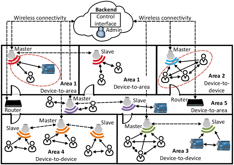
(a) DevLoc’s system combines Wi-Fi routers and light bulbs to enable device associations for mobile users and IoT boards.

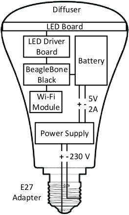
(b) DevLoc is based on the customized LocalVLC system [14] to realize visible light signaling for device grouping. We present the hardware platform of the deployed 3D-printed light bulb.

Figure 1: Enable seamless device associations using DevLoc

Fig. 1(a) presents the DevLoc framework for device grouping to combine radio-based communication like Wi-Fi covering larger areas and non radio-based communication such as light which is spatially more fine-grained due to walls, doors. We enrich existing lighting with visible light signaling for device grouping. Based on a master-slave principle of the light bulbs, we are able to semantically link multiple rooms or regions and thereby flexibly control the user’s spatial granularity. We use different colors in Fig. 1(a) to illustrate varying light patterns at the light bulbs for device associations. The dotted red circles highlight the association among different entities: a) device-to-device using only the device’s light signals or b) device-to-area using the device’s light signal and an area’s reference light signal for signal comparison. The goal of DevLoc is to ease data sharing among mobile user devices like tablets, smartphones, laptops, and static IoT boards. Inspired by [15, 16, 17] and as central part of DevLoc, our custom light bulb in Fig. 1(b) establishes a Wi-Fi link to the lighting configuration framework and broadcasts light patterns at a high frequency. On this basis, we can replace existing illumination units and hence we are able to restrict the problem of light pollution, where different visible lights would be overlapping for illumination and communication. We now describe in more detail the setup and working principle of DevLoc.

III-A Adaptable Spatial Granularity of Device Grouping

DevLoc allows to select proximity areas to define the geographic structure of the device associations. For example, Fig. 1(a) uses room numbers for area one and region names like corridor for area five. The lighting configuration framework runs at the backend and, initially, each light bulb and Wi-Fi router registers itself with the backend. As a result, DevLoc knows all light bulbs and their specific areas and randomly selects for each region one of the light bulbs as master light bulb, the remaining ones act as slaves. The backend randomly creates a light pattern for each registered master light bulb and the slave(s) broadcast the same light pattern with the master-slave mechanism for the light bulbs. We can dynamically choose the spatial granularity of device proximity by adapting the groups of light bulbs covering different regions. We can use the same light pattern over different rooms which are semantically the same region, e.g., area one in Fig. 1(a) to link two rooms. The size of rooms and regions like corridors, and the number and distribution of light bulbs define the achievable spatial granularity of device groupings. To achieve the most fine-granular user proximity, each light bulb works on its own as master. In our experiments, we identified the communication range of our custom light bulb of up to 10 m. Moreover, the master-slave mechanism of our light bulbs allows a minimum of technical adaptions on existing illumination. Only the master light bulbs need computing power to perform the device groupings, the slave light bulbs require only a radio connection, e.g., Wi-Fi or Bluetooth, to receive the commands from the corresponding master bulb.

III-B Triggering Device Grouping

We combine each master light bulb with a Wi-Fi router as a channel to the central configuration framework to maintain light patterns and for later device interaction. The light bulb continuously monitors the wireless connections of the Wi-Fi router and triggers device groupings. Due to the larger Wi-Fi coverage, one router can be combined with multiple master light bulbs. If there are no device groups yet and the Wi-Fi connections are changing, each linked master light bulb requests the continuously broadcasted light pattern received from the client(s). After receiving the client’s data, the master light bulb initiates the device grouping to infer which devices are in the same light communication range instead of being only in the same Wi-Fi coverage. In case of a new Wi-Fi client, the master light bulb runs the signal matching to infer the matching device group without affecting other devices. When a Wi-Fi device disappears at the router, the master light bulb deletes this single client from existing device groups.

Moreover, user mobility may also trigger device groupings. For static users who don’t move between rooms it is enough to observe the Wi-Fi connections for device grouping. In contrast, we need to manually start the device association via a predefined period, e.g., every few seconds, if users move between multiple regions but still connected to the same Wi-Fi router. To update the device grouping, we do not use signal strength changes of the user’s Wi-Fi connection because it can change unexpectedly and yields excessive false positives and false negatives causing frequent device grouping updates.

III-C Two Modes for Device Grouping: Device and Area

To support either location-based services (LBS) or proximity-based services (PBS), we are able to specify the mode of device groupings for each master light bulb: device-to-area grouping for LBS and device-to-device grouping for PBS. LBS needs to answer the question “where we are?” based on the absolute position of a user. In contrast, PBS needs to answer the question “who are we with?” based on context information to find co-location with other points of interest. We encounter three main differences between device-to-device and device-to-area groupings: 1) trigger point in time of the device association, 2) required number of user clients for device association, and 3) signal comparison between different entities which affect the resulting binding either device-to-device or device-to-area.

For device-to-device groupings we need at least two connected user clients at the Wi-Fi router to start the device grouping. To link a Wi-Fi client to a specific device group, the master light bulb randomly selects one client from each existing device group for signal matching. The participating user clients only know which other clients are nearby and not at which indoor region they are located. Thereby, we can only realize PBS like data sharing among close-by users and LBS are not feasible, e.g., sharing the menu of the cafeteria since the users are nearby to the canteen, because location-related information is missing using the device-to-device grouping.

For device-to-area groupings, after the user client connected to the Wi-Fi router the corresponding master light bulb(s) immediately start the device association and compare the client’s signal to the area’s reference signal. We achieve a direct binding between the device and area. Thereby, we know which device is in which area and at the same time which other devices are close-by. There is no limitation with respect to the number of connected user clients, e.g., at least two connected clients for device-to-device association. In general, device-to-device associations provide less location-specific information compared to device-to-area groupings.

III-D Generation and Recognition of Light Patterns

Our custom light bulb emits randomly generated light patterns for device associations. We independently create a random series of light on and off periods and combine them resulting in a light pattern. The duration of each light on and off period is in the range of [1, 5] ms. The minimum duration is constrained via the hardware of our light receiver, specifically, how fast the photodiode can be sampled. The maximum duration of each light on and off period is determined by avoiding unpleasant visual experience where light flickering effects are visible by human eyes. The light sender emits the light pattern in a loop for a restricted amount of time. To be able to differentiate light patterns, the length of the light pattern must be a multiple of two, i.e., after each light on period appears a light off period. To enhance the recognition rate of light patterns at the light receiver, we introduce a 10 % duration difference among light on and off series so that the time periods are sufficiently distinct. The photodiode at the light receiver samples the raw light signal as voltage in mV: a higher voltage refers to a light on period and a lower voltage refers to a light off period.

How to detect reoccurring patterns in the light signal? We use the cycle detection algorithm from [13] to find repeating patterns in our light signal. The algorithm supports signal matching of arbitrary co-aligned sensor data and reaches a reliable signal segmentation based on normalization. The algorithm’s input expects a vector of voltage amplitudes $z=(z_{1},...,z_{n})$ and the result is a sequence of consecutive light signal patterns. We use auto-correlation and distance calculation to find repeating signal parts. We can efficiently calculate the auto-correlation via the Wiener-Khinchin theorem [18] with complexity $n\cdot log(n)$

$$F_{R}(f) =FFT[z]$$

$$S(f) =F_{R}(f)\cdot F_{R}^{*}(f)\hskip 14.22636pt*\hat{=}\,\text{conjugate}$$

$$R(\tau) =IFFT[S(f)]$$

where $z$ are the voltage amplitudes. The auto-correlation $R(\tau)$ results in $m$ non-ambiguous local maxima $\zeta=\text{arg max}(R(\tau))=\{\zeta_{1},...,\zeta_{i}...,\zeta_{m}\}$. We compute the distances among all local maxima and a mean distance

$$\delta_{\text{mean}}=\left\lceil\frac{\sum_{i=1}^{m-1}\zeta_{i+1}-\zeta_{i}}{m-1}\right\rceil$$

at which $\delta_{\text{mean}}$ can be used to choose minima indices from $z$ representing signal patterns. To find the local minima $\mu$, every local maximum specifies a start point and $\delta_{\text{mean}}$ a search range

$$\mu =\{\mu_{1},...\mu_{i},...,\mu_{m-1}\}$$

$$\mu_{i} =\text{arg min}(z_{\zeta_{i}},z_{\zeta_{i}+1},...,z_{\zeta_{i}+\delta_{\text{mean}}})$$

Each $\mu_{j}$ refers to an index of a minimum in $z$ restricted to the range of $\delta_{\text{mean}}$. The indices in $\mu$ are used to separate the voltage amplitude $z$ into light cycles

$$Z =\{Z_{1},...,Z_{i},...,Z_{q}\}$$

$$Z_{i} =(z_{\mu_{\frac{i}{2}}},...,z_{\mu_{i}},...,z_{\mu_{\frac{i+1}{2}}-1})\text{ with }i=\{2,4,...,q\}$$

In our experiments, the rate of successfully extracted light patterns decreases significantly in case of sudden changes of light patterns caused by light interference. Therefore, we implement our own method to recognize light cycles considering the period of each light on and off phase. We define the light signal as a list of periods

$$\hat{z}=\{(s_{1},d_{1}),...,(s_{n},d_{n})\}$$

where $s_{n}\in\{0,1\}$ specifies if the light is on or off and $d_{i}\in\mathbb{Z}$ refers to the duration of each period. We combine similar signal parts with a difference smaller than 10 % because the light sender introduced a 10 % signal margin between the light on and off periods to improve the robustness of signal pattern detection. The remaining unique signal parts define the signal pattern including the period of each phase. To identify the light pattern, we overlay the light signal with a time window specified by the pattern length which is defined for the system.

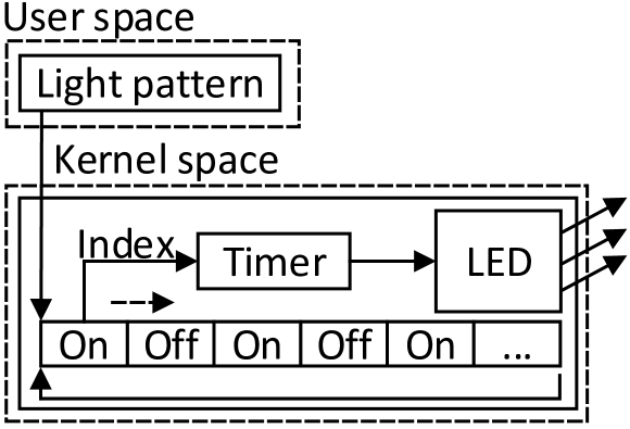
(a) Scheme of light sender

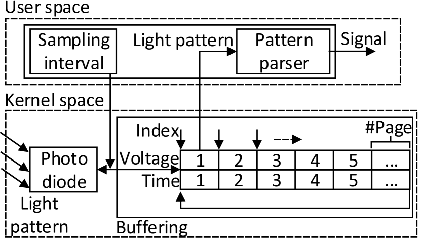
(b) Scheme of light receiver

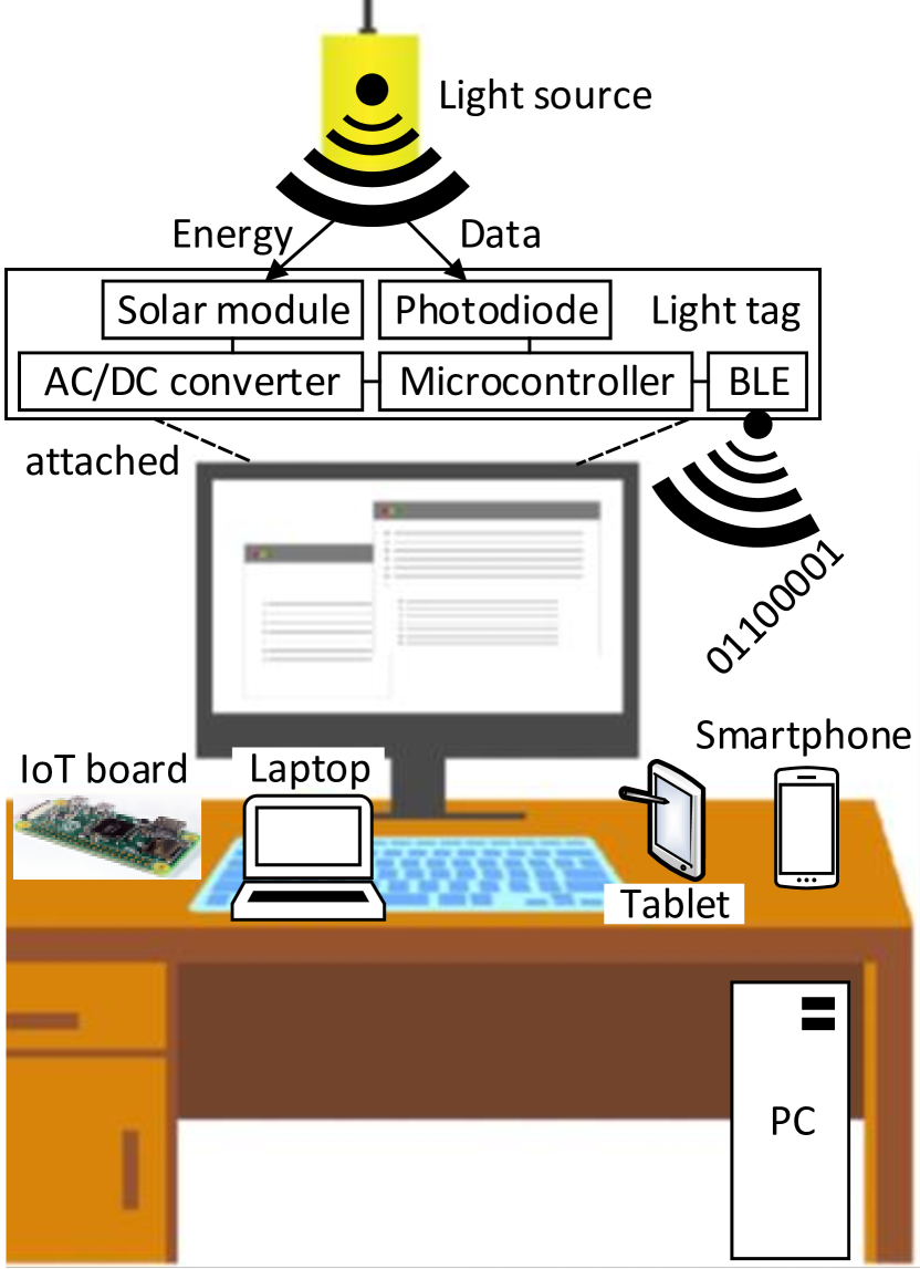
(c) Light tag for ubiquitous visible light signaling

Figure 3: Implementation details of VLC sender and receiver used by DevLoc. As future work we show the design of a light tag for improved end-device support of VLC.

III-E Technical Details of DevLoc

As system and development platform for our custom light bulb, we use the small, low-cost, single-board computer BeagleBone Black. We have implemented two Linux kernel modules to broadcast and receive light patterns. On the sender side, our custom light bulb broadcasts random light patterns via the light sender as shown in Fig. 3(a). The different light on and off periods of the signal pattern trigger two real-time kernel timers to switch the LED between on and off state. The custom light bulb consists of a power supply for the BeagleBone Black and during normal operation the battery is loaded and provides the power for the BeagleBone Black. The battery improves the service availability of DevLoc and maintains the lighting in case of a power blackout. In addition, the BeagleBone Black offers an API for visible light signaling and controls the LED transmitter and wireless modules such as Wi-Fi. On the receiving side, the light receiver in Fig. 3(b) samples the raw light signal via the photodiode. We have tested different sampling intervals, i.e., how often voltage values are sampled, and a sampling rate of 20 µs works reliably to detect light patterns. This affects the signal buffering to store and access light signals from the kernel module. We save voltages and the relative time chunked into pages and control the maximum page size and number of pages based on the sampling rate to provide sufficient information for signal parsing and available system’s memory.

We use MQTT for the communication among light bulbs. Via the subscription to the central backend, each master light bulb receives the configured light pattern which is then further published to the slave light bulb(s). Moreover, we use Python twisted as event-driven network programming framework to receive and send data between light bulbs and user clients. We establish a TLS network connection between the device grouping server and clients. The light bulb uses four different messages to query data for device grouping including raw light signal, detected light pattern, Wi-Fi, and Bluetooth scan data. The clients transmit the data in chunks of lines and the device grouping server buffers for each client the received raw data and merges them before the device association. The message format consists of a message type, a payload length, and the payload itself.

Regarding the VLC receiver, we aim to improve the end-device support for visible light signaling. Many user devices like personal computers do not have the required hardware such as a photodiode to sense light signals, while mobile user devices like smartphone and tablet provide a photodiode, e.g., for ambient light, but lack the ability to process light signals in real-time and require add-on hardware. For future work, we plan to shrink the light receiver to an appropriate (e.g., coin sized) volume for everyday usage towards ubiquitous visible light signaling. The foreseen light tag in Fig. 3(c) acts as proximate communication hub which can be easily attached to different end-user devices enabling light transmissions. The light source acts as energy source and at the same time as transmission medium. Thereby, the light tag works passively meaning it awakes for operation via energy induced by the solar module. During operation the light tag receives and processes light transmitted data in real-time and broadcasts it via Bluetooth Low Energy (BLE) to nearby end-user devices.

IV Evaluation of Device Associations via DevLoc

We evaluate the propagation characteristics of VLC to qualify the feasibility of real-world deployments of DevLoc. Besides that, we emulate two varying environments with static and moving users to highlight the performance of DevLoc in different environments. We identify, for each case, the best working device association with regard to high detection accuracy and fast runtime. Therefore, we perform a thorough parameter estimation of our device grouping including the sampling periods for light patterns, device localization for comparison, and training classifiers. Moreover, we select the best performing distance and correlation metrics and determine the most suitable time-series features for light patterns.

IV-A Propagation Characteristics of VLC

With regard to the use of DevLoc in the real world, we have evaluated the maximum attainable range of light patterns for two different LEDs as VLC transmitter in a dark room without interference from the surrounding light [14]. We used two LEDs: an omnidirectional LED with a weak light signal and a directional LED with a strong, beaming light signal. The directional LED reaches a maximum distance of 10 m, while the omnidirectional LED can cover a distance of 3 m. Furthermore, we identified via an experiment the FoV at the photodiode of the VLC receiver, the entire FoV ranges from 180° to 0°. The omnidirectional LED receives a range of 165°–50°, meaning opens at 165° and closes at 50°, and the directional LED achieves a FoV of 175°–5°. During our experiments, we have recognized that the impact of ambient light is decisive for VLC. Obviously, the directional LED is less sensitive to the ambient light compared to the omnidirectional LED. Nevertheless, with an active light source or direct sunlight acting as ambient light, the performance to detect signal patterns from the directional LED drops significantly. On the other hand, the omnidirectional LED only works reliably at a low ambient light intensity. For future work, we will adopt the algorithm in [19] which uses orthogonal codes to detect and isolate adjacent light sources. Thereby, we plan to enhance the robustness of DevLoc by supporting overlapping light patterns from different light bulbs.

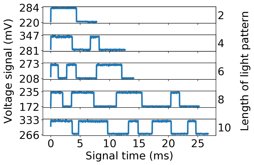
(a) Random light patterns

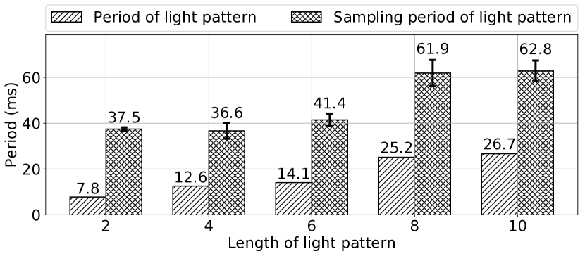
(b) Average sampling period

Figure 4: Sampling periods to detect light patterns with a varying length for device association

IV-B Parameter Estimation:
Sampling Periods of Light Patterns for Similarity Metrics

Our device grouping takes advantage of random light patterns in different spatial areas to establish device groups for data sharing. Which sampling periods are required to successfully detect light patterns? On the receiver side, we analyze the sampling time to be able to detect a valid light pattern within the time-series of voltage values. The light receiver is only able to recognize the light pattern when it starts repeating. We use five different light patterns for our evaluation with a varying length of light on and off periods as shown in Fig. 4(a). For each specific light pattern and over ten different test rounds, we choose a random start position within the light pattern and we extract a raw voltage signal via a monotonically increasing sampling time until all detected light patterns are valid. We classify a raw light signal as valid if all extracted light patterns have the same length $\in$ {2, 4, 6, 8, 10} and the duration of each light on and off phase is above 1 ms known by the generation of light patterns. Fig. 4(b) shows the necessary sampling periods to successfully recognize a reoccurring light pattern compared to the duration of a single light pattern. The sampling time is on average 3.1 times longer than the raw signal pattern. In our evaluation we use the identified sampling ranges for each length of signal pattern to randomly choose a raw voltage signal which is large enough for a reasonable signal comparison.

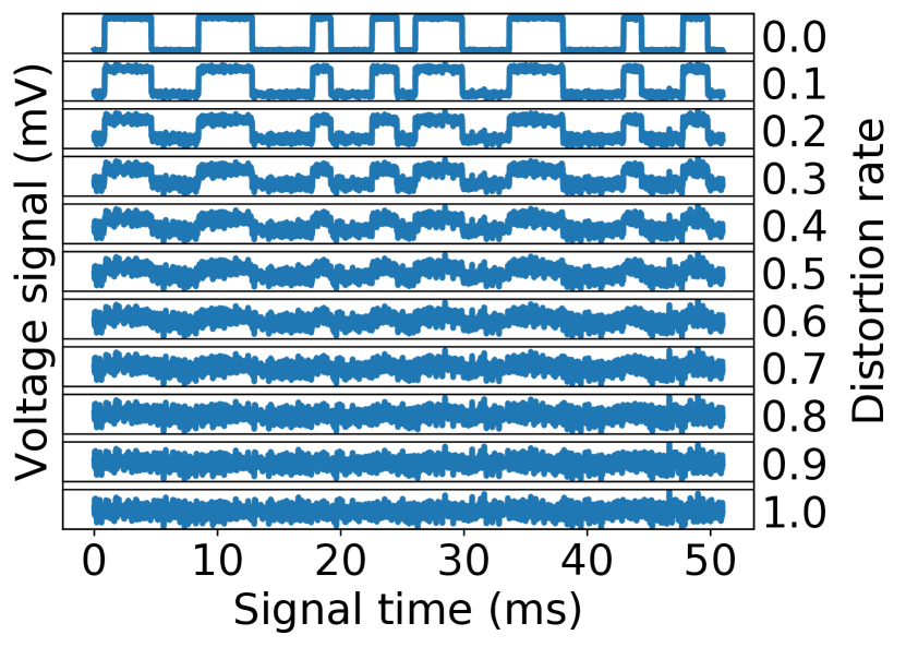
(a) Distorted light signals

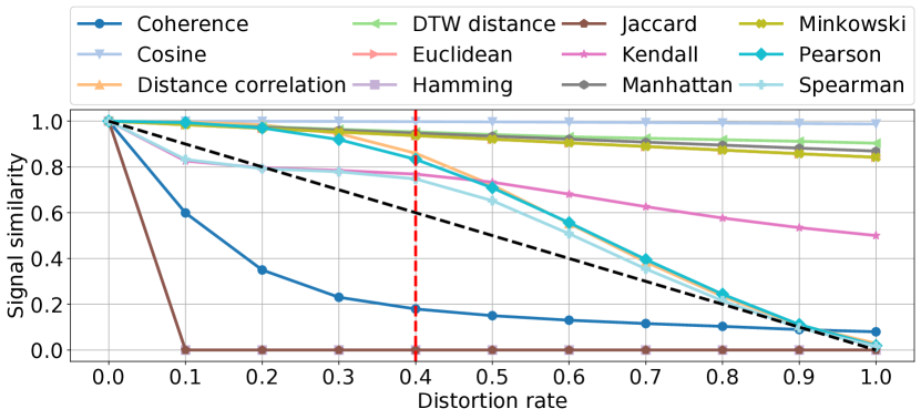
(b) Signal similarity of distorted signals

Figure 5: Analysis of signal similarity using distorted light signals for several distance and correlation metrics

TABLE I: Best working similarity and equalize methods for device association including similarity threshold and runtime

Similarity measure	Equalize method	Average metric	Similarity threshold	Runtime
Pearson	DTW	0.93	0.8	0.532 s
Spearman	DTW	0.89	0.9	0.532 s
DTW distance	DTW	0.89	0.7	0.506 s

IV-C Parameter Estimation:
Similarity Metrics for Light Patterns

We identify the best working similarity metrics for light patterns in terms of highest accuracy for group detection. We analyze the behavior of the similarity metrics by comparing raw light signals with the same increasingly distorted light signal such as in Fig. 5(a). Per similarity metric and signal distortion rate, the evaluation result in Fig. 5(b) shows the median similarity over ten rounds and each light pattern. The desired property of the similarity metric is that the similarity decreases in case of increasing dissimilarity between two time-series signals. Hence, we identify the following reasonable similarity metrics at a signal distortion rate of 40 %, highlighted as dotted red line in Fig. 5(b): Spearman with a similarity threshold of 0.74, Pearson with a similarity threshold of 0.83, and distance correlation with a similarity threshold of 0.86.

Besides that, we simulate a testbed with two clients for device grouping where we perform ten evaluation rounds for each combination among all light patterns $\in$ {2, 4, 6, 8, 10} to find the best working similarity metric and equalize method to unify signal lengths being able to compare them. In each run, we apply the similarity metrics mentioned in Fig. 5(b) and, as input, we randomly choose two light patterns and equalize their signal length using the methods $\in$ {fill, cut, dynamic time warping (DTW)}. Table I presents the three best working combinations of similarity metric, equalize method, and signal threshold in terms of highest average metric including accuracy, precision, recall, and F1-score weighted with 0.8 and lowest runtime weighted with 0.2. To calculate the result metrics, we assume that the two simulated clients are in the same region if the light signals have the same repeating pattern. We use these identified best working similarity measures to limit the runtime of our simulations for device grouping.

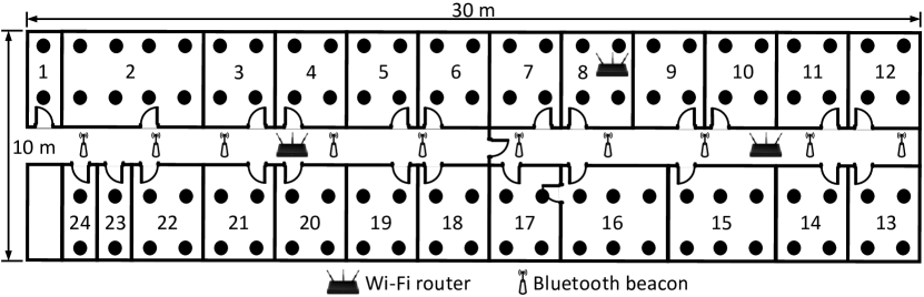
Figure 6: We model our university lab as simulation environment for device associations. For comparison with device localization, we take real traces of the Wi-Fi and Bluetooth environment at different positions.

IV-D Parameter Estimation:
Device Localization as Reference for Device Grouping

We use well-known device localization as reference to compare the results of our device grouping based on light patterns. We include a common indoor localization based on the similarity of Wi-Fi and Bluetooth signals [20]. Via an Android app we gather a list of Wi-Fi router and Bluetooth beacons containing MAC addresses and signal strengths (RSSI) for each measurement point ( ) at our university lab as shown in Fig. 6. We evaluate the sampling period, i.e., how many traces are required to achieve a reasonable localization accuracy. For a supervised machine learning approach with 10-fold cross validation, we have taken the following feature subset from the work in [21] to compare the list of Wi-Fi routers seen at two different measurement points, the same applies for the list of Bluetooth beacons:

• Number of overlapping devices

• Size of the union of the two lists

• Jaccard distance between the size of the intersection and the size of the union of the two lists

• Number of non-overlapping devices

• Manhattan distance of RSSI of overlapping devices

• Euclidean distance of RSSI of overlapping devices

• Spearman correlation of RSSI of overlapping devices

• Pearson correlation of RSSI of overlapping devices

• Share top device based on strongest RSSI

• Share at least one top device based on RSSI range $\pm$ 6 dB

We merge the different measurements for each room and perform binary classification among all rooms with multiple sampling periods $\in$ [2, 5, 10, 15, 20, 25, 30] s applying content-based filtering, support vector machine (SVM), and random forest. The content-based filtering uses the shortest cosine distance among room measurements to identify the user’s room. On average, the sampling period with 5 s achieves the highest accuracy for Wi-Fi and Bluetooth localization.

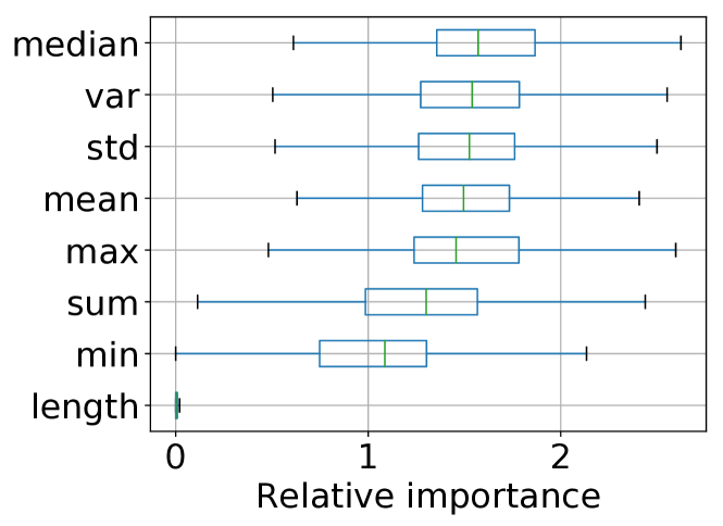
(a) Single light patterns for dynamic device-to-area simulation

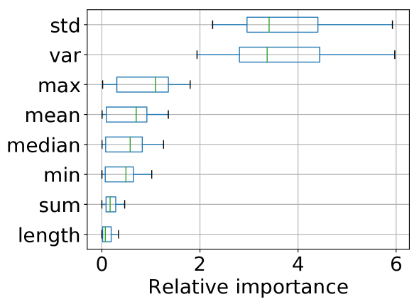
(b) Combination of light patterns for static device-to-device simulation

Figure 7: Selection of statistical features for light patterns via relative importance of trained machine learning models

IV-E Parameter Estimation:
Feature Selection for ML-based Device Grouping

Meaningful features are important for device grouping based on machine learning (ML) to achieve a good performance. Our feature selection identifies the features with highest entropy, i.e., information content, and lowest runtime. To find the most robust features in terms of distorted light patterns, we include light patterns with increasing white noise from 0 % to 100 %.

Raw light patterns for different simulations We use the combination of light patterns with different lengths for the static device-to-device simulation of our device grouping because it consists of only one room where we change the light pattern over time to keep the device groups up-to-date. Each master light bulb performs the proximity reasoning and is trained with a combination of light patterns with different lengths $\in$ {2, 4, 6, 8, 10}. In contrast, we use single light patterns for the dynamic device-to-area simulation of device grouping because it contains several rooms where the associated light pattern for each room remains the same over time. Each master light bulb is trained only for a specific, single light pattern with the same length.

Feature types We compute statistical features and time-series tailored features via tsfresh [22] for single and combination of light patterns. Tsfresh performs a time series feature extraction on basis of scalable hypothesis tests combining 63 time series characterization methods to identify the most meaningful features from a total of 794 time series features.

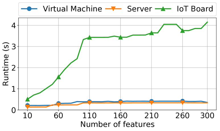
(a) Single light patterns for dynamic device-to-area simulation

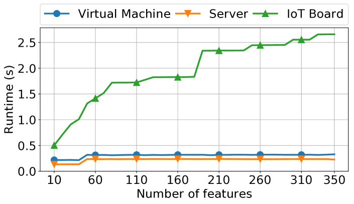
(b) Combination of light patterns for static device-to-device simulation

Figure 8: Runtime analysis of tsfresh features for light patterns to highlight the performance difference among test platforms

Best statistical features For feature selection of statistical features we take advantage of three different machine learning models: extra trees, gradient boosting, and random forest to identify the most important features. Fig. 7 shows the average relative importance of each statistical feature. In case of single light patterns, the relative importance is uniformly distributed over all features and only the feature length does not provide sufficient entropy. On the other hand, with the combination of light patterns, the variance and standard deviation outperforms all other features by 68 %.

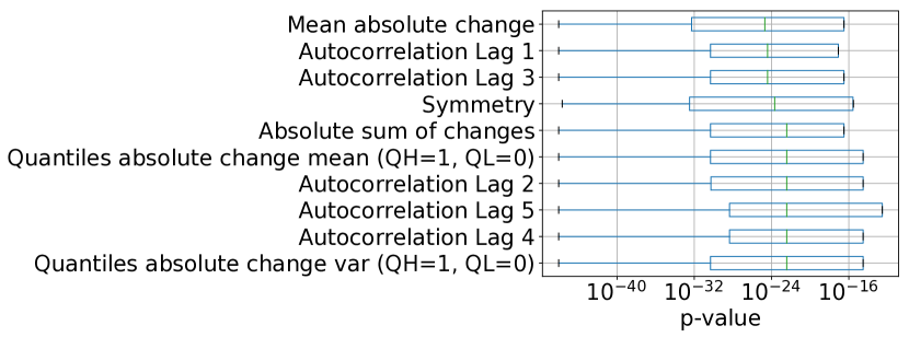
(a) Best ten features of single light patterns for dynamic device-to-area simulation

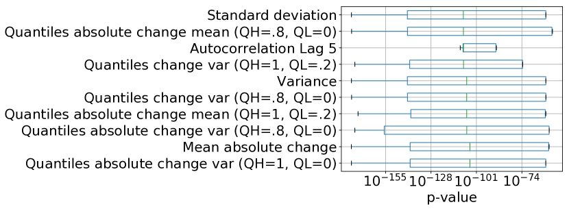
(b) Best ten features for combination of light patterns for static device-to-device simulation

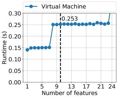
(c) Detailed runtime analysis of best time-series features at our simulation platform

Figure 9: Via tsfresh we select the ten most meaningful features of each light pattern type for device grouping. Moreover, we highlight the runtime to calculate these features at the virtual machine used as simulation platform for device grouping.

TABLE II: Testbed specifications for runtime analysis of feature selection used by device grouping

System	CPU	RAM
Server	40x Intel Xeon E5-2630 2.2 GHz	768 GB
Virtual machine (VM)	4x Intel Xeon E5-2630 2.2 GHz	32 GB
Next unit of computing PC (NUC)	4x Intel Core i5-6260U 1.8 GHz	16 GB
IoT board	1x ARM AM3358 1 GHz	0.5 GB

Runtime analysis of time-series features to select simulation platform We apply tsfresh for time-series feature selection to identify the most meaningful features of light patterns. Thereby, we highlight the runtime of feature calculation to evaluate the practicality of our proposed system where we aim to run the device associations directly at the light bulb which embeds an IoT board with limited hardware capabilities. Fig. 8 presents the feature runtime for single and combination of light patterns on three different test platforms described in Table VII. We sort the features according to their decreasing information content based on the hypothesis testing from tsfresh. For runtime comparison we calculate the relative runtime = $\nicefrac{{\text{runtime}}}{{\text{number of features}}}$ among the test platforms. In case of the single light patterns, tsfresh computes 300 features where the server achieves the fastest performance with a relative runtime of 2.63 ms per feature, the virtual machine is about 31 % slower with 3.46 ms per feature, and the IoT board is 6.2 times slower with 21.28 ms per feature. Using the combination of light patterns we achieve a similar runtime where tsfresh calculates 350 different time-series features. The server reaches a relative runtime of 2.11 ms per feature, the virtual machine with 3.17 ms, and the IoT board is by far the slowest platform with 14.99 ms per feature. Based on our findings from the feature runtime, we choose the virtual machine (VM) as simulation platform to evaluate DevLoc because the IoT board as desired platform is too slow when we repeat the device grouping at a higher rate. Note that this is just for the purpose of evaluation, the IoT board is still considered in other parts of the evaluation.

Best time-series features To improve the detection accuracy and limit the runtime of our device grouping, we select the ten most meaningful features of light patterns which are shown in Figs. 9(a) and 9(b). We use the p-value or probability value from tsfresh to select the most important features, the probability of finding the observed results when the null hypothesis is true. The lower the p-value the more significant is the feature. To ensure a reasonable performance for device grouping, Fig. 9(c) presents a detailed runtime analysis of features of light patterns computed at the virtual machine used as simulation platform for device grouping. It takes 253 ms to compute the ten most meaningful features for device associations which is fast enough to ensure the validity of our simulation results considering that we repeat device grouping every few seconds among multiple users.

IV-F Parameter Estimation: Sampling Period of Light Patterns to Train ML-based Device Grouping

We perform an offline evaluation of our device grouping to identify the best working sampling period for light patterns to train different classifiers. In our experiment, the device association ranges between two and ten grouping clients and we apply 10-fold cross validation for the classifiers: extra trees, gradient boosting, and random forest. These are trained via sampling periods $\in$ [30, 120] ms for different light patterns with signal length $\in$ {2, 4, 6, 8, 10} and selected tsfresh features from Fig. 9. We take the average results of our ML-based device grouping including accuracy, precision, recall, and F1-score. Fig. 10 shows that the sampling period of 50 ms achieves the best result with 0.91 over all classifiers compared to a sampling period of 120 ms with 0.74. The classifiers: extra trees, gradient boosting, and random forest achieve similar results.

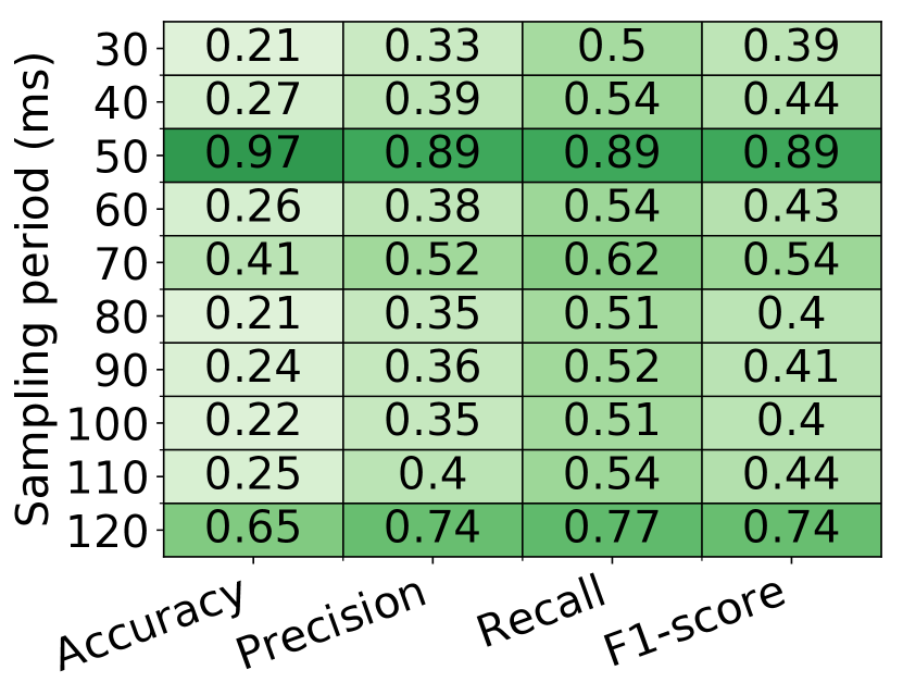
(a) Extra trees

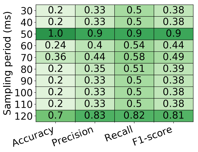
(b) Gradient boosting

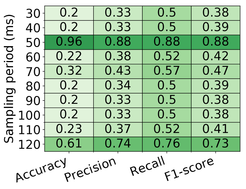
(c) Random forest

Figure 10: Parameter estimation of sampling period to train ML-based device association

IV-G Simulation Parameters for Device Grouping

To evaluate DevLoc, we run two different simulations with static and dynamic users based on a dedicated simulator. Table III shows the summarized best working parameters for device grouping (italicized). With persisted environmental data from our university lab as shown in Fig. 6, we perform a trace-driven simulation where each grouping client uses three different real traces: Wi-Fi and Bluetooth scans, and random light patterns with varying length. To achieve a realistic simulation, we emulate the network latency between the grouping server and the clients. Each client waits a random time within a predefined time range before sending the requested environment data to the grouping server. Thereby, we select a random start time within the sensing range for light patterns, Wi-Fi and Bluetooth scans. In addition, we randomly choose a sampling period within the identified best working sampling ranges.

TABLE III: Summarized settings from parameter estimation (highlighted in italic) and simulation parameters (highlighted in bold) for device grouping.

Simulation	Parameters
Static & Dynamic	Sampling period to train similarity classifiers	50 ms
	Similarity classifiers	Random forest, extra trees, gradient boosting
	Sampling period localization	5 s
	Localization classifiers	Content-based filtering, random forest, SVM
	Similarity equalize method	DTW
	Similarity threshold	0.7
	Similarity metrics	Pearson, Spearman
Dynamic	Rooms	[1, 2, 3, 4, 5, 6, 7, 8, 9, 10]
	Users	[3, 5, 10]
	Grouping frequency	[10, 20, 30] s
Static	Users	[2, 3, 4, 5, 6, 7, 8, 9, 10]
	Light patterns	[2, 4, 6, 8, 10]

TABLE IV: We identify best working classifiers and features for device grouping via simulations with static and moving users

Simulation	Grouping technique	Feature type	Result	Runtime	Accuracy	Precision	Recall	F1-score
Dynamic	Extra trees	Statistical	.83	0.26 s (1)	.75	1	.75	.83
	Content-based filtering	Wi-Fi	.84	0.61 s (7)	1	.78	.78	.78
	Content-based filtering	Bluetooth	.84	0.59 s (6)	.95	.81	.81	.81
	Gradient boosting	Selected statistical	.93	0.53 s (5)	.9	1	.9	.93
	Gradient boosting	Selected tsfresh	.93	1.58 s (8)	.9	1	.9	.93
	Pearson	Light signal	.95	0.28 s (2)	.95	.95	.95	.95
	Pearson	Light pattern	.95	0.47 s (4)	1	.93	.93	.93
	Pearson	Duration of light pattern	.95	0.46 s (3)	1	.93	.93	.93
Static	SVM	Wi-Fi	.31	2.61 s (6)	.32	.2	.44	.26
	Random forest	Bluetooth	.43	2.64 s (7)	.34	.48	.52	.38
	Pearson	Light signal	.64	2.06 s (5)	.25	.77	.79	.76
	Spearman	Duration of light pattern	.81	0.42 s (1)	1	.75	.75	.75
	Spearman	Light pattern	.81	0.49 s (3)	1	.75	.75	.75
	Gradient boosting	Statistical	.81	0.45 s (2)	1	.75	.75	.75
	Gradient boosting	Selected statistical	.83	0.75 s (4)	.89	.81	.81	.8
	Gradient boosting	Selected tsfresh	.96	4.02 s (8)	1	.94	.94	.94

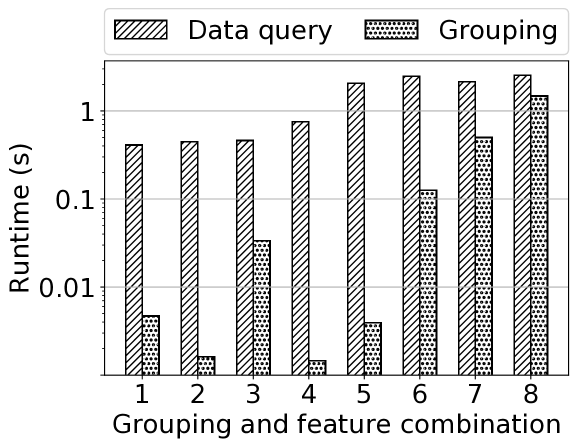
(a) Static device-to-device grouping

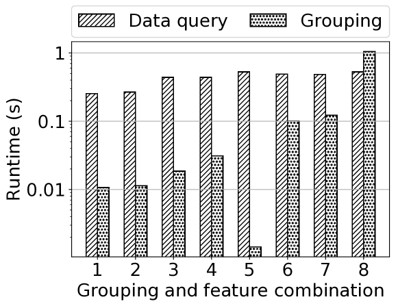
(b) Dynamic device-to-area grouping

Figure 11: Runtime analysis of different device groupings and signal features. To identify the grouping technique and feature type, the number of grouping and feature combination matches with the runtime order in Table IV mentioned in brackets.

IV-H Static Device-to-Device Simulation of Device Grouping

Simulation settings No user in the static simulation moves and every user stays in the same room. The grouping server immediately starts the device grouping when all devices are connected. The parameters for the static simulation are shown in Table III. We run the device grouping using random light patterns with different length $\in$ {2, 4, 6, 8, 10} and from at least two users up to ten users.

Simulation results Through 10-fold cross-validation, highlighted in bold in Table IV, we identify the best working device grouping technique in relation to a fast reasoning and a reasonable overall result, i.e., the average over accuracy, precision, recall, and F1-score. The device localization using Bluetooth and Wi-Fi features works worst whereas ML-based device grouping performs similar or slightly better than the signal similarity metrics such as Spearman and Pearson. Moreover, Fig. 11(a) presents the runtime of each method for device grouping sorted in ascending order. To perform device grouping, it takes around 1.41 s to receive data (83.93 % of total time) compared to the actual device grouping with 0.27 s (16.07 % of the total time).

For a thorough evaluation, we further analyze the performance of light patterns with different lengths for device grouping. The light pattern with four random on and off periods works best compared to a decrease of 9 % using the worst light pattern with ten random periods. The performance of light patterns with different lengths sorted by descending total result in brackets, i.e., average over accuracy, precision, recall, and F1-score: 4 (0.97), 2 (0.95), 6 (0.91), 8 (0.9), and 10 (0.88). Furthermore, we evaluate the performance using different number of grouping users. With six users we reach the highest total result of 0.97 because with less users the grouping signals miss crucial patterns and with more users the noise in the grouping signals grows which leads to a higher error rate for device associations. In detail, we show the number of grouping users with descending total result in brackets: 6 (0.97), 4 (0.94), 3 (0.93), 8 (0.93), 5 (0.92), 9 (0.92), 10 (0.92), 7 (0.92), and 2 (0.87).

IV-I Dynamic Device-to-Area Simulation of Device Grouping

Simulation settings In contrast to the static simulation, in the dynamic device-to-area simulation the users are moving between different rooms receiving varying light patterns. Our modeled simulation environment for device associations is shown in Fig. 6. The rooms are positioned in a rectangular arrangement with an inter room distance of 3 m and intra room distance of 2 m. We compute the distances among all room combinations. Using the duration of one simulation iteration of 20 min, we calculate a random path between the rooms for each user. Thereby, we distribute the random time as duration of stay over different rooms using a multinomial distribution. As a result, the user’s random path is a list of tuples with duration of stay and room, e.g., user A has the random path [(1, 120), (3, 300), …]. This means that the start position is in room 1 and after 120 s the user moves to room 3 and stays there for 5 min, and so forth. Hence, we randomly create user groups for each room at a specific time and for each movement between rooms every user chooses a random movement speed in the range of 1.25 to 1.53 m/s (4.5–5.5 km/h) [23]. If the users are in motion between two rooms they are in the corridor and not associated with any room. For device grouping, each room acts independently of other rooms and is linked with a unique location-dependent environment data containing Wi-Fi and Bluetooth scans, and light patterns. The overview of parameters for dynamic device-to-area simulation in Table III covers grouping frequency, number of users, and number of rooms.

Simulation results Table IV shows the best working device grouping (highlighted in bold) using 10-fold cross validation in terms of a fast runtime and a reasonable overall result, meaning the average over accuracy, precision, recall, and F1-score. Compared to the static device-to-device simulation, the device grouping based on similarity metrics works slightly better than ML-based device grouping. Further, the device localization using Wi-Fi and Bluetooth features reaches a similar result. The runtime of each method for device grouping is shown in Fig. 11(b) with ascending runtime from 0.26 s to 1.58 s. The median time is around 0.43 s (71.67 % of the total time) to receive data for device grouping whereas the device grouping itself lasts 0.17 s (28.33 % of the total time). Besides that, the frequency of device grouping with 20 s works best, the accuracy of device grouping decreases by 16 % with 30 s and with a 10 s frequency the accuracy decreases another 8 %. Furthermore, we analyze the performance of device grouping with a varying number of rooms, sorted after decreasing overall result in brackets: 1 (0.99), 2 (0.96), 3 (0.92), 5 (0.9), 6 (0.89), 4 (0.87), 8 (0.84), 7 (0.82), 9 (0.79), and 10 (0.76). The device grouping works best with less rooms because the more rooms the higher the risk that the user miss the up-to-date light pattern of the designated room due to movement between rooms.

Summarizing, Table IV presents two different best working classifiers and features for device grouping depending on the use case either with static or moving users. In both cases, we have an equal distribution between machine learning based and similarity based device grouping. Moreover, similar grouping techniques perform best, mainly the feature types are changing in varying conditions. Nevertheless, we favor the approach for device grouping in the scenario with multiple moving users because it is more realistic in practice.

V Practical Extension of DevLoc

DevLoc provides the basis to connect devices for data sharing among users. As a practical extension to enhance data privacy and ease the setup of data sharing, we analyze logs of device associations in terms of grouping patterns, e.g., time and frequency, to detect semantic device groups like personal and stranger’s devices. On this basis, we are able to create automated data sharing policies, such as sharing sensitive data only among personal devices.

V-A Artificial Log of Device Associations

In practice, DevLoc records device associations for further analysis to find semantic device groups. For evaluation we generate an artificial log of device associations to be able to analyze the device groups across different testbeds instead of using real-world data sets [24, 25] of social networks. To generate the log of device associations, we define a calendar for the simulation time including days $\in$ {all, holiday, weekend, workday} and time slots structuring the hours of the day: all $\in[0,24]$, night morning $\in[0,5]$, morning $\in[5,10]$, forenoon $\in[10,12]$, noon $\in[12,14]$, afternoon $\in[14,17]$, evening $\in[17,21]$, and evening night $\in[21,24]$. On this basis, we specify three different device groups $\in$ {personal, family & friends, well-known & stranger} with corresponding time encounter rules. For personal and family & friends devices: morning[workdays], evening[workdays], noon[all], afternoon[all], evening[all] in contrast to well-known & stranger devices where all encounter times are allowed: all[all], i.e., entirely random device encounters. We determine the possible device encounters based on the corresponding rule of the device group and then randomly distribute the device encounter time over the simulation duration, in our case one year (365 days). Finally, we clean the generated log by removing log entries with single and duplicated devices.

TABLE V: Best working classifiers and features to predict semantic device groups

Device group	Testbed	Classifier	Feature type	AUC	Cold start (days)	Accuracy	Precision	Recall	F1-score
Personal	Dense	Naive bayes	Contact frequency per week - sum	.99	23	.95	.92	.93	.92
	Medium	Extra trees	Grouping time per week - mean	.97	17	.93	.87	.92	.89
	Sparse	Ada boost	Contact frequency per week	.98	56	.96	.94	.93	.94
Family & Friends	Dense	Naive bayes	Contact frequency per week - sum	.99	17	.94	.92	.92	.92
	Medium	Gradient boosting	Grouping time per week - std	.85	72	.89	.84	.81	.83
	Sparse	Ada boost	Contact frequency per week	.98	55	.96	.94	.95	.95
Well-known & Stranger	Dense	Ada boost	Grouping time per week - sum	.98	16	.97	.97	.93	.95
	Medium	Ada boost	Contact frequency per week	.99	22	.97	.95	.95	.95
	Sparse	Ada Boost	Contact frequency per week	.99	45	.98	.97	.96	.96

V-B Semantic Log Analysis of Device Associations

Features for Log Analysis We create 43 different feature sets of three or ten dimensional features using the following information:

• how much time the devices are associated together per event, per day, and per week,

• how often the devices are associated together per day and per week, and

• the time ratio between association time and entire time frame per day and per week.

In addition, we calculate statistical measures like average and standard deviation of multiple combined features per event and per week. We use the statistical measures all together in a ten dimensional feature vector or we treat them individually as three dimensional feature vectors.

Testbeds for Log Analysis To simulate different test environments and compare the results, we introduce three environments with varying numbers of devices per device group and different grouping times, could be also more groups. The sparse environment includes three devices per device group and a grouping time in the range [10, 60] min, the medium environment has six devices per group and a grouping time of [20, 120] min, and the dense environment uses a grouping time of [30, 180] min and nine devices per device group.

Testbed: dense

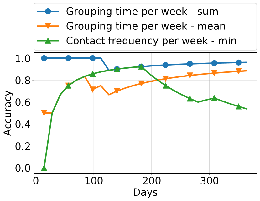
Testbed: medium

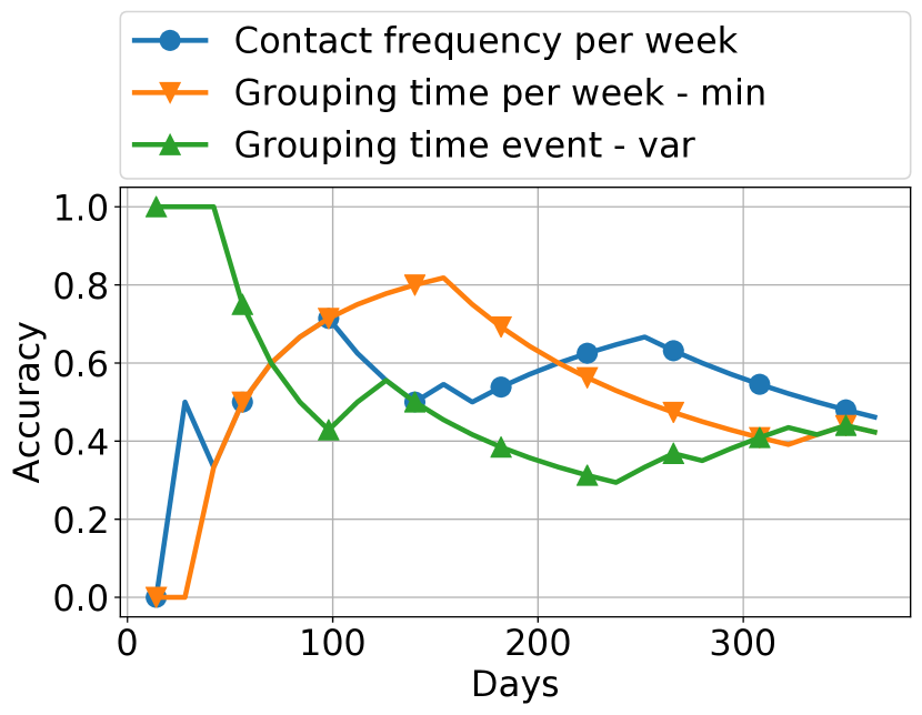
Testbed: sparse

(a) Detection accuracy of the three best performing features to cluster devices into three single device groups

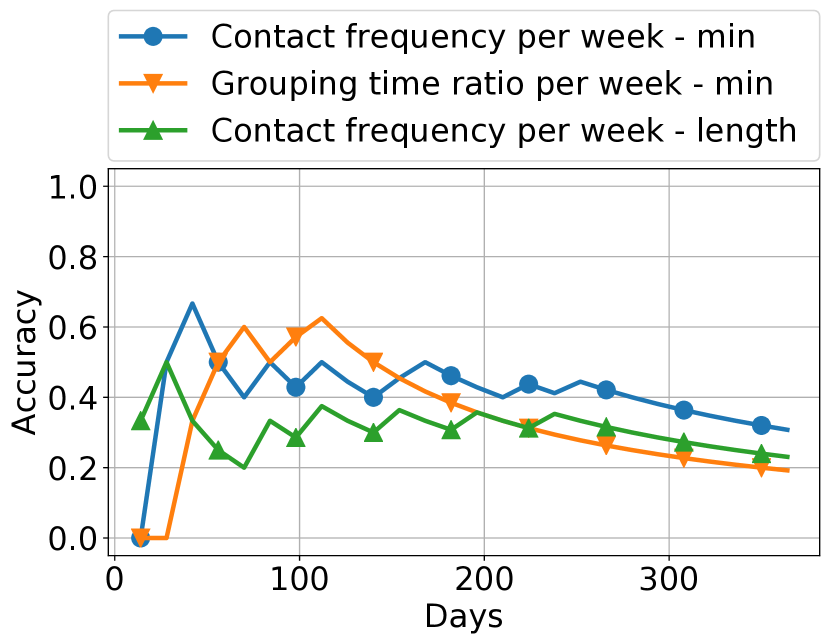
Testbed: dense

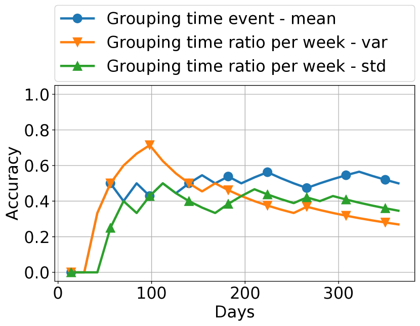
Testbed: medium

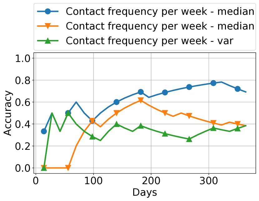
Testbed: sparse

(b) Detection accuracy of the three best performing features to cluster devices into seven mixtures of device groups

Figure 13: Detection granularity of different device groups over time: personal, family & friends, and well-known & stranger across testbeds with varying numbers of devices: dense, medium, and sparse.

Detection granularity of device groups over time Fig. 13 shows the clustering accuracy over time for each test environment with single or mixtures of device groups. We sort each cluster estimation after the mean accuracy in descending order and select the three best performing clustering methods. Our results show that in the dense and medium testbeds, we are able to reliably identify the three single device groups, in the sparse testbed the input data is not sufficient to estimate the device groups over time. The same holds true to detect the seven mixtures of device groups, over all testbeds it is impossible to reliably recognize the device groups. Our further analysis is restricted to three single device groups, if we can predict these device groups, we can also define data policies for a mixture of them.

In detail, at each time step $t$ we calculate the accuracy based on the estimated number of clusters via different clustering methods and the true number of clusters. Thereby, we highlight the temporal behavior to detect the number of device groups based on the log of device associations. Our log includes either three single device groups: personal, family & friends, well-known & stranger or seven mixtures of device groups, e.g., personal + family & friends. We use the following clustering methods to the range between 2 to 9 clusters:

• K-Means with elbow method using the total within sum of squares to measure the cluster compactness

• K-Means using silhouette score

• Hierarchical clustering using silhouette score

• Gaussian mixture using Bayesian Information Criterion

• Gaussian mixture using Akaike Information Criterion

• X-Means using K-Means++ for initial cluster centers

Find the best working features and classifiers to predict device groups Table V presents for each device class and testbed the best working classifier and feature type including the average area under the curve (AUC), cold start in days, accuracy, precision, recall, and F1-score. We model the problem to identify the best working classifiers and features to predict device groups as multi-class classification with the following device classes: 0 – personal, 1 – family & friends, and 2 – well-known & stranger. In total, we use 43 feature sets with a series of different classifiers via 10-fold cross validation. The classifiers include extra trees, gradient boosting, SVM, random forest, naive Bayes, and Ada boost. The cold start is the success criterion meaning after which time we are able to reliably predict the device class, the earlier the better. The cold start is defined by a threshold of 80 %, from this point in time (day), all result metrics including accuracy, precision, recall, and F1-score are above this threshold. Furthermore, we consider only prediction results with a cold start in the first quarter of the overall timeline of one year.

Stability to predict devices groups over time and across testbeds Table VI shows the most common combinations of classifier and feature per train and test environment among best performing prediction methods for semantic device groups. To be specific, we identify which combination of classifier and feature type works best over several test environments with varying numbers of devices and different device encounter times. Via 10-fold cross-validation, we train and test the classifier for each combination of {dense, medium, sparse} testbed and time of testing. Figs. 14(a) to 14(d) illustrate the average prediction result of the best performing classifiers and features, i.e., highest average detection accuracy over all device classes: personal, family & friends, and well-known & stranger to predict semantic device groups.

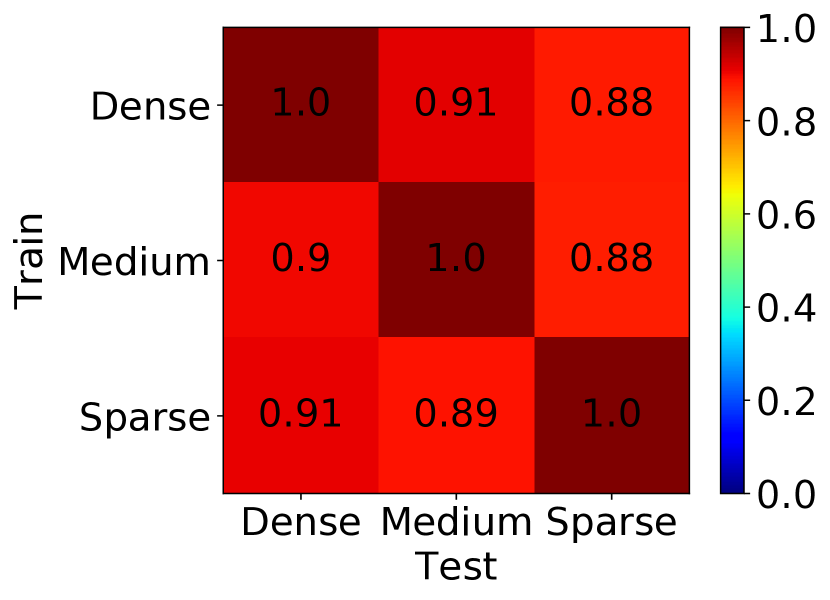
(a) Accuracy

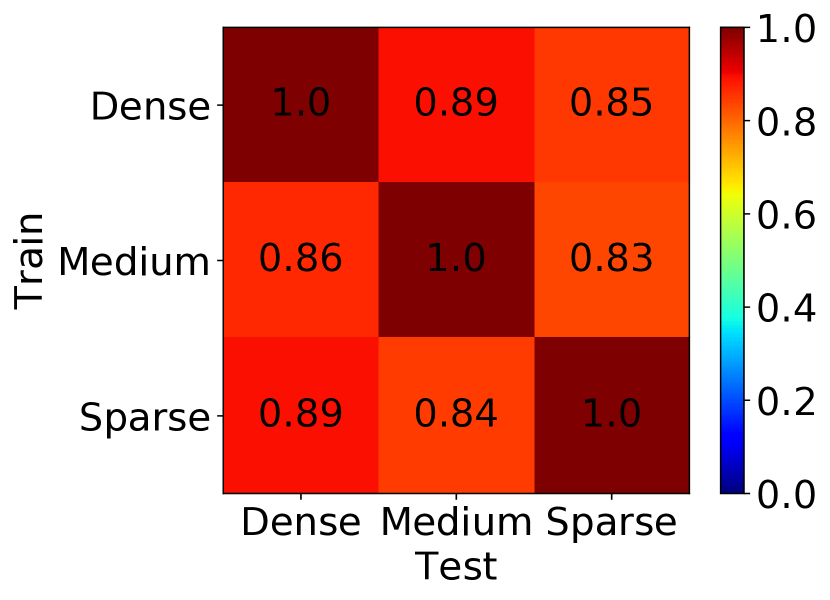
(b) Precision

(c) Recall

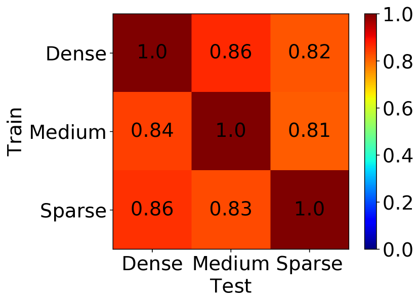
(d) F1-score

Figure 14: Average prediction result of the best performing classifiers and features to infer semantic device groups across testbeds with different number of devices

TABLE VI: Most common combination of classifier and feature among best prediction methods for semantic device groups

	Dense	Medium	Sparse
Dense	Ada Boost + Contact frequency per day	Naive Bayes + Grouping time ratio per week	Naive Bayes + Grouping time ratio per week
Medium	SVM + Grouping time per week - min	Ada Boost + Contact frequency per day	SVM + Grouping time per week - mean
Sparse	SVM + Grouping time per week	SVM + Grouping time per week	Ada Boost + Contact frequency per day

We encounter a potential privacy leakage by storing and analyzing device associations to infer semantic device groups. Countermeasures can be the anonymization of device activity logs, store the activity logs for a short period of time, and blockchain-secured device logging, or perform analysis in home only locally on the access point.

We conclude the evaluation of DevLoc to enable seamless device grouping based on visible light signaling. First, we analyze the characteristics of the VLC physical channel and afterwards we perform a thorough parameter estimation including pre-selection of distance and correlation measures for light patterns and feature selection for ML-based device association. On this basis, we run two device grouping simulations with a single room and static users and several rooms with moving users to find for each case the best working device grouping method. Besides that, we use the log of device associations to infer semantic device groups like personal, family or stranger’s devices to support data sharing policies, with whom sharing which data. For future extension, we plan to calculate a trust score [26] based on the log of device interactions from DevLoc to further enrich the semantic meaning of devices regarding allowed data sharing among devices.

VI Discussion

Due to the configuration framework of DevLoc based on visible light signaling integrated in surrounding lighting, we can support fine-granular device associations per room or region. In this way, we can realize our previously defined use cases for end users and IoT applications. By using the similarity of distance-limited light patterns, we are able to help Alice asking for the best way on the subway or Carol to record who is present at here meetings. Combined with LocalVLC [14], to incorporate our Morse-code inspired modulation scheme that can operate on off-the-shelf LEDs with low energy overhead, we are able to transmit data via light, e.g., location identifier, and not only light patterns. Thereby, we can support IoT applications, such as merging and filtering of location-tagged data from IoT boards and location-based access policies for consumer smart home platforms.

To enhance the user’s privacy for DevLoc, we will use private proximity testing at the light bulb during device grouping. Thereby, as part of the secure multi-party computation (SMC) problem, multiple parties are able to compute whether they are nearby without learning each other’s inputs. Homomorphic encryption [27] and garbled circuit [28] are two main techniques to solve the SMC problem, at which homomorphic encryption is more efficient compared to garbled circuit [29]. Usually homomorphic encryption is applied to a small amount of data, e.g., latitude and longitude, to compute the distance between two points of interest. In the appendix we analyze the runtime of fully homomorphic encryption for time-series data such as light patterns and we pinpoint the need of new cryptographic primitives for practical use.

Moreover, we plan to enhance DevLoc to be more resilient against adversaries performing relay attacks to trick our device grouping to include distant clients into the device group by relaying location-dependent light patterns from the intended space to remote clients. Besides that, we have to consider mitigation strategies against other attacks like spoofing the area’s light reference signal that clients use for association or periodically starting the device grouping every few seconds may introduce a frequent opportunity for potential attackers to identify themselves as part of the group.

VII Conclusion

DevLoc is a ready-to-use system solution that provides a seamless device grouping based on visible light signaling for data sharing. Our customized light bulb transmissions allows clients to detect cycles in the light patterns for device grouping. We perform a thorough evaluation of DevLoc via two different simulations with a single room and static users and multiple rooms with moving users. Thereby, we analyze the performance of several device grouping methods: signal similarity based on distance and correlation metrics, ML-based signal similarity, and as baseline the device localization using Wi-Fi and Bluetooth traces. Finally, we take advantage of the device grouping log to infer semantic device groups like personal, family or stranger’s devices to enhance the data privacy, with whom sharing which data.

Practicality of Fully Homomorphic Encryption for Private Proximity Testing To protect the user’s privacy during device grouping at the light bulb, we apply private proximity testing as an instance of the secure multi-party computation (SMC) problem where multiple parties compute whether they are nearby within a specific distance threshold without learning each other’s inputs. This protects the location data, e.g., light patterns, against a wide range of attacks, because it reveals no sensitive information to anyone. Homomorphic encryption [27] and garbled circuit [28] are two main techniques to solve the SMC problem, at which homomorphic encryption is more efficient compared to garbled circuit [29].

Our system model for proximity detection consists of a trusted party, a service provider, mobile users, and static IoT devices. The service provider is usually considered untrusted and should not learn the proximity test results. Our custom light bulb acts as trusted party and service provider, e.g., data sharing, among the nearby mobile devices. Usually homomorphic encryption is applied to a small amount of data to compute the distance between two points of interest, e.g., latitude and longitude of attractions like for LBS. In contrast, we analyze the runtime of fully homomorphic encryption for time-series data such as light patterns whether it is practically usable.

Testbeds To evaluate the performance of homomorphic encryption, we use the libraries: HElib [30] and SEAL [31] to compute the euclidean and cosine distance as similarity measure between two light patterns on three different platforms: server, NUC, and IoT board as described in Table VII.

TABLE VII: Testbed’s hardware specifications for runtime analysis of fully homomorphic encryption

System	CPU	RAM
Server	40x Intel Xeon E5-2630 2.2 GHz	768 GB
Virtual machine (VM)	4x Intel Xeon E5-2630 2.2 GHz	32 GB
Next unit of computing PC (NUC)	4x Intel Core i5-6260U 1.8 GHz	16 GB
IoT board	1x ARM AM3358 1 GHz	0.5 GB

Performance results Figs. 15(a) to 15(c) show the duration to initialize two different time-series each with a size in the range of [200, 21k] and compute the euclidean and cosine distance for proximity detection. We encounter data limits due to restricted system’s memory: on the IoT board the SEAL library achieves a maximum time-series length of 850 values compared to HElib with a size of 2k, and on the NUC only HElib reaches a data limit of 20k values. We analyze the library performance per test platform over all operations $\in$ {initialization, euclidean, cosine} and time-series values. The HElib library works fastest at the server, the NUC is about 33 % slower, and IoT board is 11.7 times slower compared to the NUC. In comparison, the SEAL library performs best at the server, the NUC is 19 % slower, and the IoT board takes 51 times longer.

We compute the runtime per operation over all test platforms and time-series values. The initialization of time-series vectors takes on average 0.43 s using SEAL and 9 s with HElib, hence HElib is around 11.67 times slower per vector element. For the euclidean distance, the HElib library requires between [36, 569] s and the SEAL library achieves [56, 397] s, the relative runtime per vector element of HElib with 0.11 s is 2.16 times faster compared to SEAL (0.24 s). For the cosine distance, the HElib library takes on average between [135, 2137] s and using the SEAL library lasts [166, 1187] s, the relative runtime per vector element of HElib with 0.42 s is 1.72 times faster compared to SEAL with 0.72 s.

We compare the runtime performance of the baseline using two-dimensional positions like for LBS with our generated light patterns ranging between 1762 to 3717 raw voltage signals. We compute the average runtime for each homomorphic encryption library over all test platforms and operations at which the light pattern contains on average 1417 voltage values. The HELib library is slower with a runtime of 0.72 s for the baseline and the light pattern takes around 63.39 s, with a normalized delta of 90.99 % over the time-series length. The faster SEAL library achieves a runtime of 0.09 s for the baseline and 31.8 s for the larger light signal which results in a normalized delta of 63.34 %.

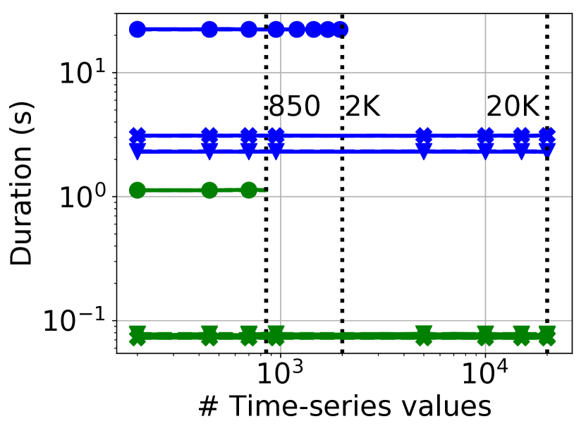
(a) Initialization

(b) Euclidean distance

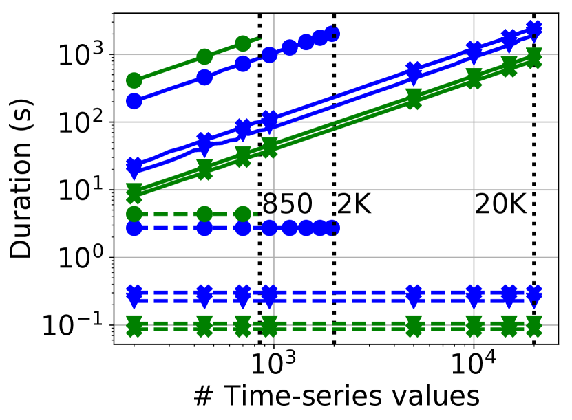
(c) Cosine distance

Figure 15: Performance of fully homomorphic encryption over three different testbeds: server, NUC, and IoT board using two libraries: HElib and SEAL. The baseline refers to the distance calculation using only two-dimensional positions compared to time-series with hundreds of values.

In a nutshell, our aim is to enhance user’s privacy by applying homomorphic encryption to secure the time-series data processing of our device grouping. The runtime analysis motivates the need of new cryptographic primitives for efficient time-series data analysis. The up-to-date homomorphic encryption is too slow to be usable in practice with a runtime of about 30 s per distance computation whereas we require a maximum runtime of 0.5 s per calculation.

References

- [1] A. Narayanan, N. Thiagarajan, and M. Lakhani, “Location Privacy via Private Proximity Testing,” in Proceedings of the 18th Annual Network and Distributed System Security Symposium (NDSS), 2011.
- [2] S. Mare, L. Girvin, F. Roesner, and T. Kohno, “Consumer Smart Homes: Where We Are and Where We Need to Go,” in Proceedings of the 20th International Workshop on Mobile Computing Systems and Applications (HotMobile), 2019, pp. 117–122.
- [3] M. K. Chong and H. W. Gellersen, “How Groups of Users Associate Wireless Devices,” in Proceedings of the SIGCHI Conference on Human Factors in Computing Systems (CHI), 2013, pp. 1559–1568.
- [4] M. K. Chong, R. Mayrhofer, and H. Gellersen, “A Survey of User Interaction for Spontaneous Device Association,” ACM Computing Surveys, vol. 47, no. 1, pp. 1–40, 2014.
- [5] Y.-S. Kuo, P. Pannuto, K.-J. Hsiao, and P. Dutta, “Luxapose: Indoor Positioning with Mobile Phones and Visible Light,” in Proceedings of the 20th International Conference on Mobile Computing and Networking (MobiCom), 2014, pp. 447–458.
- [6] Z. Yang, Z. Wang, J. Zhang, C. Huang, and Q. Zhang, “Lightweight Visible Light Positioning for Wearables,” GetMobile: Mobile Computing and Communications, vol. 19, no. 3, pp. 18–21, 2015.
- [7] ——, “Wearables Can Afford: Light-Weight Indoor Positioning with Visible Light,” in Proceedings of the 13th Annual International Conference on Mobile Systems, Applications, and Services (MobiSys), 2015, pp. 317–330.
- [8] D. Schürmann and S. Sigg, “Secure Communication Based on Ambient Audio,” Secure Communication Based on Ambient Audio, vol. 12, no. 2, pp. 358–370, 2013.
- [9] M. Miettinen, N. Asokan, T. D. Nguyen, A.-R. Sadeghi, and M. Sobhani, “Context-Based Zero-Interaction Pairing and Key Evolution for Advanced Personal Devices,” in Proceedings of the ACM SIGSAC Conference on Computer and Communications Security (CCS), 2014, pp. 880–891.
- [10] R. Mayrhofer and H. Gellersen, “Shake Well Before Use: Intuitive and Secure Pairing of Mobile Devices,” IEEE Transactions on Mobile Computing, vol. 8, no. 6, pp. 792–806, 2009.
- [11] A. Varshavsky, A. Scannell, A. LaMarca, and E. de Lara, “Amigo: Proximity-Based Authentication of Mobile Devices,” in Proceedings of the 9th International Conference on Ubiquitous Computing (UbiComp), 2007, pp. 253–270.
- [12] R. Jin, L. Shi, K. Zeng, A. Pande, and P. Mohapatra, “MagPairing: Pairing Smartphones in Close Proximity Using Magnetometers,” IEEE Transactions on Information Forensics and Security, vol. 11, no. 6, pp. 1306–1320, 2016.
- [13] D. Schürmann, A. Brüsch, N. Nguyen, S. Sigg, and L. Wolf, “Moves like Jagger: Exploiting variations in instantaneous gait for spontaneous device pairing,” Pervasive and Mobile Computing, vol. 47, pp. 1–12, 2018.
- [14] M. Haus, A. Y. Ding, and J. Ott, “LocalVLC: Augmenting Smart IoT Services with Practical Visible Light Communication,” in Proceedings of the 20th IEEE International Symposium on “A World of Wireless, Mobile and Multimedia Networks” (WoWMoM), 2019, pp. 1–9.
- [15] S. Schmid, J. Ziegler, G. Corbellini, T. R. Gross, and S. Mangold, “Using Consumer LED Light Bulbs for Low-Cost Visible Light Communication Systems,” in Proceedings of the 1st ACM MobiCom Workshop on Visible Light Communication Systems (VLCS), 2014, pp. 9–14.
- [16] Gummeson, Jeremy, J. McCann, C. Yang, D. Ranasinghe, S. Hudson, and A. Sample, “RFID Light Bulb: Enabling Ubiquitous Deployment of Interactive RFID Systems,” Proceedings of the ACM on Interactive, Mobile, Wearable and Ubiquitous Technologies (IMWUT), vol. 1, no. 2, 2017.
- [17] S. Schmid, T. Bourchas, S. Mangold, and T. R. Gross, “Linux Light Bulbs: Enabling Internet Protocol Connectivity for Light Bulb Networks,” in Proceedings of the 2nd International Workshop on Visible Light Communications Systems (VLCS), 2015, pp. 3–8.
- [18] L. Cohen, “Generalization of the Wiener-Khinchin Theorem,” IEEE Signal Processing Letters, vol. 5, no. 11, pp. 292–294, 1998.
- [19] A. U. Guler, T. Braud, and P. Hui, “Spatial Interference Detection for Mobile Visible Light Communication,” in Proceedings of the IEEE International Conference on Pervasive Computing and Communications (PerCom), 2018, pp. 1–10.
- [20] H. S. Maghdid, I. A. Lami, K. Z. Ghafoor, and J. Lloret, “Seamless Outdoors-Indoors Localization Solutions on Smartphones,” ACM Computing Surveys, vol. 48, no. 4, pp. 1–34, 2016.
- [21] P. Sapiezynski, A. Stopczynski, D. Kofoed Wind, J. Leskovec, and S. Lehmann, “Inferring Person-to-person Proximity Using WiFi Signals,” Proceedings of the ACM on Interactive, Mobile, Wearable and Ubiquitous Technologies, vol. 1, no. 2, pp. 1–20, 2017.
- [22] M. Christ, N. Braun, J. Neuffer, and A. W. Kempa-Liehr, “Time Series FeatuRe Extraction on basis of Scalable Hypothesis tests (tsfresh – A Python package),” Neurocomputing, vol. 307, pp. 72–77, 2018.
- [23] N. Carey, “Establishing Pedestrian Walking Speeds,” Portland State University, 2005.
- [24] S. Firdose, L. Lopes, W. Moreira, R. Sofia, and P. Mendes, “CRAWDAD dataset copelabs/usense (v. 2017-01-27),” Downloaded from https://crawdad.org/copelabs/usense/20170127, Jan. 2017.
- [25] R. I. Ciobanu and C. Dobre, “CRAWDAD dataset upb/hyccups (v. 2016-10-17),” Downloaded from https://crawdad.org/upb/hyccups/20161017, Oct. 2016.
- [26] D. Chatzopoulos, M. Ahmadi, S. Kosta, and P. Hui, “OPENRP: A Reputation Middleware for Opportunistic Crowd Computing,” IEEE Communications Magazine, vol. 54, no. 7, pp. 115–121, 2016.
- [27] C. Gentry, “Fully Homomorphic Encryption using Ideal Lattices,” in Proceedings of the 41st Annual ACM Symposium on Theory of Computing (STOC), M. Mitzenmacher, Ed., 2009, pp. 169–178.
- [28] A. C. Yao, “Protocols for secure computations,” in Proceedings of the 23rd Annual Symposium on Foundations of Computer Science (SFCS), 1982, pp. 160–164.
- [29] P. Hallgren, M. Ochoa, and A. Sabelfeld, “InnerCircle: A Parallelizable Decentralized Privacy-Preserving Location Proximity Protocol,” in Proceedings of the 13th Annual Conference on Privacy, Security and Trust (PST), 2015, pp. 1–6.
- [30] “IBM,” https://github.com/homenc/HElib, 2019.
- [31] “Microsoft SEAL (release 3.2),” https://github.com/Microsoft/SEAL, 2019.