Slow magnetosonic wave absorption by pressure induced ionization-recombination dissipation

Abstract

A new mechanisms for damping of slow magnetosonic waves (SMW) by pressure induced oscillations of the ionization degree is proposed. An explicit formula for the damping rate is quantitatively derived. Physical conditions where the new mechanism will dominate are briefly discussed. The ionization-recombination damping is frequency independent and has no hydrodynamic interpretation. Roughly speaking large area of partially ionized plasma are damper for basses of SMW while usual MHD mechanisms operate as a low pass filter. The derived damping rate is proportional to the square of the sine between the constant magnetic field and the wave-vector. Angular distribution of the spectral density of SMW and Alfvén waves (AW) created by turbulent regions and passing through large regions of partially ionized plasma is qualitatively considered. The calculated damping rate is expressed by the electron impact cross section of the Hydrogen atom and in short all details of the proposed damping mechanisms are well studied.

I Short Introduction

Behind purely fundamental interest for plasma physics propagation of hydromagnetic (nowadays known as magnetohydrodynamic ) waves attracted significant attention and was strongly simulated by the development of the physics of solar atmosphere and the eternal problems related to its heating.Alfven:42 ; Alfven:47 ; LL8 It has already been confirmed that the magnetohydrodynamic (MHD) waves (both incompressible and compressible) are present in the solar atmosphere and they have already been considered for heating of the solar chromosphere and corona.Mond:94 ; Campos:99 ; Wijn:07 ; Ruderman:12 Models adapted to study heating problems of solar atmosphere include two fluids coupled through collisions and chemical reactions, such as impact ionization and radiative recombination with imposed initial thermal and chemical equilibrium. Within this approach the plasma heating is dominantly wave-based and the main energy source for heating are the excited fast magnetosonic fluctuations,Maneva:17 while older studies of FMW heating can be found in Ref. Zhelyazkov:87, for instance.

It is worthwhile to mention also works on overreflection or swing amplification in shear flow of slow magnetosonic waves (SMW); see for example Refs. Hristov:11, ; Gogoberidze:04, .

In a review on partially ionized astrophysical plasmasBallester:18 it is shown that viscosity plays no important role in the damping of chromospheric Alfvén waves and recently it is concluded that the solar corona electrical resistivity has only very small impact, while and thermal conduction and viscosity contribute equally.Perelomova:20 Therefore, the question of chromospheric heating due to the ion-neutral interaction will require further studies in the future. A complete review on the problem requires many hundred citations, but here we mention the importance of two fluid approach for consideration of MHD waves in partially ionized plasmas.Zaqarashvili:11

I.1 Scenario

When a slow magnetosonic wave (SMW) propagates through partially ionized plasma, the oscillations of the pressure creates oscillations of the temperature and generates small oscillations of the degree of ionization $\alpha$. Those pressure induced deviations of the chemical equilibrium gives an extra entropy production and energy dissipation of the SMW.

This additional mechanism does not work for the Alfvén waves (AW) and in spite of common dispersion and damping of AW and SMW in (MHD) approach at small magnetics field their ionization-recombination absorption can be completely different.

The purpose of the present work is to present an explicit formula for the chemical damping and to consider in short when the predicted new damping mechanism is important and dominates and how it can be observed.

The article is organized as follows. In order to create the necessary system of notions and notations following Landau and LifshitzLL8 in the next Sec. II we will recall the physics of SMW. Then we derive in Sec. III our new result for ionization-recombination absorption. Finally we will discus in Sec. IV

II Recalling SMW

In this section we will repeat these details which are common for Alfvén waves (AW) and SMW. The differences between AW and SMW which are our new result we derive after that.

II.1 Dispersion of MHD Waves

Low density hydrogen plasma we approximate as a cocktail of ideal gases of electrons, protons and neutral atoms with pressure $p$ and mass density $\rho$

$$p=nT,\qquad n=n_{e}+n_{p}+n_{0},$$ (1)

$$\rho=n_{\rho}M,\qquad n_{\rho}=n_{p}+n_{0},$$ (2)

where temperature $T$ is written in energy units and $M$ is the proton mass. The sound velocity is defined by the adiabatic compressibility

$$c_{s}=\sqrt{\left(\frac{\partial p}{\partial\rho}\right)_{\!\!s}},$$ (3)

for which the standard expression from the averaged atomic mass of the cocktail $\left<M\right>$

$$c_{s}=\sqrt{\frac{\gamma_{p}T}{\left<M\right>}},\quad\left<M\right>=\frac{n_{p}M+n_{0}M+n_{e}m}{n_{p}+n_{0}+n_{e}},$$ (4)

$$c_{v}=3/2,\quad c_{p}=c_{v}+1=5/2,\quad\gamma=c_{p}/c_{v}=5/3$$ (5)

where $c_{v}$ and $c_{p}$ are the heat capacities per atom and $m$ is the electron mass.

Small amplitude MHD waves we treat as small variations of the magnetic field $\mathbf{b}$, density $\rho^{\prime}$, pressure $p^{\prime}$ and temperature $T^{\prime}$

$$\mathbf{B}=\mathbf{B}_{0}+\mathbf{b},\quad\rho=\rho_{0}+\rho^{\prime},$$ (6)

$$p=p_{0}+p^{\prime},\quad T=T_{0}+T^{\prime}$$ (7)

from their constant values. The index $0$ we omit where it is obvious. The variations of the pressure are related with variations of the density

$$p^{\prime}\approx c_{s}^{2}\rho^{\prime},\quad$$ (8)

according the definition of the sound speed. Here we recall also the equations of state $pV^{\gamma}=\mathrm{const}$ and $TV^{1/c_{v}}=\mathrm{const}$ for $S=\mathrm{const}$ (constant entropy $S$) and give the relations between variations of the temperature, pressure and densityLL5

$$\frac{T^{\prime}}{T}=\frac{1}{c_{v}}\frac{\rho^{\prime}}{\rho}=\frac{1}{c_{p}}\frac{p^{\prime}}{p},\quad\frac{\rho^{\prime}}{\rho}=\frac{1}{\gamma}\frac{p^{\prime}}{p},\quad\gamma\equiv\frac{c_{p}}{c_{v}}=\frac{5}{3}.$$ (9)

For a weak amplitude plane wave the variations of all variables are proportional to the imaginary exponent $\propto\mathrm{e}^{\mathrm{i}(\mathbf{k}\cdot\mathbf{r}-\omega t)}$ and phase velocity $u\equiv\omega/k$ the ratio between the frequency $\omega$ and the modulus $k=|\mathbf{k}|$ of the wave-vector. For a plane wave the time $t$ and space $\mathbf{r}$ derivatives are reduced to multiplication

$$\partial_{t}=-\mathrm{i}\omega,\qquad\nabla=\mathrm{i}\mathbf{k}$$ (10)

and the MHD equations, omitting index $0$ and imaginary unit $\mathrm{i}$, readsLL8

$$-\omega\rho\mathbf{v}=-c_{s}^{2}\mathbf{k}\rho^{\prime}+\mathbf{B}\times\left(\mathbf{k}\times\mathbf{b}\right)/\mu_{0},\quad\mu_{0}=4\pi,$$ (11)

$$-\omega\mathbf{b}=\mathbf{k}\times\left(\mathbf{v}\times\mathbf{B}\right),\quad\omega\rho^{\prime}=\rho\mathbf{k}\cdot\mathbf{v},\;\;\varepsilon_{0}=1/4\pi,$$ (12)

where $\mathbf{k}\cdot\mathbf{b}=0$. We use Gaussian units but in SI&C: $\mu_{0}\,*=10^{-7}$ and $\varepsilon_{0}/=c^{2}\,10^{-7}$, i.e. all formulae in the present work are written in system invariant form. In Heaviside–Lorentz units $\mu_{0}=1$ and $\varepsilon_{0}=1$. The $x$-axis is chosen along the wave-vector $\mathbf{k}=k\mathbf{e}_{x}$, and $y$-axis is in the plane of the wave-vector and the constant magnetic field

$$\mathbf{B}=B_{x}\mathbf{e}_{x}+B_{y}\mathbf{e}_{y},\quad B_{x}=B\cos\theta,\quad B_{y}=B\sin\theta,$$

see Fig. 1.

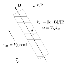
Figure 1: Geometry of propagating of SMW in a constant external magnetic field $\mathbf{B}$. The group velocity of the propagating wave packet $\mathbf{v}_{\mathrm{gr}}$ is along the external magnetic field. The wave vector $\mathbf{k}$ is along the normal of wave fronts (equiphase planes) shown here with lines parallel to the $y$ axis.

The unit vector along the external magnetic field is

$$\mathbf{e}_{B}=\mathbf{B}/B=\cos\theta\,\mathbf{e}_{x}+\sin\theta\,\mathbf{e}_{y}$$ (13)

Dividing by $k$, the nonzero components of the MHD equations Eqs. 11 and 12 read

$$\rho u\left(1-\frac{c_{s}^{2}}{u^{2}}\right)\!v_{x}=B_{y}b_{y}/\mu_{0},\quad$$ (14)

$$\rho uv_{y}=-B_{x}b_{y}/\mu_{0},$$ (15)

$$ub_{y}=B_{y}v_{x}-B_{x}v_{y}.$$ (16)

Expressing velocity components $v_{x}$ and $v_{y}$ from the first two equations and substituting it in the third one gives a quadratic equation for the phase velocity $u=\omega/k$ which have the solutions describing fast (f) and slow (s) magnetosonic wavesLL8

$$u^{2}_{\mathrm{f,s}}=\frac{1}{2}\left\{V_{\mathrm{A}}^{2}+c_{s}^{2}\pm\left[(V_{\mathrm{A}}^{2}+c_{s}^{2})^{2}-4c_{\theta}^{2}V_{\mathrm{A}}^{2}c_{s}^{2}\right]^{1/2}\right\}.$$ (17)

For small magnetic fields for SMW wave we have

$$u=u_{s}\approx V_{\mathrm{A}}c_{\theta}\ll c_{s},\qquad c_{\theta}\equiv|\cos\theta|,$$ (18)

where

$$\mathbf{V}_{\mathrm{A}}\equiv\frac{\mathbf{B}}{\sqrt{\mu_{0}\rho}},\quad\rho V_{\mathrm{A}}^{2}=B^{2}/\mu_{0}$$ (19)

is the speed of AW and $u_{\mathrm{A}}\equiv V_{\mathrm{A}}c_{\theta}$ is the modulus of its projection along the $x$-axis. In such a way for the dispersion of SMW we have

$$\omega=\left|\mathbf{V}_{\mathrm{A}}\cdot\mathbf{k}\right|,\quad\mathbf{v}_{\mathrm{gr}}\equiv\frac{\partial\omega}{\partial\mathbf{k}}=\mathbf{V}_{\mathrm{A}}\,\mathrm{sgn}(\mathbf{B}\cdot\mathbf{k}).$$ (20)

The frequency of SMW can be expressed by the projection of Alfvèn speed along the wave vector $u_{\mathrm{A}}$

$$\omega=u_{\mathrm{A}}k=V_{\mathrm{A}}k_{B},$$ (21)

$$u\approx u_{\mathrm{A}}\equiv V_{\mathrm{A}}c_{\theta}\ll c_{s},\quad k_{B}=kc_{\theta}$$ (22)

or by projection of the wave-vector along the magnetic field $k_{B}$. For SMW the last inequality substituted in Eqs. (14) and (15) gives

$$\left(\frac{c_{s}^{2}}{u^{2}}-1\right)\approx c_{s}^{2}/u^{2}\gg 1,$$ (23)

and we have approximate expressions for the components of the velocity

$$v_{y}=-\frac{B_{x}}{\mu_{0}\rho u}b_{y},\quad\mathbf{k}\cdot\mathbf{v}=-\frac{B_{x}k}{\mu_{0}\rho u}b_{y}$$ (24)

$$v_{x}\approx-\frac{u}{c_{s}^{2}}\frac{B_{y}}{\mu_{0}\rho}b_{y},\quad b_{x}=0.$$ (25)

Then from Eq. (12) we obtain the variation of the density

$$\frac{\rho^{\prime}}{\rho}=\frac{\mathbf{k}\cdot\mathbf{v}}{\omega}=\frac{B_{y}b_{y}}{\mu_{0}\rho c_{s}^{2}},$$ (26)

and from Eq. (8)

$$p^{\prime}=c_{s}^{2}\rho^{\prime}=-\frac{B_{y}b_{y}}{\mu_{0}}=-\frac{B}{\mu_{0}}s_{\theta}b_{y},\quad s_{\theta}\equiv\sin(\theta),$$ (27)

we express the variations of the pressure proportional to the small wave component of the magnetic field

$$b_{y}=b_{0}\cos(kx-\omega t),\quad\mathbf{b}=\mathbf{b}_{0}\cos(kx-\omega t).$$ (28)

The unit vector $\mathbf{e}_{b}\equiv\mathbf{b}_{0}/b_{0}=\mathbf{e}_{y}$ along the oscillating component of the magnetic field has angle $\pi/2-\theta$ with the constant one

$$\left(\mathbf{e}_{b}\cdot\mathbf{e}_{B}\right)^{2}=s_{\theta}^{2}.$$ (29)

Now we can express the averaged density of the wave energy which according to the virial theorem is twice the averaged density of the magnetic energy

$$\mathcal{E}=2\left<\frac{b^{2}}{2\mu_{0}}\right>=\frac{b_{0}^{2}}{2\mu_{0}},\qquad\overline{\mathbf{q}}=\mathcal{E}\mathbf{v}_{\mathrm{gr}}$$ (30)

and the averaged density of the pressure oscillations which is one important ingredient of the forthcoming analysis

$$\left<(p^{\prime})^{2}\right>=\frac{B^{2}}{\mu_{0}}s_{\theta}^{2}\frac{b_{0}^{2}}{2\mu_{0}}=\frac{B^{2}}{\mu_{0}}\,\mathcal{E}s_{\theta}^{2}.$$ (31)

We mention that the pressure oscillations disappear for wave-vector parallel to the magnetic field ($\mathbf{k}\parallel\mathbf{B}$ or $\sin\theta=0$) and $\mathbf{v}\cdot\mathbf{k}=\mathbf{b}\cdot\mathbf{k}=0$, the waves are purely transverse.

After the consideration of dissipationless wave propagation in the next subsection we recall the results for SMW damping.

II.2 MHD Absorption

In the WKB approximation we suppose that wave amplitudes have small exponential decay $\mathrm{e}^{-\gamma_{t}t}$ as a function of time or space extinction $\mathrm{e}^{-\gamma x}$ if we trace a traveling wave packet.

For the energy flux and density we have quadratic dependence $\mathrm{e}^{-2\gamma_{x}x}$ and the extinction

$$\gamma_{x}=\frac{\mathcal{\overline{Q}_{\mathrm{MHD}}}}{2\overline{q}_{x}}$$ (32)

is given by the ratio of the time averaged power of MHD dissipation $\overline{Q}_{\mathrm{MHD}}$ and the energy flux $\overline{q}_{x}$.LL8 In dissipationless approximation the substitution of

$$b_{y}=b_{0}\cos(kx-\omega t),\quad b_{x}=b_{z}=0$$ (33)

and the derived velocity $v_{y}$ Eq. (24) in the formula for the Pointing vector in MHD

$$\mathbf{q}\approx\mathbf{S}\approx\mathbf{B}\times\left(\mathbf{v}\times\mathbf{B}\right)\!/\mu_{0}$$ (34)

gives

$$\overline{\mathbf{S}}=\mathbf{V}_{\mathrm{A}}\mathcal{E},$$ (35)

$$\mathcal{E}=\left<\mathbf{b}^{2}/2\mu_{0}+\rho\mathbf{v}^{2}/2\right>=b_{0}^{2}/2\mu_{0},$$ (36)

in agreement with Eq. (30). For the $x$-component we have

$$\overline{q}_{x}=u_{\mathrm{A}}\mathcal{E}.$$ (37)

The small dissipation is proportional to the dissipative coefficients

$$\mathcal{Q}_{\mathrm{MHD}}=\nu_{\mathrm{k}}\rho\left(\frac{\partial\mathbf{v}}{\partial x}\right)^{\!\!2}+\nu_{\mathrm{m}}\left(\frac{\partial\mathbf{b}}{\partial x}\right)^{\!\!2}\!\!/\mu_{0}$$ (38)

paramererized by kinematic $\nu_{\mathrm{k}}=\eta/\rho$ and magnetic diffusivity $\nu_{\mathrm{m}}=\varepsilon_{0}c^{2}\varrho$, where $\eta$ is viscosity coefficient and $\varrho$ is the Ohmic resistivity. Expressing $v_{y}$ from Eq. (15) and assuming $v_{x}\approx 0$ from Eq. (14) meaning that $\mathrm{div}\,\mathbf{v}\approx 0$ after some algebra we obtain

$$\gamma_{x}=\frac{\gamma_{t}}{u_{a}},\quad\gamma_{t}=\frac{1}{2}(\nu_{\mathrm{k}}+\nu_{\mathrm{m}})k^{2}.$$ (39)

If we trace a wave packet of SMW propagating along magnetic force lines $\mathbf{B}$ at distance $l=x/c_{\theta}$ for the energy damping $\propto\mathrm{e}^{-2\gamma_{l}l}$ we have the extinction

$$\gamma_{l}=\frac{\mathcal{\overline{Q}_{\mathrm{MHD}}}}{2V_{\mathrm{A}}\mathcal{E}}=\frac{\gamma_{t}}{V_{\mathrm{A}}}=\frac{(\nu_{\mathrm{k}}+\nu_{\mathrm{m}})k^{2}}{2V_{\mathrm{A}}}.$$ (40)

This space damping rate does not depend on the angle $\theta$. For AW we have velocity $v_{z}$ and magnetic field $b_{z}$ oscillations only normal to the ($\mathbf{k}$-$\mathbf{B}$) plane direction but for small magnetic field $V_{\mathrm{A}}\ll c_{s}$ the dispersion and wave damping are the same. The difference appears when we analyze the chemical damping of SMW.

After this recall of the well-known result we analyze in the next section the chemical damping.

III Ionization-recombination absorption

The degree of the ionization

$$\alpha=\frac{n_{p}}{n_{\rho}}$$ (41)

is a result of the continuous balance of ionization and recombination processes

$$\frac{\mathrm{d}n_{p}}{\mathrm{d}t}=\beta n_{0}n_{e}-\gamma_{\mathrm{rec}}n_{p}n_{e}^{2}$$ (42)

with temperature dependent rates of electron impact ionization $\beta(T)$ and two electron recombination $\gamma(T).$ For dense enough plasma the radiative processes have negligible contribution, especially for optically thin plasma regions.Pitaevskii:62 ; LL10

In thermal equilibrium the degree of ionization is given by Saha equationSaha ; LL5

$$\frac{\bar{n}_{p}\bar{n}_{e}}{\bar{n}_{0}}=n_{{}_{\mathrm{S}}}\equiv\left(\frac{mT}{2\pi\hbar^{2}}\right)^{3/2}\mathrm{e}^{-I/T},$$ (43)

where $I$ is the ionization energy. The rates of ionization and recombination processes in equilibrium are equal

$$\nu=\beta\bar{n}_{e}\bar{n}_{0}=\gamma_{\mathrm{rec}}\bar{n}_{e}^{2}\bar{n}_{p}.$$ (44)

The variable $\nu(T)$ gives the number of reactions

$$\beta:\quad \mathrm{H}+\mathrm{e}\longrightarrow\mathrm{p}+\mathrm{e}+\mathrm{e},$$ (45)

$$\gamma_{\mathrm{rec}}:\quad \mathrm{p}+\mathrm{e}+\mathrm{e}\longrightarrow\mathrm{H}+\mathrm{e}$$ (46)

per unit volume and unit time. From this rate one can create a temperature dependent variable

$$Q_{\iota}\equiv T\nu$$ (47)

with dimension of power density; energy per unit volume and unit time.

When MHD waves propagate through the plasma oscillations of the pressure $p^{\prime}$, density $\rho^{\prime}$ and the temperature $T^{\prime}$ perturbate the chemical equilibrium and induce variations of the chemical composition and ionization degree $\alpha$. This extra chemical chaos creates an additional mechanism of increasing of entropy and wave energy dissipation

$$\mathcal{Q}_{\mathrm{ion}}=Q_{\iota}\!\left<\chi^{2}\right>,$$ (48)

where brackets denotes wave period averaging.

The main detail of the chemical energy dissipation is the deviation from the chemical equilibrium

$$\chi\equiv\frac{n_{e}n_{p}}{n_{0}n_{{}_{\mathbf{S}}}}-1=\frac{n_{e}n_{p}}{n_{0}}\frac{\bar{n}_{0}}{\bar{n}_{e}\bar{n}_{p}}-1$$ (49)

described in detail in a recent Ref. var_mish_2020, . We suppose that the variations of the chemical chomposition are relatively small, and the frequency of SMW is high enough

$$\omega\gg\alpha(1-\alpha)\beta n_{\rho},$$ (50)

$$\bar{n}_{e}=\bar{n}_{p}=\alpha\bar{n}_{\rho},\quad\bar{n}_{0}=(1-\alpha)n_{\rho}.$$ (51)

In equilibrium $\bar{\chi}=0$ and we have to calculate the small small change of the variable $\chi$ describing the deviation from the chemical equilibrium substituting in Eq. (49) all necessary details

$$n_{e}=\bar{n}_{e}+n_{e}^{\prime},\quad n_{p}=\bar{n}_{p}+n_{p}^{\prime},\quad n_{0}=\bar{n}_{0}+n_{0}^{\prime},\quad$$ (52)

$$n_{{}_{\mathbf{S}}}(T+T^{\prime})=n_{{}_{\mathbf{S}}}+n_{{}_{\mathbf{S}}}^{\prime}=n_{{}_{\mathbf{S}}}(T)+\frac{\mathrm{d}n_{{}_{\mathbf{S}}}}{\mathrm{d}T}\,T^{\prime}.$$ (53)

For linearized waves and small $|\chi|\ll 1$ we have

$$\chi\approx\frac{n_{e}^{\prime}}{n_{e}}+\frac{n_{p}^{\prime}}{n_{p}}-\frac{n_{0}^{\prime}}{n_{0}}-\frac{n_{{}_{\mathbf{S}}}^{\prime}}{n_{{}_{\mathbf{S}}}}.$$ (54)

All relative changes of the variables can be expressed by the relative change of the pressure

$$\frac{n_{e}^{\prime}}{n_{e}}=\frac{n_{p}^{\prime}}{n_{p}}=\frac{n_{0}^{\prime}}{n_{0}}=\frac{\rho^{\prime}}{\rho}=\frac{1}{\gamma}\frac{p^{\prime}}{p}$$ (55)

and the Saha density

$$\frac{n_{{}_{\mathbf{S}}}^{\prime}}{n_{{}_{\mathbf{S}}}}=\frac{\mathrm{d}n_{{}_{\mathbf{S}}}}{n_{{}_{\mathbf{S}}}\mathrm{d}T}T^{\prime}=\left(\frac{I}{T}+c_{v}\right)\frac{T^{\prime}}{T}=\left(\frac{I}{T}+c_{v}\right)\frac{p^{\prime}}{c_{p}p}.$$ (56)

Due to detailed text-book recalling of the SMW dynamics we easily arrive at a simple result

$$\chi=\left(\frac{I}{c_{p}T}+\frac{2}{\gamma}\right)\,\frac{p^{\prime}}{p}$$ (57)

and its square can be easily averaged using Eq. (31)

$$\left<\chi^{2}\right> =\left(\frac{I}{c_{p}T}+\frac{2}{\gamma}\right)^{\!\!2}\,\frac{\left<(p^{\prime})^{2}\right>}{p^{2}}$$ (58)

$$=\left(\frac{I}{c_{p}T}+\frac{2}{\gamma}\right)^{\!\!2}\frac{B^{2}}{\mu_{0}p}\frac{\mathcal{E}}{p}\,s_{\theta}^{2}.$$ (59)

Multiplying with the power density rate we finally derive the main result of the present work: the mean energy dissipation of a SMW propagating in magnetized plasma

$$\mathcal{Q}_{\mathrm{ion}}=Q_{\iota}\left(\frac{I}{c_{p}T}+\frac{2}{\gamma}\right)^{\!\!2}\frac{B^{2}}{\mu_{0}p}\frac{\mathcal{E}}{p}\,s_{\theta}^{2}.$$ (60)

Now for the time damping we obtain

$$\tilde{\gamma}_{t}=\frac{\mathcal{Q}_{\mathrm{ion}}}{2\mathcal{E}}=\frac{Q_{\iota}}{p}\left(\frac{I}{c_{p}T}+\frac{2}{\gamma}\right)^{\!\!2}\frac{B^{2}/2\mu_{0}}{p}\,s_{\theta}^{2},$$ (61)

and for the extinction at low temperatures $T\ll I$ we have an additional chemical term

$$\tilde{\gamma}_{l}\approx\frac{\mathcal{Q}_{\mathrm{ion}}}{2\mathcal{E}V_{\mathrm{A}}}=\frac{Q_{\iota}}{pV_{\mathrm{A}}}\left(\frac{I}{c_{p}T}\right)^{\!\!2}\frac{B^{2}/2\mu_{0}}{p}\,s_{\theta}^{2},$$ (63)

which disappears at small angles $\theta\ll 1.$ In the next final section we will discuss the difference between two damping mechanisms giving total SMW extinction

$$\gamma_{\mathrm{tot}}=\gamma_{l}+\tilde{\gamma}_{l}.$$ (64)

IV Discussion and conclusions

The angular dependence of the chemical damping obtained in Eq. (63) $\tilde{\gamma}_{l}\propto\sin^{2}\theta$ is the main difference between the chemical damping and the MHD one. Here we wish to emphasize also that the derived new ionization-recombination damping is frequency independent and has no hydrodynamic sense as second viscosity, for example. The MHD damping according to Eq. (40) $\gamma_{l}\propto k^{2}\propto\omega^{2}$ is proportional to the square of the wave-vector and square frequency.

Roughly speaking MHD damping is a low pass filter while ionization-recombination mechanism is a bass damper.

Imagine that turbulence generates broad distribution of MHD waves and the angular distribution of the spectral density is almost constant at small angles between the wave-vector and constant magnetic field

$$\cos\theta=\frac{\mathbf{k}\cdot\mathbf{B}}{kB}.$$ (65)

If then SMW pass through a partially ionized region with length $l$ the chemical damping gives transmission coefficient

$$\tilde{T}_{\mathrm{SMW}}=\mathrm{e}^{-2\tilde{\gamma}_{l}l}=\exp\left(-\frac{\theta^{2}}{2\theta_{0}^{2}}\right),$$ (66)

$$\frac{1}{2\theta_{0}^{2}}=\frac{2\nu Tl}{pV_{\mathrm{A}}}\left(\frac{I}{c_{p}T}\right)^{\!\!2}\frac{B^{2}/2\mu_{0}}{p}\,s_{\theta}^{2},$$ (67)

$$\theta_{0}=\frac{c_{p}T}{2I}\sqrt{\frac{pV_{\mathrm{A}}\beta_{\mathrm{pl}}}{\nu Tl}}\ll 1,\quad\beta_{\mathrm{pl}}\equiv\frac{p}{p_{B}},$$ (68)

$$p_{B}=B^{2}/2\mu_{0},\quad p=(\bar{n}_{e}+\bar{n}_{p}+\bar{n}_{0})T.$$ (69)

In other words, strong ionization-recombination absorption gives a cumulative small angle distribution of SMW. Waves with significant angles $\theta$ are absorbed and dominantly AW will pass through large area of partially ionized plasma.

How this can be checked by observations. Imagine that in an observation point we have a good record of the time dependence of the magnetic field $\mathbf{B}(t)$. Time averaging can give mean value $B_{0}$ and orientation $\mathbf{e}_{B}$ of the constant component of the magnetic field

$$\mathbf{B}_{0}=\left<\mathbf{B}(t)\right>,\quad\mathbf{e}_{B}=\mathbf{B}_{0}/|\mathbf{B}_{0}|.$$

Then we can make Fourier analysis and calculate the wave components of the magnetic field for all frequencies $\omega$

$$\mathbf{b}_{\omega}^{\prime}=\left<\left(\mathbf{B}(t)-\mathbf{B}_{0}\right)\cos(\omega t)\right>,\quad\mathbf{e}_{\omega}^{\prime}=\mathbf{b}_{\omega}^{\prime}/|\mathbf{b}_{\omega}^{\prime}|,$$

$$\mathbf{b}_{\omega}^{\prime\prime}=\left<\left(\mathbf{B}(t)-\mathbf{B}_{0}\right)\sin(\omega t)\right>,\quad\mathbf{e}_{\omega}^{\prime\prime}=\mathbf{b}_{\omega}^{\prime\prime}/|\mathbf{b}_{\omega}^{\prime\prime}|.$$

For the considered in Sec. II example we have

$$\mathbf{e}_{B}=\cos\theta\mathbf{e_{x}}+\sin\theta\mathbf{e_{y}},\quad\mathbf{e}_{\omega}^{\prime}=\mathbf{e_{y}},\quad\mathbf{e}_{B}\cdot\mathbf{e}_{\omega}^{\prime}=\sin\theta.$$

In the general case we have different angles for all Fourier frequencies

$$\sin(\theta_{\omega}^{\prime})=\mathbf{e}_{B}\cdot\mathbf{e}_{\omega}^{\prime},\quad\sin(\theta_{\omega}^{\prime\prime})=\mathbf{e}_{B}\cdot\mathbf{e}_{\omega}^{\prime\prime},$$

and it is worthwhile the study probability distribution function of angles $\theta$. Our simple consideration predicts Gaussian distribution

$$P(\theta)\propto\exp(-\theta^{2}/2\theta_{0}^{2})$$ (70)

created by long regions of partially ionized plasma. Roughly speaking SMW filtered by large regions of partially ionized plasmas will be almost transverse.

Every similarity with phenomena in the magnetized atmosphere even in the nearest star is random. We present a purely academic study.

Last but not least the ionization rate $\beta=\left<v\sigma\right>$ is given by the Maxwell velocity $v$ averaging of the electron impact ionization cross-section $\sigma$ and all details of the proposed new damping mechanisms are well studied.

The considered in the present work the chemical damping of the pressure oscillations in some sense belongs to the notions of plasma multi-fluid approach. Not only relative velocity between different fluidsZaqarashvili:11 ; Ballester:18 creates dissipation as a friction forces. Periodic oscillations around the Saha equilibium for some MHD modes of partially ionized plasmas can give even bigger dissipation and indispensably have to be taken into account in the arsenal of the plasma physics notions.

Data Availability Statement

Data sharing is not applicable to this article as no new data were created or analyzed in this study, which is a purely theoretical one.

References

• (1) H. Alfvén, “Existence of Electromagnetic-Hydrodynamic Waves”, Nat. 150, 405 (1942).
• (2) H. Alfvén, “Granulation, magnetohydrodynamic waves, and the heating of the solar corona”, Mon. Not. Roy. Astr. Soc. 107, 211 (1947).
• (3) L. D. Landau and E. M. Lifshitz, Electrodynamics in Continuous Media in L. D. Landau and E. M. Lifshitz, Course of Theoretical Physics, Vol. VIII (Pergamon Press, New York, 1960), Sec. 52 “Hydromagnetic waves”.
• (4) I. M. Rutkevich and M. Mond, “Localization of slow magnetosonic waves in the solar corona”, Phys. Plasmas 3(1), 392 (1996).
• (5) L. M. B. C. Campos, “On the viscous and resistive dissipation of magnetohydrodynamic waves”, Phys. Plasmas 6(1), 57 (1999).
• (6) A. G. de Wijn, B. De Pontieu and R. J. Rutten, “Chromospheric and Transition-Region Dynamics in Plage” in The Physics of Chromospheric Plasmas, 9-13 October, 2006, Coimbra, Portugal, ed. by P. Heinzel, I. Dorotovic̆, and R. J. Rutten, (Astronomical Society of the Pacific Conference Series 368, San Francisco, 2007);
“Fourier Analysis of Active-region Plage”, Astrophys. J 654, 1128 (2007).
• (7) R. J. Morton, G. Verth, D. B. Jess, D. Kuridze, M. S. Ruderman, M. Mathioudakis and R. Erdélyi, “Observations of ubiquitous compressive waves in the Sun’s chromosphere”, Nat Commun 3, 1315 (2012).
• (8) Y. G. Maneva, A. A. Laguna, A. Lani and S. Poedts, “Multi-fluid Modeling of Magnetosonic Wave Propagation in the Solar Chromosphere: Effects of Impact Ionization and Radiative Recombination”, Astrophys. J 836, 197 (2017).
• (9) W. Sahyouni Zh. Kiss’ovski and I. Zhelyazkov, “Chromospheric and Coronal Heating Due to the Radiation and Collisional Damping of Fast Magnetosonic Surface Waves”, Z. Naturforsch. A 42a(12), 1443 (1987).
• (10) Z. D. Dimitrov, Y. G. Maneva, T. S. Hristov and T. M. Mishonov, “Over-reflection of slow magnetosonic waves by homogeneous shear flow: Analytical solution”, Phys. Plasmas 18, 082110 (2011).
• (11) G. Gogoberidze, G. D. Chagelishvili, R. Z. Sagdeev, and D. G. Lominadze, “Linear coupling and overreflection phenomena of magnetohydrodynamic waves in smooth shear flows”, Phys. Plasmas 11, 4672 (2004).
• (12) J. L. Ballester, I. Alexeev, M. Collados, T. Downes, R. F. Pfaff, H. Gilbert, M. Khodachenko, E. Khomenko, I. F. Shaikhislamov, R. Soler, E. Vázquez-Semadeni, T. Zaqarashvili, “Partially Ionized Plasmas in Astrophysics”, Space Sci. Rev. 214, 58 (2018).
• (13) Anna Perelomova, “On description of periodic magnetosonic perturbations in a quasi-isentropic plasma with mechanical and thermal losses and electrical resistivity” Phys. Plasmas 27, 032110 (2020).
• (14) T. V. Zaqarashvili, M. L. Khodachenko, and H. O. Rucker, “Magnetohydrodynamic waves in solar partially ionized plasmas: two-fluid approach”, Astron. Astrophys. 529, A82 (2011).
• (15) L. D. Landau, E. M. Lifshitz and L. P. Pitaevskii, Statistical Physics Part 1 in L. D. Landau and E. M. Lifshitz, Landau-Lifshitz Course on Theoretical Physics, Vol. V (3rd ed., Pergamon Press, New York, 1980), Sec. 43, “Ideal gas with constant heat capacity”, Sec. 45, “Mono-atomic gas”, Sec. 46, “Mono-atomic gas. Influence of electronic momentum”, Eq. (46.1a), Sec. 104, “Ionization equilibrium”.
• (16) L. P. Pitaevskii, “Electron Recombination in a Monatomic gas”, JETP 15(5), 919 (1962).
• (17) E. M. Lifshitz and L. P. Pitaevskii, Physical Kinetics in L. D. Landau and E. M. Lifshitz, Landau-Lifshitz Course on Theoretical Physics, Vol. X (Pergamon, New York, 2002), Sec. 24, “Recombination and ionization”.
• (18) M. N. Saha, “On a physical theory of stellar spectra”, Proc. R. Soc. Lond. A, 99(697), 135-153 (1921).
• (19) T. M. Mishonov, A. M. Varonov, “Sound Absorption in Partially Ionized Hydrogen Plasma and Heating Mechanism of Solar Chromosphere”, arXiv:2005.05056 [physics.plasm-ph].