Relaxation by nonlinear diffusion enhancement in a
two-dimensional cross-diffusion model for urban crime propagation

Abstract

We consider a class of macroscopic models for the spatio-temporal evolution of urban crime, as originally going back to Short et al. (Math. Mod. Meth. Appl. Sci. 18, 2008). The focus here is on the question how far a certain nonlinear enhancement in the random diffusion of criminal agents may exert visible relaxation effects. Specifically, in the context of the system

$$\left\{\begin{array}[]{l}u_{t}=\nabla\cdot(u^{m-1}\nabla u)-\chi\nabla\cdot\Big{(}\frac{u}{v}\nabla v\Big{)}-uv+B_{1}(x,t),\\[2.84526pt] v_{t}=\Delta v+uv-v+B_{2}(x,t),\end{array}\right.$$

it is shown that whenever $\chi>0$ and the given nonnegative source terms $B_{1}$ and $B_{2}$ are sufficiently regular, the assumption

$$m>\frac{3}{2}$$

is sufficient to ensure that a corresponding Neumann-type initial-boundary value problem, posed in a smoothly bounded planar convex domain, admits locally bounded solutions for a wide class of arbitrary initial data. Furthermore, this solution is seen to be globally bounded if both $B_{1}$ and $B_{2}$ are bounded and $\liminf_{t\to\infty}\int_{\Omega}B_{2}(\cdot,t)$ is positive.
This is supplemented by numerical evidence which, besides illustrating associated smoothing effects in particular situations of sharply structured initial data in the presence of such porous medium type diffusion mechanisms, indicates a significant tendency toward support of singular structures in the linear diffusion case $m=1$.
Keywords: urban crime; porous medium diffusion; global existence; a priori estimates
MSC (2010): 35Q91 (primary); 35B40, 35K55, 35D30 (secondary)

1 Introduction

This manuscript is concerned with an adaptation a macroscopic model for the dynamics of urban crime, such as residential burglaries. In its original version, as proposed by Short and collaborators in [13], this model takes the form

$$\left\{\begin{array}[]{ll}u_{t}=\nabla\cdot(D\nabla u)-2\nabla\cdot\Big{(}\frac{u}{v}\nabla v\Big{)}-uv+B_{1}(x,t),&x\in\Omega,\ t>0,\\[2.84526pt] v_{t}=\Delta v+uv-v+B_{2}(x,t),&x\in\Omega,\ t>0,\\[2.84526pt] \end{array}\right.$$ (1.2)

where $u(x,t)$ denotes the density of criminals at location $x$ and time $t$ and $v(x,t)$ denotes the attractiveness field, which measures the appeal of a location $x$ to a criminal agent at time $t$. The derivation of system (1.2) from first-principles heavily relies on assuming the routine activity theory [4], which asserts that crime revolves around three factors: a potential offender (criminal agents), a suitable target, and the absence of guardianship (e.g. police officers) ([4]). This assumption thus provides a simple framework that allows one to move from an agent-based system to a continuum model. The other key assumption taken is the repeat and near-repeat victimization effect, stating that criminal activity in a certain location increases the probability of crime occurring again at the same or nearby locations. This effect has been observed in real-life data for crimes like residential burglaries ([9], [12]). Essentially, this means that crime is self-exciting and in this framework it is modeled by the assumption that crime increases the attractiveness field. In system (1.2) the parameter $D$ represents the effect that a crime that occurs in some location will have on immediate neighboring locations.
The agent-based model introduced in [13] assumes that the probability that a crime occurs at a certain place and time follows a Poisson process with $v$ as its expectation. In the continuum limit given by (1.2) this implies that the number of crimes is proportional the attractiveness; thus, the expected number of crimes is given by the product $uv$. From the repeat victimization effect, we see that the attractiveness value increases with the number of crimes, giving rise to the summand $+uv$ in the $v$ equation. Moreover, when a criminal agent commits a crime, it is supposed that they exit the system, giving rise to the term $-uv$ in the first equation. This is based on the assumption that criminals want to keep a low-profile after committing a crime. Note that this hypothesis precludes us from considering serial crimes, where an agent might rob various locations sequentially. To counteract the exit of criminal agents, the density of $u$ has a growth-pattern given by the known function $B_{1}(x,t).$ In [13] the growth-pattern analyzed is given by a constant. The near-repeat victimization effect is observed in the diffusion of the attractiveness value, the term $D\Delta v$ in the $v$ equation. Finally, we note that in the context of (1.2), criminals are assumed to move with a combination of unconditional dispersal, leading to the choice $D\equiv const.$ and hence, essentially, to the linear diffusion term $\Delta u$ in the first equation, and conditional dispersal, $-2\nabla\cdot\Big{(}\frac{u}{v}\nabla v\Big{)}$, biased by high values of attractiveness.
The adaptation we consider in this work is based on the premise that criminals might have a tendency to avoid regions with a high density of other criminals. This seems reasonable in the cases when criminals want to avoid competition, or even suspect that hotspot policing is being employed ([14]). Hotspot policing is a strategy where the police force is deployed to areas with high crime (or equivalently a high density of criminals). In such cases, criminals are interested in avoiding areas with a high police density (or equivalently areas with a high criminal density). The assumption that criminal agents tend to avoid police officers is a natural consequence of routine activity theory. Indeed, one of the factors needed for crime to occur, based on this theory, is absence of guardianship. Thus, criminal agents will not commit a crime in locations where there are police agents, and will instead choose to move away from areas with a high density of police.

A natural approach to incorporate such a change in the movement strategy seems to consist in allowing the diffusion rate $D$ to depend on $u$ and, in particular, to increase with $u$. Concentrating here on the apparently most prototypical algebraic choice of $D=D(u)$, hence leading to porous medium type diffusion operators, in the framework of a full no-flux initial-boundary value problem we subsequently consider the variant of (1.2) given by

$$\left\{\begin{array}[]{ll}u_{t}=\nabla\cdot(u^{m-1}\nabla u)-\chi\nabla\cdot\Big{(}\frac{u}{v}\nabla v\Big{)}-uv+B_{1}(x,t),&x\in\Omega,\ t>0,\\[2.84526pt] v_{t}=\Delta v+uv-v+B_{2}(x,t),&x\in\Omega,\ t>0,\\[2.84526pt] \frac{\partial u}{\partial\nu}=\frac{\partial v}{\partial\nu}=0,&x\in\partial\Omega,\ t>0,\\[2.84526pt] u(x,0)=u_{0}(x),\quad v(x,0)=v_{0}(x),&x\in\Omega,\end{array}\right.$$ (1.3)

in a bounded domain $\Omega\subset\mathbb{R}^{2}$ with smooth boundary. Here, $B_{1}$ and $B_{2}$ are suitably regular nonnegative functions on $\Omega\times(0,\infty)$, $m>1$ is a given parameter and $\chi$ is allowed to attain any positive value, thus including the choice $\chi=2$ in (1.2) as a special case.
We note that in order to keep the modeling framework as simple as possible, in this work we do not independently model the dynamics of the police force by, e.g., describing their population density through an additional variable, but rather we make the simplifying assumption that the police force will match those of the criminal agents.

Main results: Blow-up suppression by strong diffusion enhancement.  Due to the potentially substantial destabilizing character of the self-enhanced cross-diffusive interaction therein, systems of the form (1.2) seem to bring about significant challenges already at the level of basic solution theories. Accordingly, the few analytical findings available for (1.2) and related systems are either restricted to spatially one-dimensional settings ([11]), or address ranges of suitably small $\chi$ which do not contain the relevant choice $\chi=2$ ([5]), or concentrate on certain small-data solutions in cases of sufficiently small $B_{1}$ and $B_{2}$ ([16]), or resort to strongly generalized concepts of solvability which do not a priori preclude the emergence of singularities within finite time ([7], [20]). Although apparently no analytical study has rigorously detected the occurrence of such phenomena yet, the outcome of numerical experiments supports the conjecture that indeed the linear diffusion mechanism in (1.2) is insufficient to rule out the possibility of explosions (cf. also Section 9).
In contrast to this, we shall see that the presence of suitably strong nonlinear diffusion enhancement entirely suppresses any such singular behavior in (1.3) within finite time intervals, as expressed in the following statement on global existence of locally bounded solutions:

Theorem 1.1

Let $\Omega\subset\mathbb{R}^{2}$ be a bounded convex domain with smooth boundary, and suppose that $\chi>0$, that

$$B_{1} B_{2} C^{1}(\overline{\Omega}\times[0,\infty))$$ and are nonnegative functions from , (B)

and that

$$m>\frac{3}{2}.$$ (1.4)

Then for any choice of functions $u_{0}$ and $v_{0}$ which are such that

$$\left\{\begin{array}[]{l}u_{0}\in W^{1,\infty}(\Omega)\quad\mbox{is nonnegative, and that}\\[2.84526pt] v_{0}\in W^{1,\infty}(\Omega)\quad\mbox{is positive in $\overline{\Omega}$,}\end{array}\right.$$ (1.5)

the problem (1.3) possesses at least one global weak solution $(u,v)$ in the sense of Definition 8.1 below. This solution is locally bounded in that

$${\rm ess}\!\sup_{t\in(0,T)}\|u(\cdot,t)\|_{L^{\infty}(\Omega)}<\infty\qquad\mbox{for all }T>0$$

and

$${\rm ess}\!\sup_{t\in(0,T)}\|v(\cdot,t)\|_{W^{1,q}(\Omega)}<\infty\qquad\mbox{for all $T>0$ and }q>2.$$

Under quite mild additional assumptions on $B_{1}$ and $B_{2}$, particularly fulfilled by any nonnegative $B_{1}=B_{1}(x)\in C^{1}(\overline{\Omega})$ and $0\not\equiv B_{2}=B_{2}(x)\in C^{1}(\overline{\Omega})$, solutions can be found which are in fact globally bounded, meaning that in such cases moreover even any infinite-time singularity formation is ruled out:

Theorem 1.2

Assume that $\Omega\subset\mathbb{R}^{2}$ be a bounded convex domain with smooth boundary, that $m>\frac{3}{2}$ and $\chi>0$, and that $(u_{0},v_{0})$ satisfies (1.5), and suppose furthermore that $B_{1}$ and $B_{2}$ are such that beyond (B) we have

$$\sup_{(x,t)\in\Omega\times(0,\infty)}\Big{\{}B_{1}(x,t)+B_{2}(x,t)\Big{\}}<\infty$$ (B1)

and

$$\liminf_{t\to\infty}\int_{\Omega}B_{2}(x,t)dx>0.$$ (B2)

Then (1.3) admits a global weak solution according to Definition 8.1 which is globally bounded in the sense that

$${\rm ess}\!\sup_{t>0}\|u(\cdot,t)\|_{L^{\infty}(\Omega)}<\infty$$ (1.6)

and

$${\rm ess}\!\sup_{t>0}\|v(\cdot,t)\|_{W^{1,q}(\Omega)}<\infty\qquad\mbox{for all }q>2.$$ (1.7)

Accompanied and illustrated by outcomes of corresponding numerical simulations, to be presented in Section 9, these results quantitatively identify an effect of the considered diffusion strengthening on overcrowding prevention. This seems to indicate that nonlinear migration mechanisms of the said flavor may stabilize systems of the considered form by precluding a model breakdown due to the emergence of singularities. Viewed in the contexts of the addressed application seems to be of relevance, especially due to the nontrivial size of criminal agents. As partially seen in Section 9, the description of crime hotspot formation, as known to occur in associated typical real-life situations, is thereby transported to mathematical sceneries involving structured but bounded spatial profiles, rather than exploding solutions such as naturally going along with Keller-Segel type modeling of aggregation in populations of microbial individuals ([8], [19]; see also [3]).

2 Regularization and basic properties

In order to conveniently regularize (1.3), we combine the essence of the corresponding procedure in [20] with a standard non-degenerate approximation of porous medium type diffusion operators, and hence we shall subsequently consider the problems

$$\left\{\begin{array}[]{ll}u_{\varepsilon t}=\nabla\cdot\big{(}(u_{\varepsilon}+\varepsilon)^{m-1}\nabla u_{\varepsilon}\big{)}-\chi\nabla\cdot\Big{(}\frac{u_{\varepsilon}}{v_{\varepsilon}}\nabla v_{\varepsilon}\Big{)}-u_{\varepsilon}v_{\varepsilon}+B_{1}(x,t),&x\in\Omega,\ t>0,\\[2.84526pt] v_{\varepsilon t}=\Delta v_{\varepsilon}+\frac{u_{\varepsilon}v_{\varepsilon}}{1+\varepsilon u_{\varepsilon}v_{\varepsilon}}-v_{\varepsilon}+B_{2}(x,t),&x\in\Omega,\ t>0,\\[2.84526pt] \frac{\partial u_{\varepsilon}}{\partial\nu}=\frac{\partial v_{\varepsilon}}{\partial\nu}=0,&x\in\partial\Omega,\ t>0,\\[2.84526pt] u_{\varepsilon}(x,0)=u_{0}(x),\quad v_{\varepsilon}(x,0)=v_{0}(x),&x\in\Omega,\end{array}\right.$$ (2.1)

for $\varepsilon\in(0,1)$, which indeed are all globally solvable in the classical sense:

Lemma 2.1

Assume (B) and (1.5), and let $m>1$ and $\varepsilon\in(0,1)$. Then there exist functions

$$\left\{\begin{array}[]{l}u_{\varepsilon}\in C^{0}(\overline{\Omega}\times[0,\infty))\cap C^{2,1}(\overline{\Omega}\times(0,\infty)),\\[2.84526pt] v_{\varepsilon}\in\bigcap_{p>2}C^{0}([0,\infty);W^{1,p}(\Omega))\cap C^{2,1}(\overline{\Omega}\times(0,\infty)),\end{array}\right.$$

which solve (2.1) classically in $\overline{\Omega}\times[0,\infty)$, and which are such that $u_{\varepsilon}>0$ in $\overline{\Omega}\times(0,\infty)$ and $v_{\varepsilon}>0$ in $\overline{\Omega}\times[0,\infty)$.

Proof.  This can be seen by a straightforward adaptation of the reasoning in [20, Section 2] on the basis of standard results on local existence and extensibility, as provided e.g. by the general theory in [1]. $\Box$ Throughout the sequel, without further explicit mentioning we shall assume that (B) and (1.5) are satisfied, and for $m>1$ and $\varepsilon\in(0,1)$ we let $(u_{\varepsilon},v_{\varepsilon})$ denote the solutions of (2.1) gained above.
In our respective formulation of statements on regularity of these solutions, we find it convenient to make use of the following notational convention concerning a certain time independence of constants under the hypotheses (B1) and (B2).

Definition 2.2

Let $K:(0,\infty)\to(0,\infty)$. We then say that $K$ satisfies (K) if $K$ has the property that

$$\sup_{T>0}K(T)<\infty\qquad\mbox{whenever (\ref{B1}) and (\ref{B2}) hold.}$$

With reference to this property, our first basic statement on a pointwise lower bound for the second solution component, resembling similar information found in [11] and [20] already, reads as follows.

Lemma 2.3

Let $m>1$. Then there exists $K:(0,\infty)\to(0,\infty)$ fulfilling (K) such that whenever $T>0$,

$$\frac{1}{v_{\varepsilon}(x,t)}\leq K(T)\qquad\mbox{for all $x\in\Omega,t\in(0,T)$ and }\varepsilon\in(0,1).$$ (2.3)

Proof.  Firstly, in view of the nonnegativity of $u_{\varepsilon},v_{\varepsilon}$ and $B_{2}$ it follows by a comparison argument that

$$v_{\varepsilon}(x,t)\geq\bigg{\{}\inf_{y\in\Omega}v_{0}(y)\bigg{\}}\cdot e^{-t}\qquad\mbox{for all $x\in\Omega,t>0$ and }\varepsilon\in(0,1).$$ (2.4)

Moreover, the convexity of $\Omega$ allows us to import from [6] a result on a pointwise positivity feature of the Neumann heat semigroup $(e^{t\Delta})_{t\geq 0}$ on $\Omega$ to fix $c_{1}>0$ fulfilling

$$e^{t\Delta}\psi\geq c_{1}\int_{\Omega}\psi\quad\mbox{in $\Omega$}\qquad\mbox{for all $t>1$ and any nonnegative }\psi\in C^{0}(\overline{\Omega}),$$

whence again by the comparison principle, for arbitrary $t_{0}\geq 0$ we can estimate

$$v_{\varepsilon}(\cdot,t) = e^{t(\Delta-1)}v_{0}+\int_{0}^{t}e^{(t-s)(\Delta-1)}\Big{\{}\frac{u_{\varepsilon}(\cdot,s)v_{\varepsilon}(\cdot,s)}{1+\varepsilon u_{\varepsilon}(\cdot,s)v_{\varepsilon}(\cdot,s)}+B_{2}(\cdot,s)\Big{\}}ds$$ (2.5)

$$\geq c_{1}\int_{t_{0}}^{t}e^{-(t-s)}\cdot\bigg{\{}\int_{\Omega}B_{2}(\cdot,s)\bigg{\}}ds$$

$$\geq c_{1}\cdot\bigg{\{}\inf_{s>t_{0}}\int_{\Omega}B_{2}(\cdot,s)\bigg{\}}\cdot\int_{t_{0}}^{t}e^{-(t-s)}ds$$

$$= c_{1}\cdot\bigg{\{}\inf_{s>t_{0}}\int_{\Omega}B_{2}(\cdot,s)\bigg{\}}\cdot(1-e^{-(t-t_{0})})$$

$$\geq (1-e^{-1})c_{1}\cdot\bigg{\{}\inf_{s>t_{0}}\int_{\Omega}B_{2}(\cdot,s)\bigg{\}}\quad\mbox{in }\Omega\qquad\mbox{for all }t>t_{0}+1.$$

Combining (2.4) with (2.5) readily yields (2.3) with some $K$ satisfying (K). $\Box$ Likewise, our second basic observation has quite closely related precedents in [11] and [20].

Lemma 2.4

Let $m>1$. Then there exists $K:(0,\infty)\to(0,\infty)$ such that (K) holds, and such that for all $T>0$,

$$\int_{\Omega}u_{\varepsilon}(\cdot,t)\leq K(T)\qquad\mbox{for all $t\in(0,T)$ and }\varepsilon\in(0,1),$$ (2.6)

and that

$$\int_{\Omega}v_{\varepsilon}(\cdot,t)\leq K(T)\qquad\mbox{for all $t\in(0,T)$ and }\varepsilon\in(0,1).$$ (2.7)

Proof.  According to Lemma 2.3, we can find $k_{1}:(0,\infty)\to(0,\infty)$ with the corresponding property (K) such that for all $T>0$,

$$\frac{1}{v_{\varepsilon}}\leq k_{1}(T)\quad\mbox{in }\Omega\times(0,T)\qquad\mbox{for all }\varepsilon\in(0,1).$$ (2.8)

Then letting

$$k_{2}(T):=\min\Big{\{}1\,,\,\frac{1}{2k_{1}(T)}\Big{\}},\qquad T>0,$$ (2.9)

we use (2.1) to see that given any $T>0$, for all $t>0$ and each $\varepsilon\in(0,1)$ we have

$$\frac{d}{dt}\bigg{\{}2\int_{\Omega}u_{\varepsilon}+\int_{\Omega}v_{\varepsilon}\bigg{\}} + k_{2}(T)\cdot\bigg{\{}2\int_{\Omega}u_{\varepsilon}+\int_{\Omega}v_{\varepsilon}\bigg{\}}$$ (2.10)

$$= -2\int_{\Omega}u_{\varepsilon}v_{\varepsilon}+2\int_{\Omega}B_{1}$$

$$-\int_{\Omega}v_{\varepsilon}+\int_{\Omega}\frac{u_{\varepsilon}v_{\varepsilon}}{1+\varepsilon u_{\varepsilon}v_{\varepsilon}}+\int_{\Omega}B_{2}$$

$$+2k_{2}(T)\int_{\Omega}u_{\varepsilon}+k_{2}(T)\int_{\Omega}v_{\varepsilon}$$

$$\leq -\int_{\Omega}u_{\varepsilon}v_{\varepsilon}+2k_{2}(T)\int_{\Omega}u_{\varepsilon}+2\int_{\Omega}B_{1}+\int_{\Omega}B_{2},$$

because $k_{2}(T)\leq 1$. Using that moreover $2k_{2}(T)\leq\frac{1}{k_{1}(T)}$ and hence

$$-\int_{\Omega}u_{\varepsilon}v_{\varepsilon}+2k_{2}(T)\int_{\Omega}u_{\varepsilon}\leq-\frac{1}{k_{1}(T)}\int_{\Omega}u_{\varepsilon}+2k_{2}(T)\int_{\Omega}u_{\varepsilon}\leq 0\qquad\mbox{for all $t\in(0,T)$ and }\varepsilon\in(0,1)$$

by (2.8), from (2.10) we infer that

$$\frac{d}{dt}\bigg{\{}2\int_{\Omega}u_{\varepsilon}+\int_{\Omega}v_{\varepsilon}\bigg{\}}+k_{2}(T)\cdot\bigg{\{}2\int_{\Omega}u_{\varepsilon}+\int_{\Omega}v_{\varepsilon}\bigg{\}}$$

$$\leq k_{3}(T):=\sup_{s\in(0,T)}\bigg{\{}2\int_{\Omega}B_{1}+\int_{\Omega}B_{2}\bigg{\}}\qquad\mbox{for all $t\in(0,T)$ and }\varepsilon\in(0,1).$$

Therefore, an ODE comparison shows that

$$2\int_{\Omega}u_{\varepsilon}(\cdot,t)+\int_{\Omega}v_{\varepsilon}(\cdot,t)\leq\max\bigg{\{}2\int_{\Omega}u_{0}+\int_{\Omega}v_{0}\,,\,\frac{k_{3}(T)}{k_{2}(T)}\bigg{\}}\qquad\mbox{for all $t\in(0,T)$ and }\varepsilon\in(0,1),$$

from which both (2.6) and (2.7) result upon the observation that in view of (2.8), (K) holds for the function $\frac{k_{3}}{k_{2}}$. $\Box$

3 Estimates for $v_{\varepsilon}$ in $W^{1,q}(\Omega)$ with $q\leq 2$

The following estimate essentially reproduces a similar finding from [20, Lemma 3.1] to the present framework involving slightly different hypotheses on $B_{1}$ and $B_{2}$.

Lemma 3.1

Assume that $m>1$, and let $p\in(0,1)$. Then there exists a function $K\equiv K^{(p)}:(0,\infty)\to(0,\infty)$ which satisfies (K) and is such that whenever $T>0$,

$$\int_{t}^{t+1}\int_{\Omega}v_{\varepsilon}^{p-2}|\nabla v_{\varepsilon}|^{2}\leq K(T)\qquad\mbox{for all $t\in(0,T)$ and }\varepsilon\in(0,1).$$ (3.1)

Proof.  Relying on Lemma 2.4, we can fix a mapping $k_{1}:(0,\infty)\to(0,\infty)$ which enjoys the boundedness feature in (K) and is such that for all $T>0$,

$$\int_{\Omega}v_{\varepsilon}(\cdot,t)\leq k_{1}(T)\qquad\mbox{for all $t\in(0,T+1)$ and }\varepsilon\in(0,1),$$

whence given $p\in(0,1)$ we can use Young’s inequality to see that

$$\int_{\Omega}v_{\varepsilon}^{p}(\cdot,t)\leq\int_{\Omega}\Big{(}v_{\varepsilon}(\cdot,t)+1\Big{)}\leq k_{1}(T)+|\Omega|\qquad\mbox{for all $t\in(0,T+1)$ and }\varepsilon\in(0,1).$$ (3.2)

Since according to (2.1) we have

$$\frac{1}{p}\frac{d}{dt}\int_{\Omega}v_{\varepsilon}^{p} = (1-p)\int_{\Omega}v_{\varepsilon}^{p-2}|\nabla v_{\varepsilon}|^{2}-\int_{\Omega}v_{\varepsilon}^{p}+\int_{\Omega}\frac{u_{\varepsilon}v_{\varepsilon}^{p}}{1+\varepsilon u_{\varepsilon}}+\int_{\Omega}v_{\varepsilon}^{p-1}B_{2}$$

$$\geq (1-p)\int_{\Omega}v_{\varepsilon}^{p-2}|\nabla v_{\varepsilon}|^{2}-\int_{\Omega}v_{\varepsilon}^{p}\qquad\mbox{for all $t>0$ and }\varepsilon\in(0,1)$$

and thus

$$(1-p)\int_{t}^{t+1}\int_{\Omega}v_{\varepsilon}^{p-2}|\nabla v_{\varepsilon}|^{2} \leq \frac{1}{p}\int_{\Omega}v_{\varepsilon}^{p}(\cdot,t+1)-\frac{1}{p}\int_{\Omega}v_{\varepsilon}^{p}(\cdot,t)+\int_{t}^{t+1}\int_{\Omega}v_{\varepsilon}^{p}$$

$$\leq \frac{1}{p}\int_{\Omega}v_{\varepsilon}^{p}(\cdot,t+1)+\int_{t}^{t+1}\int_{\Omega}v_{\varepsilon}^{p}\qquad\mbox{for all $t>0$ and }\varepsilon\in(0,1),$$

utilizing (3.2) to estimate

$$\frac{1}{p}\int_{\Omega}v_{\varepsilon}^{p}(\cdot,t+1)+\int_{t}^{t+1}\int_{\Omega}v_{\varepsilon}^{p}\leq\frac{1}{p}\cdot\big{(}k_{1}(T)+|\Omega|\big{)}+k_{1}(T)+|\Omega|\qquad\mbox{for all $t\in(0,T)$ and }\varepsilon\in(0,1)$$

we readily arrive at (3.1) upon an evident choice of $K$. $\Box$ Besides being of independent use in some of our subsequent estimates (see Lemma 4.1 and Lemma 7.2), Lemma 3.1, through suitable interpolation involving Lemma 2.4, also entails the following boundedness property of $v_{\varepsilon}$ with respect to the norm in $W^{1,q}(\Omega)$ for $q\in[1,2)$ arbitrarily close to $2$.

Lemma 3.2

Suppose that $m>1$ and let $q\in[1,2)$. Then there exists $K\equiv K^{(q)}:(0,\infty)\to(0,\infty)$ fulfilling (K) with the property that for all $T>0$, any $\varepsilon\in(0,1)$ and each $t\in(0,T)$ fulfilling $t\geq 2$ one can find $t_{0}=t_{0}(t,\varepsilon)\in(t-2,t-1)$ such that

$$\|v_{\varepsilon}(\cdot,t_{0})\|_{W^{1,q}(\Omega)}\leq K(T).$$ (3.3)

Proof.  We evidently need to define $K(T)$ for $T\geq 2$ only, and to achieve this we first employ Lemma 3.1 and Lemma 2.4 to find $k_{i}:(0,\infty)\to(0,\infty)$, $i\in\{1,2\}$, which comply with (K) and are such that whenever $T\geq 2$,

$$\int_{t-2}^{t-1}\int_{\Omega}v_{\varepsilon}^{-\frac{3}{2}}|\nabla v_{\varepsilon}|^{2}\leq k_{1}(T)\qquad\mbox{for all $t\in[2,T]$ and }\varepsilon\in(0,1)$$ (3.4)

and

$$\int_{\Omega}v_{\varepsilon}\leq k_{2}(T)\qquad\mbox{for all $t\in(0,T)$ and }\varepsilon\in(0,1).$$ (3.5)

Moreover, given $q\in[1,2)$ we define $p=p(q):=\frac{3q}{2(2-q)}>1$ and make use of the continuity of the embedding $W^{1,2}(\Omega)\hookrightarrow L^{4p}(\Omega)$ to fix $c_{1}=c_{1}(q)>0$ such that

$$\|\varphi\|_{L^{4p}(\Omega)}^{4p}\leq c_{1}\|\nabla\varphi\|_{L^{2}(\Omega)}^{4p}+c_{1}\|\varphi\|_{L^{4}(\Omega)}^{4p}\qquad\mbox{for all }\varphi\in W^{1,2}(\Omega).$$ (3.6)

Now letting $T\geq 2$ and $t\in[2,T]$ be arbitrary, from (3.4) we infer the existence of $t_{0}=t_{0}(t,\varepsilon)\in(t-2,t-1)$ such that

$$\int_{\Omega}v_{\varepsilon}^{-\frac{3}{2}}(\cdot,t_{0})|\nabla v_{\varepsilon}(\cdot,t_{0})|^{2}\leq k_{1}(T),$$ (3.7)

which in conjunction with (3.6) and (3.5) entails that

$$\int_{\Omega}v_{\varepsilon}^{p}(\cdot,t_{0}) = \|v_{\varepsilon}^{\frac{1}{4}}(\cdot,t_{0})\|_{L^{4p}(\Omega)}^{4p}$$

$$\leq c_{1}\|\nabla v_{\varepsilon}^{\frac{1}{4}}(\cdot,t_{0})\|_{L^{2}(\Omega)}^{4p}+c_{1}\|v_{\varepsilon}^{\frac{1}{4}}(\cdot,t_{0})\|_{L^{4}(\Omega)}^{4p}$$

$$= \frac{c_{1}}{4^{4p}}\cdot\bigg{\{}\int_{\Omega}v_{\varepsilon}^{-\frac{3}{2}}(\cdot,t_{0})|\nabla v_{\varepsilon}(\cdot,t_{0})|^{2}\bigg{\}}^{2p}+c_{1}\cdot\bigg{\{}\int_{\Omega}v_{\varepsilon}(\cdot,t_{0})\bigg{\}}^{p}$$

$$\leq k_{3}(T)\equiv k_{3}^{(q)}(T):=\frac{c_{1}}{4^{4p}}\cdot k_{1}^{2p}(T)+c_{1}k_{p}^{2}(T).$$

Once more combined with (3.7), due to Young’s inequality and thanks to our definition of $p$ this shows that

$$\int_{\Omega}|\nabla v_{\varepsilon}(\cdot,t_{0})|^{q} = \int_{\Omega}\Big{\{}v_{\varepsilon}^{-\frac{3}{2}}(\cdot,t_{0})|\nabla v_{\varepsilon}(\cdot,t_{0})|^{2}\Big{\}}^{\frac{q}{2}}\cdot v_{\varepsilon}^{\frac{3q}{4}}(\cdot,t_{0})$$

$$\leq \int_{\Omega}v_{\varepsilon}^{-\frac{3}{2}}(\cdot,t_{0})|\nabla v_{\varepsilon}(\cdot,t_{0})|^{2}+\int_{\Omega}v_{\varepsilon}^{\frac{3q}{2(2-q)}}(\cdot,t_{0})$$

$$\leq k_{1}(T)+k_{3}(T).$$

In view of (3.5), this implies the claimed boundedness property in $W^{1,q}(\Omega)$. $\Box$

4 Superlinear integrability properties of $u_{\varepsilon}$

Our derivation of further regularity properties of $v_{\varepsilon}$ will crucially rely on the following a priori information on the first solution component, obtained by means of a standard testing procedure on the basis of Lemma 3.1.

Lemma 4.1

Let $m>1$. Then there exists $K:(0,\infty)\to(0,\infty)$ satisfying (K) such that if $T>0$ then

$$\left\{\begin{array}[]{ll}\displaystyle\int_{t}^{t+1}\int_{\Omega}(u_{\varepsilon}+\varepsilon)^{m-1}(u_{\varepsilon}+1)^{m-3}|\nabla u_{\varepsilon}|^{2}\leq K(T)\quad\mbox{for all $t\in(0,T)$ and $\varepsilon\in(0,1)$}&\mbox{if }m\in(1,2],\\[11.38109pt] \displaystyle\int_{t}^{t+1}\int_{\Omega}(u_{\varepsilon}+\varepsilon)^{2m-4}|\nabla u_{\varepsilon}|^{2}\leq K(T)\quad\mbox{for all $t\in(0,T)$ and $\varepsilon\in(0,1)$}&\mbox{if }m>2.\end{array}\right.$$ (4.1)

Proof.  We again return to Lemma 2.3 and additionally employ Lemma 3.1 to pick $k_{i}:(0,\infty)\to(0,\infty)$, $i\in\{1,2\}$, which comply with (K) and are such that if $T>0$ then

$$v_{\varepsilon}\geq\frac{1}{k_{1}(T)}\quad\mbox{in }\Omega\times(0,T)\qquad\mbox{for all }\varepsilon\in(0,1)$$ (4.2)

and

$$\int_{t}^{t+1}\int_{\Omega}v_{\varepsilon}^{-\frac{3}{2}}|\nabla v_{\varepsilon}|^{2}\leq k_{2}(T)\qquad\mbox{for all $t\in(0,T)$ and }\varepsilon\in(0,1),$$ (4.3)

and to further prepare our argument for large $m$ we utilize Young’s inequality together with (B1) to find $k_{3}:(0,\infty)\to(0,\infty)$ which is such that (K) holds and that if $m>2$, then whenever $T>0$,

$$\bigg{\{}\frac{1}{k_{1}(T)}+\|B_{1}(\cdot,t)\|_{L^{\infty}(\Omega)}\bigg{\}}\cdot\xi^{m-2}\leq\frac{1}{2k_{1}(T)}\xi^{m-1}+k_{3}(T)\qquad\mbox{for all }t\in(0,T).$$ (4.4)

Now for such $m$, we use $(u_{\varepsilon}+\varepsilon)^{m-2}$ as a test function in (2.1) to see that

$$\frac{1}{m-1}\frac{d}{dt}\int_{\Omega}(u_{\varepsilon}+\varepsilon)^{m-1}+(m-2)\int_{\Omega}(u_{\varepsilon}+\varepsilon)^{2m-4}|\nabla u_{\varepsilon}|^{2}$$ (4.5)

$$= (m-2)\chi\int_{\Omega}u_{\varepsilon}(u_{\varepsilon}+\varepsilon)^{m-3}\nabla u_{\varepsilon}\cdot\frac{\nabla v_{\varepsilon}}{v_{\varepsilon}}$$

$$-\int_{\Omega}u_{\varepsilon}(u_{\varepsilon}+\varepsilon)^{m-2}v_{\varepsilon}+\int_{\Omega}(u_{\varepsilon}+\varepsilon)^{m-2}B_{1}\qquad\mbox{for all $t>0$ and }\varepsilon\in(0,1),$$

where once more by Young’s inequality, and by (4.2), given $T>0$ we can estimate

$$(m-2)\chi\int_{\Omega}u_{\varepsilon}(u_{\varepsilon}+\varepsilon)^{m-3}\nabla u_{\varepsilon}\cdot\frac{\nabla v_{\varepsilon}}{v_{\varepsilon}}$$

$$\leq \frac{m-2}{2}\int_{\Omega}(u_{\varepsilon}+\varepsilon)^{2m-4}|\nabla u_{\varepsilon}|^{2}+\frac{(m-2)\chi^{2}}{2}\int_{\Omega}\Big{(}\frac{u_{\varepsilon}}{u_{\varepsilon}+\varepsilon}\Big{)}^{2}\frac{|\nabla v_{\varepsilon}|^{2}}{v_{\varepsilon}^{2}}$$

$$\leq \frac{m-2}{2}\int_{\Omega}(u_{\varepsilon}+\varepsilon)^{2m-4}|\nabla u_{\varepsilon}|^{2}+\frac{(m-2)\chi^{2}}{2}k_{1}^{\frac{1}{2}}(T)\int_{\Omega}v_{\varepsilon}^{-\frac{3}{2}}|\nabla v_{\varepsilon}|^{2}\qquad\mbox{for all $t\in(0,T)$ and }\varepsilon\in(0,1),$$

and where (4.2) together with (4.4) ensures that for all $T>0$,

$$-\int_{\Omega}u_{\varepsilon}(u_{\varepsilon}+\varepsilon)^{m-2}v_{\varepsilon}+\int_{\Omega}(u_{\varepsilon}+\varepsilon)^{m-2}B_{1}$$

$$\leq -\frac{1}{k_{1}(T)}\int_{\Omega}u_{\varepsilon}(u_{\varepsilon}+\varepsilon)^{m-2}+\int_{\Omega}(u_{\varepsilon}+\varepsilon)^{m-2}B_{1}$$

$$= -\frac{1}{k_{1}(T)}\int_{\Omega}(u_{\varepsilon}+\varepsilon)^{m-1}+\frac{\varepsilon}{k_{1}(T)}\int_{\Omega}(u_{\varepsilon}+\varepsilon)^{m-2}+\int_{\Omega}(u_{\varepsilon}+\varepsilon)^{m-2}B_{1}$$

$$\leq -\frac{1}{k_{1}(T)}\int_{\Omega}(u_{\varepsilon}+\varepsilon)^{m-1}+\bigg{\{}\frac{1}{k_{1}(T)}+\|B_{1}(\cdot,t)\|_{L^{\infty}(\Omega)}\bigg{\}}\cdot\int_{\Omega}(u_{\varepsilon}+\varepsilon)^{m-2}$$

$$\leq -\frac{1}{2k_{1}(T)}\int_{\Omega}(u_{\varepsilon}+\varepsilon)^{m-1}+k_{3}(T)|\Omega|\qquad\mbox{for all $t\in(0,T)$ and }\varepsilon\in(0,1).$$

Therefore, (4.5) entails that whenever $T>0$,

$$\frac{1}{m-1}\frac{d}{dt}\int_{\Omega}(u_{\varepsilon}+\varepsilon)^{m-1}+\frac{m-2}{2}\int_{\Omega}(u_{\varepsilon}+\varepsilon)^{2m-4}|\nabla u_{\varepsilon}|^{2}+\frac{1}{2k_{1}(T)}\int_{\Omega}(u_{\varepsilon}+\varepsilon)^{m-1}$$ (4.6)

$$\leq \frac{(m-2)\chi^{2}}{2}k_{1}^{\frac{1}{2}}(T)\int_{\Omega}v_{\varepsilon}^{-\frac{3}{2}}|\nabla v_{\varepsilon}|^{2}+k_{3}(T)|\Omega|\qquad\mbox{for all $t\in(0,T)$ and }\varepsilon\in(0,1),$$

from which in light of (4.3) the respective inequality in (4.1) readily results upon an integration in time.
We are thus left with the case when $m\in(1,2]$, in which we let $\Phi(\xi):=\int_{0}^{\xi}\int_{0}^{\sigma}(\tau+1)^{m-3}d\tau d\sigma$, $\xi\geq 0$, and noting that $\Phi^{\prime\prime}(\xi)=(\xi+1)^{m-3}$ for all $\xi\geq 0$ we once more resort to (2.1) to see that similarly to the above, given an arbitrary $T>0$ we have

$$\frac{d}{dt}\int_{\Omega}\Phi(u_{\varepsilon}) = \int_{\Omega}\Phi^{\prime}(u_{\varepsilon})\cdot\bigg{\{}\nabla\cdot\big{(}(u_{\varepsilon}+\varepsilon)^{m-1}\nabla u_{\varepsilon}\big{)}-\chi\nabla\cdot\Big{(}\frac{u_{\varepsilon}}{v_{\varepsilon}}\nabla v_{\varepsilon}\Big{)}-u_{\varepsilon}v_{\varepsilon}+B_{1}\bigg{\}}$$ (4.7)

$$= -\int_{\Omega}(u_{\varepsilon}+\varepsilon)^{m-1}\Phi^{\prime\prime}(u_{\varepsilon})|\nabla u_{\varepsilon}|^{2}+\chi\int_{\Omega}u_{\varepsilon}\Phi^{\prime\prime}(u_{\varepsilon})\nabla u_{\varepsilon}\cdot\frac{\nabla v_{\varepsilon}}{v_{\varepsilon}}$$

$$-\int_{\Omega}u_{\varepsilon}\Phi^{\prime}(u_{\varepsilon})v_{\varepsilon}+\int_{\Omega}\Phi^{\prime}(u_{\varepsilon})B_{1}$$

$$= -\int_{\Omega}(u_{\varepsilon}+\varepsilon)^{m-1}(u_{\varepsilon}+1)^{m-3}|\nabla u_{\varepsilon}|^{2}+\chi\int_{\Omega}u_{\varepsilon}(u_{\varepsilon}+1)^{m-3}\nabla u_{\varepsilon}\cdot\frac{\nabla v_{\varepsilon}}{v_{\varepsilon}}$$

$$-\int_{\Omega}u_{\varepsilon}\Phi^{\prime}(u_{\varepsilon})v_{\varepsilon}+\int_{\Omega}\Phi^{\prime}(u_{\varepsilon})B_{1}$$

$$\leq -\frac{1}{2}\int_{\Omega}(u_{\varepsilon}+\varepsilon)^{m-1}(u_{\varepsilon}+1)^{m-3}|\nabla u_{\varepsilon}|^{2}+\frac{\chi^{2}}{2}\int_{\Omega}u_{\varepsilon}^{2}(u_{\varepsilon}+\varepsilon)^{1-m}(u_{\varepsilon}+1)^{m-3}\frac{|\nabla v_{\varepsilon}|^{2}}{v_{\varepsilon}^{2}}$$

$$-\int_{\Omega}u_{\varepsilon}\Phi^{\prime}(u_{\varepsilon})v_{\varepsilon}+\int_{\Omega}\Phi^{\prime}(u_{\varepsilon})B_{1}$$

$$\leq -\frac{1}{2}\int_{\Omega}(u_{\varepsilon}+\varepsilon)^{m-1}(u_{\varepsilon}+1)^{m-3}|\nabla u_{\varepsilon}|^{2}+\frac{\chi^{2}}{2}k_{1}^{\frac{1}{2}}(T)\int_{\Omega}veps^{-\frac{3}{2}}|\nabla v_{\varepsilon}|^{2}$$

$$-\int_{\Omega}u_{\varepsilon}\Phi^{\prime}(u_{\varepsilon})v_{\varepsilon}+\int_{\Omega}\Phi^{\prime}(u_{\varepsilon})B_{1}\qquad\mbox{for all $t\in(0,T)$ and }\varepsilon\in(0,1)$$

because of the pointwise inequality

$$u_{\varepsilon}^{2}(u_{\varepsilon}+\varepsilon)^{1-m}(u_{\varepsilon}+1)^{m-3}\leq(u_{\varepsilon}+\varepsilon)^{3-m}(u_{\varepsilon}+1)^{m-3}\leq 1,$$

valid throughout $\Omega\times(0,\infty)$ for each $\varepsilon\in(0,1)$ and any such $m$. Now from the definition of $\Phi$ we furthermore see that for all $\xi\geq 0$,

$$\Phi^{\prime}(\xi)=\left\{\begin{array}[]{ll}-\frac{1}{2-m}(\xi+1)^{m-2}+\frac{1}{2-m},&\mbox{if },m\in(1,2),\\[5.69054pt] \ln(\xi+1),&\mbox{if }m=2,\end{array}\right.$$ (4.8)

and

$$\Phi(\xi)=\left\{\begin{array}[]{ll}-\frac{1}{(2-m)(m-1)}(\xi+1)^{m-1}+\frac{1}{2-m}\xi+\frac{1}{(2-m)(m-1)},&\mbox{if }m\in(1,2),\\[5.69054pt] (\xi+1)\ln(\xi+1)-\xi,&\mbox{if }m=2,\end{array}\right.$$

from which it follows that for each $\xi\geq 0$,

$$\xi\Phi^{\prime}(\xi)-\Phi(\xi)=\left\{\begin{array}[]{ll}\frac{1}{m-1}(\xi+1)^{m-1}-\frac{1}{2-m}(\xi+1)^{m-2}-\frac{1}{(2-m)(m-1)},&\mbox{if }m\in(1,2),\\[5.69054pt] \xi-(\xi+1)\ln(\xi+1),&\mbox{if }m=2.\end{array}\right.$$

Using that $(\xi+1)^{m-2}\leq 1$ for all $\xi\geq 0$ when $m<2$, and that $\ln(\xi+1)\leq\xi$ for any $\xi\geq 0$, we thus obtain $c_{1}>0$ and $c_{2}>0$ such that in both cases,

$$\xi\Phi^{\prime}(\xi)-\Phi(\xi)\geq-c_{1}\qquad\mbox{for all }\xi\geq 0$$

and

$$\Phi^{\prime}(\xi)\leq\xi+c_{2}\qquad\mbox{for all }\xi\geq 0.$$

As (4.8) moreover implies that $\Phi^{\prime}\geq 0$ on $[0,\infty)$, once again going back to (4.2) and recalling Lemma 2.4, we can thus find $k_{4}:(0,\infty)\to(0,\infty)$ fulfilling (K) such that for fixed $T>0$ we can estimate the two rightmost summands in (4.7) according to

$$-\int_{\Omega}u_{\varepsilon}\Phi^{\prime}(u_{\varepsilon})v_{\varepsilon}+\int_{\Omega}\Phi^{\prime}(u_{\varepsilon})B_{1} \leq -\frac{1}{k_{1}(T)}\int_{\Omega}u_{\varepsilon}\Phi^{\prime}(u_{\varepsilon})+\|B_{1}(\cdot,t)\|_{L^{\infty}(\Omega)}\int_{\Omega}\Phi^{\prime}(u_{\varepsilon})$$

$$\leq -\frac{1}{k_{1}(T)}\int_{\Omega}\big{\{}\Phi(u_{\varepsilon})+c_{1}\big{\}}+\|B_{1}(\cdot,t)\|_{L^{\infty}(\Omega)}\int_{\Omega}(u_{\varepsilon}+c_{2})$$

$$\leq -\frac{1}{k_{1}(T)}\int_{\Omega}\Phi(u_{\varepsilon})+k_{4}(T)\qquad\mbox{for all $t\in(0,T)$ and }\varepsilon\in(0,1).$$

For any such $T$, from (4.7) we consequently derive the analogue of (4.6) given by

$$\frac{d}{dt}\int_{\Omega}\Phi(u_{\varepsilon})+\frac{1}{2}\int_{\Omega}(u_{\varepsilon}+\varepsilon)^{m-1}(u_{\varepsilon}+1)^{m-3}|\nabla u_{\varepsilon}|^{2}+\frac{1}{k_{1}(T)}\int_{\Omega}\Phi(u_{\varepsilon})$$

$$\leq \frac{\chi^{2}}{2}k_{1}^{\frac{1}{2}}(T)\int_{\Omega}v_{\varepsilon}^{-\frac{3}{2}}|\nabla v_{\varepsilon}|^{2}+k_{4}(T)\qquad\mbox{for all $t\in(0,T)$ and }\varepsilon\in(0,1),$$

which due to (4.3) and the evident nonnegativity of $\Phi$ entails the claimed inequality in (4.1) also for such values of $m$. $\Box$ An interpolation of the latter with the $L^{1}$ bound provided by Lemma 2.4, namely, yields a spatio-temporal integral estimate for $u_{\varepsilon}$ itself which involves superlinear summability powers conveniently increasing with $m$.

Lemma 4.2

Let $m>1$. Then there exists $K:(0,\infty)\to(0,\infty)$ satisfying (K) such that whenever $T>0$,

$$\int_{t}^{t+1}\int_{\Omega}u_{\varepsilon}^{2m-1}\leq K(T)\qquad\mbox{for all $t\in(0,T)$ and }\varepsilon\in(0,1).$$ (4.11)

Proof.  We fix $\rho\in C^{0}([0,\infty))$ such that $\rho\equiv 0$ on $[0,1]$, $\rho(\xi)=\xi^{m-2}$ for all $\xi\geq 2$ and $0\leq\rho(\xi)\leq\xi^{m-2}$ for all $\xi\geq 0$, and let $P(\xi):=\int_{0}^{\xi}\rho(\sigma)d\sigma$ for $\xi\geq 0$. Then $P$ belongs to $C^{1}([0,\infty))$ and satisfies $P(\xi)\leq\frac{\xi^{m-1}}{m-1}$ as well as

$$P(\xi)\geq\int_{2}^{\xi}\rho(\sigma)d\sigma=\frac{\xi^{m-1}-2^{m-1}}{m-1}\geq c_{1}\xi^{m-1}\qquad\mbox{for all }\xi\geq 3$$ (4.12)

with $c_{1}:=\frac{1-(\frac{2}{3})^{m-1}}{m-1}>0$. Since thus

$$\|P(u_{\varepsilon})\|_{L^{\frac{1}{m-1}}(\Omega)}^{\frac{1}{m-1}}\leq(m-1)^{-\frac{1}{m-1}}\int_{\Omega}u_{\varepsilon}\qquad\mbox{for all $t>0$ and }\varepsilon\in(0,1)$$

and

$$\|\nabla P(u_{\varepsilon})\|_{L^{2}(\Omega)}^{2}=\int_{\Omega}\rho^{2}(u_{\varepsilon})|\nabla u_{\varepsilon}|^{2}\leq\int_{\{u_{\varepsilon}\geq 1\}}u_{\varepsilon}^{2m-4}|\nabla u_{\varepsilon}|^{2}\qquad\mbox{for all $t>0$ and }\varepsilon\in(0,1),$$

and since herein

$$\int_{\{u_{\varepsilon}\geq 1\}}u_{\varepsilon}^{2m-4}|\nabla u_{\varepsilon}|^{2} = \int_{\{u_{\varepsilon}\geq 1\}}u_{\varepsilon}^{m-1}\cdot u_{\varepsilon}^{m-3}|\nabla u_{\varepsilon}|^{2}$$

$$\leq 2^{3-m}\int_{\Omega}(u_{\varepsilon}+\varepsilon)^{m-1}(u_{\varepsilon}+1)^{m-3}|\nabla u_{\varepsilon}|^{2}\qquad\mbox{for all $t>0$ and }\varepsilon\in(0,1)$$

if $m\leq 2$ and, clearly,

$$\int_{\{u_{\varepsilon}\geq 1\}}u_{\varepsilon}^{2m-4}|\nabla u_{\varepsilon}|^{2} \leq (u_{\varepsilon}+\varepsilon)^{2m-4}|\nabla u_{\varepsilon}|^{2}\qquad\mbox{for all $t>0$ and }\varepsilon\in(0,1)$$

if $m>2$, by combining Lemma 2.4 with Lemma 4.1 we obtain functions $k_{i}:(0,\infty)\to(0,\infty)$, $i\in\{1,2\}$, for which (K) holda and which are such that when $T>0$,

$$\|P(u_{\varepsilon})\|_{L^{\frac{1}{m-1}}(\Omega)}\leq k_{1}(T)\qquad\mbox{for all $t\in(0,T+1)$ and }\varepsilon\in(0,1)$$ (4.13)

and

$$\int_{t}^{t+1}\|\nabla P(u_{\varepsilon}(\cdot,s))\|_{L^{2}(\Omega)}^{2}ds\leq k_{2}(T)\qquad\mbox{for all $t\in(0,T)$ and }\varepsilon\in(0,1).$$ (4.14)

As the Gagliardo-Nirenberg inequality provides $c_{1}>0$ fulfilling

$$\int_{\Omega}|\varphi|^{\frac{2m-1}{m-1}}\leq c_{1}\|\nabla\varphi\|_{L^{2}(\Omega)}^{2}\|\varphi\|_{L^{\frac{1}{m-1}}(\Omega)}^{\frac{1}{m-1}}+c_{1}\|\varphi\|_{L^{\frac{1}{m-1}}(\Omega)}^{\frac{2m-1}{m-1}}\qquad\mbox{for all }\varphi\in W^{1,2}(\Omega),$$

we thus infer that for any $T>0$,

$$\int_{t}^{t+1}\int_{\Omega}P^{\frac{2m-1}{m-1}}(u_{\varepsilon}) \leq c_{1}\int_{t}^{t+1}\|\nabla P(u_{\varepsilon}(\cdot,s))\|_{L^{2}(\Omega)}^{2}\|P(u_{\varepsilon}(\cdot,s))\|_{L^{\frac{1}{m-1}}(\Omega)}^{\frac{1}{m-1}}ds$$

$$+c_{1}\int_{t}^{t+1}\|P(u_{\varepsilon}(\cdot,s))\|_{L^{\frac{1}{m-1}}(\Omega)}^{\frac{2m-1}{m-1}}ds$$

$$\leq c_{1}k_{1}^{\frac{1}{m-1}}(T)k_{2}(T)+c_{1}k_{1}^{\frac{2m-1}{m-1}}(T)\qquad\mbox{for all $t\in(0,T)$ and }\varepsilon\in(0,1),$$

from which (4.11) immediately follows thanks to (4.12) and the trivial fact that $u_{\varepsilon}^{2m-1}\leq 3^{2m-1}$ in $\{u_{\varepsilon}\leq 3\}$. $\Box$

5 Estimating $\|v_{\varepsilon}\|_{W^{1,q}(\Omega)}$ for some $q>2$ when $m>\frac{3}{2}$

Now an observation of crucial importance to our approach asserts a bound for $v_{\varepsilon}$ with respect to the norm in $W^{1,q}(\Omega)$ with some $q>2$, provided that the integrability exponent in Lemma 4.2 can be chosen to be superquadratic. This circumstance can actually be viewed as the core of our requirement on $m$ in Theorem 1.1 and Theorem 1.2.

Lemma 5.1

Let $m>\frac{3}{2}$. Then one can find a function $K:(0,\infty)\to(0,\infty)$ such that (K) holds, and that if $T>0$ then

$$\|v_{\varepsilon}(\cdot,t)\|_{W^{1,2m-1}(\Omega)}\leq K(T)\qquad\mbox{for all $t\in(0,T)$ and }\varepsilon\in(0,1).$$ (5.1)

Proof.  As $p:=2m-1$ satisfies $p>2$, a Gagliardo-Nirenberg interpolation corresponding to the continuous embeddings $W^{1,p}(\Omega)\hookrightarrow L^{\infty}(\Omega)\hookrightarrow L^{1}(\Omega)$ warrants the existence of $c_{1}>0$ such that

$$\|\varphi\|_{L^{\infty}(\Omega)}\leq c_{1}\|\varphi\|_{W^{1,p}(\Omega)}^{a}\|\varphi\|_{L^{1}(\Omega)}^{1-a}\qquad\mbox{for all }\varphi\in W^{1,p}(\Omega),$$ (5.2)

with the number $a:=\frac{2p}{3p-2}\in(0,1)$ satisfying

$$\frac{1}{p}+\frac{p-1}{pa}=\frac{1}{p}+\frac{(p-1)(3p-2)}{2p^{2}}=\frac{3p^{2}-3p+2}{2p^{2}}>\frac{1}{2},$$

because $2p^{2}-3p+2=2(p-1)^{2}+p>0$. We can therefore pick $q\in(1,2)$ sufficiently close to $2$ such that

$$\frac{1}{q}<\frac{1}{p}+\frac{p-1}{pa},$$ (5.3)

and thereupon invoke known smoothing properties of the Neumann heat semigroup $(e^{\sigma\Delta})_{\sigma\geq 0}$ on $\Omega$ ([18]) to fix positive constants $c_{2},c_{3}$ and $c_{4}$ fulfilling

$$\|e^{\sigma\Delta}\varphi\|_{W^{1,p}(\Omega)}\leq c_{2}\sigma^{-\alpha}\|\varphi\|_{W^{1,q}(\Omega)}\qquad\mbox{for all $\sigma\in(0,2)$ and }\varphi\in C^{1}(\overline{\Omega})$$ (5.4)

and

$$\|e^{\sigma\Delta}\varphi\|_{W^{1,p}(\Omega)}\leq c_{3}\|\varphi\|_{W^{1,\infty}(\Omega)}\qquad\mbox{for all $\sigma\in(0,2)$ and }\varphi\in C^{1}(\overline{\Omega})$$ (5.5)

as well as

$$\|e^{\sigma\Delta}\varphi\|_{W^{1,p}(\Omega)}\leq c_{4}\sigma^{-\frac{1}{2}}\|\varphi\|_{L^{p}(\Omega)}\qquad\mbox{for all $\sigma\in(0,2)$ and }\varphi\in C^{0}(\overline{\Omega}),$$ (5.6)

where $\alpha:=\frac{1}{q}-\frac{1}{p}>0$. Apart from that, Lemma 2.4 together with Lemma 4.2, (B), Lemma 3.2 and (1.5) provides functions $k_{i}:(0,\infty)\to(0,\infty)$, $i\in\{1,2,3,4\}$, which satisfy (K) and are such that for all $T>0$,

$$\|v_{\varepsilon}(\cdot,t)\|_{L^{1}(\Omega)}\leq k_{1}(T)\qquad\mbox{for all $t\in(0,T)$ and }\varepsilon\in(0,1)$$ (5.7)

and

$$\int_{(t-2)_{+}}^{t}\int_{\Omega}u_{\varepsilon}^{p}\leq k_{2}(T)\qquad\mbox{for all $t\in(0,T)$ and }\varepsilon\in(0,1)$$ (5.8)

as well as

$$\|B_{2}(\cdot,t)\|_{L^{p}(\Omega)}\leq k_{3}(T)\qquad\mbox{for all $t\in(0,T)$ and }\varepsilon\in(0,1),$$ (5.9)

and that for any such $T$, each $t_{0}\in(0,T)$ and arbitrary $\varepsilon\in(0,1)$ we can find $t_{\star}\geq 0$ $t_{\star}=t_{\star}(t_{0},\varepsilon)\geq 0$ with the properties that

$$t_{\star}\in\big{(}(t_{0}-2)_{+},(t_{0}-1)_{+}\big{)}\quad\mbox{and}\quad\|v_{\varepsilon}(\cdot,t_{\star})\|_{W^{1,q}(\Omega)}\leq k_{4}(T)\qquad\mbox{if }t_{0}\geq 2,$$ (5.10)

and that

$$t_{\star}=0\quad\mbox{and}\quad\|v_{\varepsilon}(\cdot,t_{\star})\|_{W^{1,\infty}(\Omega)}\leq c_{5}:=\|v_{0}\|_{W^{1,\infty}(\Omega)}\qquad\mbox{if }t_{0}\in(0,2).$$ (5.11)

Now given $T>0,t_{0}\in(0,T)$ and $\varepsilon\in(0,1)$, taking $t_{\star}=t_{\star}(t_{0},\varepsilon)$ as thus specified we estimate the number

$$M:=\left\{\begin{array}[]{ll}\displaystyle\sup\limits_{t\in(t_{\star},t_{0}]}\Big{\{}(t-t_{\star})^{\alpha}\|v_{\varepsilon}(\cdot,t)\|_{W^{1,p}(\Omega)}\Big{\}}\qquad\mbox{if }t_{0}\geq 2,\\[5.69054pt] \displaystyle\sup\limits_{t\in(t_{\star},t_{0}]}\|v_{\varepsilon}(\cdot,t)\|_{W^{1,p}(\Omega)}\end{array}\right.$$ (5.12)

by relying on a Duhamel representation associated with the second sub-problem of (2.1) to see that due to (5.6),

$$\|v_{\varepsilon}(\cdot,t)\|_{W^{1,p}(\Omega)} = \bigg{\|}e^{(t-t_{\star})(\Delta-1)}v_{\varepsilon}(\cdot,t_{\star})+\int_{t_{\star}}^{t}e^{(t-s)(\Delta-1)}\frac{u_{\varepsilon}(\cdot,s)v_{\varepsilon}(\cdot,s)}{1+\varepsilon u_{\varepsilon}(\cdot,s)v_{\varepsilon}(\cdot,s)}ds$$ (5.13)

$$\hskip 99.58464pt+\int_{t_{\star}}^{t}e^{(t-s)(\Delta-1)}B_{2}(\cdot,s)ds\bigg{\|}_{W^{1,p}(\Omega)}$$

$$\leq e^{-(t-t_{\star})}\|e^{(t-t_{\star})\Delta}v_{\varepsilon}(\cdot,t_{\star})\|_{W^{1,p}(\Omega)}$$

$$+c_{4}\int_{t_{\star}}^{t}(t-s)^{-\frac{1}{2}}e^{-(t-s)}\bigg{\|}\frac{u_{\varepsilon}(\cdot,s)v_{\varepsilon}(\cdot,s)}{1+\varepsilon u_{\varepsilon}(\cdot,s)v_{\varepsilon}(\cdot,s)}\bigg{\|}_{L^{p}(\Omega)}ds$$

$$+c_{4}\int_{t_{\star}}^{t}(t-s)^{-\frac{1}{2}}e^{-(t-s)}\|B_{2}(\cdot,s)\|_{L^{p}(\Omega)}ds\qquad\mbox{for all $t\in(t_{\star},t_{0}]$,}$$

because $t_{0}-t_{\star}\in(0,2)$. Here if $t_{0}\geq 2$, then by (5.4) and (5.10),

$$e^{-(t-t_{\star})}\|e^{(t-t_{\star})\Delta}v_{\varepsilon}(\cdot,t_{\star})\|_{W^{1,p}(\Omega)}\leq c_{2}(t-t_{\star})^{-\alpha}\|v_{\varepsilon}(\cdot,t_{\star})\|_{W^{1,q}(\Omega)}\leq c_{2}k_{4}(T)(t-t_{\star})^{-\alpha}\qquad\mbox{for all }t\in(t_{\star},t_{0}],$$ (5.14)

and if $t_{0}<2$, then by (5.5) and (5.11),

$$e^{-(t-t_{\star})}\|e^{(t-t_{\star})\Delta}v_{\varepsilon}(\cdot,t_{\star})\|_{W^{1,p}(\Omega)}\leq c_{3}\|v_{\varepsilon}(\cdot,t_{\star})\|_{W^{1,\infty}(\Omega)}\leq c_{3}c_{5},$$ (5.15)

while (5.9) asserts that

$$c_{4}\int_{t_{\star}}^{t}(t-s)^{-\frac{1}{2}}e^{-(t-s)}\|B_{2}(\cdot,s)\|_{L^{p}(\Omega)}ds \leq c_{4}k_{3}(T)\int_{t_{\star}}^{t}(t-s)^{-\frac{1}{2}}ds$$ (5.16)

$$= 2c_{4}k_{3}(T)(t-t_{\star})^{\frac{1}{2}}$$

$$\leq 2^{\frac{3}{2}}c_{4}k_{3}(T)\qquad\mbox{for all }t\in(t_{\star},t_{0}].$$

In order to appropriately cope with the crucial second last summand on the right of (5.13), we first concentrate on the case when $t_{0}\geq 2$, in which we apply (5.2) together with (5.7) and recall our respective definition of $M$ from (5.12) to find that

$$\bigg{\|}\frac{u_{\varepsilon}(\cdot,s)v_{\varepsilon}(\cdot,s)}{1+\varepsilon u_{\varepsilon}(\cdot,s)v_{\varepsilon}(\cdot,s)}\bigg{\|}_{L^{p}(\Omega)} \leq \|u_{\varepsilon}(\cdot,s)\|_{L^{p}(\Omega)}\|v_{\varepsilon}(\cdot,s)\|_{L^{\infty}(\Omega)}$$

$$\leq c_{1}\|u_{\varepsilon}(\cdot,s)\|_{L^{p}(\Omega)}\|v_{\varepsilon}(\cdot,s)\|_{W^{1,p}(\Omega)}^{a}\|v_{\varepsilon}(\cdot,s)\|_{L^{1}(\Omega)}^{1-a}$$

$$\leq c_{1}k_{1}^{1-a}(T)M^{a}\|u_{\varepsilon}(\cdot,s)\|_{L^{p}(\Omega)}(s-t_{\star})^{-\alpha a}\qquad\mbox{for all }s\in(t_{\star},t_{0}),$$

so that by the Hölder inequality,

$$c_{4}\int_{t_{\star}}^{t}(t-s)^{-\frac{1}{2}}e^{-(t-s)}\bigg{\|}\frac{u_{\varepsilon}(\cdot,s)v_{\varepsilon}(\cdot,s)}{1+\varepsilon u_{\varepsilon}(\cdot,s)v_{\varepsilon}(\cdot,s)}\bigg{\|}_{L^{p}(\Omega)}ds$$

$$\leq\ c_{1}c_{4}k_{1}^{1-a}(T)M^{a}\int_{t_{\star}}^{t}(t-s)^{-\frac{1}{2}}(s-t_{\star})^{-\alpha a}\|u_{\varepsilon}(\cdot,s)\|_{L^{p}(\Omega)}ds$$

$$\leq\ c_{1}c_{4}k_{1}^{1-a}(T)M^{a}\cdot\bigg{\{}\int_{t_{\star}}^{t}\int_{\Omega}u_{\varepsilon}^{p}\bigg{\}}^{\frac{1}{p}}\cdot\bigg{\{}\int_{t_{\star}}^{t}(t-s)^{-\frac{p}{2(p-1)}}(s-t_{\star})^{-\frac{p\alpha a}{p-1}}ds\bigg{\}}^{\frac{p-1}{p}}\ \mbox{for all }t\in(t_{\star},t_{0}].$$ (5.17)

Here,

$$\int_{t_{\star}}^{t}(t-s)^{-\frac{p}{2(p-1)}}(s-t_{\star})^{-\frac{p\alpha a}{p-1}}ds=c_{6}(t-t_{\star})^{1-\frac{p}{2(p-1)}-\frac{p\alpha a}{p-1}}\qquad\mbox{for all }t>t_{\star},$$

with $c_{6}:=\int_{0}^{1}(1-\sigma)^{-\frac{p}{2(p-1)}}\sigma^{-\frac{p\alpha a}{p-1}}d\sigma$ being finite, because the inequalities $p>2,q>1$ and $a<1$ imply that $\frac{p}{2(p-1)}<1$ and $\frac{p\alpha a}{p-1}=\frac{(p-q)a}{(p-1)q}<a<1$. In view of (5.8), from (5) we therefore obtain that

$$c_{4}\int_{t_{\star}}^{t}(t-s)^{-\frac{1}{2}}e^{-(t-s)}\bigg{\|}\frac{u_{\varepsilon}(\cdot,s)v_{\varepsilon}(\cdot,s)}{1+\varepsilon u_{\varepsilon}(\cdot,s)v_{\varepsilon}(\cdot,s)}\bigg{\|}_{L^{p}(\Omega)}ds$$ (5.18)

$$\leq c_{1}c_{4}c_{6}^{\frac{p-1}{p}}k_{1}^{1-a}(T)k_{2}^{\frac{1}{p}}(T)M^{a}(t-t_{\star})^{\frac{p-1}{p}-\frac{1}{2}-\alpha a}\qquad\mbox{for all }t\in(t_{\star},t_{0}],$$

which combined with (5.14) and (5.16) shows that (5.13) implies the inequality

$$(t-t_{\star})^{\alpha}\|v_{\varepsilon}(\cdot,t)\|_{W^{1,p}(\Omega)} \leq c_{2}k_{4}(T)+c_{1}c_{4}c_{6}^{\frac{p-1}{p}}k_{1}^{1-a}(T)k_{2}^{\frac{1}{p}}(T)M^{a}(t-t_{\star})^{\frac{p-1}{p}-\frac{1}{2}-\alpha a+\alpha}$$ (5.19)

$$+2^{\frac{3}{2}}c_{4}k_{3}(T)(t-t_{\star})^{\alpha}$$

$$\leq k_{5}(T)+k_{5}(T)M^{a}\qquad\mbox{for all }t\in(t_{\star},t_{0}]$$

with

$$k_{5}(T):=\max\Big{\{}c_{2}k_{4}(T)+2^{\frac{3}{2}}c_{4}k_{3}(T)\cdot 2^{\alpha}\,,\,c_{1}c_{4}c_{6}^{\frac{p-1}{p}}k_{1}^{1-a}(T)k_{2}^{\frac{1}{p}}(T)\cdot 2^{\frac{p-1}{p}-\frac{1}{2}-\alpha a+\alpha}\Big{\}},$$

because again since $p>2$ and $a<1$,

$$\frac{p-1}{p}-\frac{1}{2}-\alpha a+\alpha=\frac{p-2}{2p}+(1-a)\alpha>0.$$

As a further consequence of the fact that $a<1$, (5.19) finally entails that

$$M\leq k_{6}(T):=\max\Big{\{}1\,,\,(2k_{5}(T))^{\frac{1}{1-a}}\Big{\}},$$

from which by the definition of $M$ in (5.12) it particularly follows that whenever $t_{0}\geq 2$,

$$\|v_{\varepsilon}(\cdot,t_{0})\|_{W^{1,p}(\Omega)}\leq(t_{0}-t_{\star})^{-\alpha}M\leq k_{6}(T),$$ (5.20)

because $t_{0}-t_{\star}\geq 1$ and $\alpha\geq 0$.
If $t_{0}\in(0,2)$, however, then referring to the respective part in (5.12) enables us to actually simplify the above reasoning so as to infer, in a way similar to that in (5) and (5.18), that

$$c_{4}\int_{t_{\star}}^{t}(t-s)^{-\frac{1}{2}}e^{-(t-s)}\bigg{\|}\frac{u_{\varepsilon}(\cdot,s)v_{\varepsilon}(\cdot,s)}{1+\varepsilon u_{\varepsilon}(\cdot,s)v_{\varepsilon}(\cdot,s)}\bigg{\|}_{L^{p}(\Omega)}ds$$

$$\leq c_{1}c_{4}k_{1}^{1-a}(T)M^{a}\cdot\bigg{\{}\int_{0}^{t}\int_{\Omega}u_{\varepsilon}^{p}\bigg{\}}^{\frac{1}{p}}\cdot\bigg{\{}\int_{0}^{t}(t-s)^{-\frac{p}{2(p-1)}}ds\bigg{\}}^{\frac{p-1}{p}}$$

$$\leq c_{1}c_{4}c_{7}^{\frac{p-1}{p}}k_{1}^{1-a}(T)k_{2}^{\frac{1}{p}}(T)M^{a}\qquad\mbox{for all }t\in(t_{\star},t_{0}]\equiv(0,t_{0}],$$

with $c_{7}:=\int_{0}^{2}\sigma^{-\frac{p}{2(p-1)}}d\sigma\equiv\frac{2(p-1)}{p-2}\cdot 2^{\frac{p-2}{2(p-1)}}$. In this case now relying on (5.15) instead of (5.14), from (5.13) and (5.16) we thus infer that

$$\|v_{\varepsilon}(\cdot,t)\|_{W^{1,p}(\Omega)}\leq c_{3}c_{5}+c_{1}c_{4}c_{7}^{\frac{p-1}{p}}k_{1}^{1-a}(T)k_{2}^{\frac{1}{p}}(T)M^{a}+2^{\frac{3}{2}}c_{4}k_{3}(T)\qquad\mbox{for all }t\in(0,t_{0}]$$

and that hence

$$M\leq k_{7}(T)+k_{7}(T)M^{a},$$

where $k_{7}(T):=\max\{c_{3}c_{5}+2^{\frac{3}{2}}c_{4}k_{3}(T)\,,\,c_{1}c_{4}c_{7}^{\frac{p-1}{p}}k_{1}^{1-a}(T)k_{2}^{\frac{1}{p}}(T)\}$. Again since $a<1$, this especially shows that for any such $t_{0}$,

$$\|v_{\varepsilon}(\cdot,t_{0})\|_{W^{1,p}(\Omega)}\leq M\leq\max\Big{\{}1\,,\,(2k_{7}(T))^{\frac{1}{1-a}}\Big{\}},$$

which together with (5.20) yields the claimed conclusion. $\Box$

6 Boundedness properties in $L^{\infty}(\Omega)\times W^{1,q}(\Omega)$ for arbitrary $q>2$

With the knowledge from Lemma 5.1 at hand, we can successively improve our information about regularity in the course of a three-step bootstrap procedure, the first part of which is concerned with bounds on $u_{\varepsilon}$ in $L^{p}(\Omega)$ for arbitrarily large finite $p$.

Lemma 6.1

Let $m>\frac{3}{2}$ and $p>\max\{1\,,m-1+\frac{2m-3}{2m-1}\}$. Then there exists $K\equiv K^{(p)}:(0,\infty)\to(0,\infty)$ such that (K) is valid and that whenever $T>0$,

$$\int_{\Omega}u_{\varepsilon}^{p}(\cdot,t)\leq K(T)\qquad\mbox{for all $t\in(0,T)$ and }\varepsilon\in(0,1).$$ (6.1)

Proof.  On testing the first equation in (2.1) by $u_{\varepsilon}^{p-1}$ and using Young’s inequality, we see that

$$\frac{1}{p}\frac{d}{dt}\int_{\Omega}u_{\varepsilon}^{p}+\frac{2(p-1)}{(m+p-1)^{2}}\int_{\Omega}|\nabla u_{\varepsilon}^{\frac{m+p-1}{2}}|^{2}$$ (6.2)

$$= \frac{p-1}{2}\int_{\Omega}u_{\varepsilon}^{m+p-3}|\nabla u_{\varepsilon}|^{2}-(p-1)\int_{\Omega}u_{\varepsilon}^{p-2}(u_{\varepsilon}+\varepsilon)^{m-1}|\nabla u_{\varepsilon}|^{2}$$

$$+(p-1)\chi\int_{\Omega}u_{\varepsilon}^{p-1}\nabla u_{\varepsilon}\cdot\frac{\nabla v_{\varepsilon}}{v_{\varepsilon}}-\int_{\Omega}u_{\varepsilon}^{p}v_{\varepsilon}+\int_{\Omega}u_{\varepsilon}^{p-1}B_{1}$$

$$\leq \frac{(p-1)\chi^{2}}{2}\int_{\Omega}u_{\varepsilon}^{-m+p-1}\frac{|\nabla v_{\varepsilon}|^{2}}{v_{\varepsilon}^{2}}-\int_{\Omega}u_{\varepsilon}^{p}v_{\varepsilon}+\int_{\Omega}u_{\varepsilon}^{p-1}B_{1}\qquad\mbox{for all }t>0,$$

where using Lemma 2.3 along with (B) and again Young’s inequality we can find $k_{i}:(0,\infty)\to(0,\infty)$, $i\in\{1,2,3\}$, fulfilling (K) and such that for all $T>0$,

$$-\int_{\Omega}u_{\varepsilon}^{p}v_{\varepsilon}+\int_{\Omega}u_{\varepsilon}^{p-1}B_{1} \leq -k_{1}(T)\int_{\Omega}u_{\varepsilon}^{p}+k_{2}(T)\int_{\Omega}u_{\varepsilon}^{p-1}$$ (6.3)

$$\leq -\frac{k_{1}(T)}{2}\int_{\Omega}u_{\varepsilon}^{p}+k_{3}(T)\qquad\mbox{for all $t\in(0,T)$ and }\varepsilon\in(0,1).$$

Apart from that, Lemma 5.1 in conjunction with Lemma 2.3 entails the existence of $k_{4}:(0,\infty)\to(0,\infty)$ such that (K) holds, and that if $T>0$ then

$$\int_{\Omega}\frac{|\nabla v_{\varepsilon}|^{2m-1}}{v_{\varepsilon}^{2m-1}}\leq k_{4}(T)\qquad\mbox{for all $t\in(0,T)$ and }\varepsilon\in(0,1),$$

whence utilizing the Hölder inequality we find that for any such $T$,

$$\frac{(p-1)\chi^{2}}{2}\int_{\Omega}u_{\varepsilon}^{-m+p-1}\frac{|\nabla v_{\varepsilon}|^{2}}{v_{\varepsilon}^{2}}$$ (6.4)

$$\leq \frac{(p-1)\chi^{2}}{2}\cdot\bigg{\{}\int_{\Omega}u_{\varepsilon}^{\frac{(2m-1)(-m+p-1)}{2m-3}}\bigg{\}}^{\frac{2m-3}{2m-1}}\cdot\bigg{\{}\int_{\Omega}\frac{|\nabla v_{\varepsilon}|^{2m-1}}{v_{\varepsilon}^{2m-1}}\bigg{\}}^{\frac{2m-3}{2m-1}}$$

$$\leq k_{5}(T)\cdot\bigg{\{}\int_{\Omega}u_{\varepsilon}^{\frac{(2m-1)(-m+p-1)}{2m-3}}\bigg{\}}^{\frac{2m-3}{2m-1}}\qquad\mbox{for all $t\in(0,T)$ and }\varepsilon\in(0,1)$$

with $k_{5}(T):=\frac{(p-1)\chi^{2}}{2}k_{4}^{\frac{2m-3}{2m-1}}(T)$. Now since $\frac{2}{m+p-1}<\frac{2}{m+p-1}\cdot\frac{(2m-1)(-m+p+1)}{2m-3}$ due to the fact that $-m+p+1>\frac{2m-3}{2m-1}$ by assumption on $p$, the Gagliardo-Nirenberg inequality applies so as to say that with

$$a:=\frac{(2m-1)(-m+p+1)-2m+3}{(2m-1)(-m+p+1)}\,\in(0,1)$$ (6.5)

and some $c_{1}=c_{1}(p)>0$ we have

$$\bigg{\{}\int_{\Omega}u_{\varepsilon}^{\frac{(2m-1)(-m+p-1)}{2m-3}}\bigg{\}}^{\frac{2m-3}{2m-1}} = \|u_{\varepsilon}^{\frac{m+p-1}{2}}\|_{L^{\frac{2}{m+p-1}\cdot\frac{2m-1)(-m+p+1)}{2m-3}}(\Omega)}^{\frac{2(-m+p+1)}{m+p-1}}$$ (6.6)

$$\leq c_{1}\|\nabla u_{\varepsilon}^{\frac{m+p-1}{2}}\|_{L^{2}(\Omega)}^{\frac{2(-m+p+1)a}{m+p-1}}\|u_{\varepsilon}^{\frac{m+p-1}{2}}\|_{L^{\frac{2}{m+p-1}}(\Omega)}^{\frac{2(-m+p+1)(1-a)}{m+p-1}}$$

$$+\|u_{\varepsilon}^{\frac{m+p-1}{2}}\|_{L^{\frac{2}{m+p-1}}(\Omega)}^{\frac{2(-m+p+1)}{m+p-1}}\qquad\mbox{for all $t>0$ and }\varepsilon\in(0,1).$$

Here we recall that Lemma 2.4 provides $k_{6}:(0,\infty)\to(0,\infty)$ such that (K) holds and that for all $T>0$,

$$\|u_{\varepsilon}^{\frac{m+p-1}{2}}\|_{L^{\frac{2}{m+p-1}}(\Omega)}^{\frac{2}{m+p-1}}=\int_{\Omega}u_{\varepsilon}\leq k_{6}T)\qquad\mbox{for all $t\in(0,T)$ and }\varepsilon\in(0,1),$$

and furthermore we note that according to (6.5),

$$\frac{(-m+p+1)a}{m+p-1}-1 = \frac{(2m-1)(-m+p+1)-2m+3}{(2m-1)(m+p-1)}-1$$

$$= \frac{(2m-1)(-2m+2)-2m+3}{(2m-1)(m+p-1)}$$

$$= -\frac{2(m-1)}{m+p-1}-\frac{2m-3}{(2m-1)(m+p-1)}$$

$$< 0,$$

so that $\theta:=\frac{m+p-1}{(-m+p+1)a}$ satisfies $\theta>1$. An application of Young’s inequality to (6.6) therefore yields functions $k_{i}:(0,\infty)\to(0,\infty)$, $i\in\{7,8\}$, for which (K) is valid, and which are such that for all $T>0$,

$$k_{5}(T)\cdot\bigg{\{}\int_{\Omega}u_{\varepsilon}^{\frac{(2m-1)(-m+p-1)}{2m-3}}\bigg{\}}^{\frac{2m-3}{2m-1}}$$

$$\leq k_{7}(T)\|\nabla u_{\varepsilon}^{\frac{m+p-1}{2}}\|_{L^{2}(\Omega)}^{\frac{2(-m+p+1)a}{m+p-1}}+k_{7}(T)$$

$$\leq \frac{2(p-1)}{(m+p-1)^{2}}\int_{\Omega}|\nabla u_{\varepsilon}^{\frac{m+p-1}{2}}|^{2}+k_{8}(T)\qquad\mbox{for all $t\in(0,T)$ and }\varepsilon\in(0,1).$$

Together with (6.3) and (6.4) inserted into (6.2), this shows that for each $T>0$ we have

$$\frac{1}{p}\frac{d}{dt}\int_{\Omega}u_{\varepsilon}^{p}+\frac{k_{1}(T)}{2}\int_{\Omega}u_{\varepsilon}^{p}\leq k_{3}(T)+k_{8}(T)\qquad\mbox{for all $t\in(0,T)$ and }\varepsilon\in(0,1),$$

which results in (6.1) by means of an evident ODE comparison argument. $\Box$ This in turn improves our knowledge on the second solution component:

Lemma 6.2

Let $m>\frac{3}{2}$ and $q>2$. Then one can find $K\equiv K^{(q)}:(0,\infty)\to(0,\infty)$ such that (K) holds, and that given any $T>0$ we have

$$\|v_{\varepsilon}(\cdot,t)\|_{W^{1,q}(\Omega)}\leq K(T)\qquad\mbox{for all $t\in(0,T)$ and }\varepsilon\in(0,1).$$ (6.7)

Proof.  As $W^{1,2m-1}(\Omega)\hookrightarrow L^{\infty}(\Omega)$ due to the hypothesis $m>\frac{3}{2}$, Lemma 5.1 together with Lemma 6.1 and (B) in particular yields $k_{1}:(0,\infty)\to(0,\infty)$ fulfilling (K) and such that writing $f_{\varepsilon}(x,t):=\frac{u_{\varepsilon}}{1+\varepsilon u_{\varepsilon}v_{\varepsilon}}(x,t)+B_{2}(x,t)$, $(x,t)\in\Omega\times(0,\infty)$, $\varepsilon\in(0,1)$, for all $T>0$ we have

$$\|f_{\varepsilon}(\cdot,t)\|_{L^{p}(\Omega)}\leq k_{1}(T)\qquad\mbox{for all $t\in(0,T)$ and }\varepsilon\in(0,1).$$

Therefore, (6.7) can be derived by straightforward application of well-known regularization estimates for the Neumann heat semigroup ([18]) to the inhomogeneous linear heat equation $v_{\varepsilon t}=\Delta v_{\varepsilon}+f_{\varepsilon}$. $\Box$ When combined with Lemma 6.1, through a standard argument the latter in fact asserts a boundedness feature of $u_{\varepsilon}$ even with respect to the norm in $L^{\infty}(\Omega)$.

Lemma 6.3

Let $m>\frac{3}{2}$. Then there exists $K:(0,\infty)\to(0,\infty)$ fulfilling (K) such that for all $T>0$,

$$\|u_{\varepsilon}(\cdot,t)\|_{L^{\infty}(\Omega)}\leq K(T)\qquad\mbox{for all $t\in(0,T)$ and }\varepsilon\in(0,1).$$

Proof.  This can readily be obtained from the bounds provided by Lemma 6.1 and Lemma 6.2 through a standard application of a Moser-type recursive argument (cf. e.g. [15, Lemma A.1]). $\Box$

7 Further compactness properties and regularity in time

For our mere existence statement in Theorem 1.1, tracking a possible dependence of estimates on the asymptotic behavior of $B_{1}$ and $B_{2}$ seems unnecessary; the next three statements preparing our limit procedure $\varepsilon\searrow 0$ will therefore not involve our hypothesis (K), but rather exclusively provide information on arbitrary but fixed time intervals. Our first observation in this regard is an essentially immediate consequence Lemma 4.1 when combined with the boundedness information from Lemma 6.3.

Lemma 7.1

Let $m>\frac{3}{2}$ and

$$\alpha\geq\left\{\begin{array}[]{ll}\displaystyle\frac{m+1}{2}&\mbox{if }m\in\Big{(}\frac{3}{2},2\Big{]},\\[5.69054pt] m-1&\mbox{if }m>2.\end{array}\right.$$ (7.1)

Then for all $T>0$ there exists $C(\alpha,T)>0$ such that

$$\int_{0}^{T}\int_{\Omega}|\nabla(u_{\varepsilon}+\varepsilon)^{\alpha}|^{2}\leq C(\alpha,T)\qquad\mbox{for all }\varepsilon\in(0,1).$$ (7.2)

Proof.  In view of Lemma 6.3, given $T>0$ we can fix $c_{1}(T)>0$ fulfilling

$$u_{\varepsilon}\leq c_{1}(T)\quad\mbox{in }\Omega\times(0,T)\qquad\mbox{for all }\varepsilon\in(0,1).$$ (7.3)

Therefore, in the case $m\in(\frac{3}{2},2]$ we can use that then (7.1) requires that $2\alpha\geq m+1$ to estimate

$$\frac{1}{\alpha^{2}}|\nabla(u_{\varepsilon}+\varepsilon)^{\alpha}|^{2} = (u_{\varepsilon}+\varepsilon)^{2\alpha-2}|\nabla u_{\varepsilon}|^{2}$$

$$= \Big{\{}(u_{\varepsilon}+\varepsilon)^{m-1}(u_{\varepsilon}+1)^{m-3}|\nabla u_{\varepsilon}|^{2}\Big{\}}\cdot(u_{\varepsilon}+\varepsilon)^{2\alpha-m-1}(u_{\varepsilon}+1)^{3-m}$$

$$\leq \Big{\{}(u_{\varepsilon}+\varepsilon)^{m-1}(u_{\varepsilon}+1)^{m-3}|\nabla u_{\varepsilon}|^{2}\Big{\}}\cdot(c_{1}(T)+1)^{2\alpha-m-1}(c_{1}(T)+1)^{3-m}$$

in $\Omega\times(0,T)$ for all $\varepsilon\in(0,1)$, so that in light of Lemma 4.1, (7.2) results upon an integration over $\Omega\times(0,T)$.
Similarly, if $m>2$ then $2\alpha\geq 2m-2$ by (7.1), and thus

$$\frac{1}{\alpha^{2}}|\nabla(u_{\varepsilon}+\varepsilon)^{\alpha}|^{2} = \Big{\{}(u_{\varepsilon}+\varepsilon)^{2m-4}|\nabla u_{\varepsilon}|^{2}\Big{\}}\cdot(u_{\varepsilon}+\varepsilon)^{2\alpha-2m-2}$$

$$\leq \Big{\{}(u_{\varepsilon}+\varepsilon)^{2m-4}|\nabla u_{\varepsilon}|^{2}\Big{\}}\cdot(c_{1}(T)+1)^{2\alpha-2m-2}\quad\mbox{in }\Omega\times(0,T)\qquad\mbox{for all }\varepsilon\in(0,1),$$

again implying (7.2) due to Lemma 4.1. $\Box$ Now for suitably large $\alpha$, the expressions appearing in (7.2) enjoy some favorable time regularity feature:

Lemma 7.2

Let $m>\frac{3}{2}$ and

$$\alpha\geq\left\{\begin{array}[]{ll}\displaystyle 2&\mbox{if }m\in\Big{(}\frac{3}{2},2\Big{]},\\[5.69054pt] \displaystyle m-1&\mbox{if }m>2.\end{array}\right.$$ (7.4)

Then for all $T>0$ there exists $C(\alpha,T)>0$ such that

$$\int_{0}^{T}\Big{\|}\partial_{t}\Big{(}u_{\varepsilon}(\cdot,t)+\varepsilon\Big{)}\Big{\|}_{(W^{2,2}(\Omega))^{\star}}dt\leq C(\alpha,T)\qquad\mbox{for all }\varepsilon\in(0,1).$$ (7.5)

Proof.  Using (2.1), for fixed $t>0$ and $\varphi\in C^{\infty}(\overline{\Omega})$ we compute

$$\frac{1}{\alpha}\int_{\Omega}\partial_{t}(u_{\varepsilon}+\varepsilon)^{\alpha}\varphi$$ (7.6)

$$= \int_{\Omega}(u_{\varepsilon}+\varepsilon)^{\alpha-1}\varphi\cdot\Big{\{}\nabla\cdot\big{(}(u_{\varepsilon}+\varepsilon)^{m-1}\nabla u_{\varepsilon}\big{)}-\chi\nabla\cdot\Big{(}\frac{u_{\varepsilon}}{v_{\varepsilon}}\nabla v_{\varepsilon}\Big{)}-u_{\varepsilon}v_{\varepsilon}+B_{1}\Big{\}}$$

$$= -\int_{\Omega}\Big{\{}(\alpha-1)(u_{\varepsilon}+\varepsilon)^{\alpha-2}\varphi\nabla u_{\varepsilon}+(u_{\varepsilon}+\varepsilon)^{\alpha-1}\nabla\varphi\Big{\}}\cdot\Big{\{}(u_{\varepsilon}+\varepsilon)^{m-1}\nabla u_{\varepsilon}-\chi\frac{u_{\varepsilon}}{v_{\varepsilon}}\nabla v_{\varepsilon}\Big{\}}$$

$$-\int_{\Omega}u_{\varepsilon}(u_{\varepsilon}+\varepsilon)^{\alpha-1}v_{\varepsilon}\varphi+\int_{\Omega}(u_{\varepsilon}+\varepsilon)^{\alpha-1}\varphi$$

$$= -(\alpha-1)\int_{\Omega}(u_{\varepsilon}+\varepsilon)^{m+\alpha-3}|\nabla u_{\varepsilon}|^{2}\varphi+(\alpha-1)\chi\int_{\Omega}u_{\varepsilon}(u_{\varepsilon}+\varepsilon)^{\alpha-2}\Big{(}\nabla u_{\varepsilon}\cdot\frac{\nabla v_{\varepsilon}}{v_{\varepsilon}}\Big{)}\varphi$$

$$-\int_{\Omega}(u_{\varepsilon}+\varepsilon)^{m+\alpha-2}\nabla u_{\varepsilon}\cdot\nabla\varphi+\chi\int_{\Omega}u_{\varepsilon}(u_{\varepsilon}+\varepsilon)^{\alpha-1}\frac{\nabla v_{\varepsilon}}{v_{\varepsilon}}\cdot\nabla\varphi$$

$$-\int_{\Omega}u_{\varepsilon}(u_{\varepsilon}+\varepsilon)^{\alpha-1}v_{\varepsilon}\varphi+\int_{\Omega}(u_{\varepsilon}+\varepsilon)^{\alpha-1}\varphi\qquad\mbox{for all }\varepsilon\in(0,1).$$

Here given $T>0$, we note that Lemma 6.3, Lemma 2.3, Lemma 5.1 and (B) ensure the existence of positive constants $c_{i}(T)$, $i\in\{1,2,3,4\}$, such that for all $\varepsilon\in(0,1)$,

$$u_{\varepsilon}\leq c_{1}(T),\quad c_{2}(T)\leq v_{\varepsilon}\leq c_{3}(T)\quad\mbox{and}\quad B_{1}\leq c_{4}(T)\qquad\mbox{in }\Omega\times(0,T).$$ (7.7)

Since (7.4) especially requires that $\alpha\geq 1$, by using Young’s inequality we thus obtain that whenever $t\in(0,T)$ and $\varepsilon\in(0,1)$,

$$\bigg{|}\chi\int_{\Omega}u_{\varepsilon}(u_{\varepsilon}+\varepsilon)^{\alpha-1}\frac{\nabla v_{\varepsilon}}{v_{\varepsilon}}\cdot\nabla\varphi\bigg{|} \leq \int_{\Omega}v_{\varepsilon}^{-\frac{3}{2}}|\nabla v_{\varepsilon}|^{2}+\frac{\chi^{2}}{4}\int_{\Omega}\frac{u_{\varepsilon}^{2}(u_{\varepsilon}+\varepsilon)^{2\alpha-2}}{v_{\varepsilon}^{\frac{1}{2}}}|\nabla\varphi|^{2}$$ (7.8)

$$\leq \int_{\Omega}v_{\varepsilon}^{-\frac{3}{2}}|\nabla v_{\varepsilon}|^{2}+\frac{\chi^{2}}{4}\cdot\frac{c_{1}^{2}(T)\cdot(c_{1}(T)+1)^{2\alpha-2}}{c_{2}^{\frac{1}{2}}(T)}\cdot\|\nabla\varphi\|_{L^{2}(\Omega)}^{2}$$

and

$$\bigg{|}-\int_{\Omega}u_{\varepsilon}(u_{\varepsilon}+\varepsilon)^{\alpha-1}v_{\varepsilon}\varphi\bigg{|}\leq c_{1}(T)\cdot(c_{1}(T)+1)^{\alpha-1}c_{3}(T)|\Omega|\cdot\|\varphi\|_{L^{\infty}(\Omega)}$$ (7.9)

as well as

$$\bigg{|}\int_{\Omega}(u_{\varepsilon}+\varepsilon)^{\alpha-1}B_{1}\varphi\bigg{|}\leq(c_{1}(T)+1)^{\alpha-1}c_{4}(T)|\Omega|\cdot\|\varphi\|_{L^{\infty}(\Omega)}.$$ (7.10)

Now in the case $m\in(\frac{3}{2},2]$ in which (7.4) asserts that $\alpha\geq 2\geq\max\{\frac{m+1}{2}\,,\,\frac{3-m}{2}\}$, the first three summand on the right of (7.6) can similarly be estimated according to

$$\bigg{|}-(\alpha-1)\int_{\Omega}(u_{\varepsilon}+\varepsilon)^{m+\alpha-3}|\nabla u_{\varepsilon}|^{2}\varphi\bigg{|}$$ (7.11)

$$\leq (\alpha-1)(c_{1}(T)+\varepsilon)^{\alpha-2}(c_{1}(T)+1)^{3-m}\cdot\bigg{\{}\int_{\Omega}(u_{\varepsilon}+\varepsilon)^{m-1}(u_{\varepsilon}+1)^{m-3}|\nabla u_{\varepsilon}|^{2}\bigg{\}}\cdot\|\varphi\|_{L^{\infty}(\Omega)}$$

and

$$\bigg{|}(\alpha-1)\chi\int_{\Omega}u_{\varepsilon}(u_{\varepsilon}+\varepsilon)^{\alpha-2}\Big{(}\nabla u_{\varepsilon}\cdot\frac{\nabla v_{\varepsilon}}{v_{\varepsilon}}\Big{)}\varphi\bigg{|}$$ (7.12)

$$\leq v_{\varepsilon}^{-\frac{3}{2}}|\nabla v_{\varepsilon}|^{2}+\frac{(\alpha-1)^{2}\chi^{2}}{4}\cdot\bigg{\{}\int_{\Omega}\frac{u_{\varepsilon}^{2}(u_{\varepsilon}+\varepsilon)^{2\alpha-4}}{v_{\varepsilon}^{\frac{1}{2}}}|\nabla u_{\varepsilon}|^{2}\bigg{\}}\cdot\|\varphi\|_{L^{\infty}(\Omega)}$$

$$\leq v_{\varepsilon}^{-\frac{3}{2}}|\nabla v_{\varepsilon}|^{2}$$

$$+\frac{(\alpha-1)^{2}\chi^{2}}{4}\cdot\frac{(c_{1}(T)+\varepsilon)^{-m+2\alpha-1}(c_{1}(T)+1)^{3-m}}{c_{2}^{\frac{1}{2}}(T)}\times$$

$$\hskip 142.26378pt\times\bigg{\{}\int_{\Omega}(u_{\varepsilon}+\varepsilon)^{m-1}(u_{\varepsilon}+1)^{3-m}|\nabla u_{\varepsilon}|^{2}\bigg{\}}\cdot\|\varphi\|_{L^{\infty}(\Omega)}$$

and

$$\bigg{|}-\int_{\Omega}(u_{\varepsilon}+\varepsilon)^{m+\alpha-2}\nabla u_{\varepsilon}\cdot\nabla\varphi\bigg{|}$$ (7.13)

$$\leq \int_{\Omega}(u_{\varepsilon}+\varepsilon)^{2m+2\alpha-4}|\nabla u_{\varepsilon}|^{2}+\frac{1}{4}\|\nabla\varphi\|_{L^{2}(\Omega)}^{2}$$

$$\leq (c_{1}(T)+\varepsilon)^{m+2\alpha-3}(c_{1}(T)+1)^{3-m}\int_{\Omega}(u_{\varepsilon}+\varepsilon)^{m-1}(u_{\varepsilon}+1)^{m-3}|\nabla u_{\varepsilon}|^{2}+\frac{1}{4}\|\nabla\varphi\|_{L^{2}(\Omega)}^{2}$$

for all $t\in(0,T)$ and $\varepsilon\in(0,1)$. Since $W^{2,2}(\Omega)\hookrightarrow L^{\infty}(\Omega)$, from (7.6) and (7.8)-(7.13) we thus infer that if $m\in(\frac{3}{2},2]$ and $\alpha$ satisfies (7.4), then for each $T>0$ there exists $c_{5}(T)>0$ such that for all $t\in(0,T)$ and $\varepsilon\in(0,1)$,

$$\|\partial_{t}(u_{\varepsilon}+\varepsilon)\|_{(W^{2,2}(\Omega))^{\star}}\leq c_{5}(T)\cdot\bigg{\{}\int_{\Omega}(u_{\varepsilon}+\varepsilon)^{m-1}(u_{\varepsilon}+1)^{m-3}|\nabla u_{\varepsilon}|^{2}+\int_{\Omega}v_{\varepsilon}^{-\frac{3}{2}}|\nabla v_{\varepsilon}|^{2}+1\bigg{\}},$$

so that (7.5) results from Lemma 4.1 and Lemma 3.1 upon an integration in time for any such $m$ and $\alpha$.
If $m>2$, then in view of the accordingly modified form of the estimate in Lemma 4.1, given $T>0$ we rely on the hypothesis $\alpha\geq m-1$ in replacing (7.11)-(7.13) with the inequalities

$$\bigg{|}-(\alpha-1)\int_{\Omega}(u_{\varepsilon}+\varepsilon)^{m+\alpha-3}|\nabla u_{\varepsilon}|^{2}\varphi\bigg{|}$$

$$\leq (\alpha-1)\cdot(c_{1}(T)+\varepsilon)^{-m+\alpha+1}\cdot\bigg{\{}\int_{\Omega}(u_{\varepsilon}+\varepsilon)^{2m-4}|\nabla u_{\varepsilon}|^{2}\bigg{\}}\cdot\|\varphi\|_{L^{\infty}(\Omega)}$$

and

$$\bigg{|}(\alpha-1)\chi\int_{\Omega}u_{\varepsilon}(u_{\varepsilon}+\varepsilon)^{\alpha-2}\Big{(}\nabla u_{\varepsilon}\cdot\frac{\nabla v_{\varepsilon}}{v_{\varepsilon}}\Big{)}\varphi\bigg{|}$$

$$\leq v_{\varepsilon}^{-\frac{3}{2}}|\nabla v_{\varepsilon}|^{2}+\frac{(\alpha-1)^{2}\chi^{2}}{4}\cdot\frac{(c_{1}(T)+\varepsilon)^{-2m+2\alpha+2}}{c_{2}^{\frac{1}{2}}(T)}\cdot\bigg{\{}\int_{\Omega}(u_{\varepsilon}+\varepsilon)^{2m-4}|\nabla u_{\varepsilon}|^{2}\bigg{\}}\cdot\|\varphi\|_{L^{\infty}(\Omega)}$$

as well as

$$\bigg{|}-\int_{\Omega}(u_{\varepsilon}+\varepsilon)^{m+\alpha-2}\nabla u_{\varepsilon}\cdot\nabla\varphi\bigg{|}\leq(c_{1}(T)+\varepsilon)^{2\alpha}\int_{\Omega}(u_{\varepsilon}+\varepsilon)^{2m-4}|\nabla u_{\varepsilon}|^{2}+\frac{1}{4}\|\nabla\varphi\|_{L^{2}(\Omega)}^{2}$$

for all $t\in(0,T)$ and $\varepsilon\in(0,1)$, and conclude as before. $\Box$ Independently from the latter two lemmata, the estimates from Lemma 6.3 and Lemma 6.2 entail a Hölder regularity property of the second solution component as follows.

Lemma 7.3

Let $m>\frac{3}{2}$. Then for all $T>0$ there exist $\vartheta=\vartheta(T)\in(0,1)$ and $C(T)>0$ such that

$$\|v_{\varepsilon}\|_{C^{\vartheta,\frac{\vartheta}{2}}(\overline{\Omega}\times[0,T])}\leq C(T)\qquad\mbox{for all }\varepsilon\in(0,1).$$

Proof.  Once more letting $f_{\varepsilon}:=\frac{u_{\varepsilon}v_{\varepsilon}}{1+\varepsilon u_{\varepsilon}v_{\varepsilon}}+B_{2}$ in $\Omega\times(0,\infty)$ for $\varepsilon\in(0,1)$, from Lemma 6.3 and, e.g., Lemma 6.2 we especially know that $(f_{\varepsilon})_{\varepsilon\in(0,1)}$ is bounded in $L^{\infty}_{loc}(\overline{\Omega}\times[0,\infty))$. As $v_{0}$ is Hölder continuous in $\overline{\Omega}$ thanks to (1.5), the claimed estimate therefore directly follows from standard theory on Hölder regularity in scalar parabolic equations ([10]). $\Box$

8 Passing to the limit. Proof of Theorem 1.1 and Theorem 1.2

We are now prepared to construct a solution of (1.3) by means of appropriate compactness arguments, where following quite standard precedents, our concept of solvability will be as specified in the following.

Definition 8.1

Assume that $m\geq 1$, that $\chi\in\mathbb{R}$, and that (B) and (1.5) hold. Then a pair $(u,v)$ of functions

$$\left\{\begin{array}[]{l}u\in L^{m}_{loc}(\overline{\Omega}\times[0,\infty))\qquad\mbox{and}\\[2.84526pt] v\in L^{1}_{loc}([0,\infty);W^{1,1}(\Omega))\end{array}\right.$$ (8.1)

will be called a global weak solution of (1.3) if $u\geq 0$ and $v>0$ a.e. in $\Omega\times(0,\infty)$, if

$$\frac{u}{v}\nabla v\mbox{ belongs to }L^{1}_{loc}(\overline{\Omega}\times[0,\infty);\mathbb{R}^{2})$$ (8.2)

and

$$uv\mbox{ lies in }L^{1}_{loc}(\overline{\Omega}\times[0,\infty)),$$ (8.3)

and if for each $\varphi\in C_{0}^{\infty}(\overline{\Omega}\times[0,\infty))$ fulfilling $\frac{\partial\varphi}{\partial\nu}=0$ on $\partial\Omega\times(0,\infty)$, and for any $\phi\in C_{0}^{\infty}(\overline{\Omega}\times[0,\infty))$, the identities

$$-\int_{0}^{\infty}\int_{\Omega}u\varphi_{t}-\int_{\Omega}u_{0}\varphi(\cdot,0)=\frac{1}{m}\int_{0}^{\infty}\int_{\Omega}u^{m}\Delta\varphi+\chi\int_{0}^{\infty}\int_{\Omega}\frac{u}{v}\nabla v\cdot\nabla\varphi-\int_{0}^{\infty}\int_{\Omega}uv\varphi+\int_{0}^{\infty}\int_{\Omega}B_{1}\varphi$$ (8.4)

and

$$-\int_{0}^{\infty}\int_{\Omega}v\phi_{t}-\int_{\Omega}v_{0}\phi(\cdot,0)=-\int_{0}^{\infty}\int_{\Omega}\nabla v\cdot\nabla\phi-\int_{0}^{\infty}\int_{\Omega}v\phi+\int_{0}^{\infty}\int_{\Omega}uv\phi+\int_{0}^{\infty}\int_{\Omega}B_{2}\phi$$ (8.5)

are valid.

We are now prepared to construct a solution of (1.3) by means of appropriate compactness arguments.

Lemma 8.2

Let $m>\frac{3}{2}$. Then there exist $(\varepsilon_{j})_{j\in\mathbb{N}}\subset(0,1)$ as well as functions

$$\left\{\begin{array}[]{l}u\in L^{\infty}_{loc}(\overline{\Omega}\times[0,\infty))\qquad\mbox{and}\\[2.84526pt] v\in C^{0}(\overline{\Omega}\times[0,\infty))\cap\bigcap_{q>2}L^{\infty}_{loc}([0,\infty);W^{1,q}(\Omega))\end{array}\right.$$ (8.6)

such that $\varepsilon_{j}\searrow 0$ as $j\to\infty$, that $u\geq 0$ a.e. in $\Omega\times(0,\infty)$ and and $v>0$ in $\overline{\Omega}\times[0,\infty)$, that as $\varepsilon=\varepsilon_{j}\searrow 0$ we have

$$u_{\varepsilon}\to u\qquad\mbox{in }\bigcap_{p\geq 1}L^{p}_{loc}(\overline{\Omega}\times[0,\infty))\mbox{ and a.e.~{}in }\Omega\times(0,\infty),$$ (8.7)

$$v_{\varepsilon}\to v\qquad\mbox{in }C^{0}_{loc}(\overline{\Omega}\times[0,\infty))\qquad\mbox{and}$$ (8.8)

$$\nabla v_{\varepsilon}\stackrel{{\scriptstyle\star}}{{\rightharpoonup}}\nabla v\qquad\mbox{in }\bigcap_{q>2}L^{\infty}_{loc}([0,\infty);L^{q}(\Omega)),$$ (8.9)

and that $(u,v)$ form a global weak solution of (1.3) in the sense of Definition 8.1.

Proof.  We take any $\alpha>0$ such that

$$\alpha\geq\left\{\begin{array}[]{ll}\displaystyle\max\Big{\{}\frac{m+1}{2}\,,\,2\Big{\}}\equiv 2&\mbox{if }m\in\Big{(}\frac{3}{2},2\Big{]},\\[5.69054pt] \displaystyle m-1&\mbox{if }m>2,\end{array}\right.$$

and note that then Lemma 7.1 and Lemma 7.2 may simultaneously be applied so as to show that thanks to Lemma 2.4,

$$\Big{(}(u_{\varepsilon}+\varepsilon)^{\alpha}\Big{)}_{\varepsilon\in(0,1)}\mbox{ is bounded in }L^{2}((0,T);W^{1,2}(\Omega))\quad\mbox{for all }T>0$$

and that

$$\Big{(}\partial_{t}(u_{\varepsilon}+\varepsilon)^{\alpha}\Big{)}_{\varepsilon\in(0,1)}\mbox{ is bounded in }L^{1}\big{(}(0,T);(W^{2,2}(\Omega))^{\star}\big{)}\quad\mbox{for all }T>0.$$

Therefore, employing an Aubin-Lions lemma ([17]) yields $(\varepsilon_{j})_{j\in\mathbb{N}}\subset(0,1)$ and a nonnegative function $u$ on $\Omega\times(0,\infty)$ such that $\varepsilon_{j}\searrow 0$ as $j\to\infty$, and that as $\varepsilon=\varepsilon_{j}\searrow 0$ we have $(u_{\varepsilon}+\varepsilon)^{\alpha}\to u^{\alpha}$ in $L^{2}_{loc}(\overline{\Omega}\times[0,\infty))$ and a.e. in $\Omega\times(0,\infty)$, whence in particular also $u_{\varepsilon}\to u$ a.e. in $\Omega\times(0,\infty)$. Since furthermore Lemma 6.3 warrants boundedness of $(u_{\varepsilon})_{\varepsilon\in(0,1)}$ in $L^{\infty}(\Omega\times(0,T))$ for all $T>0$, (8.7) as well as the inclusion $u\in L^{\infty}_{loc}(\overline{\Omega}\times[0,\infty))$ result from this due to the Vitali convergence theorem.
As, apart from that, given $T>0$ we know from Lemma 7.3 and Lemma 6.2 that $(v_{\varepsilon})_{\varepsilon\in(0,1)}$ is bounded in $C^{\vartheta,\frac{\vartheta}{2}}(\overline{\Omega}\times[0,T])$ and in $L^{\infty}((0,T);W^{1,q}(\Omega))$ for some $\vartheta=\vartheta(T)\in(0,1)$ and each $q>2$, in view of the Arzelá-Ascoli theorem and the Banach-Alaoglu theorem we may assume upon passing to a subsequence if necessary that, in fact, $(\varepsilon_{j})_{j\in\mathbb{N}}$ is such that with some function $v$ complying with (8.6) we also have (8.8) and (8.9) as $\varepsilon=\varepsilon_{j}\searrow 0$. The positivity of $v$ in $\overline{\Omega}\times[0,\infty)$ therefore is a consequence of Lemma 2.3, whereas, finally, the integral inequalities in (8.4) and (8.5) can be verified in a straightforward manner by relying on (8.7)-(8.9) when taking $\varepsilon=\varepsilon_{j}\searrow 0$ in the corresponding weak formulations associated with (2.1). $\Box$ Our main result on global solvability has thereby actually been established already:
Proof  of Theorem 1.1.  All statements have actually been covered by Lemma 8.2 already. $\Box$ According to our preparations, and especially due to our efforts to control the dependence of our estimates from Lemma 6.3 and Lemma 6.2 on $T$ through (K), also the claimed boundedness features can now be obtained as simple consequences:
Proof  of Theorem 1.2.  Again taking the global weak solution of (1.3) obtained in Lemma 8.2, we only need to observe that thanks to the hypotheses (B1) and (B2), Lemma 6.3 and Lemma 6.2 in conjunction with our notational convention concerning the property (K) guarantee boundedness of $(u_{\varepsilon})_{\varepsilon\in(0,1)}$ in $L^{\infty}(\Omega\times(0,\infty))$ and of $(v_{\varepsilon})_{\varepsilon\in(0,1)}$ in $L^{\infty}((0,\infty);W^{1,q}(\Omega))$ for each $q>2$. Therefore, namely, the additional features (1.6) and (1.7) directly result from (8.7) and (8.9). $\Box$

9 Numerical Experiments

The purpose of this section is to firstly illustrate how the overcrowding effect included in (1.3) results in the relaxation of solutions, and to secondly provide some comparison of this to the situation corresponding to the linear diffusion case $m=1,$ which was not addressed by our previous analysis. To this end, we consider the associated evolution problems under initial conditions involving the mildly concentrated data given by

$$u_{0}(x)=v_{0}(x)=\frac{1}{\sqrt{2\pi\sigma^{2}}}e^{-\frac{|x|^{2}}{2\sigma^{2}}},\qquad x\in\Omega,$$

with some small $\sigma$ on the square $\Omega:=(-3,3)^{2}$.
We first solve the (1.3) numerically with $m=1$ (leading to unconditional diffusion) and $m=3$ (leading to porous medium type diffusion) with $\sigma=1/4$. We illustrate our results for $\chi=10$ in both simulations, but all other terms are as in the original model proposed in [13] with $B_{1}=1$ and $B_{2}=1$. The initial condition for $u$ is illustrated in Figure 1a. In the case when $m=1$ we see a concentration of mass around $t=.95$ – see Figure 1b. Here there is a real possibility that blow-up happens in finite time, although to make this more precise, more thorough numerical experiments need to be run, which goes beyond the scope of the present work. What is evident is the concentration around the origin (even if there were eventual relaxation) in finite time. On the other hand, the power-law diffusion suppresses this concentration entirely as can be observed in Figure 2. The same initial conditions were used for the numerical experiment illustrated in Figure 2 with $m=3$. We clearly see that there is never a concentration of density, and that by time $t=10$, solution comfortably reaches an equilibrium, which may be interpreted as describing crime hotspots that have spontaneously emerged due to the reaction-cross-diffusion interplay in (1.3). Videos of the full simulations can be found in the supplementary material. These preliminary results lead us to believe that there is blow-up when $\chi$ is sufficiently large in the presence of linear diffusion, even for some initial data which are only mildly concentrated. However, the considered nonlinear diffusion enhancement suppresses this potential blow-up.

(a) $t=0$

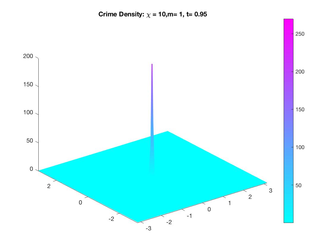
(b) $t=.95$

Figure 1: Numerical solutions with $m=1,\;\chi=10$ and $u_{0}(x)=v_{0}(x)=\frac{1}{\sqrt{2\pi\sigma^{2}}}e^{-\frac{|x|^{2}}{2\sigma^{2}}}$ with $\sigma=1/4$.

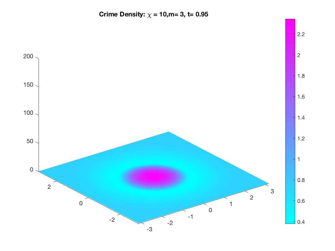
(a) $t=.95$

(b) $t=1.2$

(c) $t=1.95$

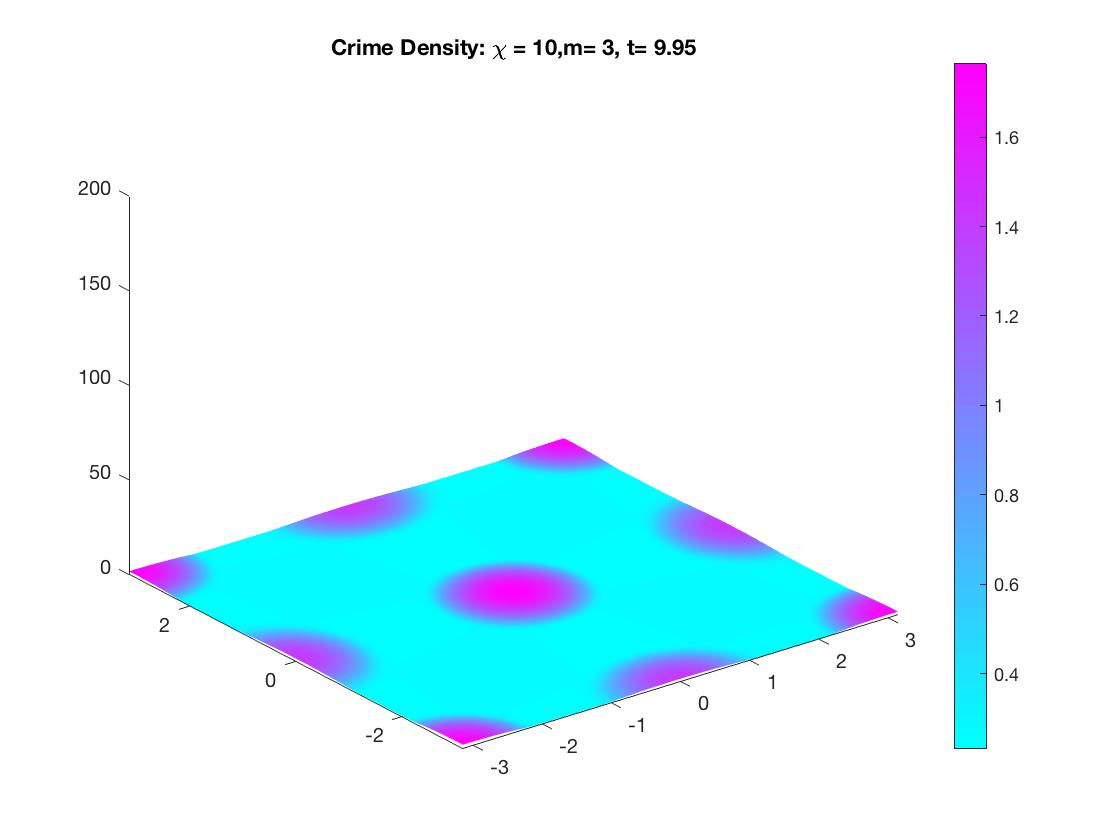
(d) $t=9.95$

Figure 2: Numerical solutions with $m=3,\;\chi=10$ and $u=v=\frac{1}{\sqrt{2\pi\sigma^{2}}}e^{-\frac{|x|^{2}}{2\sigma^{2}}}$ with $\sigma=1/4$.

From more general numerical experiments, we observe that the smaller $\chi$ is, the more concentrated the initial data needs to be in order for a potential blow-up to occur. Moreover, in the case $m=1$, for each $\chi$ there are initial data which are not concentrated enough to see blow-up, but concentrated enough to see initial growth. This initial growth is suppressed by the overcrowding effect seen in (1.3). This is shown in Figure 3 where the top row illustrates the linear diffusion case ($m=1$) and the bottom row illustrates the non-linear diffusion with $m=3$. In the top row we observe the initial growth of the solution in Figure 3b. This growth does not last for very long and the solution is already decaying at time $t=.5$ as illustrated in Figure 3c. We do see some numerical instabilities for the case $m=3$ around the region of concentration. We expect that this is due to the degeneracy of the diffusion and more sophisticated numerical methods need to be used to deal with potential contact lines.

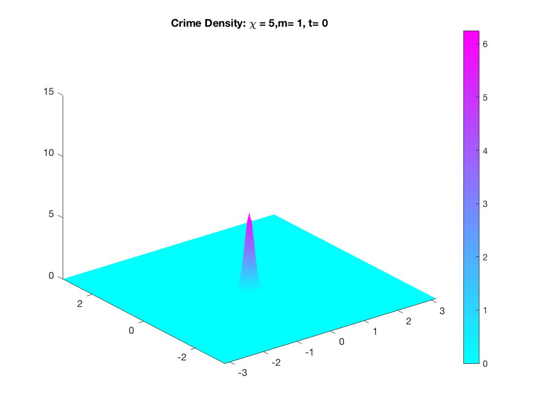
(a) $m=1,\;t=0$

(b) $m=1,\;t=.1$

(c) $m=1,\;t=.5$

(d) $m=3,\;t=0$

(e) $m=3,\;t=.1$

(f) $m=3,\;t=.5$

Figure 3: Numerical solutions comparing $m=1$ and $m=3$ with $\chi=5$ and $u=v=\frac{1}{\sqrt{2\pi\sigma^{2}}}e^{-\frac{|x|^{2}}{2\sigma^{2}}}$ with $\sigma=.16$.

Acknowledgement.  The first author acknowledges support the National Science Foundation, NSF DMS-1516778. The second author acknowledges support of the Deutsche Forschungsgemeinschaft in the context of the project Emergence of structures and advantages in cross-diffusion systems (No. 411007140, GZ: WI 3707/5-1).

References

- [1] H. Amann: Dynamic theory of quasilinear parabolic systems III. Global existence. Math. Z. 202, 219-250 (1989)
- [2] Bellomo, N., Berestycki, H., Brezzi, F., Nadal, J.-P.: Mathematics and complexity in life and human sciences. Math. Mod. Meth. Appl. Sci. 20, 1391-1395 (2010)
- [3] Bellomo, N., Bellouquid, A., Tao, Y., Winkler, M.: Toward a Mathematical Theory of Keller-Segel Models of Pattern Formation in Biological Tissues. Math. Mod. Meth. Appl. Sci. 25, 1663-1763 (2015)
- [4] Felson, M.: Routine activities and crime prevention in the developing metropolis. Criminology 25, 911-932 (1987)
- [5] Freitag, M.: Global solutions to a higher-dimensional system related to crime modeling. Math. Methods Appl. Sci. 41, 6326-6335 (2018)
- [6] Fujie, K.: Study of reaction-diffusion systems modeling chemotaxis. PhD thesis, Tokyo University of Science, 2016
- [7] Heihoff, F.: Generalized solutions for a system of partial differential equation arising from urban crime modeling with a logistic source term. Z. Angew. Math. Phys., to appear
- [8] Herrero, M. A., Velázquez, J. J. L.: A blow-up mechanism for a chemotaxis model. Ann. Scuola Normale Superiore Pisa Cl. Sci. 24, 633-683 (1997)
- [9] Johnson, S.D., Bowers, K., Hirschfeld, A.: New insights into the spatial and temporal distribution of repeat victimisation. British Journal of Criminology 37, 224-241 (1997)
- [10] Porzio, M.M., Vespri, V.: Holder Estimates for Local Solutions of Some Doubly Nonlinear Degenerate Parabolic Equations, J. Differential Eq. 103, 146-178 (1993)
- [11] Rodriguez, N., Winkler, M.: On the global existence and qualitative behavior of one-dimensional solutions to a model for urban crime. Preprint
- [12] Short, M.B., D’Orsogna, M.R., Brantingham, P.J., Tita, G.E.: Measuring and modeling repeat and near-repeat burglary effects. Journal of Quantitative Criminology 25, 325-339 (2009)
- [13] Short, M.B., D’Orsogna, M.R., Pasour, V.B., Tita, G.E., Brantingham, P.J., Bertozzi, A.L., Chayes, L.B.: A statistical model of criminal behavior. Math. Mod. Meth. Appl. Sci. 18 (suppl.), 1249-1267 (2008)
- [14] Short, M.B., Brantingham, P.J., Bertozzi, A.L., Tita, G.E.: Dissipation and displacement of hotspots in reaction-diffusion models of crime. Proc. Nat. Acad. Sci. U.S.A. 107, 3961-3965 (2010)
- [15] Tao, Y., Winkler, M.: Boundedness in a quasilinear parabolic-parabolic Keller-Segel system with subcritical sensitivity. J. Differential Eq. 252, 692-715 (2012)
- [16] Tao, Y., Winkler, M.: Global smooth solutions in a two-dimensional cross-diffusion system modeling urban crime. Preprint
- [17] Temam, R.: Navier-Stokes equations. Theory and numerical analysis. Studies in Mathematics and its Applications. Vol. 2. North-Holland, Amsterdam, 1977
- [18] Winkler, M.: Aggregation vs. global diffusive behavior in the higher-dimensional Keller-Segel model. J. Differential Eq. 248, 2889-2905 (2010)
- [19] Winkler, M: Finite-time blow-up in the higher-dimensional parabolic-parabolic Keller-Segel system. J. Math. Pures Appl. 100, 748-767 (2013), arXiv:1112.4156v1
- [20] Winkler, M: Global solvability and stabilization in a two-dimensional cross-diffusion system modeling urban crime propagation. Ann. Inst. H. Poincaré – Anal. Non Linéaire 36, 1747-1790 (2019)