Learning the gravitational force law and other analytic functions

Abstract

Large neural network models have been successful in learning functions of importance in many branches of science, including physics, chemistry and biology. Recent theoretical work has shown explicit learning bounds for wide networks and kernel methods on some simple classes of functions, but not on more complex functions which arise in practice. We extend these techniques to provide learning bounds for analytic functions on the sphere for any kernel method or equivalent infinitely-wide network with the corresponding activation function trained with SGD. We show that a wide, one-hidden layer ReLU network can learn analytic functions with a number of samples proportional to the derivative of a related function. Many functions important in the sciences are therefore efficiently learnable. As an example, we prove explicit bounds on learning the many-body gravitational force function given by Newton’s law of gravitation. Our theoretical bounds suggest that very wide ReLU networks (and the corresponding NTK kernel) are better at learning analytic functions as compared to kernel learning with Gaussian kernels. We present experimental evidence that the many-body gravitational force function is easier to learn with ReLU networks as compared to networks with exponential activations.

1 Introduction

Despite the empirical success of neural networks and other highly parameterized machine learning methods, a major open question remains: why do these methods perform well? Classical learning theory does not predict or explain the success of large, often overparameterized models (Lawrence et al., 1997; Harvey et al., 2017; Bartlett et al., 2019). Most models are highly expressive (Poole et al., 2016; Raghu et al., 2017), but can still generalize when trained with many less data points than parameters (He et al., 2016; Szegedy et al., 2016; Dai et al., 2019).

In particular, many functions of importance to physics (Mills et al., 2017; Gao & Duan, 2017; Carrasquilla & Melko, 2017; Raissi & Karniadakis, 2018), chemistry (Rupp et al., 2012; Faber et al., 2017), and biology (Kosciolek & Jones, 2016; Ainscough et al., 2018; Xu, 2019), among other fields, can be learned using neural networks and kernel methods. This leads to the question: can we understand what types of functions can be learned efficiently with particular methods? Recent theoretical work has focused on answering this question by constructing bounds on the generalization error, given properties of the model and data distribution. Specifically, for very wide networks with specific kernels or activations (Jacot et al., 2018; Du et al., 2019; Allen-Zhu et al., 2019; Arora et al., 2019; Lee et al., 2019), data-dependent generalization bounds can be derived by relating wide networks to kernel learning with a specific network-induced kernel, known as the neural tangent kernel (NTK) (Jacot et al., 2018). These bounds while not tight, can be used to mathematically justify why neural networks trained on noisy labels can achieve low training error but will fail to generalize, while those trained on real data generalize well. It is unclear, however, whether they give a sense of the relative difficulty of learning different types of functions with different types of methods.

1.1 Our contributions

To explain and further understand the efficacy of deep learning in numerous applications, we present generalization bounds on learning analytic functions on the unit sphere with any kernel method or sufficiently wide neural network (Section 3.1). In the particular case of a wide, one-hidden layer ReLU network, we present a succinct bound on the number of samples needed to guarantee low test error. Informally, we prove the following:

Theorem 1.1 (informal).

Given an analytic function $g(y)$, the function $g(\boldsymbol{\beta}\cdot\mathbf{x})$, for fixed $\boldsymbol{\beta}\in\mathbb{R}^{d}$ and inputs $\mathbf{x}\in\mathbb{R}^{d}$ is learnable to error $\epsilon$ with $O((\beta\tilde{g}^{\prime}(\beta)+\tilde{g}(0))^{2}/\epsilon^{2})$ samples, with

$$\tilde{g}(y)=\sum_{k=0}^{\infty}|a_{k}|x^{k}$$ (1)

where the $a_{k}$ are the power series coefficients of $g(y)$.

We prove a much more general version for multivariate analytic functions:

Theorem 1.2 (informal).

Given a multivariate analytic function $g(\mathbf{x})$ for $\mathbf{x}$ in the $d$-dimensional unit ball, there is a function $\tilde{g}(y)$ as defined in Theoreom 1.1 such that $g(\mathbf{x})$ is learnable to error $\epsilon$ with $O(\tilde{g}^{\prime}(1)/\epsilon^{2})$ samples.

Using Theorem 1.2, we develop a calculus of bounds - showing that the sum, product, and composition of learnable functions is also learnable, with bounds constructed using the familiar product and chain rules of univariate calculus (Corollaries 1.1, 1.2, and 1.3). These bounds also can be applied when $g(\mathbf{x})$ has a singularity, provided that the data is sampled away from the singularity.

Since many functions used in scientific theories and models fall into this function class, our calculus allows for a clear quantifiable explanation for why neural network models have had successful applications to many of those fields. As an important example from physics, we consider the forces $\{\mathbf{F}_{i}\}$ between $k$ bodies with positions $\mathbf{x}_{i}$ interacting via Newtonian gravitation:

$$\mathbf{F}_{i}=\sum_{j\neq i}\frac{m_{i}m_{j}}{||\mathbf{x}_{i}-\mathbf{x}_{j}||^{3}}(\mathbf{x}_{j}-\mathbf{x}_{i})$$ (2)

We show that, as long as there is some minimum distance between the $\mathbf{x}_{i}$ and $\mathbf{x}_{j}$, we can still use the calculus of bounds to show that the $k$ force vectors can be efficiently learned. We prove the following:

Theorem 2 (informal).

A wide, one-hidden layer ReLU network can learn the force law between $k$ gravitational bodies up to error $\epsilon$ using only $k^{O(\ln(k^{2}/\epsilon))}$ samples.

Lastly, we compare our generalization bounds for the ReLU network with those for more traditional kernel learning methods. Specifically, we show asymptotically weaker bounds for other models, including for kernel regression with Gaussian kernels, providing some theoretical evidence why neural networks with ReLU activation (or their induced kernels) often achieve superior performance than the standard Gaussian kernels. We support our theoretical work with numerical experiments on a synthetic dataset that show that wide networks can learn the gravitational force law with minimal fine-tuning, and achieve lower test and generalization error than the standard Gaussian kernel counterpart. Our results suggest that networks with better theoretical learning bounds may in fact perform better in practice as well, even when theoretical bounds are pessimistic.

2 Prelimaries

2.1 Background

Classical tools like VC dimension (Vapnik, 2000) are insufficient to explain the performance of overparameterized neural networks (Bartlett et al., 2019). Networks generalize well even though are often very expressive (Poole et al., 2016; Raghu et al., 2017), can memorize random data (Zhang et al., 2017; Arpit et al., 2017), and have correspondingly large VC dimensions (Maass, 1994; Harvey et al., 2017; Bartlett et al., 2019).

Some progress has been made by focusing on the “implicit regularization” provided by training dynamics (Gunasekar et al., 2018; Du & Lee, 2018; Arora et al., 2018). In particular, SGD biases networks to solutions with small weight changes under the $\ell_{2}$ norm (plus any additional regularization), which has been used to inspire various norm-based bounding strategies (Neyshabur et al., 2018; Allen-Zhu et al., 2019; Arora et al., 2019). While many of these bounds must be computed post-training, some bounds can be computed using the architecture alone, and show that function classes like outputs of small networks with smooth activations can be efficiently learned with large networks (Allen-Zhu et al., 2019; Arora et al., 2019; Du et al., 2019).

Recently, learning bounds for very wide networks have been derived by combining insights on learning dynamics with more classical generalization error bounds in kernel learning. In the limit of infinite width, the total change in each individual parameter is small, and the outputs of the network are linear in the weight changes and it can be shown that the learning dynamics are largely governed by the neural tangent kernel (NTK) of the corresponding network (Jacot et al., 2018). Given the $n\times 1$ dimensional vector $\hat{\mathbf{y}}(\boldsymbol{\theta})$ of model outputs on the training data, as a function of trainable parameters $\boldsymbol{\theta}$, the empirical tangent kernel is the $n\times n$ matrix given by

$$\mathbf{H}=\frac{\partial\mathbf{y}}{\partial\boldsymbol{\theta}}\left(\frac{\partial\mathbf{y}}{\partial\boldsymbol{\theta}}\right)^{{\rm T}}$$ (3)

Since the derivatives are only taken with respect to the parameters that are trained, the tangent kernel is different if particular layers of the network are fixed after initialization. The empirical kernel concentrates around some limiting matrix $\mathbf{H}^{\infty}$ in the limit of a large number of parameters. The NTK kernel evaluated on two inputs $\mathbf{x},\mathbf{x}^{\prime}$ corresponds to the limiting value of $\mathbf{H}^{\infty}$ evaluated at $\mathbf{x}$ and $\mathbf{x}^{\prime}$.

As an example, the kernel function $K(\mathbf{x},\mathbf{x}^{\prime})$ for inputs $\mathbf{x}$ and $\mathbf{x}^{\prime}$ into a single hidden layer fully-connected network, with non-linearity $\phi$, with only final layer weights trained is (Jacot et al., 2018; Lee et al., 2019)

$$K(\mathbf{x},\mathbf{x}^{\prime})={\rm E}[\phi(\mathbf{x}\cdot\mathbf{z})\phi(\mathbf{x}^{\prime}\cdot\mathbf{z})]$$ (4)

where the $\mathbf{z}_{i}$ are i.i.d. Gaussian random variables with the same variance $\sigma^{2}$ as the hidden layer weights. Note here that $H$ is a function of $\mathbf{x}\cdot\mathbf{x}$, $\mathbf{x}\cdot\mathbf{x}^{\prime}$ and $\mathbf{x}^{\prime}\cdot\mathbf{x}^{\prime}$ only.

With MSE loss, the learning dynamics in the wide network regime is similar to kernel regression or kernel learning. Rademacher complexity (Koltchinskii & Panchenko, 2000) can be used to generate learning bounds for wide networks near the infinite width limit, such as in (Arora et al., 2019). The following theorem shows that if for training labels $\mathbf{y}$, the product $\mathbf{y}^{{\rm T}}(\mathbf{H}^{\infty})^{-1}\mathbf{y}$ is bounded by $M_{g}$, then wide networks trained with SGD have error less than $\epsilon$ when trained with $O(M_{g}/\epsilon^{2})$ samples:

Theorem ((Arora et al., 2019), 3.3).

Let $g(\mathbf{x})$ be a function over $\mathbb{R}^{d}$, and $\mathcal{D}$ be a distribution over the inputs. Let $\mathcal{L}$ be a 1-Lipschitz loss function. Consider training a two-layer ReLu network to learn $g$ using SGD with MSE loss on $n$ i.i.d. samples from $\mathcal{D}$. Define the generalization error $E_{gen}$ of the trained model $\hat{g}(\mathbf{x})$ as

$$E_{gen}={\rm E}_{\mathbf{x}\sim\mathcal{D}}[\mathcal{L}(g(\mathbf{x}),\hat{g}(\mathbf{x}))]$$ (5)

Fix a failure probability $\delta$. Suppose that with probability greater than $\delta/3$, $\mathbf{H}^{\infty}$ has smallest eigenvalue $\lambda_{0}>0$. Then for a wide enough network, with probability at least $1-\delta$, the generalization error is at most

$$E_{gen}\leq\sqrt{\frac{2\mathbf{y}^{{\rm T}}(\mathbf{H}^{\infty})^{-1}\mathbf{y}}{n}}+O\left(\sqrt{\frac{\log(n/\lambda_{0}\delta)}{n}}\right)$$ (6)

where $\mathbf{H}^{\infty}$ is the $n\times n$ Gram matrix whose elements correspond to the NTK kernel evaluated at pairs of the $n$ i.i.d. training examples, and $\mathbf{y}$ is the $n$-dimensional vector of training labels.

If there is some $n$-independent constant $M_{g}$ such that $\mathbf{y}^{{\rm T}}(\mathbf{H}^{\infty})^{-1}\mathbf{y}\leq M_{g}$, then with probability at least $1-\delta$, $O([M_{g}+\log(\delta^{-1})]/\epsilon^{2})$ samples are sufficient to ensure generalization error less than $\epsilon$.

2.2 Notation

We define $\|\cdot\|$ to be the Euclidean norm, unless otherwise specified and $\mathbf{x}\cdot\mathbf{x}^{\prime}$ to be the dot product between vectors $\mathbf{x},\mathbf{x}^{\prime}$. For a vector $\mathbf{x}$ and a scalar $c$, we define $\mathbf{x}+c=\mathbf{x}+c{\bf 1}$ and other operations analogously. For the remainder of this paper, we focus on the learnability of functions under different learning algorithms and so we will define efficiently learnable functions as:

Definition 1.

Given a learning algorithm, we say that a function $g$ over a distribution of inputs $\mathcal{D}$ is efficiently learnable if, given an error scale $\epsilon$, with probability greater than $1-\delta$, the generalization error ${\rm E}_{\mathbf{x}\sim\mathcal{D}}[\mathcal{L}(g(\mathbf{x}),\hat{g}(\mathbf{x}))]$ of the trained model $\hat{g}$ with respect to any 1-Lipschitz loss function $\mathcal{L}$ is less than $\epsilon$ when the training data consists of at least $O([M_{g}+\log(\delta^{-1})]/\epsilon^{2})$ i.i.d. samples drawn from $\mathcal{D}$, for some $n$-independent constant $M_{g}$.

3 Theory

3.1 Kernel learning bounds

In this section, we extend the bounds derived in (Arora et al., 2019) to any kernel that can be written as a power series in the dot product of inputs $\mathbf{x}\cdot\mathbf{x}^{\prime}$. We emphasize that our kernel learning bounds can be generalized to the setting where we train a wide neural network on our data. In Appendix A, we make this relation rigorously clear and show that Equation 6 applies when training the upper layer only of any wide network - which is equivalent to a draw from the posterior of a Gaussian process with the NTK kernel given by Equation 4. Therefore, we focus on kernels in this section.

We can extend the following corollary, originally proved for wide ReLU networks with trainable hidden layer only:

Corollary ((Arora et al., 2019), 6.2).

Consider the function $g:\mathbb{R}^{d}\to\mathbb{R}$ given by:

$$g(\mathbf{x})=\sum_{k}a_{k}(\boldsymbol{\beta}_{k}^{{\rm T}}\mathbf{x})^{k}$$ (7)

Then, if $g$ is restricted to $||\mathbf{x}||=1$, and the NTK kernel can be written as $H(\mathbf{x},\mathbf{x}^{\prime})=\sum_{k}b_{k}(\mathbf{x}\cdot\mathbf{x}^{\prime})^{k}$, the function can be learned efficiently with a wide one-hidden-layer network in the sense of Definition 1 with

$$\sqrt{M_{g}}=\sum_{k}b_{k}^{-1/2}|a_{k}|||\boldsymbol{\beta}_{k}||_{2}^{k}$$ (8)

up to $g$-independent constants of $O(1)$, where $\beta_{k}\equiv||\boldsymbol{\beta}_{k}||_{2}$. In the particular case of a ReLU network, the bound is

$$\sqrt{M_{g}}=\sum_{k}k|a_{k}|||\boldsymbol{\beta}_{k}||_{2}^{k}$$ (9)

if the $a_{k}$ are non-zero only for $k=1$ or $k$ even.

Using Equation 6 and the arguments of Appendix A, we arrive at the following extension:

Extension of Corollary ((Arora et al., 2019), 6.2).

Consider a kernel method or appropriately wide network with only the upper layer trained, with kernel

$$K(\mathbf{x},\mathbf{x}^{\prime})=\sum_{k}b_{k}(\mathbf{x}\cdot\mathbf{x}^{\prime})^{k}$$ (10)

Then the learning bound in Equation 8 holds for these models as well.

Building off of this learning bound, we will prove in Section 3.2 that all analytic functions are efficiently learnable, via both kernel methods and wide networks.

Equation 8 suggests that kernels with slowly decaying (but still convergent) $b_{k}$ will give the best bounds for learning polynomials. Many popular kernels do not meet this criteria. For example, for inputs on the sphere of radius $r$, the Gaussian kernel $K(\mathbf{x},\mathbf{x}^{\prime})=e^{-||\mathbf{x}-\mathbf{x}^{\prime}||^{2}/2}$ can be written as $K(\mathbf{x},\mathbf{x}^{\prime})=e^{-r^{2}}e^{\mathbf{x}\cdot\mathbf{x}^{\prime}}$. This has $b_{k}^{-1/2}=e^{r^{2}/2}\sqrt{k!}$, which increases rapidly with $k$. This provides theoretical justification for the empirically inferior performance of the Gaussian kernel which we will present in Section 4.

Guided by this theory, we focus on kernels where $b_{k}^{-1/2}\leq O(k)$, for all $k$. While the ReLU NTK kernel (with inputs on the sphere) satisfies this bound for even positive powers $k$, it fails to satisfy our criteria for odd values of $k$. One way to ensure the bound exists for all $k>0$ is to construct a kernel by hand: for example,

$$K(\mathbf{x},\mathbf{x}^{\prime})=\sum_{k}k^{-s}(\mathbf{x}\cdot\mathbf{x}^{\prime})^{k}$$ (11)

with $s\in(1,2]$ is a valid slowly decaying kernel on the sphere.

Another approach, which keeps the model similar to those used in practice, is to introduce a novel kernel by applying the following modification to the NTK kernel. Consider appending a constant component to the input $\mathbf{x}$ so that the new input to the network is $(\mathbf{x}/\sqrt{2},1/\sqrt{2})$. The kernel then becomes:

$$K(\mathbf{x},\mathbf{x}^{\prime})=\frac{\mathbf{x}\cdot\mathbf{x}^{\prime}+1}{4\pi}\left(\pi-\arccos\left(\frac{\mathbf{x}\cdot\mathbf{x}^{\prime}+1}{2}\right)\right)$$ (12)

Re-writing the power series as an expansion around $\mathbf{x}\cdot\mathbf{x}^{\prime}=0$, we have terms of all powers. An asymptotic analysis of the coefficients (Appendix B.1) shows that coefficients $b_{k}$ are asymptotically $O(k^{-3/2})$ - meeting our needs. In particular, this means that the bound in Equation 9 applies to these kernels, without restriction to even $k$. Note that for $k=0$, the constant function $g(\mathbf{x})=a_{0}$ can be learned with $\sqrt{M_{g}}=|a_{0}|$ samples.

3.2 Learning analytic functions

For the remainder of this section, we assume that we are using a GP/wide network with a kernel $K$ of the form $K(\mathbf{x},\mathbf{x}^{\prime})=\sum_{k=0}^{\infty}b_{k}(\mathbf{x}\cdot\mathbf{x}^{\prime})^{k}$. Unless otherwise noted, we also assume that $b_{k}\geq k^{-2}$ for large $k$ so Equation 9 applies for all powers of $k$. We will use this to show that all univariate analytic functions are efficiently learnable, and then extend the results to multivariate functions.

Analytic functions are a rich class with a long history of use in the sciences and applied mathematics. Functions are analytic if they have bounded derivatives of all orders when extended to the complex plane. This is equivalent to having a locally convergent power series representation, a fact which we will exploit for many of our proofs.

3.2.1 Univariate analytic functions

We start with the univariate case and first prove the following:

Theorem 1.1.

Let $g(y)$ be a function analytic around $0$, with radius of convergence $R_{g}$. Define the auxiliary function $\tilde{g}(y)$ by the power series

$$\tilde{g}(y)=\sum_{k=0}^{\infty}|a_{k}|y^{k}$$ (13)

where the $a_{k}$ are the power series coefficients of $g(y)$. Then the function $g(\boldsymbol{\beta}\cdot\mathbf{x})$, for some fixed vector $\boldsymbol{\beta}\in\mathbb{R}^{d}$ with $||\mathbf{x}||=1$ is efficiently learnable in the sense of Definition 1 using a model with the slowly decaying kernel $K$ with

$$\sqrt{M_{g}}=\beta\tilde{g}^{\prime}(\beta)+\tilde{g}(0)$$ (14)

if the norm $\beta\equiv||\boldsymbol{\beta}||_{2}$ is less than $R_{g}$.

Proof.

We first note that the radius of convergence of the power series of $\tilde{g}(y)$ is also $R_{g}$ since $g(y)$ is analytic. Applying Equation 9, pulling out the $0$th order term, and factoring out $\beta$, we get

$$\sqrt{M_{g}}=|a_{0}|+\beta\sum_{k=1}^{\infty}k|a_{k}|\beta^{k}=\beta\tilde{g}^{\prime}(\beta)+\tilde{g}(0)$$ (15)

since $\beta<R_{g}$. ∎

The relationship between $\tilde{g}(y)$ and the original $g(y)$ depends on the power series representation of $g(y)$. For example, for $g(y)=1/(1-y)$, the power series has all positive coefficients and $g(y)=\tilde{g}(y)$. The worst case scenario is when the power series has alternating sign; for example, for $g(y)=e^{-y^{2}}$, $\tilde{g}(y)=e^{y^{2}}$.

3.2.2 Multivariate analytic functions

The above class of efficiently learnable functions is somewhat limiting; it is “closed” over addition (the sum of learnable functions is learnable), but not over products and composition. The following lemma, proved in Appendix B.2, allows us to generalize:

Lemma 1.

Given a collection of $p$ vectors $\boldsymbol{\beta}_{i}$ in $\mathbb{R}^{d}$, the function $f(\mathbf{x})=\prod_{i=1}^{p}\boldsymbol{\beta}_{i}\cdot\mathbf{x}$ is efficiently learnable with

$$\sqrt{M_{f}}=p\prod_{i}\beta_{i}$$ (16)

where $\beta_{i}\equiv||\boldsymbol{\beta}_{i}||_{2}$.

Using this lemma we can prove:

Theorem 1.2.

Let $g(\mathbf{x})$ be a function with multivariate power series representation:

$$g(\mathbf{x})=\sum_{k}\sum_{v\in V_{k}}a_{v}\prod_{i=1}^{k}(\boldsymbol{\beta}_{v,i}\cdot\mathbf{x})$$ (17)

where the elements of $V_{k}$ index the $k$th order terms of the power series. We define $\tilde{g}(y)=\sum_{k}\tilde{a}_{k}y^{k}$ with coefficients

$$\tilde{a}_{k}=\sum_{v\in V_{k}}|a_{v}|\prod_{i=1}^{k}\beta_{v,i}$$ (18)

If the power series of $\tilde{g}(y)$ converges at $y=1$ then with high probability $g(\mathbf{x})$ can be learned efficiently in the sense of Definition 1 with $\sqrt{M_{g}}=\tilde{g}^{\prime}(1)+\tilde{g}(0)$.

Proof.

Follow the construction in Theorem 1.1, using Lemma 1 to get bounds on the individual terms. Then sum and evaluate the power series of $\tilde{g}^{\prime}(1)$ to arrive at the bound. ∎

Since the set of efficiently learnable functions is now appropriately “closed” over addition and multiplication, the standard machinery of calculus can be used to prove learning bounds for combinations of functions with known bounds. For example, we have:

Corollary 1.1 (Product rule).

Let $g(\mathbf{x})$ and $h(\mathbf{x})$ meet the conditions of Theorem 1. Then the product $g(\mathbf{x})h(\mathbf{x})$ is efficiently learnable as well, with bound

$$\sqrt{M_{gh}}=\tilde{g}^{\prime}(1)\tilde{h}(1)+\tilde{g}(1)\tilde{h}^{\prime}(1)+\tilde{g}(0)\tilde{h}(0)$$ (19)

Proof.

Consider the power series of $g(\mathbf{x})h(\mathbf{x})$, which exists and is convergent since each individual series exists and is convergent. Let the elements of $V_{j,g}$ and $V_{k,h}$ index the $j$th order terms of $g$ and the $k$th order terms of $h$ respectively. The individual terms in the series look like:

$$a_{v}b_{w}\prod_{j^{\prime}=1}^{j}(\boldsymbol{\beta}_{v,j^{\prime}}\cdot\mathbf{x})\prod_{k^{\prime}=1}^{k}(\boldsymbol{\beta}_{w,k^{\prime}}\cdot\mathbf{x})~{}\text{for}~{}v\in V_{j,g},~{}w\in V_{k,h}$$ (20)

with bound

$$(j+k)|a_{v}||b_{w}|\prod_{j^{\prime}=1}^{j}\beta_{v,j^{\prime}}\prod_{k^{\prime}=1}^{k}\beta_{w,k^{\prime}}~{}\text{for}~{}v\in V_{j,g},~{}w\in V_{k,h}$$ (21)

for all terms with $j+k>0$ and $\tilde{g}(0)\tilde{h}(0)$ for the term with $j=k=0$.

Distribute the $j+k$ product, and first focus on the $j$ term only. Summing over all the $V_{k,h}$ for all $k$, we get

$$\begin{split}\sum_{k}\sum_{w\in V_{k,h}}j|a_{v}||b_{w}|\prod_{j^{\prime}=1}^{j}\beta_{v,j^{\prime}}\prod_{k^{\prime}=1}^{k}\beta_{w,k^{\prime}}&=\\ |a_{v}|\prod_{j^{\prime}=1}^{j}\beta_{v,j^{\prime}}\tilde{h}(1)\end{split}$$ (22)

Now summing over the $j$ and $V_{j,g}$ we get $\tilde{g}^{\prime}(1)\tilde{h}(1)$. If we do the same for the $k$ term, after summing we get $\tilde{g}(1)\tilde{h}^{\prime}(1)$. These bounds add and we get the desired formula for $\sqrt{M_{gh}}$, which, up to the additional $\tilde{g}(0)\tilde{h}(0)$ term looks is the product rule applied to $\tilde{g}$ and $\tilde{h}$. ∎

One immediate application for this corollary is the product of many univariate analytic functions. If we define

$$G(\mathbf{x})=\prod_{i}g_{i}(\boldsymbol{\beta}_{i}\cdot\mathbf{x})$$ (23)

where each of the corresponding $\tilde{g}_{i}(y)$ have the appropriate convergence properties, then $G$ is efficiently learnable with bound $M_{G}$ given by

$$\sqrt{M_{G}}=\left.\frac{d}{dy}\prod_{i}\tilde{g}_{i}(\beta_{i}y)\right|_{y=1}+\prod_{i}\tilde{g}_{i}(0)$$ (24)

We can also derive the equivalent of the chain rule for function composition:

Corollary 1.2 (Chain rule).

Let $g(y)$ be an analytic function and $h(\mathbf{x})$ be efficiently learnable, with auxiliary functions $\tilde{g}(y)$ and $\tilde{h}(y)$ respectively. Then the composition $g(h(\mathbf{x}))$ is efficiently learnable as well with bound

$$\sqrt{M_{g\circ h}}=\tilde{g}^{\prime}(\tilde{h}(1))\tilde{h}^{\prime}(1)+\tilde{g}(\tilde{h}(0))$$ (25)

provided that $\tilde{g}(\tilde{h}(0))$ and $\tilde{g}(\tilde{h}(1))$ converge (equivalently, if $\tilde{h}(0)$ and $\tilde{h}(1)$ are in the radius of convergence of $g$).

Proof.

Writing out $g(h(\mathbf{x}))$ as a power series in $h(\mathbf{x})$, we have:

$$g(h(\mathbf{x}))=\sum_{k=0}^{\infty}a_{k}(h(\mathbf{x}))^{k}$$ (26)

We can bound each term individually, and use the $k$-wise product rule to bound each term of $(h(\mathbf{x}))^{k}$. Doing this, we have:

$$\sqrt{M_{g\circ h}}=\sum_{k=1}^{\infty}k|a_{k}|\tilde{h}^{\prime}(1)\tilde{h}(1)^{k-1}+\sum_{k=0}^{\infty}|a_{k}|\tilde{h}(0)^{k}$$ (27)

Factoring out $\tilde{h}^{\prime}(1)$ from the first term and then evaluating each of the series gets us the desired result. ∎

The chain rule bound be generalized to a $2$-dimensional outermost function $f(x,y)$, as proved in Appendix C:

Corollary 1.3.

Let $f(x,y)$ be analytic, with $\tilde{f}(x,y)$ be the function obtained by taking the multivariate power series of $f$ and replacing all coefficients with their absolute values. Then, if $g(\mathbf{x})$ and $h(\mathbf{x})$ are both efficiently learnable, $f(g(\mathbf{x}),h(\mathbf{x}))$ is as well with bound

$$\sqrt{M_{f\circ(g,h)}}=\left.\frac{d}{dy}\tilde{f}(\tilde{g}(y),\tilde{h}(y))\right|_{y=1}$$ (28)

provided $\tilde{f}(\tilde{g}(y),\tilde{h}(y))$ converges at $y=1$.

3.3 Learning dynamical systems

We can use the product and chain rules to show that many functions important in scientific applications can be efficiently learnable. This is true even when the function has a singularity. As an example demonstrating both, we prove the following bound on learning Newton’s law of gravitation:

Theorem 2.

Consider a system of $k$ bodies with positions $\mathbf{x}_{i}\in\mathbb{R}^{3}$ and masses $m_{i}$, interacting via the force:

$$\mathbf{F}_{i}=\sum_{j\neq i}\frac{m_{i}m_{j}}{r_{ij}^{3}}(\mathbf{x}_{j}-\mathbf{x}_{i})$$ (29)

where $r_{ij}\equiv||\mathbf{x}_{i}-\mathbf{x}_{j}||$. We assume that $R=r_{max}/r_{min}$, the ratio between the largest and smallest pairwise distance between any two bodies, is constant. Suppose the $m_{i}$ have been rescaled to be between $0$ and $1$. Then the force law is efficiently learnable in the sense of Definition 1 using the modified ReLU kernel to generalization error less than $\epsilon$ using $k^{O(\ln(k/\epsilon))}$ samples.

Proof.

We will prove learning bounds for each component of $F$ separately, showing efficient learning with probability greater than $1-\delta/3k$. Then, using the union bound, the probability of simultaneously learning all the components efficiently will be $1-\delta$.

There are two levels of approximation: first, we will construct a function which is within $\epsilon/2$ of the original force law, but more learnable. Secondly, we will prove bounds on learning that function to within error $\epsilon/2$.

We first rescale the vector of collective $\{\mathbf{x}_{i}\}$ so that their collective length is at most $1$. In these new units, this gives us $r_{max}^{2}\leq\frac{2}{k}$. The first component of the force on $\mathbf{x}_{1}$ can be written as:

$$(\mathbf{F}_{1})_{1}=\sum_{j=2}^{k}\frac{m_{1}m_{j}}{r_{1j}^{2}}\frac{((\mathbf{x}_{j})_{1}-(\mathbf{x}_{1})_{1})}{r_{1j}}$$ (30)

If we find a bound $\sqrt{M_{f}}$ for an individual contribution $f$ to the force, we can get a bound on the total $\sqrt{M_{F}}=(k-1)\sqrt{M_{f}}$. Consider an individual force term in the sum. The force has a singularity at $r_{1j}=0$. In addition, the function $r_{1j}$ itself is non-analytic due to the branch cut at $0$.

We instead will approximate the force law with a finite power series in $r_{1j}^{2}$, and get bounds on learning said power series. The power series representation of $(1-x)^{-3/2}$ is $\sum_{n=0}^{\infty}\frac{(2n+1)!!}{(2n)!!}x^{n}$. If we approximate the function with $d$ terms, the error can be bounded using Taylor’s theorem. The Lagrange form of the error gives us the bound

$$\left|\frac{1}{(1-x)^{3/2}}-\sum_{n=0}^{d}\frac{(2n+1)!!}{(2n)!!}x^{n}\right|\leq\frac{\sqrt{\pi d}|x|^{d+1}}{(1-|x|)^{5/2+d}}$$ (31)

where we use $\frac{(2n+1)!!}{(2n)!!}\approx\sqrt{\pi n}$ for large $n$. We can use the above expansion by rewriting

$$r_{1j}^{-3}=a^{-3}(1-(1-r_{1j}^{2}/a^{2}))^{-3/2}$$ (32)

for some shift $a$. Approximation with $f_{d}(r_{1j}^{2})$, the first $d$ terms of the power series in $(1-r_{1j}^{2}/a^{2})$ gives us the error:

$$|f_{d}(r_{1j}^{2})-r_{1j}^{-3}|\leq\frac{\sqrt{\pi d}|1-r_{1j}^{2}/a^{2}|^{d+1}}{a^{3}(1-|1-r_{1j}^{2}/a^{2}|)^{5/2+d}}$$ (33)

which we want to be small over the range $r_{min}\leq r_{1j}\leq r_{max}$.

The bound is optimized when it takes the same value at $r_{min}$ and $r_{max}$, so we set $a^{2}=(r_{min}^{2}+r_{max}^{2})/2$. In the limit that $r_{max}\gg r_{min}$, where learning is most difficult, the bound becomes

$$|f_{d}(r_{1j}^{2})-r_{1j}^{-3}|\leq\frac{\sqrt{8\pi d}}{r_{max}^{3}}\left(R^{2}/2\right)^{5/2+d}e^{-2(d+1)/R^{2}}$$ (34)

where $R=r_{max}/r_{min}$, which is constant by assumption.

In order to estimate an individual contribution to the force force to error $\epsilon/2k$ (so the total error is $\epsilon/2$), we must have:

$$m_{1}m_{j}r_{max}|f_{d}(r_{1j})-r_{1j}^{-3}|\leq\frac{\epsilon}{2k}$$ (35)

This allows us to choose the smallest $d$ which gives us this error. Taking the logarithm of both sides, we have:

$$\frac{1}{2}\ln(d)-(5/2+d)\ln\left(2/R^{2}\right)-2(d+1)/R^{2}\leq\ln(\epsilon/k^{2})$$ (36)

where we use that $r_{max}^{2}\leq 2/k$ after rescaling. The choice $d\geq R^{2}\ln(k^{2}/\epsilon)$ ensures error less than $\epsilon/2k$ per term.

Using this approximation, we can use the product and chain rules to get learning bounds on the force law. We can write the approximation

$$F_{\epsilon}(\mathbf{x})=\sum_{j\neq 1}m_{1}m_{j}f_{d}(h_{j}(\mathbf{x}))k_{j}(\mathbf{x})$$ (37)

where $h_{j}(\mathbf{x})=||\mathbf{x}_{1}-\mathbf{x}_{j}||$ and $k_{j}(\mathbf{x})=(\mathbf{x}_{1})_{1}-(\mathbf{x}_{j})_{j}$ The number of samples needed for efficient learning is bounded by $\sqrt{M_{F_{\epsilon}}}=\frac{\sqrt{8}k}{r_{max}^{3}}A_{F_{\epsilon}}$, for

$$A_{F_{\epsilon}}=\tilde{f}_{d}^{\prime}(\tilde{h}(1))\tilde{h}^{\prime}(1)\tilde{k}(1)+\tilde{f}_{d}(\tilde{h}(1))\tilde{k}^{\prime}(1)$$ (38)

with

$$\tilde{k}(y)=\sqrt{2}y,~{}\tilde{h}(y)=6y^{2},~{}\tilde{f}_{d}(y)=\sqrt{\pi d}(1+y/a^{2})^{d}$$ (39)

Evaluating, we have

$$A_{F_{\epsilon}}=\sqrt{2\pi d}\left(1+\frac{12}{r_{max}^{2}}\right)^{d}+\sqrt{\pi d^{3}}\left(1+\frac{12}{r_{max}^{2}}\right)^{d-1}$$ (40)

which, after using $r_{max}^{2}\leq 2/k$ and $d=R^{2}\ln(k^{2}/\epsilon)$ gives us the bound

$$\sqrt{M_{F_{\epsilon}}}\leq k^{-1/2}\left(R^{2}\ln(k^{2}/\epsilon)\right)^{3/2}\left(24k\right)^{R^{2}\ln(k^{2}/\epsilon)}$$ (41)

The asymptotic behavior is

$$\sqrt{M_{F_{\epsilon}}}=k^{O(\ln(k/\epsilon))}$$ (42)

since $R$ is bounded.

We can therefore learn an $\epsilon/2$-approximation of one component of $\mathbf{F}_{1}$, with probability at least $1-\delta/3k$ and error $\epsilon/2$ with $O(4(M_{F_{\epsilon}}+\log(3k/\delta))/\epsilon^{2})$ samples. Therefore, we can learn $\mathbf{F}_{1}$ to error $\epsilon$ with the same number of samples. Using a union bound, with probability at least $1-\delta$ we can simultaneously learn all components of all $\{\mathbf{F}_{i}\}$ with that number of samples. ∎

We note that since the cutoff of the power series at $d(\epsilon)=O(R^{2}\ln(k^{2}/\epsilon))$ dominates the bound, we can easily compute learning bounds for other power-series kernels as well. If the $d$th power series coefficient of the kernel is $b_{d}$, then the bound on $\sqrt{M_{F_{\epsilon}}}$ is increased by $(d(\epsilon)^{2}b_{d(\epsilon)})^{-1/2}$. For example, for the Gaussian kernel, since $b_{d}^{-1/2}=\sqrt{d!}$, the bound becomes

$$\sqrt{M_{F_{\epsilon}}}=(R^{2}\ln(k^{2}/\epsilon)k)^{O(\ln(k/\epsilon))}$$ (43)

which increases the exponent of $k$ by a factor of $\ln(R^{2}\ln(k^{2}/\epsilon))$.

4 Experiments

We empirically validated our analytical learning bounds by training models to learn the gravitational force function for $k$ bodies (with $k$ ranging from $5$ to $400$) in a $3-$dimensional space. We created synthetic datasets by randomly drawing $k$ points from $[0,1]^{3}$ corresponding to the location of $k$ bodies, and compute the gravitational force (according to Equation 2) on a target body also drawn randomly from $[0,1]^{3}$. To avoid singularities, we ensured a minimum distance of $0.1$ between the target body and the other bodies (corresponding to the choice $R=10$). As predicted by the theory, none of the models learn well if $R$ is not fixed. We randomly drew the masses corresponding to the $k+1$ bodies from $[0,10]$. We generated $5$ million such examples - each example with $4(k+1)$ features corresponding to the location and mass of each of the bodies, and a single label corresponding to the gravitational force $F$ on the target body along the $x$-axis. We held out $10\%$ of the dataset as test data to compute the root mean square error (RMSE) in prediction. We trained three different neural networks on this data, corresponding to various kernels we analyzed in the previous section:

1. A wide one hidden-layer ReLU network (corresponding to the ReLU NTK kernel).

2. A wide one hidden-layer ReLU network with a constant bias feature added to the input (corresponding to the NTK kernel in Equation 12).

3. A wide one hidden-layer network with exponential activation function, where only the top layer of the network is trained (corresponding to the Gaussian kernel).

We used a hidden layer of width $1000$ for all the networks, as we observed that increasing the network width further did not improve results significantly. All the hidden layer weights were initialized randomly.

In Figure 1 we show the the normalized RMSE (RMSE/[$F_{max}-F_{min}$]) for each of the neural networks for different values of the number of bodies $k$.

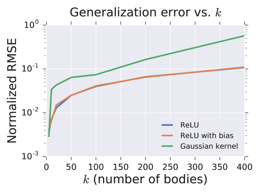
Figure 1: RMSE vs number of bodies $k$ for learning gravitational force law for different kernels. Normalized by the range $F_{max}-F_{min}$ of the forces. Gaussian kernels learn worse than ReLU at large $k$.

All three networks are able to learn the gravitational force equation with small normalized RMSE for hundreds of bodies. Both the ReLU network and ReLU with bias outperform the network corresponding to the Gaussian kernel (in terms of RMSE) as $k$ increases. In particular, the Gaussian kernel learning seems to quickly degrade at around $400$ bodies, with a normalized RMSE exceeding $50\%$. This is consistent with the learning bounds for these kernels in Section 3.1, and suggests that those bounds may in fact be useful to compare the performances of different networks in practice.

We did not, however, observe much difference in the performance of the ReLU network when adding a bias to the input, which suggests that the inability to get an analytical bound due to only even powers in the ReLU NTK kernel might be a shortcoming of the proof technique, rather than a property which fundamentally limits the model.

5 Conclusions

Our theoretical work shows that the broad and important class of analytic functions is provably learnable with the right kernels (or the equivalent wide networks). The methods which we developed may be useful for proving learnability of other classes of functions, such as the flows induced by finite-time integration of differential equations. Furthermore, in general, there is an open question as to whether these generalization bounds can be substantially improved.

Our experiments suggest that these bounds may be useful for distinguishing which types of models are suited for specific problems. Further experimental and theoretical work is necessary to ascertain whether this holds for the finite-width networks used in practice, or when common hyperparameter tuning/regularization strategies are used during training, such as ARD in kernel learning.

Appendix A Kernels and two layer networks

Previous work focused on generalization bounds for training the hidden layers of wide networks with SGD. Here we show that these bounds also apply to the case where only the final layer weights are trained (corresponding to the NNGP kernel in (Lee et al., 2019)). The proof strategy consists of showing that finite-width networks have a sensible infinite-width limit, and showing that training causes only a small change in parameters of the network.

Let $m$ be the number of hidden units, and $n$ be the number of data points. Let $\mathbf{h}$ be a $n\times m$ random matrix denoting the activations of the hidden layer (as a function of the weights of the lower layer) for all $n$ data points. Similarly to (Arora et al., 2019; Du et al., 2019) we will argue that for large enough $m$ even if we take a random input layer and just train the upper layer weights then the generalization error is at most $\sqrt{\frac{\mathbf{y}^{{\rm T}}(\mathbf{H}^{\infty})^{-1}\mathbf{y}}{n}}$. For our purposes, we define:

$$\mathbf{H}^{\infty}={\rm E}[\mathbf{h}\mathbf{h}^{{\rm T}}]$$ (44)

which is the NNGP kernel from (Lee et al., 2019).

If $K(\mathbf{x},\mathbf{x}^{\prime})$, the kernel function which generates $\mathbf{H}^{\infty}$ is given by a infinite Taylor series in $\mathbf{x}\cdot\mathbf{x}^{\prime}$ it can be argued that $\mathbf{H}^{\infty}$ has full rank for most real world distributions. For example, the ReLU activation this holds as long as no two data points are co-linear (see Definition 5.1 in (Arora et al., 2019)). We can prove this more explicitly in the general case.

Lemma 2.

If all the $n$ data points $x$ are distinct and the Taylor series of $K(\mathbf{x},\mathbf{x}^{\prime})$ in $\mathbf{x}\cdot\mathbf{x}^{\prime}$ has positive coefficients everywhere then $\mathbf{H}^{\infty}$ is not singular.

Proof.

First consider the case where the input $x$ is a scalar. Since the Taylor series corresponding to $K(x,x^{\prime})$ consists of monomials of all degrees of $xx^{\prime}$, we can view it as some inner product in a kernel space induced by the function $\Phi(x)=(1,x,x^{2},\ldots)$, where the inner product is diagonal (but with potentially different weights) in this basis. For any distinct set of inputs $\{x_{1},..,x_{n}\}$ the set of vectors $\Phi(x_{i})$ are linearly independent. The first $n$ columns produce the Vandermonde matrix obtained by stacking rows $1,x,x,...,x^{n-1}$ for $n$ different values of $x$, which is well known to be non-singular (since a zero eigenvector would correspond to a degree $n-1$ polynomial with $n$ distinct roots $\{x_{1},..,x_{n}\}$).

This extends to the case of multidimensional $\mathbf{x}$ if the values, projected along some dimension, are distinct. In this case, the kernel space corresponds to the direct sum of copies of $\Phi$ applied elementwise to each coordinate $\mathbf{x}_{i}$. If all the points are distinct and and far apart from each other, the probability that a given pair coincides under random projection is negligible. From a union bound, the probability that a given pair coincide is also bounded – so there must be directions such that projections along that direction are distinct. Therefore, $\mathbf{H}^{\infty}$ can be considered to be invertible in general. ∎

As $m\rightarrow\infty$, $\mathbf{h}\mathbf{h}^{{\rm T}}$ concentrates to its expected value. More precisely, $(\mathbf{h}\mathbf{h}^{{\rm T}})^{-1}$ approaches $(\mathbf{H}^{\infty})^{-1}$ for large $m$ if we assume that the smallest eigenvalue $\lambda_{min}(\mathbf{H}^{\infty})\geq\lambda_{0}$, which from the above lemma we know to be true for fixed $n$. (For the ReLU NTK kernel the difference becomes negligible with high probability for $m=poly(n/\lambda_{0})$ (Arora et al., 2019).) This allows us to replace $\mathbf{h}\mathbf{h}^{{\rm T}}$ with $\mathbf{H}^{\infty}$ in any bounds involving the former.

We can get learning bounds in terms of $\mathbf{h}\mathbf{h}^{{\rm T}}$ in the following manner. The output of the network is given by $\mathbf{y}=\mathbf{w}\cdot\mathbf{h}$, where $\mathbf{w}$ is the vector of upper layer weights and $\mathbf{y}$ is $1\times n$ vector of training output values. The outputs are linear in $\mathbf{w}$. Training only the $\mathbf{w}$, and assuming $\mathbf{h}\mathbf{h}^{{\rm T}}$ is invertible (which the above arguments show is true with high probability for large $m$), the following lemma holds:

Lemma 3.

If we initialize a random lower layer and train the weights of the upper layer, then there exists a solution $\mathbf{w}$ with norm $\mathbf{y}^{{\rm T}}(\mathbf{h}\mathbf{h}^{{\rm T}})^{-1}\mathbf{y}$.

Proof.

The minimum norm solution to $\mathbf{y}=\mathbf{w}^{{\rm T}}\mathbf{h}$ is

$$\mathbf{w}^{*}=(\mathbf{h}^{{\rm T}}\mathbf{h})^{-1}\mathbf{h}^{{\rm T}}\mathbf{y}$$ (45)

The norm $(\mathbf{w}^{*})^{{\rm T}}\mathbf{w}^{*}$ of this solution is given by $\mathbf{y}^{{\rm T}}\mathbf{h}(\mathbf{h}^{{\rm T}}\mathbf{h})^{-2}\mathbf{h}^{{\rm T}}\mathbf{y}$.

We claim that $\mathbf{h}(\mathbf{h}^{{\rm T}}\mathbf{h})^{-2}\mathbf{h}^{{\rm T}}=(\mathbf{h}\mathbf{h}^{{\rm T}})^{-1}$. To show this, consider the SVD decomposition $\mathbf{h}=\mathbf{U}\mathbf{S}\mathbf{V}^{{\rm T}}$. Expanding we have

$$\mathbf{h}(\mathbf{h}^{{\rm T}}\mathbf{h})^{-2}\mathbf{h}^{{\rm T}}=\mathbf{U}\mathbf{S}\mathbf{V}^{{\rm T}}(\mathbf{V}\mathbf{S}^{2}\mathbf{V}^{{\rm T}})^{-2}\mathbf{V}\mathbf{S}\mathbf{U}^{{\rm T}}$$ (46)

Evaluating the right hand side gets us $\mathbf{U}\mathbf{S}^{-2}\mathbf{U}^{{\rm T}}=(\mathbf{h}\mathbf{h}^{{\rm T}})^{-1}$.

Therefore, the norm of the minimum norm solution is $\mathbf{y}^{{\rm T}}(\mathbf{h}\mathbf{h}^{{\rm T}})^{-1}\mathbf{y}$. ∎

For large $m$, the norm approaches $\mathbf{y}^{{\rm T}}(\mathbf{H}^{\infty})^{-1}\mathbf{y}$. Since the lower layer is fixed, the optimization problem is linear and therefore convex in the trained weights $\mathbf{w}$. Therefore SGD with small learning rate will reach this optimal solution. The Rademacher complexity of this function class is at most $\sqrt{\frac{\mathbf{y}^{{\rm T}}(\mathbf{H}^{\infty})^{-1}\mathbf{y}}{2n}}$. The optimal solution has $0$ train error based on the assumption that $\mathbf{H}^{\infty}$ is full rank and the test error will be no more than this Rademacher complexity - identical to the previous results for training a ReLu network (Arora et al., 2019; Du et al., 2019).

Note that although we have argued here assuming only upper layer is trained, (Arora et al., 2019; Du et al., 2019; Andoni et al., 2014) show that even if both layers are trained for large enough $m$ the training dynamics is governed by the NTK kernel, and the lower layer changes so little over the training steps that $\mathbf{h}\mathbf{h}^{{\rm T}}$ remains close to $\mathbf{H}^{\infty}$ through the gradient descent.

Appendix B Learning polynomials with kernels

B.1 Modified ReLU power series

One limitation of the bounds in (Arora et al., 2019) is that they were limited to even-degree polynomials only. One way to overcome that limitation is to compute the NTK kernel of a modified ReLU network. Given an input $\mathbf{x}\in\mathbb{R}^{d}$, the actual input to the vector is the $d+1$ dimensional vector $(\mathbf{x}/\sqrt{2},1/\sqrt{1})$. The resulting kernel is then given by:

$$K(\mathbf{x},\mathbf{x}^{\prime})=\frac{\mathbf{x}\cdot\mathbf{x}^{\prime}+1}{4\pi}\left(\pi-\arccos\left(\frac{\mathbf{x}\cdot\mathbf{x}^{\prime}+1}{2}\right)\right)$$ (47)

for inputs $\mathbf{x}$ and $\mathbf{y}$. We can use the power series of $\arccos$ around $0$ to compute the power series around $\frac{1}{2}$:

$$\begin{split}\pi-&\arccos\left(\frac{x+1}{2}\right)=\\ &\frac{\pi}{2}+\sum_{n=1}^{\infty}\frac{1}{(2n+1)}\frac{(2n-1)!!}{(2n)!!}\left(\frac{1+x}{2}\right)^{2n+1}\end{split}$$ (48)

Evaluating the monomial, we have the double sum

$$\begin{split}\pi-&\arccos\left(\frac{x+1}{2}\right)=\\ &\frac{\pi}{2}+\sum_{n=1}^{\infty}\frac{1}{(2n+1)}\frac{(2n-1)!!}{(2n)!!}\sum_{k=0}^{2n+1}2^{-(2n+1)}\binom{2n+1}{k}x^{k}\end{split}$$ (49)

Let $\sum_{k}b_{k}x^{k}$ be the power series representation about $0$. It is difficult to represent $b_{k}$ in terms of simple functions; nevertheless, we can asymptotically compute the form of $b_{k}$ for large $k$. We have:

$$b_{k}=\sum_{n=1}^{\infty}\frac{1}{(2n+1)}\frac{(2n-1)!!}{(2n)!!}2^{-(2n+1)}\binom{2n+1}{k}$$ (50)

For large $n$ and $k$, using Stirling’s approximation we can write:

$$b_{k}\approx\sum_{n=(k-1)/2}^{\infty}\frac{\sqrt{2}}{\pi}\frac{1}{(2n+1)^{2}}e^{-((2n+1)/2-k)^{2}/(2n+1)}$$ (51)

correct up to multiplicative error $o(1)$. The saddle point approximation gives us that the sum is dominated by terms of order $n=k\pm\sqrt{k}$; therefore the approximate value of the sum is

$$b_{k}\approx\frac{1}{2\sqrt{\pi}}k^{-3/2}$$ (52)

This has the same asymptotic form as the unmodified ReLU kernel without modification, but is now non-zero for odd powers as well. Therefore, the learning bounds from (Arora et al., 2019) (as well as the extension in Lemma 1) will hold for the modified ReLU kernel, for all orders of polynomials.

B.2 Proof of Lemma 1

The following extension of Corollary 6.2 from (Arora et al., 2019) is vital for proving learning bounds on multivariate functions:

Lemma 1.

Given a collection of $p$ vectors $\boldsymbol{\beta}_{i}$ in $\mathbb{R}^{d}$, the function $f(\mathbf{x})=\prod_{i=1}^{p}\boldsymbol{\beta}_{i}\cdot\mathbf{x}$ is efficiently learnable in the sense of Definition 1 using the modified ReLU kernel with

$$\sqrt{M_{f}}=p\prod_{i=1}^{p}\beta_{i}$$ (53)

where $\beta_{i}\equiv||\boldsymbol{\beta}_{i}||_{2}$.

Proof.

The proof of Corollary 6.2 in (Arora et al., 2019) relied on the following statement: given positive semi-definite matrices $\mathbf{A}$ and $\mathbf{B}$, with $\mathbf{A}\succeq\mathbf{B}$, we have:

$$\mathbf{P}_{\mathbf{B}}\mathbf{A}^{-1}\mathbf{P}_{\mathbf{B}}\preceq\mathbf{B}^{+}$$ (54)

where $+$ is the Moore-Penrose pseudoinverse, and $\mathbf{P}$ is the projection operator.

We can use this result, along with the Taylor expansion of the kernel and a particular decomposition of a multivariate monomial in the following way. Let the matrix $\mathbf{X}$ to be the training data, such that the $\alpha$th column $\mathbf{x}_{i}$ is a unit vector in $\mathbb{R}^{d}$. Given $\mathbf{K}\equiv\mathbf{X}^{{\rm T}}\mathbf{X}$, the matrix of inner products, the Gram matrix $\mathbf{H}^{\infty}$ of the kernel can be written as

$$\mathbf{H}^{\infty}=\sum_{k=0}^{\infty}b_{k}\mathbf{K}^{\circ k}$$ (55)

where $\circ$ is the Hadamard (elementwise) product. Consider the problem of learning the function $f(\mathbf{x})=\prod_{i=1}^{p}\boldsymbol{\beta}_{i}\cdot\mathbf{x}$. Note that we can write:

$$f(\mathbf{X})=(\mathbf{X}^{\odot k})^{{\rm T}}\otimes_{i=1}^{k}\boldsymbol{\beta}_{i}$$ (56)

Here $\otimes$ is the tensor product, which for vectors takes an $n_{1}$-dimensional vector and an $n_{2}$ dimensional vector as inputs vectors and returns a $n_{1}n_{2}$ dimensional vector:

$$\mathbf{w}\otimes\mathbf{v}=\begin{pmatrix}w_{1}v_{1}\\ w_{1}v_{2}\\ \cdots\\ w_{1}v_{n_{2}}\\ w_{2}v_{1}\\ \cdots\\ w_{n_{1}}v_{n_{2}}\end{pmatrix}$$ (57)

The operator $\odot$ is the Khatri-Rao product, which takes an $n_{1}\times n_{3}$ matrix $\mathbf{A}=(\mathbf{a}_{1},\cdots,\mathbf{a}_{n_{3}})$ and a $n_{2}\otimes n_{3}$ matrix $\mathbf{B}=(\mathbf{b}_{1},\cdots,\mathbf{b}_{n_{3}})$ and returns the $n_{1}n_{2}\times n_{3}$ dimensional matrix

$$\mathbf{A}\odot\mathbf{B}=(\mathbf{a}_{1}\otimes\mathbf{b}_{1},\cdots,\mathbf{a}_{n_{3}}\otimes\mathbf{b}_{n_{3}})$$ (58)

For $p=2$, this form of $f(\mathbf{X})$ can be proved explicitly:

$$(\mathbf{X}^{\odot 2})^{{\rm T}}\boldsymbol{\beta}_{1}\otimes\boldsymbol{\beta}_{2}=\begin{pmatrix}\mathbf{x}_{1}\otimes\mathbf{x}_{1},\cdots,\mathbf{x}_{P}\otimes\mathbf{x}_{P}\end{pmatrix}^{{\rm T}}\boldsymbol{\beta}_{1}\otimes\boldsymbol{\beta}_{2}$$ (59)

The $\alpha$th element of the matrix product is

$$(\mathbf{x}_{\alpha}\otimes\mathbf{x}_{\alpha})\cdot(\boldsymbol{\beta}_{1}\otimes\boldsymbol{\beta}_{2})=(\boldsymbol{\beta}_{1}\cdot\mathbf{x}_{\alpha})(\boldsymbol{\beta}_{2}\cdot\mathbf{x}_{\alpha})$$ (60)

which is exactly $f(\mathbf{x}_{\alpha})$. The formula can be proved for $p>2$ by finite induction.

With this form of $f(\mathbf{X})$, we can follow the steps of the proof in (Arora et al., 2019), which was written for the case where the $\boldsymbol{\beta}_{i}$ were identical:

$$\mathbf{y}^{{\rm T}}(\mathbf{H}^{\infty})^{-1}\mathbf{y}=(\otimes_{i=1}^{p}\boldsymbol{\beta}_{i})^{{\rm T}}\mathbf{X}^{\odot p}(\mathbf{H}^{\infty})^{-1}(\mathbf{X}^{\odot p})^{{\rm T}}\otimes_{i=1}^{p}\boldsymbol{\beta}_{i}$$ (61)

Using Equation 54, applied to $\mathbf{K}^{\circ p}$, we have:

$$\begin{split}\mathbf{y}^{{\rm T}}&(\mathbf{H}^{\infty})^{-1}\mathbf{y}\leq\\ &b_{p}^{-1}(\otimes_{i=1}^{p}\boldsymbol{\beta}_{i})^{{\rm T}}\mathbf{X}^{\odot p}\mathbf{P}_{\mathbf{K}^{\circ p}}(\mathbf{K}^{\circ p})^{+}\mathbf{P}_{\mathbf{K}^{\circ p}}(\mathbf{X}^{\odot p})^{{\rm T}}\otimes_{i=1}^{p}\boldsymbol{\beta}_{i}\end{split}$$ (62)

Since the $\mathbf{X}^{\odot p}$ are eigenvectors of $\mathbf{P}_{\mathbf{K}^{\circ p}}$ with eigenvalue $1$, and $\mathbf{X}^{\odot p}(\mathbf{K}^{\circ p})^{+}(\mathbf{X}^{\odot p})^{{\rm T}}=\mathbf{P}_{\mathbf{X}^{\odot p}}$, we have:

$$\mathbf{y}^{{\rm T}}(\mathbf{H}^{\infty})^{-1}\mathbf{y}\leq b_{p}^{-1}(\otimes_{i=1}^{p}\boldsymbol{\beta}_{i})^{{\rm T}}\mathbf{P}_{\mathbf{X}^{\odot p}}\otimes_{i=1}^{p}\boldsymbol{\beta}_{i}$$ (63)

$$\mathbf{y}^{{\rm T}}(\mathbf{H}^{\infty})^{-1}\mathbf{y}\leq b_{p}^{-1}\prod_{i=1}^{p}\boldsymbol{\beta}_{i}\cdot\boldsymbol{\beta}_{i}$$ (64)

For the modified ReLU kernel, $b_{p}\geq p^{-2}$. Therefore, we have $\sqrt{\mathbf{y}^{{\rm T}}(\mathbf{H}^{\infty})^{-1}\mathbf{y}}\leq\sqrt{M_{f}}$ for

$$\sqrt{M_{f}}=p\prod_{i}\beta_{i}$$ (65)

where $\beta_{i}\equiv||\boldsymbol{\beta}_{i}||_{2}$, as desired. ∎

Appendix C Multi-dimensional analytic functions

In the main text we proved results for analytic functions comprised of composing a univariate analytic function $g(y)$ with a simple multivariate function $h(\mathbf{x})$. However, we can prove bounds for functions comprised of a composition of a multivariate analytic function $f(x,y)$ with efficiently learnable analytic functions $g(\mathbf{x})$ and $h(\mathbf{x})$. More formally, we prove the following:

Corollary 1.3.

Let $f(x,y)$ be analytic, with $\tilde{f}(x,y)$ be the function obtained by taking the multivariate power series of $f$ and replacing all coefficients with their absolute values. Then, if $g(\mathbf{x})$ and $h(\mathbf{x})$ are both efficiently learnable, $f(g(\mathbf{x}),h(\mathbf{x}))$ is as well with bound

$$\sqrt{M_{f\circ(g,h)}}=\left.\frac{d}{dy}\tilde{f}(\tilde{g}(y),\tilde{h}(y))\right|_{y=1}$$ (66)

provided $\tilde{f}(\tilde{g}(y),\tilde{h}(y))$ converges at $y=1$.

Proof.

Expand the power series of representation of $f(g(\mathbf{x}),h(\mathbf{x}))$. Replacing all terms with their absolute values, multiplied by $y^{k}$ for the appropriate power $k$, we get the power series $\tilde{f}(\tilde{g}(y),\tilde{h}(y))$. Replacing the terms in the power series of $f(g(\mathbf{x}),h(\mathbf{x}))$ with their individual bounds, and comparing with the power series representation of $\frac{d}{dy}\tilde{f}(\tilde{g}(y),\tilde{h}(y))$, we arrive at the result. ∎

Generalizations to higher dimensional $f$ proceed similarly.

References

- Ainscough et al. (2018) Ainscough, B. J., Barnell, E. K., Ronning, P., Campbell, K. M., Wagner, A. H., Fehniger, T. A., Dunn, G. P., Uppaluri, R., Govindan, R., Rohan, T. E., Griffith, M., Mardis, E. R., Swamidass, S. J., and Griffith, O. L. A deep learning approach to automate refinement of somatic variant calling from cancer sequencing data. Nature Genetics, 50(12):1735–1743, December 2018. ISSN 1546-1718. doi: 10.1038/s41588-018-0257-y.
- Allen-Zhu et al. (2019) Allen-Zhu, Z., Li, Y., and Liang, Y. Learning and Generalization in Overparameterized Neural Networks, Going Beyond Two Layers. In Advances in Neural Information Processing Systems 32, pp. 6155–6166. Curran Associates, Inc., 2019.
- Andoni et al. (2014) Andoni, A., Panigrahy, R., Valiant, G., and Zhang, L. Learning Polynomials with Neural Networks. In International Conference on Machine Learning, pp. 1908–1916, January 2014.
- Arora et al. (2018) Arora, S., Ge, R., Neyshabur, B., and Zhang, Y. Stronger Generalization Bounds for Deep Nets via a Compression Approach. In International Conference on Machine Learning, pp. 254–263, July 2018.
- Arora et al. (2019) Arora, S., Du, S., Hu, W., Li, Z., and Wang, R. Fine-Grained Analysis of Optimization and Generalization for Overparameterized Two-Layer Neural Networks. In International Conference on Machine Learning, pp. 322–332, May 2019.
- Arpit et al. (2017) Arpit, D., Jastrzębski, S., Ballas, N., Krueger, D., Bengio, E., Kanwal, M. S., Maharaj, T., Fischer, A., Courville, A., Bengio, Y., and Lacoste-Julien, S. A closer look at memorization in deep networks. In Proceedings of the 34th International Conference on Machine Learning - Volume 70, ICML’17, pp. 233–242, Sydney, NSW, Australia, August 2017. JMLR.org.
- Bartlett et al. (2019) Bartlett, P. L., Harvey, N., Liaw, C., and Mehrabian, A. Nearly-tight VC-dimension and Pseudodimension Bounds for Piecewise Linear Neural Networks. Journal of Machine Learning Research, 20(63):1–17, 2019. ISSN 1533-7928.
- Carrasquilla & Melko (2017) Carrasquilla, J. and Melko, R. G. Machine learning phases of matter. Nature Physics, 13(5):431–434, May 2017. ISSN 1745-2481. doi: 10.1038/nphys4035.
- Dai et al. (2019) Dai, Z., Yang, Z., Yang, Y., Carbonell, J., Le, Q., and Salakhutdinov, R. Transformer-XL: Attentive Language Models beyond a Fixed-Length Context. In Proceedings of the 57th Annual Meeting of the Association for Computational Linguistics, pp. 2978–2988, Florence, Italy, July 2019. Association for Computational Linguistics. doi: 10.18653/v1/P19-1285.
- Du & Lee (2018) Du, S. and Lee, J. On the Power of Over-parametrization in Neural Networks with Quadratic Activation. In International Conference on Machine Learning, pp. 1329–1338, July 2018.
- Du et al. (2019) Du, S. S., Zhai, X., Póczos, B., and Singh, A. Gradient Descent Provably Optimizes Over-parameterized Neural Networks. In 7th International Conference on Learning Representations, ICLR 2019, New Orleans, LA, USA, May 6-9, 2019. OpenReview.net, 2019.
- Faber et al. (2017) Faber, F. A., Hutchison, L., Huang, B., Gilmer, J., Schoenholz, S. S., Dahl, G. E., Vinyals, O., Kearnes, S., Riley, P. F., and von Lilienfeld, O. A. Prediction Errors of Molecular Machine Learning Models Lower than Hybrid DFT Error. Journal of Chemical Theory and Computation, 13(11):5255–5264, November 2017. ISSN 1549-9618. doi: 10.1021/acs.jctc.7b00577.
- Gao & Duan (2017) Gao, X. and Duan, L.-M. Efficient representation of quantum many-body states with deep neural networks. Nature Communications, 8(1):662, September 2017. ISSN 2041-1723. doi: 10.1038/s41467-017-00705-2.
- Gunasekar et al. (2018) Gunasekar, S., Lee, J., Soudry, D., and Srebro, N. Characterizing Implicit Bias in Terms of Optimization Geometry. In International Conference on Machine Learning, pp. 1832–1841, July 2018.
- Harvey et al. (2017) Harvey, N., Liaw, C., and Mehrabian, A. Nearly-tight VC-dimension bounds for piecewise linear neural networks. In Conference on Learning Theory, pp. 1064–1068, June 2017.
- He et al. (2016) He, K., Zhang, X., Ren, S., and Sun, J. Deep Residual Learning for Image Recognition. In Proceedings of the IEEE Conference on Computer Vision and Pattern Recognition, pp. 770–778, 2016.
- Jacot et al. (2018) Jacot, A., Gabriel, F., and Hongler, C. Neural Tangent Kernel: Convergence and Generalization in Neural Networks. In Advances in Neural Information Processing Systems 31, pp. 8571–8580. Curran Associates, Inc., 2018.
- Koltchinskii & Panchenko (2000) Koltchinskii, V. and Panchenko, D. Rademacher Processes and Bounding the Risk of Function Learning. In High Dimensional Probability II, Progress in Probability, pp. 443–457, Boston, MA, 2000. Birkhäuser. ISBN 978-1-4612-1358-1. doi: 10.1007/978-1-4612-1358-1_29.
- Kosciolek & Jones (2016) Kosciolek, T. and Jones, D. T. Accurate contact predictions using covariation techniques and machine learning. Proteins: Structure, Function, and Bioinformatics, 84(S1):145–151, 2016. ISSN 1097-0134. doi: 10.1002/prot.24863.
- Lawrence et al. (1997) Lawrence, S., Giles, C. L., and Tsoi, A. C. Lessons in neural network training: Overfitting may be harder than expected. In Proceedings of the Fourteenth National Conference on Artificial Intelligence and Ninth Conference on Innovative Applications of Artificial Intelligence, AAAI’97/IAAI’97, pp. 540–545, Providence, Rhode Island, July 1997. AAAI Press. ISBN 978-0-262-51095-0.
- Lee et al. (2019) Lee, J., Xiao, L., Schoenholz, S., Bahri, Y., Novak, R., Sohl-Dickstein, J., and Pennington, J. Wide Neural Networks of Any Depth Evolve as Linear Models Under Gradient Descent. In Advances in Neural Information Processing Systems 32, pp. 8570–8581. Curran Associates, Inc., 2019.
- Maass (1994) Maass, W. Neural Nets with Superlinear VC-Dimension. Neural Computation, 6(5):877–884, September 1994. ISSN 0899-7667. doi: 10.1162/neco.1994.6.5.877.
- Mills et al. (2017) Mills, K., Spanner, M., and Tamblyn, I. Deep learning and the Schrödinger equation. Physical Review A, 96(4):042113, October 2017. doi: 10.1103/PhysRevA.96.042113.
- Neyshabur et al. (2018) Neyshabur, B., Li, Z., Bhojanapalli, S., LeCun, Y., and Srebro, N. The role of over-parametrization in generalization of neural networks. In International Conference on Learning Representations, September 2018.
- Poole et al. (2016) Poole, B., Lahiri, S., Raghu, M., Sohl-Dickstein, J., and Ganguli, S. Exponential expressivity in deep neural networks through transient chaos. In Advances in Neural Information Processing Systems 29, pp. 3360–3368. Curran Associates, Inc., 2016.
- Raghu et al. (2017) Raghu, M., Poole, B., Kleinberg, J., Ganguli, S., and Sohl-Dickstein, J. On the Expressive Power of Deep Neural Networks. In International Conference on Machine Learning, pp. 2847–2854, July 2017.
- Raissi & Karniadakis (2018) Raissi, M. and Karniadakis, G. E. Hidden physics models: Machine learning of nonlinear partial differential equations. Journal of Computational Physics, 357:125–141, March 2018. ISSN 0021-9991. doi: 10.1016/j.jcp.2017.11.039.
- Rupp et al. (2012) Rupp, M., Tkatchenko, A., Müller, K.-R., and von Lilienfeld, O. A. Fast and Accurate Modeling of Molecular Atomization Energies with Machine Learning. Physical Review Letters, 108(5):058301, January 2012. doi: 10.1103/PhysRevLett.108.058301.
- Szegedy et al. (2016) Szegedy, C., Vanhoucke, V., Ioffe, S., Shlens, J., and Wojna, Z. Rethinking the Inception Architecture for Computer Vision. In Proceedings of the IEEE Conference on Computer Vision and Pattern Recognition, pp. 2818–2826, 2016.
- Vapnik (2000) Vapnik, V. The Nature of Statistical Learning Theory. Information Science and Statistics. Springer-Verlag, New York, 2 edition, 2000. ISBN 978-0-387-98780-4. doi: 10.1007/978-1-4757-3264-1.
- Xu (2019) Xu, J. Distance-based protein folding powered by deep learning. Proceedings of the National Academy of Sciences, 116(34):16856–16865, August 2019. ISSN 0027-8424, 1091-6490. doi: 10.1073/pnas.1821309116.
- Zhang et al. (2017) Zhang, C., Bengio, S., Hardt, M., Recht, B., and Vinyals, O. Understanding deep learning requires rethinking generalization. In 5th International Conference on Learning Representations, ICLR 2017, Toulon, France, April 24-26, 2017, Conference Track Proceedings. OpenReview.net, 2017.