ALMA Characterises the Dust Temperature of $z\sim 5.5$ Star-Forming Galaxies

Abstract

The infrared spectral energy distributions (SEDs) of main-sequence galaxies in the early universe ($z>4$) is currently unconstrained as infrared continuum observations are time consuming and not feasible for large samples. We present Atacama Large Millimetre Array (ALMA) Band 8 observations of four main-sequence galaxies at $z\sim 5.5$ to study their infrared SED shape in detail. Our continuum data (rest-frame 110$\rm\mu m$, close to the peak of infrared emission) allows us to constrain luminosity weighted dust temperatures and total infrared luminosities. With data at longer wavelengths, we measure for the first time the emissivity index at these redshifts to provide more robust estimates of molecular gas masses based on dust continuum. The Band 8 observations of three out of four galaxies can only be reconciled with optically thin emission redward of rest-frame $100\,{\rm\mu m}$. The derived dust peak temperatures at $z\sim 5.5$ ($38\pm 8\,{\rm K}$) are elevated compared to average local galaxies, however, $5-10\,{\rm K}$ below what would be predicted from an extrapolation of the trend at $z<4$. This behaviour can be explained by decreasing dust abundance (or density) towards high redshifts, which would cause the infrared SED at the peak to be more optically thin, making hot dust more visible to the external observer. From the $850{\rm\mu m}$ dust continuum, we derive molecular gas masses between $10^{10}$ and $10^{11}\,{\rm M_{\odot}}$ and gas fractions (gas over total mass) of $30-80\%$ (gas depletion times of $100-220\,{\rm Myrs}$). All in all, our results provide a first measured benchmark SED to interpret future millimetre observations of normal, main-sequence galaxies in the early Universe.

Table 1: Summary of Observations.

ID	Band 6			Band 7			Band 8
	PID	Resolution	$\sigma$	PID	Resolution	$\sigma$	PID	Resolution	$\sigma$
			[$\rm{\mu Jy}$]			[$\rm{\mu Jy}$]			[$\rm{\mu Jy}$]
HZ4	2015.1.00388.S1	1.1″	14	2017.1.00428.L3	0.93″	21	2018.1.00348.S5	0.71″	34
HZ6	2015.1.00388.S1, 2015.1.00928.S2	1.4″	23	2017.1.00428.L3	0.89″	29	2018.1.00348.S5	0.73″	40
HZ9	2015.1.00388.S1	1.4″	14	2012.1.00523.S4	0.58″	41	2018.1.00348.S5	0.73″	57
HZ10	2015.1.00388.S1, 2015.1.00928.S2	1.2″	21	2012.1.00523.S4	0.58″	53	2018.1.00348.S5	0.68″	66

• Notes: The quoted $\sigma$ represents the RMS of the continuum images per beam. References: (1) Lu et al. (2018), (2) Pavesi et al. (2019), (3) Bethermin et al. (2020), (4) Capak et al. (2015), (5) this work.

1 Introduction

Galaxies evolve significantly during the first $1-2\,{\rm Gyrs}$ after the Big Bang. Specifically, after the Epoch of Reioinsation at redshifts $4~{}<~{}z~{}<~{}6$, galaxies establish fundamental properties as they transition from a primordial to a more mature state. For example, altered optical line ratios are consistent with a harder ionising radiation field in early galaxies and/or a changing configuration of molecular clouds from density to radiation bounded (e.g., Labbé et al., 2013; de Barros et al., 2014; Nakajima & Ouchi, 2014; Faisst, 2016; Harikane et al., 2019). Connected to this, the average metal content of galaxies is increasing from sub-solar to solar during this time (Ando et al., 2007; Mannucci et al., 2010; Faisst et al., 2016b). Going along with the metal enrichment is the rapid growth in stellar mass through mergers and the accretion of pristine gas (Bouché et al., 2012; Lilly et al., 2013; Faisst et al., 2016a; Davidzon et al., 2017; Scoville et al., 2017; Davidzon et al., 2018). Finally, the ultra-violet (UV) colours of galaxies at high redshifts tend to be bluer compared to their descendants, which is indicative of less reddening of their UV light due to dust (e.g., Bouwens et al., 2009, 2012; Finkelstein et al., 2012).

The Atacama Large (Sub-) Millimetre Array (ALMA) has enabled us to extend these previous studies into the far-infrared (far-IR) light through observations of the far-IR continuum and emission lines, commonly the singly ionised Carbon atom (C⁺, $158\,{\rm\mu m}$), in normal main-sequence galaxies at $>4$ (e.g., Walter et al., 2012; Willott et al., 2015; Riechers et al., 2014; Capak et al., 2015). The recently completed ALMA Large Program to Investigate C⁺ at Early Times (ALPINE, Le Fèvre et al., 2019; Faisst et al., 2020; Bethermin et al., 2020) provides such measurements for the largest sample of $z=4-6$ main-sequence galaxies to-date. ALPINE builds the state-of-the-art for the characterisation of dust and gas in early galaxies in conjunction with the wealth of ancillary UV and optical datasets (see also Faisst et al., 2019).

From these ALMA observations, our understanding of the interstellar medium (ISM) of galaxies in the early universe has strongly progressed. The evolution of the IRX$-\beta$ relation with redshift has taught us about changes in dust attenuation. While most galaxies at $z<4$ show similar dust attenuation properties as local starburst galaxies (e.g., Fudamoto et al., 2017), recent studies based on the ALPINE sample suggest a significant drop in dust attenuation at $z>4$ (Fudamoto et al., 2020) thereby approaching the dust properties of the metal-poor Small Magellanic Cloud (Prevot et al., 1984). Furthermore, the total infrared luminosity is crucial to derive total star formation rates (SFR, Kennicutt, 1998) that tell about the true growth rates of galaxies at high redshifts and the evolution of the main-sequence with cosmic time (Khusanova et al., 2020). Finally, the far-IR dust continuum emitted in the optically thin Rayleigh-Jeans (RJ) part of the far-IR spectral energy distribution (SED) at $>250\,{\rm\mu m}$ has turned out to be a good proxy of the total molecular gas mass of a galaxy (e.g., Scoville et al., 2014). This alternative method is crucial as deriving gas masses directly from observations of CO transitions is time consuming at these redshifts. Studies of large samples of galaxies with far-IR continuum measurements up to $z\sim 6$ provide important constraints on the evolution of molecular gas and help us to understand how these galaxies form (Scoville et al., 2016; Kaasinen et al., 2019; Dessauges et al., submitted,, 2020).

However, the robustness of the results mentioned above is significantly limited by the fact that the infrared SED is inherently unknown at high redshifts (see Faisst et al., 2017). The relative faintness of these galaxies makes infrared continuum measurements time consuming and they are often secondary and only pursued in parallel with the observation of strong far-IR emission lines such as C⁺, [N ii], or [O iii]. The measurement of all infrared quantities (total luminosities, SFRs, molecular gas masses, etc) are therefore significantly relying on assumptions on the shape of the infrared SED. These assumptions are commonly based on SEDs of galaxies at lower redshifts. The luminosity weighted temperature of the infrared SED is one of the key variables that define its shape. As shown in Faisst et al. (2017), using an average temperature based on low-redshift galaxies can underestimate the true total infrared luminosity by up to a factor of five. There is observational and theoretical evidence that galaxies at high redshifts are warmer (e.g., Magdis et al., 2012; Magnelli et al., 2014; Béthermin et al., 2015; Ferrara et al., 2017; Schreiber et al., 2018; Liang et al., 2019; Ma et al., 2019; Sommovigo et al., 2020), which could be related to their lower metal content or higher star formation density. Such a relation is expected from studies of local galaxies (Faisst et al., 2017). To characterise changes in the infrared SED of galaxies at $z>4$ to verify (or disprove) current assumptions, wavelengths closer to the peak of the infrared emission (around rest-frame $100\,{\rm\mu m}$) have to be probed.

In this paper, we present new ALMA measurements at rest-frame $110\,{\rm\mu m}$ (Band 8) for four main-sequence galaxies at $z~{}\sim~{}5.5$. Note that Band 8 provides the strongest constraints on the location of the peak of the infrared SED (and hence luminosity weighted dust temperature) while minimising the observation time with ALMA. These measurements are combined with archival data at rest-frame $150\,{\rm\mu m}$ (Band 7) and $205\,{\rm\mu m}$ (Band 6) to provide improved constraints on the infrared SEDs of high-redshift galaxies. A comparison to lower redshifts gives us important insights into the evolution of dust properties.

This paper is organised as follows: In Section 2, we detail our new observations together with the archival data. In Section 3, we outline the procedure of fitting the infrared SEDs together with the measurements of dust temperature, total infrared luminosities, and molecular gas masses. We discuss the temperature$-$redshift evolution and a possible physical meaning using an analytical model in Section 4 and conclude in Section 5. Throughout this work, we assume a $\Lambda$CDM cosmology with $H_{0}=70\,{\rm km\,s^{-1}\,Mpc^{-1}}$, $\Omega_{\Lambda}=0.70$, and $\Omega_{\rm m}=0.30$. All magnitudes are given in the AB system (Oke, 1974) and stellar masses and SFRs are normalised to a Chabrier (2003) initial mass function (IMF).

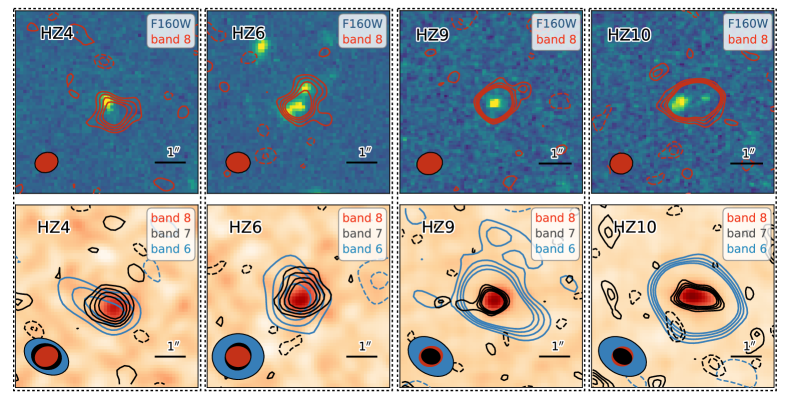
Figure 1: $6\arcsec\times 6\arcsec$ cutouts of our four sources. North is up and east is to the left. Top Panels: HST F160W (rest-frame $\sim 2500\,\mathring{\rm A}$) cutouts with ALMA Band 8 continuum contours (red). Bottom Panels: ALMA Band 8 continuum (background image) with contours showing Band 7 (black) and Band 6 (blue) continuum data from the literature. The solid contours start from 2$\,\sigma$ and end at $5\,\sigma$, and dashed contours indicate $-3\,\sigma$ and $-2\,\sigma$. The ALMA synthesised beams are shown for the different bands. All galaxies are significantly ($5-25\sigma$) detected in the far-IR continuum, and their flux peak positions are consistent each other within the beam sizes. There is a potential offset of the positions between the HST image and the far-IR detection for HZ4.

Table 2: Summary of Flux Measurements.

ID	z	$\lambda_{\rm band6}$	$f_{\rm{band6}}$	$\lambda_{\rm band7}$	$f_{\rm{band7}}$	$\lambda_{\rm band8}$	$f_{\rm{band8}}$
		$\left[\rm{\mu m}\right]$	$\rm{\left[\mu Jy\right]}$	$\left[\rm{\mu m}\right]$	$\rm{\left[\mu Jy\right]}$	$\left[\rm{\mu m}\right]$	$\rm{\left[\mu Jy\right]}$
HZ4	5.544	1294	$102\pm 26\,(\pm 6)$	1014	$189\pm 30\,(\pm 9)$	738	$524\pm 88\,(\pm 31)$
HZ6	5.293	1328	$256\pm 55\,(\pm 23)$	975	$404\pm 61\,(\pm 18)$	738	$610\pm 86\,(\pm 37)$
HZ9	5.541	1294	$274\pm 22\,(\pm 18)$	1008	$570\pm 67\,(\pm 29)$	738	$1109\pm 84\,(\pm 67)$
HZ10	5.657	1318	$706\pm 25\,(\pm 35)$	1027	$1519\pm 74\,(\pm 76)$	738	$2813\pm 129\,(\pm 169)$

• Notes: Flux errors in the parentheses are calibration error estimated in §2.3.

2 Data

We focus on four main-sequence galaxies to which we refer to as HZ4 ($z=5.544$), HZ6 ($z=5.293$), HZ9 ($z=5.541$), and HZ10 ($z=5.657$) in the following. These galaxies have been previously discussed by Riechers et al. (2014) and Capak et al. (2015) and are initially spectroscopically selected via Ly$\alpha$ and UV absorption lines from a large spectroscopic campaign with Keck/DEIMOS (Hasinger et al., 2018) on the Cosmic Evolution Survey (COSMOS, Scoville et al., 2007) field. All galaxies have been observed with different ALMA programmes covering their rest-frame wavelengths from $100\,{\rm\mu m}$ to $200\,{\rm\mu m}$ (see Table 1).

2.1 New ALMA Band 8 Observation

All four galaxies have been observed recently as part of the ALMA programme #2018.1.00348.S (PI: Faisst) at a frequency of $406.4\,{\rm GHz}$ (Band 8). This frequency was chosen to optimise the constraints on the infrared SED and to minimise the integration time to reach a S/N of $10$. At that frequency, the Band 8 atmospheric transmission is maximised and going to higher frequencies would increase the integration times significantly. On the other hand, Band 7 observes too low frequencies for robust constraints on the infrared SED together with the archival ALMA observations (see Appendix in Faisst et al., 2017). In the rest-frame of HZ4, HZ6, HZ9, and HZ10, Band 8 corresponds to wavelengths of $112.8\,{\rm\mu m}$, $117.3\,{\rm\mu m}$, $112.9\,{\rm\mu m}$, and $111.0\,{\rm\mu m}$, respectively. The observations were carried out in Cycle 6 between January 9 and 12, 2019 in the C43-2 compact configuration (maximal baseline $\sim 300\,{\rm m}$) at an angular resolution of $0.55\arcsec$ to $0.62\arcsec$ under good weather conditions (precipitable water vapor column between $0.38\,{\rm mm}$ and $0.87\,{\rm mm}$). The on-source exposure times for the galaxies were estimated from their $150\,{\rm\mu m}$ continuum luminosities and total to $1.48\,{\rm h}$, $2.24\,{\rm h}$, $0.64\,{\rm h}$, and $0.41\,{\rm h}$. For each target, the correlator was set up in dual polarisation to cover two spectral windows of $1.875\,{\rm GHz}$ bandwidth each at a resolution of $31.25\,{\rm MHz}$ ($\sim 23\,{\rm km\,s^{-1}}$) in each sideband and centered at $406.4\,{\rm GHz}$.

The Common Astronomy Software Application (CASA) version 5.4.0 was used for data calibration and analysis. For the data calibration, we used the scripts released by the QA2 analyst (ScriptForPI.py). We then produced continuum maps using the CASA task TCLEAN using multi-frequency synthesis (MFS) mode with NATURAL weighting scheme to maximise their sensitivities. During the TCLEAN process, we deconvolved synthesised beam down to $3\,\sigma$, where $\sigma$ is the background RMS of the image without beam deconvolution (i.e. “dirty image"). The resulting continuum sensitivities of the Band 8 maps are $34\,\rm{\mu Jy\,beam^{-1}}$, $40\,\rm{\mu Jy\,beam^{-1}}$, $57\,\rm{\mu Jy\,beam^{-1}}$, and $66\,\rm{\mu Jy\,beam^{-1}}$ for HZ4, HZ6, HZ9, and HZ10 respectively. All sources are significantly detected ($\rm{S/N}\simeq 8-25$) as expected from our observing strategy (top panels, Figure 1).

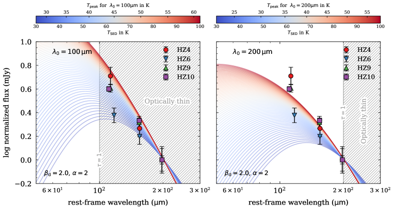
Figure 2: Infrared SED models assuming $\lambda_{0}=100\,{\rm\mu m}$ (left) and $\lambda_{0}=200\,{\rm\mu m}$ (right) and fixed $\alpha=2$ and $\beta_{\rm d}=2$ for different SED temperatures from $30\,{\rm K}$ (blue) to $100\,{\rm K}$ (red). The colour bar also indicated the dust peak temperature. The continuum fluxes of all galaxies except HZ6 can only be reproduced in the optical thin emission redward of $100\,{\rm\mu m}$ ($\lambda_{0}=100\,{\rm\mu m}$). This suggests optical thin dust emission. The observations are normalised to Band 6 (at $205\,{\rm\mu m}$).

2.2 Ancillary ALMA data

To measure continuum at longer wavelengths, we complemented our Band 8 observations with ancillary data available in the ALMA archive. All four sources were observed by several observing projects both in Band 6 and in Band 7. We refer interested readers to the papers listed below for more detail.

The rest-frame $\sim 200\,\rm{\mu m}$ (Band 6) observations are available from the ALMA project code 2015.1.00388.S (PI: N. Lu, Lu et al., 2018) and 2015.1.00928.S (PI: Pavesi, Pavesi et al., 2019) and the rest-frame $\sim 150\,\rm{\mu m}$ (Band 7) observations are available from the ALMA project code 2017.1.00428.L (ALPINE; PI: O. Le Fèvre, Le Fèvre et al., 2019; Bethermin et al., 2020; Faisst et al., 2020) for HZ4 and for HZ6, and 2012.1.00523.S (PI: P. Capak, Capak et al., 2015) for HZ9 and for HZ10. After we obtained data from the ALMA archive, we calibrated all data using the scripts released by the QA2 analyst (ScriptForPI.py). We use the appropriate versions of CASA as specified by the scripts.

To create continuum maps, we excluded channels closer than $\pm 3\sigma$ width of the [N ii] ($205\,\rm{\mu m}$) or [C ii] ($158\,\rm{\mu m}$) emission lines from the calibrated data. The emission line frequencies and widths are taken from previous studies (Capak et al., 2015; Pavesi et al., 2018a; Bethermin et al., 2020). After masking emission lines, we create continuum maps following the same procedure as for the Band 8 data using CASA task TCLEAN with NATURAL weighting scheme (see §2.1). The resulting sensitivities and synthesised beam resolutions are summarised in Table 1. All maps show significant ($\rm{S/N}\simeq 5-30$) continuum detections, with spatial positions that are consistent across different frequencies given the beam uncertainties (bottom panels, Figure 1).

2.3 Flux Calibration Errors

Given the significant detections and high flux densities measured for some of our sources, flux calibration errors are potentially a significant contributor to the overall uncertainties. We thus estimated the variability of all our flux calibrators. In particular, when flux calibrations are performed using secondary flux calibrators (i.e. quasars), we obtained the flux monitoring results from the ALMA calibrator source catalog both for Band 3 and for Band 7. We then estimated expected flux densities and errors in each observed frequency. The differences from the expected fluxes from each successive monitoring are used to estimate flux variabilities of observed frequencies. In doing so, we accounted for the typical measurement uncertainties of the expected flux densities. When flux calibrations are based on primary flux calibrators (i.e. solar systems objects), the flux calibrations are much less affected by the flux variabilities. Nevertheless, we applied conservative flux calibration errors of $5\,\%$ to take into account the potential modeling uncertainty of resolved flux calibrator observations. We estimated flux calibration errors of $6\,\%$ to $\sim 9\,\%$ for our observations (see Table 1).

Table 3: Summary of quantities derived from the infrared SED. All values (except $\beta_{\rm d}$) are computed by marginalising over $\beta_{\rm d}$. The quoted errors include all uncertainties and are $1\sigma$.

ID	$\beta_{\rm d}$	$T_{\rm SED}$	$T_{\rm peak}$	$\log{(L_{\rm IR})}^{a}$	$\log{(L_{\rm FIR})}^{b}$	$\log{(M_{\rm ISM})}$	$f_{\rm ISM}$	$\log({\rm SFR_{tot}})$	$t_{\rm depl}$
		$\left[\rm{K}\right]$	$\left[\rm{K}\right]$	$\left[\rm{L_{\odot}}\right]$	$\left[\rm{L_{\odot}}\right]$	$\left[\rm{M_{\odot}}\right]$		$\left[{\rm M_{\odot}\,yr^{-1}}\right]$	$\left[\rm{Myrs}\right]$
HZ4	2.01${}^{+0.69}_{-0.57}$	57.3${}^{+67.1}_{-16.6}$	42.4${}^{+28.7}_{-8.2}$	11.91${}^{+0.37}_{-0.91}$	11.83${}^{+0.44}_{-0.23}$	9.92${}^{+0.43}_{-0.50}$	0.67${}^{+0.21}_{-0.31}$	1.89${}^{+0.37}_{-0.91}$	97${}^{+265}_{-70}$
HZ6	1.60${}^{+0.58}_{-0.57}$	40.8${}^{+17.8}_{-7.2}$	33.9${}^{+9.9}_{-5.9}$	11.73${}^{+0.22}_{-0.34}$	11.52${}^{+0.24}_{-0.31}$	10.55${}^{+0.43}_{-0.45}$	0.73${}^{+0.17}_{-0.26}$	1.72${}^{+0.22}_{-0.34}$	755${}^{+2041}_{-544}$
HZ6†	1.85${}^{+0.69}_{-0.82}$	48.4${}^{+30.2}_{-10.8}$	30.8${}^{+15.4}_{-6.5}$	11.69${}^{+0.26}_{-0.51}$	11.50${}^{+0.29}_{-0.43}$	9.99${}^{+0.78}_{-0.62}$	0.37${}^{+0.49}_{-0.30}$	1.68${}^{+0.26}_{-0.51}$	212${}^{+173}_{-1094}$
HZ9	2.01${}^{+0.52}_{-0.70}$	49.4${}^{+29.0}_{-10.7}$	38.9${}^{+13.7}_{-5.8}$	12.14${}^{+0.21}_{-0.45}$	11.94${}^{+0.21}_{-0.33}$	10.39${}^{+0.44}_{-0.35}$	0.81${}^{+0.13}_{-0.19}$	2.13${}^{+0.21}_{-0.45}$	210${}^{+431}_{-141}$
HZ10	2.15${}^{+0.41}_{-0.54}$	46.2${}^{+16.2}_{-8.5}$	37.4${}^{+8.0}_{-4.9}$	12.49${}^{+0.15}_{-0.25}$	12.28${}^{+0.15}_{-0.21}$	10.72${}^{+0.36}_{-0.26}$	0.70${}^{+0.17}_{-0.16}$	2.48${}^{+0.15}_{-0.25}$	191${}^{+260}_{-107}$

• ^a Total infrared luminosity computed in the range from $3\,{\rm\mu m}$ to $1100\,{\rm\mu m}$.

• ^b Total far-IR luminosity computed in the range from $42.5\,{\rm\mu m}$ to $122.5\,{\rm\mu m}$.

• ^† Measurement with $\lambda_{0}=200\,{\rm\mu m}$, see text for more details.

3 Measurements

3.1 Continuum Flux Measurements

After we confirmed individual detections in all images, we performed continuum flux density measurements in the visibility domain. While imaged maps are useful to examine the achieved sensitivities and to validate source detections, map reconstructions depend on observational and imaging parameters such as the resolution and parameters used during the deconvolution processes. The visibility domain is less affected by these parameters.

We performed visibility-based flux measurements using the task UV_FIT from the software package GILDAS after creating continuum visibilities by masking emission lines, if present, following the same procedure as in §2.2. We used a single 2D Gaussian for visibility fitting, keeping source positions, source sizes, and integrated flux densities as free parameters. The resulting measurements for all of our sources are listed in the Table 2.

3.2 Infrared SED Fits and Dust Temperature

We use the Markov Chain Monte Carlo (MCMC) method provided by the Python package PyMC3 to fit the infrared SEDs of our four galaxies including all the three ALMA continuum measurements described above (Table 2). The SED is parameterised as the sum of a single modified black body and a mid-infrared power-law as described in Casey (2012) (see also Blain et al., 2003),

$$S(\lambda)=N_{\rm bb}\,f(\lambda;\beta_{\rm d},T_{\rm SED})+N_{\rm pl}\,\lambda^{\alpha}\,e^{-(\lambda/\lambda_{\rm c})^{2}}$$ (1)

with

$$N_{\rm pl}\equiv N_{\rm bb}\,f(\lambda_{\rm c};\beta_{\rm d},T_{\rm SED})$$ (2)

and

$$f(\lambda;\beta_{\rm d},T_{\rm SED})\equiv\frac{\left(1-e^{-(\lambda_{0}/\lambda)^{\beta_{\rm d}}}\right)\left(\frac{c}{\lambda}\right)^{3}}{e^{(h\,c)/(\lambda\,k\,T_{\rm SED})}-1}.$$ (3)

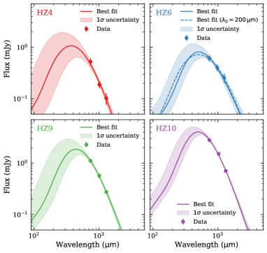
Figure 3: Best-fit infrared SEDs for the four galaxies derived from Equations 1 to 3 ($1\sigma$ uncertainty indicated by coloured band). The wavelength is given in observer frame. The dashed line shows the case with $\lambda_{0}=200\,{\rm\mu m}$ for HZ6. The new Band 8 continuum measurements ($110\,{\rm\mu m}$ rest-frame, $740\,{\rm\mu m}$ observed) probe better the peak of the infrared SED, which allows us to put the first constraints on the dust temperature and total infrared luminosity at these redshifts. Note that the scale of the $y-$axis is the same in all panels to show the differences in total flux.

In addition, the power-law turnover wavelength $\lambda_{\rm c}$ is dependent on $\alpha$ and $T_{\rm SED}$ (see Casey, 2012). Free parameters are $N_{\rm bb}$ (normalisation), $\alpha$ (slope of the mid-infrared power-law), $\beta_{\rm d}$ (emissivity index), $T_{\rm SED}$ (SED dust temperature), and $\lambda_{0}$ (wavelength where the optical depth is unity). Since our data do not constrain the SED blueward of rest-frame $\sim 110\,{\rm\mu m}$ (Band 8), we fix the mid-IR power-law slope to $\alpha=2.0$ as suggested by the measurements in Casey (2012).

The SED dust temperature (defined by Equation 1) should not be confused with the peak dust temperature, which is proportional to the inverse wavelength at the peak of the infrared emission via Wien’s displacement law,

$$T_{\rm peak}\,{\rm[K]}=\frac{2.898\times 10^{3}\,{\rm[\mu m\,K]}}{\lambda_{\rm peak}\,{\rm[\mu m]}}.$$ (4)

The SED and peak temperature can be considerably different as shown in Casey (2012). Note that both are a measure of the light-weighted dust temperature. This is in contrast to the cold dust emitted at $25\,{\rm K}$ in the Rayleigh-Jeans tail of the far-IR spectrum ($\gtrsim~{}250\,{\rm\mu m}$ rest-frame). This mass-weighted temperature is expected to be largely independent of redshift and other galaxy properties (see, e.g., Scoville et al., 2016; Liang et al., 2019).

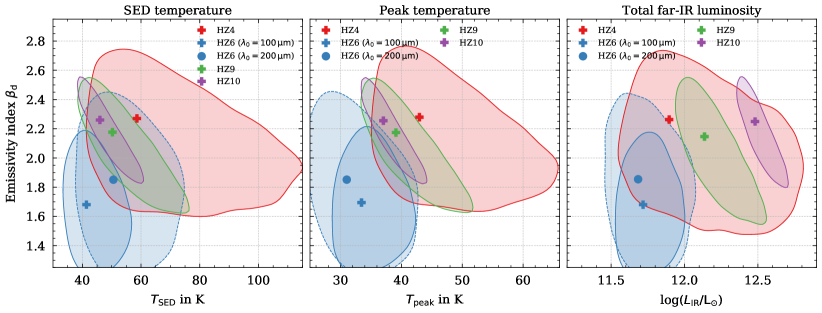
Figure 4: MCMC-derived $1\sigma$ contours of the SED (left) and peak (middle) dust temperature as well as the total ($3-1100\,{\rm\mu m}$) infrared luminosity (right) as a function of the emissivity index $\beta_{\rm d}$. The dashed contour shows the results for HZ6 in the optically thick case ($\lambda_{0}=200\,{\rm\mu m}$). Band 8 probes the wavelength close to the far-IR peak for our galaxies, hence allows us to put first constraints on dust temperatures at these redshifts.

A largely unknown fitting parameter is $\lambda_{0}$, the wavelength at which the optical depth $\tau$ equals unity (i.e., optically thick at bluer wavelengths). Based on observational studies at lower redshift, it is generally assumed that $\lambda_{0}\sim 200\,{\rm\mu m}$ (e.g., Blain et al., 2003; Conley et al., 2011; Rangwala et al., 2011; Casey, 2012; Riechers et al., 2013). However, as shown in Figure 2, our new Band 8 observations cannot be fit with $\lambda_{0}=200\,{\rm\mu m}$ for three out of four galaxies. Specifically, the two panels show rest-frame modified black body models (Equations 1 to 3 with fixed $\alpha=2$ and $\beta_{\rm d}=2$) for $\lambda_{0}=100\,{\rm\mu m}$ (left) and $\lambda_{0}=200\,{\rm\mu m}$ (right) for a range of SED temperatures (coloured from blue to red). The observed fluxes of our galaxies normalised to Band 6 (at $205\,{\rm\mu m}$) are shown by symbols. Clearly, our Band 8 observations (at rest-frame $110\,{\rm\mu m}$) cannot be explained with $\lambda_{0}=200\,{\rm\mu m}$ at any reasonable temperature for all of our galaxies except HZ6. The emission at $\sim 100\,\mu m$ is therefore likely optically thin and we therefore assume $\lambda_{0}=100\,{\rm\mu m}$ in the following. This is consistent with theoretical models for low-opacity dust (Draine, 2006; Scoville & Kwan, 1976). Different values of $\alpha$ and $\beta_{\rm d}$ in a reasonable range do not change this conclusion.

The observations of HZ6 can be reconciled with optically thick emission up to rest-frame $200\,{\rm\mu m}$. As found in Capak et al. (2011), HZ6 is part of a protocluster at $z=5.3$. Specifically, HZ6 consists of three components separated by $\Delta v<50\,{\rm km\,s^{-1}}$ in radial velocity and $<3\,{\rm kpc}$ in projected distance (Figure 1). The components are likely gravitationally interacting and a past close passage is suggested by the diffuse rest-frame UV emission and a ‘crossing time’ of $\sim 50\,{\rm Myrs}$. The latter is estimated using $t_{\rm cross}\simeq(G\,\bar{\rho})^{-\frac{1}{2}}$, where $\bar{\rho}$ is the average mass density and $G$ the gravitational constant, with values based on observations ($r=3\,{\rm kpc}$ and total enclosed mass of $10^{10}\,{\rm M_{\odot}}$ for a single component). This setup could cause a more optically thick medium by, e.g., the compression of gas and/or the formation of dust. With the current data, it is not possible to make further conclusions and we therefore show in the following derivations using both values of $\lambda_{0}$ for HZ6.

For the MCMC fit to the infrared SEDs of our galaxies, we adopt a flat prior for the dust temperature, and a Gaussian prior for $\beta_{\rm d}$ with a $\sigma(\beta_{\rm d})=0.5$ centered on $1.8$ (see, e.g., Hildebrand, 1983). The normalisation is also sampled with a Gaussian prior in linear space around an initial guess derived by the normalisation in Band 7. We found that fitting in linear space is more appropriate given the errors of the data. To perform the fitting, we use the No-U-Turn Sampler (NUTS, Hoffman & Gelman, 2011), which is an extension to the Hamilton Monte Carlo algorithm (Neal, 2012) and is less sensitive to tuning. We draw $18\,000$ samples in total with a target acceptance of $0.99$, which we found to provide the best performance.

Figure 3 shows the best-fit infrared SEDs together with the $1\sigma$ uncertainties for each of our galaxies. Thanks to our Band 8 data at rest-frame wavelengths of $110\,{\rm\mu m}$, we can put more stringent constraints on the location of the peak of the infrared SED. The galaxies HZ4 and HZ6 are fainter, resulting in larger uncertainties of the fit. While the mid-IR blueward of the peak is poorly constrained, the RJ tail (at $>1000\,{\rm\mu m}$ observed frame) can be robustly extrapolated based on our data.

Figure 4 shows the derived SED (left) and peak (middle) dust temperature as well as total infrared luminosity (right) contours ($1\sigma$) as a function of the emissivity index $\beta_{\rm d}$ for our four galaxies. We find emissivity indices between $1.6$ and $2.4$ for all galaxies, with a median of $2.0$, which is consistent with measurements at lower redshifts (e.g., Casey, 2012; Conley et al., 2011). The dust SED temperatures range between $40-60\,{\rm K}$ with a median at $48\,{\rm K}$. For the dust peak temperatures, we find a range of $30-43\,{\rm K}$ with a median of $38\,{\rm K}$. The total infrared luminosities ($L_{{\rm IR}}$) are derived by integrating the best-fit SED between $3-1100\,{\rm\mu m}$ and range between $5-30\times 10^{11}\,{\rm L_{\odot}}$. We note that the peak temperature and the total infrared luminosity is insensitive to the assumed $\lambda_{0}$. We also quote far-IR luminosities ($L_{{\rm FIR}}$) measured by integrating the flux between $42.5\,{\rm\mu m}$ and $122.5\,{\rm\mu m}$ for easier comparison with the literature. All measurements are summarised in Table 3.

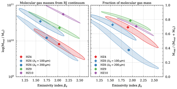
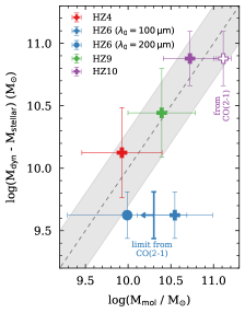
Figure 5: MCMC-derived $1\sigma$ contours of the molecular gas masses (left) and fractions (middle) as a function of the emissivity index $\beta_{\rm d}$. The molecular gas masses have been estimated using the RJ dust continuum at rest-frame $850\,{\rm\mu m}$ using the method by Scoville et al. (2016). The three ALMA continuum frequencies put the first robust constraints on the emissivity index (far-IR slope) at these high redshifts, which is critical to derive molecular gas masses. The right panel shows the comparison of our dust-continuum derived molecular gas masses and the difference between dynamical and stellar mass (expected to be equal to the total gas mass modulo dark matter). Note that HZ6 (blue) has a complicated velocity structure due to its major merger nature, which makes the measurement of its dynamical mass significantly uncertain. The molecular gas mass measurements obtained from the CO($2-1$) transition (Pavesi et al., 2019) are also shown for comparison. They largely agree with our measurements.

3.3 Molecular Gas Masses from the RJ dust continuum

The measurement of molecular gas masses of galaxies is crucial to understand the star formation processes determining their growth and evolution. Low-$J$ transitions of the CO molecule are used regularly at $z<2$ (e.g., Tacconi et al., 2010; Genzel et al., 2015; Freundlich et al., 2019), but this is not feasible for large samples of normal galaxies at higher redshifts due to the large amount of necessary telescope time. Currently only very few observations of CO in normal galaxies at $z>5$ exist (D’Odorico et al., 2018; Pavesi et al., 2019). Alternatively, the far-IR [C ii] emission line can be used as tracer of molecular gas (De Looze et al., 2014; Zanella et al., 2018; Dessauges et al., submitted,, 2020), however, there are considerable uncertainties in its use due to the unknown origin of C⁺ emission.

Alternatively, molecular gas masses can be measured using the dust continuum emission emitted at rest-frame $850\,{\rm\mu m}$ in the RJ tail of the far-IR spectrum (Scoville et al., 2014, 2016, 2017; Hughes et al., 2017; Kaasinen et al., 2019; Dessauges et al., submitted,, 2020). For current samples of main-sequence galaxies at high redshifts, the far-IR slope (defined by the emissivity index $\beta_{\rm d}$) cannot be constrained directly due to the lack of observations. Significant assumptions have therefore to be made to quantify the rest-frame $850\,{\rm\mu m}$ continuum. With our 3-band data sampling the SED redward of the far-IR peak, we can constrain the far-IR slope for the first time at these redshifts directly. The molecular gas masses are then derived using the observed flux at rest-frame $205\,{\rm\mu m}$ (Band 6, $S_{\rm\nu_{obs}}$ in mJy) that is extrapolated to $805\,{\rm\mu m}$ using the full probability distribution of $\beta_{\rm d}$ from our MCMC fit and equation (16) in Scoville et al. (2016) with similar assumptions,

$$M_{\rm mol} =1.78\,S_{\rm\nu_{obs}}\,(1+z)^{-(3+\beta_{\rm d})}\,\left(\frac{\nu_{\rm 850\mu m}}{\nu_{\rm obs}}\right)^{2+\beta_{\rm d}}\,D_{\rm L}^{2}(z)$$

$$\times\left(\frac{6.7\times 10^{19}}{\alpha_{850}}\right)\,\left(\frac{\Gamma_{\rm RJ,z=0}}{\Gamma_{\rm RJ}}\right)\times 10^{10}\,{\rm M_{\odot}}.$$

In this case, $D_{\rm L}(z)$ is the luminosity distance at redshift $z$ in Gpc and we assume $\alpha_{850}=6.7\times 10^{19}\,{\rm erg\,s^{-1}\,Hz^{-1}\,M_{\odot}^{-1}}$, which is the average measured for galaxies at $z<3$ (Scoville et al., 2016). $\Gamma_{\rm RJ}(\nu_{\rm obs},T_{d},z)$ is the correction for departure in the rest-frame of the Planck function from Rayleigh-Jeans and depends on the mass-weighted dust temperature (different from $T_{\rm SED}$ or $T_{\rm peak}$, which are luminosity-weighted temperatures). For the latter, we adopt $25\,{\rm K}$, but assuming higher temperatures such as $35\,{\rm K}$ lowers the inferred molecular masses by less than $10\%$.

The left panel of Figure 5 shows the derived $1\sigma$ contours of the molecular masses for our galaxies from our MCMC fit. The masses range between $0.3-8.0\times 10^{10}\,{\rm M_{\odot}}$. The middle panel shows the molecular gas fractions ($f_{\rm gas}=M_{\rm mol}/(M_{\rm mol}+M_{\rm stellar})$, using stellar masses from Capak et al. (2015)), which range between $30\%$ and $80\%$. Statistically, this is consistent with the ALPINE sample at $z=5.5$ (Dessauges et al., submitted,, 2020). This is expected as our galaxies are consistent with the average masses and SFRs of the ALPINE sample (see Faisst et al., 2020). The right panel of Figure 5 compares the dust continuum gas masses with the difference between dynamical and stellar masses. This difference should yield total gas masses modulo the contribution of dark matter, which is expected to be on the order of $10-20\%$ or less at the radii probed here (Barnabè et al., 2012). The dynamical masses are derived inside a half-light radius from the [C ii] emission line velocity profile (Pavesi et al., 2019). Generally, we find an agreement within a factor of two ($<1\sigma$) between gas masses derived from dust continuum and dynamical masses. However, assuming $\lambda_{0}=100\,{\rm\mu m}$ for the fit of HZ6 results in a $2\sigma$ discrepancy. As noted earlier, HZ6 is a three-component major merger system with significant gravitational interaction. The complex velocity structure likely causes large uncertainties in its dynamical mass estimate. In addition, the $850\,{\rm\mu m}$-continuum derived gas mass encompasses the whole extended system, while the dynamical mass captures only a fraction of the gas. Both can explain its larger offset from the 1-to-1 line compared to the other galaxies. On the other hand, if the dynamical mass is reliable, this indicates once more that the emission in HZ6 could be optically think up to $200\,{\rm\mu m}$ (as $\lambda_{0}=200\,{\rm\mu m}$ results in discrepancy).

Pavesi et al. (2019) report a gas mass estimate from CO($2-1$) emission for HZ6 and HZ10, assuming a Milky Way-like CO to molecular gas conversion factor ($\alpha_{\rm CO}=4.5\,{\rm M_{\odot}/(K\,km\,s^{-1}\,pc^{2})}$) and brightness temperature ratio $R_{21}=1$. They find $1.3\times 10^{11}\,{\rm M_{\odot}}$ for HZ10 and a limit $<2\times 10^{10}\,{\rm M_{\odot}}$ for HZ6 (see Figure 5). The CO-gas mass estimate of HZ10 is a factor $2.5$ larger ($\sim 1\sigma$ discrepancy) than what we measure from dust continuum and dynamical masses. The upper limit in CO-derived gas mass for HZ6 is consistent with our measurement if assuming $\lambda_{0}=200\,{\rm\mu m}$ (but not if optically thin dust at $100\,{\rm\mu m}$). The discrepancy of the measurements for HZ10 are not significant, given the large measurement errors as well as uncertainties in $\alpha_{\rm CO}$ and the brightness temperature ratio. However, large $\alpha_{\rm CO}$ values above $20$ that are expected for metal-poor environments such as in the Small Magellanic Cloud (see Leroy et al., 2011) can be excluded for HZ10. This is in agreement with earlier studies that suggest that HZ10 is fairly metal enriched, even close to solar metallicity, based on its strong rest-frame UV absorption lines (e.g., Faisst et al., 2017; Pavesi et al., 2019). Clearly, larger samples or more precise measurements have to be obtained in order to draw final conclusions.

From the total infrared luminosity we can derive the total SFRs using the Kennicutt (1998) relation and from that the gas depletion time via $t_{\rm depl}=\rm M_{\rm mol}$/SFR_IR. For HZ4, HZ9, and HZ10 find values between $100-220\,{\rm Myrs}$. This is in agreement with the trend of decreasing depletion time with higher redshifts (e.g., Scoville et al., 2016). For HZ6, the depletion time depends on the assumed $\lambda_{0}$. For $\lambda_{0}$ equal to $100\,{\rm\mu m}$ and $200\,{\rm\mu m}$ we derive a depletion time of $755\,{\rm Myrs}$ and $212\,{\rm Myrs}$, respectively.

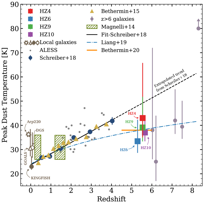
Figure 6: Peak dust temperature ($T_{\rm peak}$) evolution with redshift. The large coloured squares show our galaxies at $z\sim 5.5$. We also show galaxy samples at $z=0$ from the KINGFISH (dark gray circle), DGS (dark gray open circle), and GOALS (dark gray open triangle) samples (shifted by $0.02$ in redshift for clarity), and galaxies at $z=0.2-4.0$ (matched to our luminosity range) from ALESS (gray small circles, Smail & Walter, 2014; Schreiber et al., 2018), Béthermin et al. (yellow triangles, 2015), and Magnelli et al. (hatched rectangles, 2014), as well as $z>6$ (light purple circles, Knudsen et al., 2016; Hashimoto et al., 2019; Bakx et al., 2020). The data for Arp220 is taken from Rangwala et al. (2011). For consistency, we re-measured the $T_{\rm peak}$ of the local galaxies as well as $z>6$ galaxies with our method (see Section 3). The latter include CMB correction. The fit to the Schreiber et al. (2018) data is shown in black (dashed when extrapolation), together with the expectation from hydrodynamic simulations (blue dot-dashed, Liang et al., 2019; Ma et al., 2019), and the temperature derived from an average template for ALPINE galaxies (orange line, Bethermin et al., 2020). Galaxies at $z>4$ have warmer peak temperatures compared to average local galaxies, however, are $5-10\,{\rm K}$ cooler than what would be predicted from the trend found at $z<4$. This indicates a flattening of the $T_{\rm peak}-z$ relation at $z>4$, which could be due to a lower dust abundance or opacity in high redshift galaxies.

4 Discussion

4.1 Rising Temperature towards High Redshifts?

Figure 6 puts our measurements at $z\sim 5.5$ into context with measurements from the literature at $z<4$ and $z>6$. At $z=0$, we show peak temperature measurements derived in Faisst et al. (2017, using Equations 1 to 3) for the KINGFISH sample (Skibba et al., 2011), the Dwarf Galaxy Sample (DGS, Madden et al., 2013), and the GOALS sample (Kennicutt et al., 2011). The data for Arp220 is taken from Rangwala et al. (2011). At $z=0.2-4.0$ from the ALMA LABOCA ECDFS Sub-mm Survey (ALESS, Smail & Walter, 2014; Schreiber et al., 2018), the sample from Béthermin et al. (2015), and galaxies at from Magnelli et al. (2014). For the latter, we select a similar range in total infrared luminosity as our sample ($\log(L_{{\rm IR}}/{\rm L_{\odot}})\sim 10.5-12.5$). We also note that the stellar mass range is similar to our sample. At $z>6$ we show galaxies from Bakx et al. (2020, lower limit), Knudsen et al. (2016), and Hashimoto et al. (2019). For the latter two, we have re-measured the peak temperature with our method. The trend derived from hydrodynamic simulations (Liang et al., 2019; Ma et al., 2019) is shown as dot-dashed line.

Our measurements at $z\sim 5.5$ show elevated dust temperatures compared to average local galaxies such as from the KINGFISH sample. Taking the uncertainties into account, we can exclude peak temperatures of less than $30\,{\rm K}$. The median peak temperature measured for our galaxies is at $38\pm 5\,{\rm K}$, with a low-probability tail towards higher temperatures (Figure 4). However, although the temperatures at $z\sim 5.5$ are higher compared to average local galaxies, we find that our values are about $10\,{\rm K}$ below what would be predicted from an extrapolation of observational data at $z<4$. Particularly, the Schreiber et al. (2018) infrared SED template at $z=4$ suggests a peak temperature of $42\,{\rm K}$. If extrapolated to $z=5.5$, this results in $\sim 46\,{\rm K}$, which is $\sim 5-10\,{\rm K}$ higher than what we measure from our data (at similar infrared luminosity). On the other hand, our measurements are consistent with the empirically derived infrared SED of $4<z<6$ galaxies from Bethermin et al. (2020), who find an average peak temperature of $38\,{\rm K}$. Furthermore, we find similar peak temperatures as reported at $z>6$ by the various studies.

Summarising, the peak temperatures of high-$z$ galaxies are warmer compared to average local galaxies, which has to be taken into account when parameterising the infrared SEDs of these galaxies. However, our observational data suggest that the peak temperature (i.e., the wavelength at peak emission of the infrared SED) does not evolve anymore strongly beyond redshifts $z=4$ for a fixed total infrared luminosity. This behaviour is reproduced in hydrodynamic simulations (e.g., Liang et al., 2019; Ma et al., 2019), which show a flattening of the temperature evolution with redshift for galaxies selected with $L_{{\rm IR}}>10^{11}\,{\rm L_{\odot}}$ (Figure 6).

4.2 Explaining the Observed $T_{\rm peak}(z)$ Evolution
with an Analytical Model of a Spherical Dust Cloud

In the previous section we have constrained the evolution of the peak temperature with redshift. Our unique observations at $z\sim 5.5$ and literature data at lower redshifts suggest that the temperature rises up to $z\sim 4$ and then tends to flatten off. At this point, we note that the increase in SED or peak temperature with redshift is merely a statement on a shift in the wavelengths at which the infrared SED peaks, i.e., its shape. This shift can be due to several physical reasons, including changes in the UV luminosity of a central source (i.e., the young stars), the dust mass density or the opacity of the dust. Such dependencies have been seen observationally in the local galaxy samples (Figure 6). For example, the KINGFISH sample (consisting of mostly solar metallicity and infrared fainter ($10^{10}-10^{11}\,{\rm L_{\odot}}$) galaxies) shows peak temperatures between $20\,{\rm K}$ and $30\,{\rm K}$. On the other hand, the IR luminous ($10^{11}-10^{12}\,{\rm L_{\odot}}$) GOALS sample (also close to solar metallicity) shows higher average peak temperatures ($25-40\,{\rm K}$). The DGS sample shows similarly high peak temperatures as the GOALS sample at less than a tenth solar metallicity and $L_{{\rm IR}}<10^{11}\,{\rm L_{\odot}}$. This suggests that $T_{\rm peak}$ correlates negative with metallicity and positive with $L_{{\rm IR}}$ (see figure 4 in Faisst et al., 2017). These physical relations can make selection effects (such as a survey limit in total infrared luminosity) mimic a temperature increase at $z<4$. However, as shown in table 1 of Schreiber et al. (2018), even at a fixed total infrared luminosity, the trend of increasing peak temperatures from $25\,{\rm K}$ to $40\,{\rm K}$ at $z=0.3-4.0$ persists.

In the following, we use a simple analytical model to investigate how the output of UV photons from a dust-enshrouded source (specifically the ratio between UV luminosity and dust mass) and the density of dust (i.e., the dust opacity) affect the shape of the infrared SED and with it the emergent peak temperature measured by an external observer.

We model the emitted heat (and hence peak temperature) from a dust cloud around stars using a model based on Scoville & Kwan (1976) that will be described in a forthcoming work (Scoville et al. in prep.). The model assumes a central source of UV light enshrouded in a dust cloud with spherical symmetry and constant density, and calculates the heating in concentric shells of dust mass. Secondary heating (from re-emitted light) is included, as well as the increased background temperature by CMB heating at high redshift. The latter, however, does not affect the dust temperature below $z=6$ significantly. In the following, we consider models for different intrinsic (i.e., obscured plus unobscured) UV luminosities and dust cloud radii. For the UV luminosity we choose $10^{11}$ and $10^{12}\,{\rm L_{\odot}}$, which is expected for our galaxies assuming that the intrinsic UV luminosity equals the total emitted infrared luminosity (energy conservation). For the radius we assume $2$ and $4\,{\rm kpc}$, consistent with the sizes of far-IR emission observed for our galaxies ($\sim 0.5\arcsec$ at $z=5.5$).

Figure 7 shows the peak temperature of the spectrum of emergent light computed for our different models as a function of dust mass. Note that dust mass in this case directly corresponds to dust density, hence opacity, as the radius of the cloud is fixed. This figure shows several trends. First, the change in peak temperature as a function of UV luminosity is apparent. Specifically, increasing the UV luminosity by an order of magnitude increases the temperature by a factor of $\sim 1.6$. This is expected because $T_{\rm peak}\propto L_{\rm UV}^{1/5}$ for emissivity varying as $\lambda^{-1}$ and optically thin dust at the far-IR peak. Second, for a given UV luminosity, the peak temperature increases for decreasing opacity (i.e., dust mass or density). This can be explained by the fact that hot dust at the peak of the infrared SED becomes visible to the observer as the opacity drops. At a certain value of opacity, the temperature ceases to rise. For a dust cloud radius of $2\,{\rm kpc}$ ($4\,{\rm kpc}$), this is reached at a dust mass of $10^{9}\,{\rm M_{\odot}}$ ($10^{10}\,{\rm M_{\odot}}$), which translates into an average dust mass density of $\bar{\rho}_{d}\sim 3\times 10^{7}\,{\rm M_{\odot}\,kpc^{-3}}$. Note that this number is independent of the intrinsic UV luminosity of the dust-enshrouded source.

Taking the output of this model at face value, the general increase of dust peak temperature with increasing redshift (at roughly fixed total infrared luminosity) can be explained by a decreasing dust opacity, which causes hot dust at short wavelengths to become optically thin and therefore visible to ALMA. In fact, several observations point in this direction. For example, the blue UV continuum slopes of galaxies in the early universe suggest that UV light is less attenuated by dust (e.g., Bouwens et al., 2014). At the same time, the fraction of dust-obscured star formation decreases significantly at $z>4$ (Fudamoto et al., 2020). The current lack of galaxies observed with very hot temperatures at $z>5$ (that would be expected by the trends found at $z<4$) can also be motivated by our model. As the dust opacity (i.e., dust mass density) continues do decrease at higher redshifts, the hot dust becomes optically thin and its temperature ceases to rise (Figure 2). In our model, this happens at an average dust mass density of $3\times 10^{7}\,{\rm M_{\odot}\,kpc^{-3}}$. This is indeed in similar to what is expected for our galaxies: Assuming an average molecular gas mass of $3\times 10^{10}\,{\rm M_{\odot}}$ (Section 3.3), a gas-to-dust ratio of $100$, and an average size of $2\,{\rm kpc}$, we estimate a dust mass density of $\sim 10^{7}\,{\rm M_{\odot}\,kpc^{-3}}$.

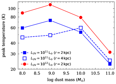
Figure 7: Dependence of peak temperature of emergent light on dust mass and central UV luminosity based on a symmetric shell model (Scoville et al. in prep.). The model assumes two different radii of the spherical dust cloud ($2$ and $4\,{\rm kpc}$) and two intrinsic UV luminosities ($10^{11}$ and $10^{12}\,{L_{\odot}}$) of the embedded source. Due to the fixed size of the dust cloud, the dust volume density and dust opacity increase to the right. The temperature drops at high dust masses (high opacity) because the hotter dust becomes optically thick. The temperature ceases to rise at a dust mass density of $3\times 10^{7}\,{\rm M_{\odot}\,kpc^{3}}$ independent of UV luminosity.

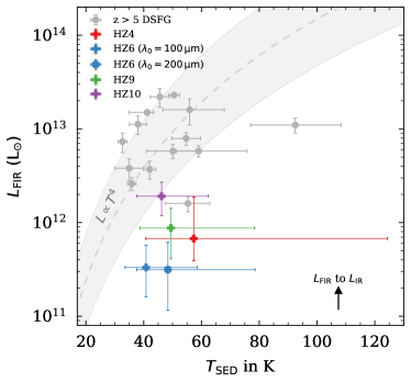
Figure 8: Comparison of SED temperature and far-IR luminosity ($L_{{\rm FIR}}$) to a sample of DSFGs at $z>5$ from Riechers et al. (2020). The luminosity is measured consistently between $42.5\,{\rm\mu m}$ and $122.5\,{\rm\mu m}$ (the arrow shows the difference to $L_{{\rm IR}}$). Our galaxies fall off the $L\propto T^{4}$ relation (here normalised median luminosity and temperature of the DSFGs with $0.5\,{\rm dex}$ range indicated). For a given luminosity, they are warmer than expected from this relation. This offset may be caused by different dust abundances, dust surface densities, or dust opacities between DSFGs and normal galaxies.

4.3 Comparison with Dusty Star-Forming Galaxies at $z>5$

In Figure 8, we compare the far-IR luminosity and SED temperatures of our galaxies to a compilation of infrared luminous dusty star-forming galaxies (DSFGs) at $z>5$ from Riechers et al. (2020) from the CO Luminosity Density at High Redshift survey (COLDz, Pavesi et al., 2018b; Riechers et al., 2019). For a fair comparison, we show SED dust temperatures and far-IR luminosities ($L_{{\rm FIR}}$). One would expect that for an increasing far-IR luminosity, the dust temperature increases (c.f. Figure 7). This is indicated by the $L\propto T^{4}$ relation (optically thick case) normalised to the median of the DSFGs,

$$L_{{\rm FIR}}=9.4\times 10^{12}\,\left(\frac{T_{\rm SED}}{50.1}\right)^{4}\,\,L_{\odot}.$$ (5)

However, our galaxies seem to be significantly warmer than predicted by this relation, or, for a given temperature their far-IR luminosity is too faint. Formulated in a different way, over 2.5 orders of magnitudes in infrared luminosity, the peak dust temperature is constant, which is in direct contradiction to what is found in the local universe (e.g., Magnelli et al., 2014). Since the galaxies are at similar redshifts, this indicates a fundamental difference in the dust properties of in the two samples. Capitalising on the previous sections and our analytical model, a higher dust abundance and/or dust surface density in the DSFGs would explain the observed differences. Furthermore, as mentioned above and in Faisst et al. (2017), metallicity (likely connected to dust opacity) has a strong impact on the SED and peak dust temperature. A lower metallicity in our galaxies compared to the DSFGs would increase their temperature at a fixed far-IR luminosity and push them off the $L\propto T^{4}$ relation.

4.4 A Final Note on Implication on $L_{{\rm IR}}$ Measurements

The evolution of the shape of the infrared SED with redshift has important consequences on the measurement of the total infrared luminosity. This quantity is important in several ways, for example, for the computation of dust masses and total star formation rates or the dust properties of high-redshift galaxies via the study of the IRX$-\beta$ relation. For surveys such as ALPINE, which target large numbers of main-sequence high-redshift galaxies, only one far-IR data point at $150\,{\rm\mu m}$ exists per galaxy. The above quantities therefore depend strongly on the assumed shape of the infrared SED ($\beta_{\rm d}$, $\alpha$, and temperature). Using the 3-band constraints on the infrared SEDs of our four galaxies, we can test previous measurements of the total infrared luminosity that are based on only the $150\,{\rm\mu m}$ continuum data point.

We derive total infrared luminosities between $\log(L_{{\rm IR}})=11.7-12.5$ for our galaxies (Table 3). Previously obtained luminosities by Capak et al. (2015), based on $150\,{\rm\mu m}$ continuum only, also assumed Equation 1, however, a lower temperature prior ($T_{\rm SED}=25-45\,{\rm K}$ or $T_{\rm peak}=20-30\,{\rm K}$) and $\lambda_{0}=200\,{\rm\mu m}$, but consistent emissivity range ($\beta_{\rm d}=1.2-2.0$). With these assumptions, $L_{{\rm IR}}$ would be underestimated consistently by $0.3-0.6\,{\rm dex}$ (factors $2-4$). In Bethermin et al. (2020), an average infrared SED created from stacked photometry of COSMOS galaxies between $4<z<6$ is normalised to the $150\,{\rm\mu m}$ data points of the ALPINE galaxies to derive their total luminosities. This approach leads to consistent total infrared luminosities with ours within less than $0.2\,{\rm{\rm dex}}$ ($<60\%$ difference). This result is also reflected in the good agreement of $T_{\rm peak}$ between their average infrared SED and our best fits (c.f., Figure 6). This comparison shows that (at least statistically) the total infrared luminosities of the ALPINE sample derived in Bethermin et al. (2020) are reasonable and highlights the importance of temperature assumptions in deriving this quantity.

5 Conclusions

We have acquired ALMA Band 8 data for four galaxies at $z\sim 5.5$ to put improved constraints on their infrared SEDs, specifically their peak dust temperatures, total infrared luminosities, and molecular gas masses. The continuum measurements at a rest-frame wavelength of $\sim 110\,{\rm\mu m}$ are blueward of other measurements from the literature in Band 6 ($\sim 200\,{\rm\mu m}$) and Band 7 ($\sim 150\,{\rm\mu m}$) and therefore extend the baseline towards the peak of infrared emission. The infrared SEDs are fit using a modified black body with mid-IR power law. The peak temperature is derived using Wien’s law and the molecular gas masses are measured using the extrapolated $850\,{\rm\mu m}$ continuum emission. The measurement of the latter benefits from our so far strongest constraints on the dust emissivity index $\beta_{\rm d}$ at these high redshifts. In the following, we summarise our findings:

• The best-fit peak temperatures range at $30-43\,{\rm K}$ (median of $38\,{\rm K}$, Figure 4). These temperatures are warmer compared to average local galaxies but $5-10\,{\rm K}$ lower than what would be predicted from trends at $z<4$ at similar infrared luminosities. Our measurements are consistent with the most recent hydrodynamical zoom-in simulations, as well as measurements at $z>6$.

• We find dust emissivity indices ($\beta_{d}$) between $1.6$ and $2.4$ with a median of $2.0$ (Figure 4) for our galaxies, consistent with measurements at lower redshifts.

• Our new Band 8 data suggest that the emission between rest-frame $100-200\,{\rm\mu m}$ is optically thin (i.e., can be fit with $\lambda_{0}~{}=~{}100\,{\rm\mu m}$) for three of our galaxies (Figure 2). An exception is HZ6, which is a gravitationally interacting three-component major merger and can be fit with optically thick emission below $200\,{\rm\mu m}$ ($\lambda_{0}=200\,{\rm\mu m}$).

• The molecular gas masses range between $10^{10}$ and $10^{11}\,{\rm M_{\odot}}$, corresponding to molecular gas fractions between $30\%$ and $80\%$ (Figure 5). They are in good agreement with the difference between dynamical and stellar masses. From this, we expect gas depletion time scales of $100-220\,{\rm Myrs}$ in good agreement with the expected decrease of depletion time with redshift. A comparison to gas masses derived from CO($2-1$) emission suggests an $\alpha_{\rm CO}$ conversion factor for HZ6 and HZ10 similar to our Milky Way (high values as measured in the SMC can be excluded).

At $z<4$, several studies find an increase in dust peak temperature at a roughly fixed total infrared luminosity. Our sample and measurements at $z>6$ do not suggest a further increase of temperature beyond $z=5$. The generally higher peak temperatures at $z=5.5$ compared to average local galaxies can be explained by the decreasing dust abundance (or density) at high redshifts. Specifically, as the dust opacity drops, hot dust becomes more optically thin and is visible to the external observer. The lack of dust temperature evolution at $z>5$ can be explained in similar terms. Our model shows that once the dust density falls below a certain value, the emergent peak temperature ceases to rise. Interestingly, this limit is on the same order of magnitude as the average dust mass density expected for our galaxies.

Compared to DSFGs at similar redshifts ($z>5$), our galaxies have warmer temperatures than what would be expected from their (factor of $10$) lower infrared luminosities. This difference could be explained by a larger dust abundance and/or higher metal content of DSFGs and is in agreement with our model predictions. Metallicity measurements with the James Webb Space Telescope for these two populations of galaxies will certainly help to identify what causes these differences.

One of the remaining interesting question is the connection between dust and gas. While a decrease of dust abundance or dust density may explain the observed $T_{\rm peak}-z$ evolution, at the same time the observed increase of the gas fraction (and hence dust abundance given a fixed gas-to-dust ratio) with redshift would argue for the opposite. An increasing gas-to-dust ratio with redshift due to a general decrease in metallicity (e.g., Leroy et al., 2011), could resolve this dilemma.

The number of ALMA observations at high redshifts is increasing rapidly as large surveys are becoming more frequent. Our Band 8 data are an important step to constrain better the infrared SEDs of post-reionisation galaxies. They can be used to inform and improve the assumptions that have to be made in order to measure important infrared SED based quantities as well as to test theoretical predictions. However, our conclusions are currently based on a sample of only four galaxies, which are, due to observing time constraints, among the infrared brightest galaxies at $z\sim 5.5$. Larger samples with similar measurements are crucial to advance our understanding. As shown by the comparison of gas masses derived by the dust-continuum and the CO($2-1$) emission, at least HZ6 and HZ10 have similar CO to ${\rm H_{2}}$ conversion factors to our Milky Way, which suggests metal enriched environments. This is also suggested by the deep absorption features of their rest-frame UV spectra. It is therefore likely that we are missing more metal poor systems, which could be the more common type of galaxies. Furthermore, our small sample also shows a diversity of galaxies (isolated galaxies, mergers, etc) that links to different dust properties, which should be explored. Our simple model can motivate certain trends seen in our sample, but to understand in depth the physics driving the observational results, similar observations for larger samples will be necessary in the future.

References

- Ando et al. (2007) Ando M., Ohta K., Iwata I., Akiyama M., Aoki K., Tamura N., 2007, PASJ, 59, 717
- Bakx et al. (2020) Bakx T. J. L. C., et al., 2020, MNRAS, 493, 4294
- Barnabè et al. (2012) Barnabè M., et al., 2012, MNRAS, 423, 1073
- Béthermin et al. (2015) Béthermin M., et al., 2015, A&A, 573, A113
- Bethermin et al. (2020) Bethermin M., et al., 2020, arXiv e-prints, p. arXiv:2002.00962
- Blain et al. (2003) Blain A. W., Barnard V. E., Chapman S. C., 2003, MNRAS, 338, 733
- Bouché et al. (2012) Bouché N., et al., 2012, MNRAS, 419, 2
- Bouwens et al. (2009) Bouwens R. J., et al., 2009, ApJ, 705, 936
- Bouwens et al. (2012) Bouwens R. J., et al., 2012, ApJ, 754, 83
- Bouwens et al. (2014) Bouwens R. J., et al., 2014, ApJ, 793, 115
- Capak et al. (2011) Capak P. L., et al., 2011, Nature, 470, 233
- Capak et al. (2015) Capak P. L., et al., 2015, Nature, 522, 455
- Casey (2012) Casey C. M., 2012, MNRAS, 425, 3094
- Chabrier (2003) Chabrier G., 2003, PASP, 115, 763
- Conley et al. (2011) Conley A., et al., 2011, ApJ, 732, L35
- D’Odorico et al. (2018) D’Odorico V., et al., 2018, ApJ, 863, L29
- Davidzon et al. (2017) Davidzon I., et al., 2017, A&A, 605, A70
- Davidzon et al. (2018) Davidzon I., Ilbert O., Faisst A. L., Sparre M., Capak P. L., 2018, ApJ, 852, 107
- De Looze et al. (2014) De Looze I., et al., 2014, A&A, 568, A62
- Dessauges et al., submitted, (2020) Dessauges et al., submitted, 2020
- Draine (2006) Draine B. T., 2006, ApJ, 636, 1114
- Faisst (2016) Faisst A. L., 2016, ApJ, 829, 99
- Faisst et al. (2016a) Faisst A. L., et al., 2016a, ApJ, 821, 122
- Faisst et al. (2016b) Faisst A. L., et al., 2016b, ApJ, 822, 29
- Faisst et al. (2017) Faisst A. L., et al., 2017, ApJ, 847, 21
- Faisst et al. (2019) Faisst A., Bethermin M., Capak P., Cassata P., LeFevre O., Schaerer D., Silverman J., Yan L., 2019, arXiv e-prints, p. arXiv:1901.01268
- Faisst et al. (2020) Faisst A. L., et al., 2020, ApJS, 247, 61
- Ferrara et al. (2017) Ferrara A., Hirashita H., Ouchi M., Fujimoto S., 2017, MNRAS, 471, 5018
- Finkelstein et al. (2012) Finkelstein S. L., et al., 2012, ApJ, 756, 164
- Freundlich et al. (2019) Freundlich J., et al., 2019, A&A, 622, A105
- Fudamoto et al. (2017) Fudamoto Y., et al., 2017, MNRAS, 472, 483
- Fudamoto et al. (2020) Fudamoto Y., et al., 2020, arXiv e-prints, p. arXiv:2004.10760
- Genzel et al. (2015) Genzel R., et al., 2015, ApJ, 800, 20
- Harikane et al. (2019) Harikane Y., et al., 2019, arXiv e-prints, p. arXiv:1910.10927
- Hashimoto et al. (2019) Hashimoto T., et al., 2019, PASJ, 71, 71
- Hasinger et al. (2018) Hasinger G., et al., 2018, preprint, (arXiv:1803.09251)
- Hildebrand (1983) Hildebrand R. H., 1983, QJRAS, 24, 267
- Hoffman & Gelman (2011) Hoffman M. D., Gelman A., 2011, arXiv e-prints, p. arXiv:1111.4246
- Hughes et al. (2017) Hughes T. M., et al., 2017, MNRAS, 468, L103
- Kaasinen et al. (2019) Kaasinen M., et al., 2019, ApJ, 880, 15
- Kennicutt (1998) Kennicutt Jr. R. C., 1998, ARA&A, 36, 189
- Kennicutt et al. (2011) Kennicutt R. C., et al., 2011, PASP, 123, 1347
- Khusanova et al. (2020) Khusanova Y., et al., 2020, A&A, 634, A97
- Knudsen et al. (2016) Knudsen K. K., Richard J., Kneib J.-P., Jauzac M., Clément B., Drouart G., Egami E., Lindroos L., 2016, MNRAS, 462, L6
- Labbé et al. (2013) Labbé I., et al., 2013, ApJ, 777, L19
- Le Fèvre et al. (2019) Le Fèvre O., Béthermin M., Faisst A., Capak P., Cassata P., Silverman J. D., Schaerer D., Yan L., 2019, arXiv e-prints, p. arXiv:1910.09517
- Leroy et al. (2011) Leroy A. K., et al., 2011, ApJ, 737, 12
- Liang et al. (2019) Liang L., et al., 2019, MNRAS, 489, 1397
- Lilly et al. (2013) Lilly S. J., Carollo C. M., Pipino A., Renzini A., Peng Y., 2013, ApJ, 772, 119
- Lu et al. (2018) Lu N., et al., 2018, ApJ, 864, 38
- Ma et al. (2019) Ma X., et al., 2019, MNRAS, 487, 1844
- Madden et al. (2013) Madden S. C., et al., 2013, PASP, 125, 600
- Magdis et al. (2012) Magdis G. E., et al., 2012, ApJ, 760, 6
- Magnelli et al. (2014) Magnelli B., et al., 2014, A&A, 561, A86
- Mannucci et al. (2010) Mannucci F., Cresci G., Maiolino R., Marconi A., Gnerucci A., 2010, MNRAS, 408, 2115
- Meurer et al. (1999) Meurer G. R., Heckman T. M., Calzetti D., 1999, ApJ, 521, 64
- Nakajima & Ouchi (2014) Nakajima K., Ouchi M., 2014, MNRAS, 442, 900
- Neal (2012) Neal R. M., 2012, arXiv e-prints, p. arXiv:1206.1901
- Oke (1974) Oke J. B., 1974, ApJS, 27, 21
- Pavesi et al. (2018a) Pavesi R., et al., 2018a, ApJ, 861, 43
- Pavesi et al. (2018b) Pavesi R., et al., 2018b, ApJ, 864, 49
- Pavesi et al. (2019) Pavesi R., Riechers D. A., Faisst A. L., Stacey G. J., Capak P. L., 2019, ApJ, 882, 168
- Prevot et al. (1984) Prevot M. L., Lequeux J., Prevot L., Maurice E., Rocca-Volmerange B., 1984, A&A, 132, 389
- Rangwala et al. (2011) Rangwala N., et al., 2011, ApJ, 743, 94
- Riechers et al. (2013) Riechers D. A., et al., 2013, Nature, 496, 329
- Riechers et al. (2014) Riechers D. A., et al., 2014, ApJ, 796, 84
- Riechers et al. (2019) Riechers D. A., et al., 2019, ApJ, 872, 7
- Riechers et al. (2020) Riechers D. A., et al., 2020, arXiv e-prints, p. arXiv:2004.10204
- Schreiber et al. (2018) Schreiber C., et al., 2018, A&A, 618, A85
- Scoville & Kwan (1976) Scoville N. Z., Kwan J., 1976, ApJ, 206, 718
- Scoville et al. (2007) Scoville N., et al., 2007, ApJS, 172, 1
- Scoville et al. (2014) Scoville N., et al., 2014, ApJ, 783, 84
- Scoville et al. (2016) Scoville N., et al., 2016, ApJ, 820, 83
- Scoville et al. (2017) Scoville N., et al., 2017, ApJ, 837, 150
- Skibba et al. (2011) Skibba R. A., et al., 2011, ApJ, 738, 89
- Smail & Walter (2014) Smail I., Walter F., 2014, The Messenger, 157, 41
- Sommovigo et al. (2020) Sommovigo L., Ferrara A., Pallottini A., Carniani S., Gallerani S., Decataldo D., 2020, arXiv e-prints, p. arXiv:2004.09528
- Tacconi et al. (2010) Tacconi L. J., et al., 2010, Nature, 463, 781
- Walter et al. (2012) Walter F., et al., 2012, ApJ, 752, 93
- Willott et al. (2015) Willott C. J., Carilli C. L., Wagg J., Wang R., 2015, ApJ, 807, 180
- Zanella et al. (2018) Zanella A., et al., 2018, MNRAS, 481, 1976
- de Barros et al. (2014) de Barros S., Schaerer D., Stark D. P., 2014, A&A, 563, A81