Dynamics of the vacuum state in a periodically driven Rydberg chain

Abstract

We study the dynamics of the periodically driven Rydberg chain starting from the state with zero Rydberg excitations (vacuum state denoted by $|0\rangle$) using a square pulse protocol in the high drive amplitude limit. We show, using exact diagonalization for finite system sizes ($L\leq 26$), that the Floquet Hamiltonian of the system, within a range of drive frequencies which we chart out, hosts a set of quantum scars which have large overlap with the $|0\rangle$ state. These scars are distinct from their counterparts having high overlap with the maximal Rydberg excitation state ($|\mathbb{Z}_{2}\rangle$); they coexist with the latter class of scars and lead to persistent coherent oscillations of the density-density correlator starting from the $|0\rangle$ state. We also identify special drive frequencies at which the system undergoes perfect dynamic freezing and provide an analytic explanation for this phenomenon. Finally, we demonstrate that for a wide range of drive frequencies, the system reaches a steady state with sub-thermal values of the density-density correlator. The presence of such sub-thermal steady states, which are absent for dynamics starting from the $|\mathbb{Z}_{2}\rangle$ state, imply a weak violation of the eigenstate thermalization hypothesis in finite sized Rydberg chains distinct from that due to the scar-induced persistent oscillations reported earlier. We conjecture that in the thermodynamic limit such states may exist as pre-thermal steady states that show anomalously slow relaxation. We supplement our numerical results by deriving an analytic expression for the Floquet Hamiltonian using a Floquet perturbation theory in the high amplitude limit which provides an analytic, albeit qualitative, understanding of these phenomena at arbitrary drive frequencies. We discuss experiments which can test our theory.

I Introduction

Recent advance in experiments using ultracold atoms have led to great progress in understanding non-equilibrium dynamics of closed quantum systems bloch1 ; blochrev ; dipoleexp1 . These experiments have shed considerable light on the many-body dynamics of strongly interacting bosons in the presence of an experimentally applied tilt or equivalently a synthetic electric field dipoleexp1 . More recently, similar set of experiments have been carried out on a chain of Rydberg atoms scarref1 . Such a chain consists of an one-dimensional (1D) array of ultracold ${}^{87}{\rm Rb}$ atoms which can be excited to a metastable excited Rydberg state by application of a suitably designed laser. Two such atoms in their excited state experience repulsive dipolar interaction between them. The strength of this interaction can be tuned in these experiments; in particular, it is possible to reach a regime where the existence of two Rydberg atoms on neighboring sites is practically forbidden. In addition, it is also possible to tune the on-site energy for creating a Rydberg excitation. The low energy properties of the Rydberg chain can therefore be described by the Hamiltonian

$$H_{0} = \sum_{j}[(-\Omega|g_{j}\rangle\langle e_{j}|+{\rm H.c.})+\Delta\hat{n}_{j}]+\sum_{ij}V_{i-j}\hat{n}_{i}\hat{n}_{j},$$

where $j$ denotes the site index, $|g\rangle=\prod_{j}|g_{j}\rangle$ is the ground state, $|e_{j}\rangle$ denotes the state at site $j$ with a Rydberg excitation, ${\hat{n}}_{j}$ denotes the number operator for the Rydberg excitations, and $V_{i-j}=V^{0}/|i-j|^{3}$ is the interaction potential between the excited atoms. In the regime of interest, $V^{0}$ is chosen such that $V_{1}\gg\Omega,\Delta\gg V_{n>1}$. In this regime the interaction term in $H_{0}$ can be replaced by the constraint $\hat{n}_{j}\hat{n}_{j+1}=0$ for all sites. For large negative $\Delta$, the ground state of the system corresponds to Rydberg excitations on all alternate sites; this state is dubbed as $|\mathbb{Z}_{2}\rangle$ since it breaks $\mathbb{Z}_{2}$ symmetry (there are two such states, and they are related to each other by a translation by one site). In contrast, for large positive $\Delta$, the ground state is the vacuum of Rydberg excitation and is termed as $|0\rangle$. These two ground states are separated by an Ising quantum phase transition at $\Delta=-1.31\Omega$ subir1 ; subir2 . Both the $|0\rangle$ and $|\mathbb{Z}_{2}\rangle$ states have been observed experimentally scarref1 . Similar observations have also been carried out using systems of 1D ultracold bosons in synthetic electric fields dipoleexp1 .

The experiments in Ref. scarref1, also studied quench dynamics of the Rydberg atoms starting from the $|\mathbb{Z}_{2}\rangle$ state and found persistent coherent oscillatory dynamics of the Rydberg excitations when the system is allowed to evolve after a sudden quench of $\Delta\to 0$. This behavior constitutes a violation of the eigenstate thermalization hypothesis (ETH) which is one of the central paradigms for understanding out-of-equilibrium dynamics of closed non-integrable quantum systems rev1a ; rev1b ; rev1c ; rev1d ; rev2 ; deutsch1 ; srednicki1 ; rigol1 . It predicts eventual thermalization for non-equilibrium dynamics of a generic many-body state rev2 . This hypothesis is strongly violated in certain cases such as 1D disordered electrons in their many-body localized phase mblref1 ; mblref2 , but was expected to hold in disorder-free systems. The observed weaker failure of ETH was later understood as being due to the presence of quantum scars in the eigenstates of $H_{0}$ (with $\Delta=0$) scarrefqm1 ; scarref1 ; scarref2a ; scarref2b ; scarref2c ; scarref2d ; scarref2e ; scarref3a ; scarref3b ; scarref3c ; scarref3d ; scarref3e .

These quantum scars, which have large overlap with the initial $|\mathbb{Z}_{2}\rangle$ state, are eigenstates with finite energy density but anomalously low entanglement entropy scarref1 ; scarref2b ; scarref2c ; scarref2d ; scarref3b . They form an almost closed subspace in the system’s Hilbert space under the action of its Hamiltonian and lead to persistent coherent oscillatory dynamics of correlation functions starting from initial states that have a high overlap with scars. This provides an observable consequence of their presence as verified in recent experiments on quench dynamics of a chain of ultracold Rydberg atoms scarref1 . Such scar states, having high overlap with the $|\mathbb{Z}_{2}\rangle$ state (hence the name $\mathbb{Z}_{2}$-scar) have been theoretically studied using a forward-scattering approximation (FSA) which reproduces the scar-manifold via a Lanczos iteration starting from a $|\mathbb{Z}_{2}\rangle$ statescarref2a ; scarref2c ; scarref2d . The effect of $\mathbb{Z}_{2}$ scars on the dynamics of a periodically driven Rydberg chain has also been studied; it was found that the drive frequency can be used as a tuning parameter to induce transitions between ETH violating oscillatory and ETH obeying thermal regimes scarfl1 . Such transitions were also shown to occur for a class of noisy and quasiperiodic drives scarfl2 .

Analogous studies on quench dynamics starting from the $|0\rangle$ state find an expected thermalization which is consistent with ETH. However, for periodically driven chains, where the drive frequency can act as a tuning parameter, such dynamics has not been studied so far. In this work, we carry out such a study by using a square pulse protocol for $\Delta$

$$\Delta = -\Delta_{0}\quad{\rm for}\quad 0\leq t\leq T/2,$$ (2)

$$= \Delta_{0}~{}~{}\quad{\rm for}\quad T/2<t\leq T,$$

where $T=2\pi/\omega_{D}$ is the time period of the drive and $\omega_{D}$ is the drive frequency. In what follows, we shall compute the correlation function

$$C_{j\ell} = \langle\psi(nT)|\hat{n}_{j}\hat{n}_{j+\ell}|\psi(nT)\rangle,$$ (3)

where $|\psi(nT)\rangle$ is the state of the system after $n$ drive cycles starting from the $|0\rangle$ state. To this end, we use exact diagonalization for finite-sized chains of length $L\leq 26$. Our numerical results will be supplemented by an analytical, albeit qualitative, explanation of the main features of the dynamics of the system using a perturbative Floquet Hamiltonian. We derive this Hamiltonian using Floquet perturbation theory with $\Omega/\Delta_{0}$ as the perturbation parameter dsen1 ; thomas1 . We note that such a derivation is distinct from the standard Magnus or $1/\omega_{D}$ expansion; the Floquet Hamiltonian we obtain explains the qualitative behavior of the system at both high and low frequency limits.

The central results that we obtain from such a study are as follows. First, we show that for a range of drive frequencies, $C_{22}$ displays coherent oscillatory dynamics and does not thermalize. Such a behavior constitutes a weak violation of ETH and has been reported earlier for dynamics starting from the $|\mathbb{Z}_{2}\rangle$ state for both quench and periodic driving scarref1 ; scarfl1 . Its origin in the earlier known cases has been shown to be due to the presence of quantum scars which have high overlaps with the initial $|\mathbb{Z}_{2}\rangle$ state. In our work, we show that an analogous behavior for dynamics starting from the $|0\rangle$ state originates from the existence of a different set of scar states in the Floquet eigenstates of the system. These scars have high overlaps with the $|0\rangle$ state (and hence are termed as $|0\rangle$ scars) and coexists with the $|\mathbb{Z}_{2}\rangle$ scars for a range of frequencies which we chart out. We study the properties of these scars using the FSA reformulated using a different (compared to the $\mathbb{Z}_{2}$ case) decomposition of an effective Hamiltonian which qualitatively resembles the Floquet Hamiltonian of the driven chain. Our analysis brings out the importance of higher spin terms for the stability of the scar-induced oscillations. Second, we identify specific drive frequencies at which the $|0\rangle$ state barely evolves. This constitutes an example of dynamical freezing adas1 ; pekker1 in an experimentally realizable non-integrable many-body system. We provide an analytic understanding of this phenomenon by using the perturbative Floquet Hamiltonian and by performing an exact analytical calculation for small system sizes which predicts the freezing frequency almost exactly. Finally, we show that lowering the drive frequency from the dynamical freezing point with the highest frequency, we find a regime where the system reaches a steady state with sub-thermal values of $C_{22}$. We note that such steady states provide a new route to weak ETH violation for finite-sized chains; it does not feature coherent persistent oscillations and has no analogs for quench or periodic dynamics starting from the $|\mathbb{Z}_{2}\rangle$ initial state. Our numerics indicates that such behavior may persist as a prethermal phase of thermodynamically large Rydberg chains up to a large but finite number of drive cycles.

The rest of the paper is organized as follows. In Sec. II, we introduce the basic model which we use for our computations and derive the Floquet Hamiltonian for the system. This is followed by Sec. III, where we present our numerical results and interpret them using the Floquet Hamiltonian. Finally, in Sec. IV, we summarize our results, discuss experiments which can test them, and conclude. Further details of our calculations on the derivation of the analytical form of the perturbative Floquet Hamiltonian and analytic results regarding dynamic freezing are presented in Appendices A and B respectively. The details of the FSA calculation is presented in App. C.

II Floquet perturbation theory

The Hamiltonian describing the properties of an ultracold Rydberg atomic chain, given by Eq. (LABEL:ryd1), can be directly mapped to a simple spin model in the regime where $V_{1}\gg\Delta,\Omega\gg V_{n>1}$. In this regime the interaction term can be replaced by a hard constraint on Rydberg excitations on neighboring sites. Such a mapping is achieved by writing $\hat{n}_{j}=(\sigma_{j}^{z}+1)/2$ and $|e_{j}\rangle\langle g_{j}|=\sigma^{+}_{j}$, where $\sigma_{j}^{\alpha}$ denotes spin-1/2 Pauli matrices at site $j$ for $\alpha=x,y,z$, and $\sigma^{\pm}_{j}=(\sigma_{j}^{x}\pm i\sigma_{y})/2$. The constraint is implemented by a local projection operator $P_{j}=(1-\sigma_{j}^{z})/2$ scarref2c ; scarref2d . The resulting spin Hamiltonian can be written, ignoring an unimportant constant, as scarfl1

$$H_{\rm spin} = \sum_{j}\left(-w\tilde{\sigma}_{j}^{x}+\frac{\lambda}{2}\sigma_{j}^{z}\right),$$ (4)

where $\tilde{\sigma}^{\alpha}_{j}=P_{j-1}\sigma^{\alpha}_{j}P_{j+1}$ for $\alpha=x,y,z$. It can be easily seen that $H_{\rm spin}$ may be identified with $H$ in Eq. (LABEL:ryd1), with $\Omega=w$ and $\lambda=\Delta$. We note that $H_{\rm spin}$ also constitutes a spin representation of the dipole model introduced in Ref. subir1, and can thus be realized in experiments involving the tilted Bose-Hubbard model dipoleexp1 . For $\lambda=0$, $H_{\rm spin}$ yields the PXP model which is known to host $|\mathbb{Z}_{2}\rangle$ scars scarref2a ; scarref2b ; scarref2c ; scarref2d ; scarref2e .

In what follows, we will study the periodic dynamics of this model using a square pulse protocol

$$\lambda(t) = -\lambda\quad{\rm for}\quad 0\leq t\leq T/2,$$ (5)

$$= \lambda~{}~{}\quad{\rm for}\quad T/2<t\leq T,$$

which is identical to the protocol mentioned in Eq. (2). We shall be interested in the correlation function

$$O_{j\ell} = \frac{1}{4}\langle\psi(nT)|(1+\sigma^{z}_{j})(1+\sigma^{z}_{j+\ell})|\psi(nT)\rangle$$ (6)

with $|\psi(0)\rangle=|0\rangle$. We note that $O_{j\ell}$ is identical to $C_{j\ell}$ (Eq. (3)) for Rydberg atoms.

In the rest of this section, we shall derive a perturbative Floquet Hamiltonian for $H_{\rm spin}$ (Eq. (4)) driven by the protocol given in Eq. (5) in the high drive amplitude limit $\lambda/w\gg 1$ but without any approximation about the drive frequency. In doing so, we shall use the formalism developed in Refs. dsen1, and thomas1, and will closely follow the approach of Ref. thomas1, .

We treat the term $H_{1}=-w\sum_{j}\tilde{\sigma}_{j}^{x}$ in the Hamiltonian as a perturbation and note that for $w=0$, the exact evolution operator for the system can be written as (here and in the rest of this work we set $\hbar=1$)

$$U_{0}(t,0) = e^{i\lambda t\sum_{j}\sigma_{j}^{z}/2}\quad{\rm for}\quad t\leq T/2,$$ (7)

$$= e^{i\lambda(T-t)\sum_{j}\sigma_{z}^{j}/2}\quad{\rm for}\quad T/2\leq t\leq T.$$

$U_{0}$ is diagonal in the eigenbasis of $\sigma_{j}^{z}$. For simplicity of calculation, we denote $|m\rangle$ to be set of states for which $n_{\uparrow}-n_{\downarrow}=m$, where $n_{\uparrow(\downarrow)}$ is the number of spins with spin $\uparrow(\downarrow)$. For such states, which form a complete basis, we find that

$$\langle m|U_{0}(t,0)|n\rangle = \delta_{mn}e^{im\lambda t/2}\quad{\rm for}\quad t\leq T/2,$$

$$= \delta_{mn}e^{i\lambda(T-t)m/2}\quad{\rm for}\quad T/2\leq t\leq T,$$

with $-L\leq m\leq L$ for a chain of size $L$. Note that the set $|m\rangle$ has, in general, a large degeneracy for $w=0$ since a particular $m$ may originate from many arrangements of spins on the sites of the lattice. However, $m=-L$ corresponds to a non-degenerate all down-spin state. This state is denoted as $|0\rangle$ and shall be the initial state for this study. In this language, the $|\mathbb{Z}_{2}\rangle$ state, which is doubly degenerate within the constrained Hilbert space, corresponds to $m=0$.

Next, we compute the ${\rm O}(w)$ contribution to the evolution operator for one time period, $U(T,0)$. To this end we compute the matrix element of

$$U_{1}(T,0) = -i\int_{0}^{T}dtH_{I}(t)$$ (9)

between states $|m\rangle$ and $|n\rangle$, where $H_{I}(t)=U_{0}^{\dagger}(t,0)H_{1}U_{0}(t,0)$ is the perturbation Hamiltonian in the interaction picture. A straightforward calculation leads to

$$\langle m|U_{1}(T,0)|n\rangle = \delta_{m,n+s}\frac{2w}{\lambda s}\left(e^{i\lambda sT/2}-1\right),$$ (10)

where $s=\pm 1$. Thus in the $|m\rangle$ basis, we can write

$$U_{1}(T,0) = \sum_{m}\sum_{j}\sum_{s_{j}=\pm 1}c^{(1)}_{s_{j}}|m\rangle\langle m+s_{j}|,$$

$$c_{s}^{(1)} = \frac{4iw}{\lambda}\sin\left(\lambda T/4\right)e^{i\lambda Ts/4},$$ (11)

where the additional up or down spin in $|m+s_{j}\rangle$ resides on the $j^{\rm th}$ site. Next, we note that the states $|m\rangle$ and $|m\pm 1_{j}\rangle$ are connected by the projected ladder operators $\tilde{\sigma}_{j}^{\pm}=(\tilde{\sigma}_{j}^{x}\pm i\tilde{\sigma}_{j}^{y})/2$ as $\tilde{\sigma}_{j}^{\pm}|m\rangle=|m\pm 1_{j}\rangle$. This allows us to write the first-order Floquet Hamiltonian $H_{F}^{(1)}=(i/T)U_{1}(T,0)$ (since $U_{0}(T,0)=1$ here) as scarfl1

$$H_{F}^{(1)} = -w\frac{\sin(\gamma)}{\gamma}\sum_{j}~{}[\cos(\gamma)\tilde{\sigma}_{j}^{x}+\sin(\gamma)\tilde{\sigma}_{j}^{y}],$$ (12)

where $\gamma=\lambda T/4$. We find that $H_{F}^{(1)}$ is identical to the PXP model up to a global rotation and a overall renormalization coefficient $\sin(\gamma)/\gamma$. We note that Eq. (12) was derived in Ref. scarfl1, following a slightly different approach dsen1 and was used to explain the ergodic-non-ergodic transitions for dynamics starting from the $|\mathbb{Z}_{2}\rangle$ state. However, the present method allows us to derive higher order terms in $H_{F}$, which, as we shall see, are crucial for explaining the dynamics starting from the $|0\rangle$ state.

The second term in $U(T,0)$ can be obtained in a similar manner by evaluating the matrix elements of

$$U_{2}(T,0) = (-i)^{2}\int_{0}^{T}dt_{1}H_{I}(t_{1})\int_{0}^{t_{1}}dt_{2}H_{I}(t_{2}).$$ (13)

A calculation, similar to the one carried out before and detailed in the App. A yields

$$U_{2}(T,0)=\sum_{j,j^{\prime}}\sum_{m}\sum_{s_{1},s_{2}=\pm}c^{(2)}_{s_{1}s_{2}}\tilde{\sigma}_{j}^{s_{1}}\tilde{\sigma}_{j^{\prime}}^{s_{2}},$$ (14)

$$c^{(2)}_{\pm\pm}=(c_{\pm}^{(1)})^{2}/2,~{}~{}~{}{\rm and}~{}~{}~{}c^{(2)}_{+-}=c^{(2)}_{-+}=c^{(1)}_{+}c^{(1)}_{-}/2.$$

Eq. (14) implies that $U_{2}(T,0)=[U_{1}(T,0)]^{2}/2$. This ensures that the second-order contribution to the Floquet Hamiltonian, $H_{F}^{(2)}=0$. In fact, as pointed out in Ref. scarfl1, , it can be shown that this is a consequence of the fact that $H_{F}$ must satisfy the anticommutation relation $\{\prod_{j=1,\cdots,L}\sigma_{j}^{z},H_{F}\}=0$; this implies that $H_{f}^{(2n)}=0$ for all integer $n$ since terms with an even number of $\tilde{\sigma}^{+/-}$ cannot appear in $H_{F}$.

Finally we proceed to obtain the third order term in $H_{F}$. The corresponding evolution operator is given by

$$U_{3}(T,0) = (-i)^{3}\int_{0}^{T}dt_{1}H_{I}(t_{1})\int_{0}^{t_{1}}dt_{2}H_{I}(t_{2})$$ (15)

$$\times\int_{0}^{t_{2}}dt_{3}H_{I}(t_{3}).$$

As shown in App. A, the matrix elements of $U_{3}(T,0)$ between any two arbitrary states $|m\rangle$ and $|n\rangle$ can be obtained after a somewhat detailed calculation. This yields

$$U_{3}(T,0) = \sum_{j,j^{\prime},j"}\sum_{m}\sum_{s_{1},s_{2},s_{3}=\pm}c^{(3)}_{s_{1}s_{2}s_{3}}\tilde{\sigma}_{j}^{s_{1}}\tilde{\sigma}_{j^{\prime}}^{s_{2}}\tilde{\sigma}_{j"}^{s_{3}},$$

$$c^{(3)}_{+++} = (c_{+}^{(1)})^{3}/6,\quad c^{(3)}_{---}=(c_{-}^{(1)})^{3}/6,$$

$$c^{(3)}_{+--} = \left[e^{3i\lambda T/2}+e^{i\lambda T/2}(3-i\lambda T)-2(1+e^{i\lambda T})\right]$$

$$\times\frac{w^{3}e^{-i\lambda T}}{\lambda^{3}}=c^{(3)}_{--+},$$

$$c_{-+-}^{(3)} = (c_{-}^{(1)})^{2}c_{+}^{(1)}/2-2c^{(3)}_{+--},\quad c^{(3)}_{+-+}=c^{(3)\ast}_{-+-},$$

$$c^{(3)}_{++-} = c^{(3)\ast}_{--+},\quad c^{(3)}_{-++}=c^{(3)\ast}_{+--}.$$ (16)

Next, we compute the contribution to the Floquet Hamiltonian from Eq. (16) which comes from non-zero terms in $U_{3}(T,0)-[U_{1}(T,0)]^{3}/6$. First we note, from the expressions for the $c^{(3)}_{+++}$ and $c^{(3)}_{---}$ terms in Eq. (16), that all non-zero contribution to $H_{F}^{(3)}$ must come from terms which have at most two $\tilde{\sigma}^{+}$ or $\tilde{\sigma}^{-}$ operators acting on different sites. All terms in $U_{3}(T,0)$ having three $\tilde{\sigma}^{+}$ or $\tilde{\sigma}^{-}$ operators cancel with similar terms from $[U_{1}(T,0)]^{3}/6$. Furthermore, the class of terms for which the sites where the spins reside are not nearest neighboring or same sites (so that the $\tilde{\sigma}^{\pm}$ on these sites commute) do not lead to non-zero terms in $H_{F}^{(3)}$. The coefficients of all such terms can be rearranged so that they exactly cancel with similar terms from $[U_{1}(T,0)]^{3}/6$. The terms which provide non-zero coefficient to $H_{F}^{(3)}$ are found to be of three types. The first involves three spin operators on neighboring sites such that the constraint is respected, while the second consists of three spin operators out of which two act on the same site. The third involves three spin operators which act on the same site. A careful analysis of these terms leads to the third order Floquet Hamiltonian

$$H_{F}^{(3)} = \sum_{j}~{}(A_{0}~{}[(\tilde{\sigma}_{j-1}^{+}\tilde{\sigma}_{j+1}^{+}+\tilde{\sigma}_{j+1}^{+}\tilde{\sigma}_{j-1}^{+})\tilde{\sigma}_{j}^{-}~{}-~{}6\tilde{\sigma}_{j}^{+}]$$

$$~{}~{}~{}~{}~{}~{}~{}+~{}{\rm H.c.}),$$

$$A_{0} = \left[e^{3i\lambda T/2}+3e^{i\lambda T/2}(1+i\lambda T)+2(1-3e^{i\lambda T})\right]$$ (17)

$$\times\frac{w^{3}e^{-i\lambda T}}{3i\lambda^{3}T}.$$

We note that the first term in $H_{F}^{(3)}$ involves multiple spin operators and generates the lowest order non-PXP terms in $H_{F}$. The second term of $H_{F}^{(3)}$ is of the same form as in $H_{F}^{(1)}$ and simply leads to a ${\rm O}(w^{3})$ renormalization of its coefficients. The former set of terms will be shown to be crucial for explaining several properties of dynamics starting from the $|0\rangle$ state which cannot be explained by a PXP-like Floquet Hamiltonian. The latter class of terms will be useful for an accurate determination of the freezing frequencies which we shall discuss in the next section.

III Results

In this section, we present our numerical results on the dynamics of $O_{22}$ using exact diagonalization. To this end, we first note that for the chosen protocol (Eq. (5)), the evolution operator is given by

$$U(T,0)=e^{-iH_{\rm spin}[\lambda]T/2}e^{-iH_{\rm spin}[-\lambda]T/2},$$ (18)

and can thus be written as

$$U(T,0) = \sum_{\alpha\beta}e^{-i(\epsilon_{\beta}^{+}+\epsilon_{\alpha}^{-})T/2}c_{\alpha\beta}^{-+}|\alpha^{-}\rangle\langle\beta^{+}|,$$ (19)

where $\epsilon_{\alpha}^{+(-)}$ and $|\alpha^{+(-)}\rangle$ are eigenstates and eigenfunctions of $H_{\rm spin}[+(-)\lambda]$, and $c_{\alpha\beta}^{-+}=\langle\alpha^{-}|\beta^{+}\rangle$ denotes eigenstate overlaps between eigenstates of $H[\lambda]$ and $H[-\lambda]$. These eigenvalues, eigenfunctions, and the overlaps are obtained via exact diagonalization (ED) of $H_{\rm spin}[\pm\lambda]$ for finite system sizes $L\leq 26$. This also allows us to obtain the Floquet spectrum via diagonalization of $U(T,0)$ for $L\leq 26$. Using these, we compute the spin correlation function $O_{22}=\langle 0|(U^{\dagger}(T,0))^{n}(1+\sigma_{2}^{z})(1+\sigma_{4}^{z})U^{n}(T,0)|0\rangle/4$ after $n$ drive cycles. In the limit of $n\to\infty$, the system approaches its steady state; the value of $O_{22}$ in the steady state can be computed using a diagonal ensemble (DE) reimann1 . Denoting the eigenstates of $U(T,0)$ by $|\chi_{n}\rangle$, it is easy to see that the DE value of the correlator is given by

$$O_{22}^{\rm DE}=\frac{1}{4}\sum_{n}|\langle 0|\chi_{n}\rangle|^{2}\langle\chi_{n}|(1+\sigma_{2}^{z})(1+\sigma_{4}^{z})|\chi_{n}\rangle.$$ (20)

We note that ETH predicts a steady state value $O_{22}^{\rm DE}=1/(\varphi^{2}+\varphi^{4})\simeq 0.106$, where $\varphi=(\sqrt{5}+1)/2$ is the golden ratio, which equals the infinite temperature ensemble (ITE) value of $O_{22}$ in the constrained Hilbert spacescarfl1 .

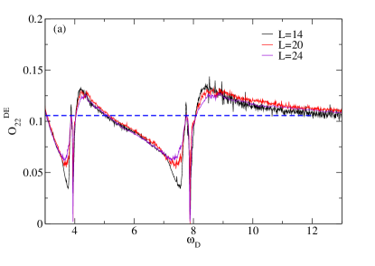
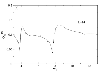
Figure 1: (a) Plots of $O_{22}^{\rm DE}$ as a function of the drive frequency starting from an initial state $|0\rangle$ for $L=14,18,24$. The blue dashed line indicates the infinite temperature thermal value of $O_{22}^{\rm DE}$ as predicted by ETH. The plots clearly indicate super-thermal and sub-thermal values of $O_{22}^{\rm DE}$ over a range of frequencies and dynamical freezing at specific frequencies where $O_{22}^{\rm DE}\simeq 0$. (b) Similar plot for $O_{22}^{DE}$ as a function of $\omega_{D}$ for $L=14$ as obtained using the analytic perturbative Floquet Hamiltonian given by Eqs. (12) and (17). All energies and frequencies are scaled in units of $w/\sqrt{2}$, $\hbar=1$, and $\lambda=15$ in rescaled units for all plots.

A plot of $O_{22}^{\rm DE}$, computed from the exact evolution operator, is shown in Fig. 1 (a) as a function of the drive frequency $\omega_{D}$. The corresponding plot, obtained starting from the analytical Floquet Hamiltonian at $\mathcal{O}(w^{3})$ (Eqs. (12) and (17)), is shown in Fig. 1 (b). From these plots, we note the following features. First, we find that $O_{22}^{\rm DE}$ obtained using the analytic Floquet Hamiltonian provides a qualitative match with that obtained from exact numerics. This brings out the importance of the multiple-spin term in Eq. (17); the PXP Floquet Hamiltonian (Eq. (12) and the single spin term in Eq. (17)), for dynamics starting from the $|0\rangle$ state, predict a featureless thermal value of $O_{22}^{\rm DE}$ as a function of $\omega_{D}$. Second, we note that $O_{22}^{\rm DE}$ reaches the expected infinite temperature thermal steady state value predicted by ETH (blue dashed line in Fig. 1) for high frequencies. This clearly indicates that $|\mathbb{Z}_{2}\rangle$ scars do not play a role in the dynamics. In contrast, at finite $\omega_{D}$, there are several non-ETH like features present as a function of the drive frequency at least up to $L=24$ (Fig. 1 (a)). Third, for $8\leq\omega_{D}\leq 12$, Fig. 1 (a) shows that $O_{22}^{DE}$ reaches super-thermal values; this phenomenon constitutes a violation of ETH for finite-sized chains $L\leq 24$. We shall discuss this feature in detail in Sec. III.1. Fourth, for $\omega_{D}\simeq 7.88,3.94..$, $O^{\rm DE}_{22}$ remains pinned to its initial value ($=0$); this constitutes an example of dynamical freezing at specific drive frequencies which we discuss in Sec. III.2. Finally, for $5\leq\omega_{D}\leq 7.5$, we find that $O_{22}^{\rm DE}$ exhibits sub-thermal steady-state values. This constitutes another class of violation of ETH for finite chains which we discuss in Sec. III.3. We note that the time evolution of $O_{22}$ as a function of the number of drive cycles, shown in Fig. 2, in these three regimes shows qualitatively distinct behaviors which can be discerned in realistic experiments involving Rydberg atom chains.

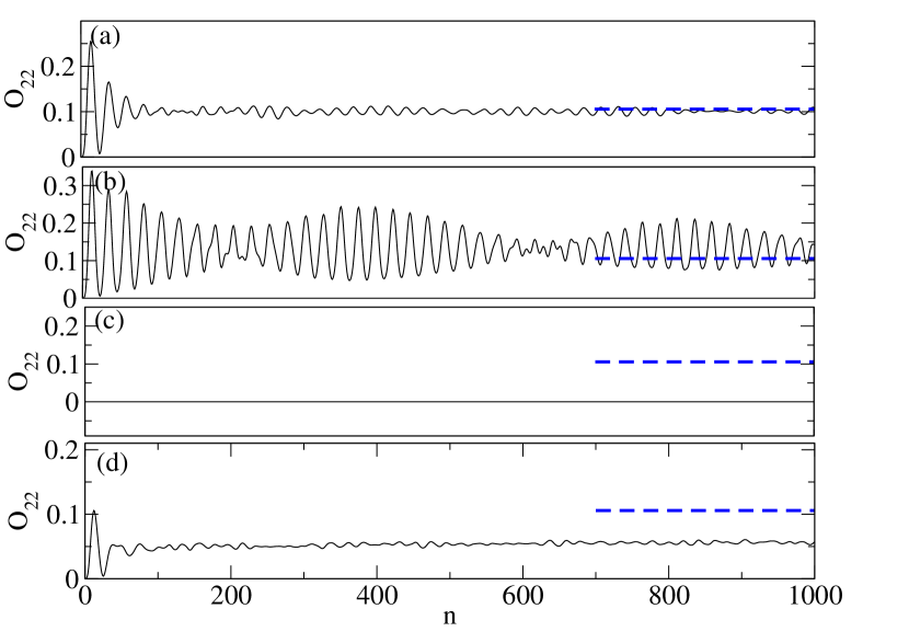
Figure 2: Plots of $O_{22}$ as a function of the number of drive cycles $n$ (stroboscopic time) starting from an initial state $|0\rangle$ for (a) $\omega_{D}=100$, (b) $\omega_{D}=8.5$, (c) $\omega_{D}=7.88$, and (d) $\omega_{D}=7.26$. The blue dashed line indicates the ETH predicted thermal value of $O_{22}$. Here $L=26$, $\lambda=15$, and all units are the same as in Fig. 1.

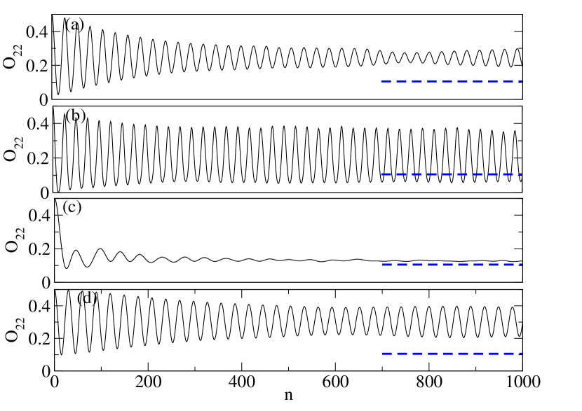
Figure 3: Plots of $O_{22}$ as a function of the number of drive cycles $n$ (stroboscopic time) starting from an initial state $|Z_{2}\rangle$ for (a) $\omega_{D}=100$, (b) $\omega_{D}=8.5$, (c) $\omega_{D}=7.88$, and (d) $\omega_{D}=7.26$. The blue dashed line indicates the ETH predicted thermal value of $O_{22}$. Here $L=26$, $\lambda=15$, and all units are the same as in Fig. 1

III.1 Super-thermal steady state value

The stroboscopic time evolution of $O_{22}$ starting from the $|0\rangle$ state is shown in Fig. 2 for $L=26$. The corresponding behavior of the same correlator starting from the $|\mathbb{Z}_{2}\rangle$ state is shown in Fig. 3. First, we note that for high frequencies such as $\omega_{D}=100$, Fig. 2 (a) shows expected thermalization while Fig. 3 (a) shows scar-induced oscillations. This behavior is consistent with earlier studies of the PXP model scarref2a ; scarref2b ; scarref2c ; scarref2d ; scarfl1 which reported thermalization for dynamics starting from the $|0\rangle$ state in cases of both quench and periodic protocol at high drive frequency. Panel (b) for Figs. 2 and 3, in contrast, indicate the presence of persistent oscillations for $\omega_{D}=8.5$ for dynamics starting from both $|0\rangle$ and $|\mathbb{Z}_{2}\rangle$ states. This leads to weak violation of ETH and super-thermal value of $O_{22}^{\rm DE}$ for dynamics starting from the $|0\rangle$ state.

To understand the origin of these oscillations, we show the half-chain entanglement entropy $S_{L/2}$ of the eigenstates $|\chi_{m}\rangle$ of the Floquet Hamiltonian for $\omega_{D}=8.5$ in Fig. 4 (a). The details of this computation have been charted out in Ref. scarfl1, . Fig. 4 (b) shows the value of

$$O_{22}^{m}=\frac{1}{4}\langle\chi_{m}|(1+\sigma_{2}^{z})(1+\sigma^{z}_{4})|\chi_{m}\rangle$$ (21)

for all Floquet eigenstates $|\chi_{m}\rangle$ as a function of the Floquet quasienergies $E_{F}$. The dotted line in this plot indicates the ETH value of $O_{22}$ at a temperature $T_{0}(E_{F})$ as a function of these quasienergies. Here $T_{0}(E_{F})$ is defined such that the average quasienergy equals $E_{F}$ for a canonical ensemble with temperature $T_{0}(E_{F})$.

Fig. 4 (a) shows the usual thermal ETH band with large $S_{L/2}$ along with sub-thermal states with lower values of $S_{L/2}$. The states $|\chi_{m}\rangle$ with $|\langle 0|\chi_{m}\rangle|^{2}(|\langle Z_{2}|\chi_{m}\rangle|^{2})>0.01$ which control the dynamics starting from the $|0\rangle(|Z_{2}\rangle)$ state is shown in red (green) circles in both panels. From Fig. 4 (a), we find that the low-entropy eigenstates of $H_{F}$ which control the dynamics are distinct for $|0\rangle$ and $|\mathbb{Z}_{2}\rangle$ initial states; at $\omega_{D}=8.5$, these states coexist with each other. Furthermore, the low-entropy eigenstates with large overlap with the $|0\rangle$ show values of $O_{22}^{m}$ closer to the ETH line compared to their counterpart for the $|\mathbb{Z}_{2}\rangle$ state as can be clearly seen from Fig. 4 (b); thus we expect $O_{22}^{\rm DE}$ starting from the $|0\rangle$ state to be closer to the ETH value compared to its $|\mathbb{Z}_{2}\rangle$ counterpart. Nevertheless, a finite number of these eigenstates contributing to the $|0\rangle$ dynamics are not thermal as can be seen from Fig. 4 (a). They have significantly lower values of $S_{L/2}$ compared to the eigenstates in the thermal band, and lead to persistent coherent oscillatory dynamics of $O_{22}$ starting from the $|0\rangle$ state. We therefore dub these states as $|0\rangle$ scars. Our findings indicate that there are at least two distinct types of scars in the Floquet spectrum of $H_{\rm spin}$ driven by the square pulse protocol given in Eq. (5); this phenomenon has no analog in the PXP model studied earlier where only $|\mathbb{Z}_{2}\rangle$ scars exist. We further note that the energy spacings between these $|0\rangle$ scar states are non-uniform unlike their $|\mathbb{Z}_{2}\rangle$ counterparts; this causes a strong beating phenomenon in the oscillation of $O_{22}$ (Fig. 2 (b)) which is much weaker for the corresponding $|\mathbb{Z}_{2}\rangle$ dynamics (Fig. 3 (b)). This can be more clearly seen in Fig. 5 where the Fourier transform of $O_{22}$ starting from $|0\rangle$ (Fig. 2 (b)) and from $|\mathbb{Z}_{2}\rangle$ (Fig. 3 (b)) are shown in Fig. 5 (a) and Fig. 5 (b) respectively.

As $\omega_{D}$ is increased, we find that the $|0\rangle$ scars merge with the thermal band and cannot be distinguished from them for $\omega_{D}>12$ where $O_{22}$ starts displaying thermal behavior consistent with ETH (Fig. 2 (a)); in contrast, the $|\mathbb{Z}_{2}\rangle$ scars persist at arbitrary high frequency (Fig. 3 (a)). This clearly demonstrates that the $|0\rangle$ scars require higher spin terms in $H_{F}$ such as the first term of Eq. (17); they are not eigenstates of the high frequency Floquet Hamiltonian which constitutes a renormalized PXP model. Finally, it is important to note here that the $|0\rangle$ scars have a higher entanglement entropy compared to their $|\mathbb{Z}_{2}\rangle$ counterparts (Fig. 4 (a)) and thus they may be more fragile to increasing system sizes.

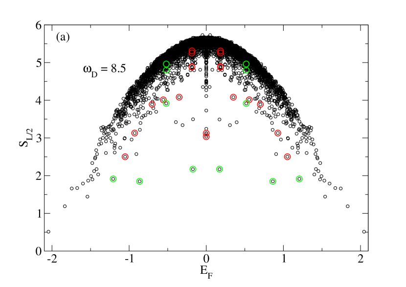
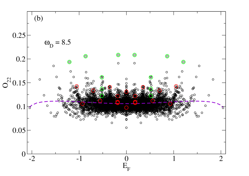
Figure 4: (a) Plot of $S_{L/2}$ for the eigenstates of $H_{F}$ for $L=26$ and $\omega_{D}=8.5$ at $\lambda=15$. The eigenstates with overlap $>0.01$ with $|0\rangle~{}(|\mathbb{Z}_{2}\rangle)$ are shown using red (green) circles. These states are distinct and coexist at this drive frequency. (b) Plot of $O_{22}^{m}$ as a function of Floquet eigenstate quasienergies $E_{F}$. The violet dashed line indicates the ETH predicted value of $O_{22}$ at a temperature $T_{0}(E_{F})$. All units are the same as in Fig. 1.

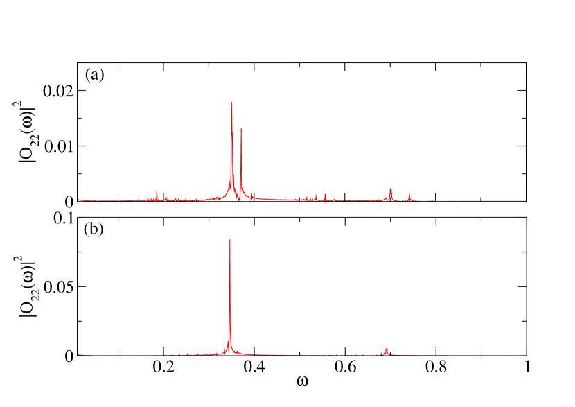
Figure 5: Plots of $|O_{22}(\omega)|^{2}$ obtained from the Fourier transforms of $O_{22}(n)$ for $L=26$, $\omega_{D}=8.5$ and $\lambda=15$ for the initial state being (a) $|0\rangle$ and (b) $|\mathbb{Z}_{2}\rangle$ respectively. All units are the same as in Fig. 1.

The role of the three or higher-spin terms in $H_{F}$ for the stability of $|0\rangle$ scars and the consequent coherent oscillations can be qualitatively understood using the FSA. To this end, we consider an effective Hamiltonian

$$H_{1}=-\sum_{j}\tilde{\sigma}^{x}_{j}+h\sum_{j}(\tilde{\sigma}^{+}_{j}\tilde{\sigma}^{-}_{j-1}\tilde{\sigma}^{-}_{j+1}+{\rm H.c.}),$$ (22)

which qualitatively mimics $H_{F}$ found in Sec. II, albeit with real valued coefficient $h$. Here we use $h$ as a tuning parameter and study the properties of the scar-induced oscillations within the FSA starting from $|0\rangle$. For this, we write $H_{1}=H^{+}+H^{-}$ (with $H^{-}=(H^{+})^{\dagger}$) and choose $H^{-}=-w\sum_{j}\tilde{\sigma}^{-}_{j}+h\sum_{j}\tilde{\sigma}^{+}_{j}\tilde{\sigma}^{-}_{j-1}\tilde{\sigma}^{-}_{j+1}$ so that $H^{-}|0\rangle=0$. The repeated application of $H^{+}$ on $|0\rangle$ (forward scattering) then generates a closed Krylov subspace. Following standard procedure, we designate a particular forward scattering step to be exact when the action of $H^{+}$ on the Krylov vector in that step can be totally reversed by the action of $H^{-}$. The inexact FSA steps generate errors which we aim to minimize. The details of this analysis is charted out in App. C. The main results that come out of this analysis are as follows. First, we find that in the bare PXP model ($H_{1}(h=0)$) all forward scattering action are inexact after the first two FSA steps; these errors cannot be minimized for $h=0$. This shows that the FSA predicts instability of the $|0\rangle$ scars within the PXP model. Second, we find that $h$ provides a control knob which can minimize the FSA errors at different steps, although there is no common value of $h$ for which errors in all the FSA steps are simultaneously minimized. Our analysis finds that the errors for the third FSA step (which is also the first error generating FSA step) is minimized for $h^{\rm min}\simeq 0.3$; furthermore, errors in other FSA steps are minimum close to (but not exactly at) $h=h^{\rm min}$. The details of this procedure and the $L$ dependence of this result is detailed out in App. C. Our analysis thus brings out the importance of higher-spin terms in $H_{1}$ (and $H_{F}$) for the stability of $|0\rangle$ scars. Finally, we find that the addition of further terms such as a five-spin term to $H_{1}$ (see App. C) can lead to further amplification of scar-induced oscillations and chart out the values of coefficients which achieves such amplification. The Floquet Hamiltonian $H_{F}$ provides a natural setting for generating such longer-ranged terms as the drive frequency $\omega_{D}$ is lowered.

III.2 Dynamical freezing

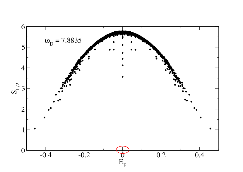
Figure 6: Plot of $S_{L/2}$ for the eigenstates of $H_{F}$ for $L=26$ and $\omega_{D}=7.8835$ at $\lambda=15$. The state encircled in red shows the presence of a quantum scar with a very high overlap ($>0.9999$) with the $|0\rangle$ state. All units are the same as in Fig. 1.

For $\omega_{D}=7.88$, we find from Fig. 2 (c), that the $|0\rangle$ state, in spite of not being an eigenstate of $H_{F}$, does not exhibit almost any time evolution. This phenomenon is also found for other lower, subharmonic, drive frequencies as seen in Fig. 1 (a) where $O_{22}^{\rm DE}$ exhibits a sharp dip to $0$. This is in sharp contrast to the evolution of the $|\mathbb{Z}_{2}\rangle$ state which shows thermalization at this frequency (Fig. 3 (c)) scarfl1 . This behavior constitutes an example of dynamical freezing which we now discuss. At these dynamic freezing frequencies, a quantum scar state with vanishingly small entanglement has an almost perfect overlap ($>0.9999$ till $L=26$) with the $|0\rangle$ state as shown by the behavior of $S_{L/2}$ in Fig. 6.

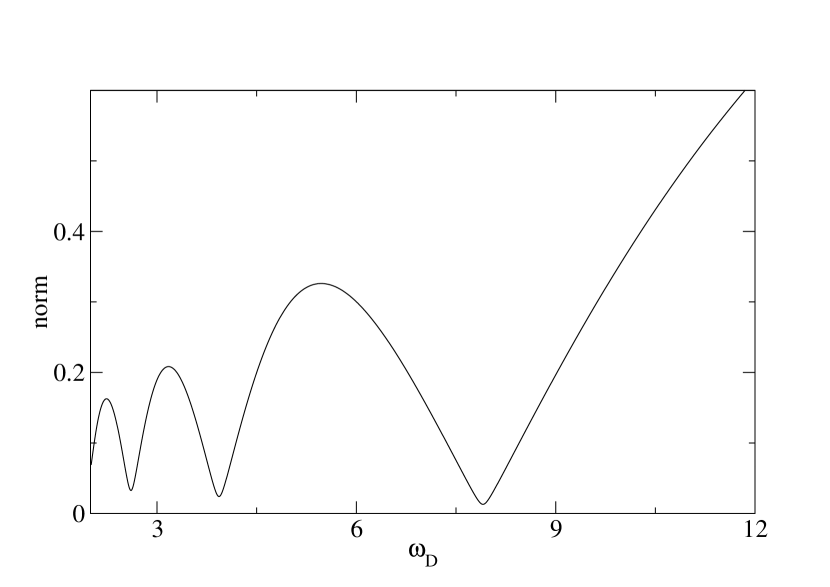
Figure 7: Plot of the norm ${\mathcal{N}}$ as a function of $\omega_{D}$. Here $\lambda=15$ and all units are the same as in Fig. 1. See text for details.

We first obtain a qualitative understanding of this phenomenon using the Floquet Hamiltonian given by Eqs. (12) and (17). To this end we note that $\tilde{\sigma}_{j}^{-}|0\rangle=0$ for any $j$. Thus the first term in Eq. (17) (and any higher order terms in $H_{F}$ which have $\tilde{\sigma}_{j}^{-}$) annihilates the state $|0\rangle$. Consequently, the only non-trivial terms in $H_{F}$ contributing to the evolution of the $|0\rangle$ state are the single spin terms charted out in Eqs. (12) and (17). These single spin terms can be written as

$$H_{F}^{\rm single} = -\sum_{j}\Big{[}\left(w\frac{\sin(2\gamma)}{2\gamma}+6{\rm Re}[A_{0}]\right)\tilde{\sigma}_{j}^{x}$$ (23)

$$\quad\quad\quad+\left(w\frac{\sin^{2}\gamma}{\gamma}-6{\rm Im}[A_{0}]\right)\tilde{\sigma}^{y}_{j}\Big{]}$$

$$= \sum_{j}~{}(C_{1}\tilde{\sigma}_{j}^{x}+C_{2}\tilde{\sigma}_{j}^{y}).$$

For drive frequencies where the norm ${\mathcal{N}}=\sqrt{C_{1}^{2}+C_{2}^{2}}$ of these terms is close to zero, we expect $|\psi(T)\rangle=U(T,0)|0\rangle\simeq|0\rangle$. We find, as shown in Fig. 7, that ${\mathcal{N}}$ comes very close to zero (although it does not vanish, in contrast to exact numerics) around $\omega_{D}\simeq 7.9$ which is remarkably close to the freezing frequency observed in exact numerics.

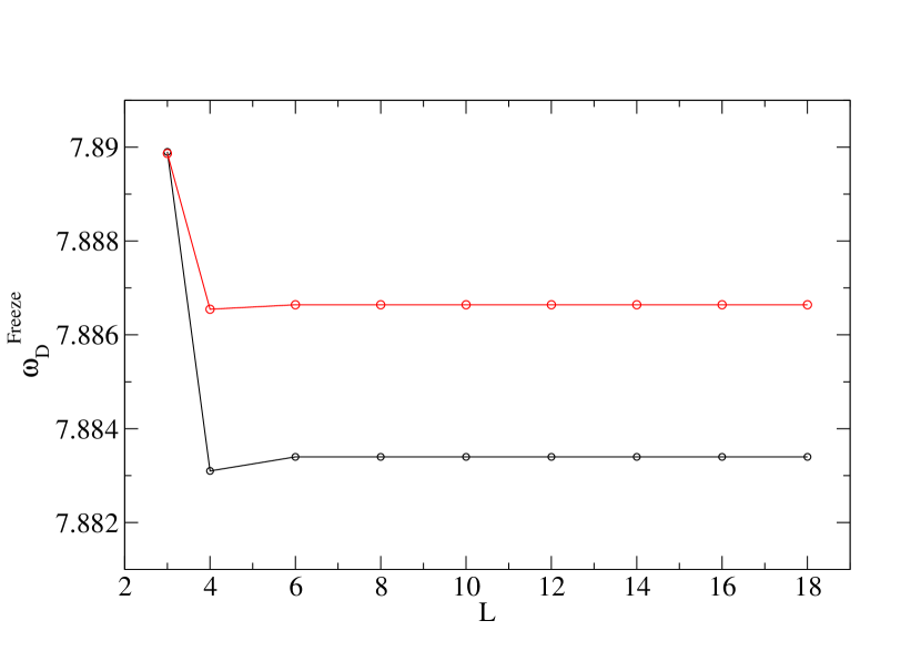
Figure 8: Plot of $\Delta_{0}/2$ (black solid line) and the highest freezing frequency $\omega_{D}^{\rm freeze}$ (red solid line) as a function of $L$. Here $\lambda=15$ and all units are the same as in Fig. 1.

The above perturbative analysis indicates that multiple spin terms do not play an essential role in the freezing phenomenon since, at least to $O(w^{3})$, all of them annihilate the $|0\rangle$ state. Thus it is natural to expect that this phenomenon can also be qualitatively understood by focussing on small system sizes where the small size of the Hilbert space allows for an exact analytical calculation. To this end, we consider a $L=3$ system. In the $k=0$ sector, there are two states in its constrained Hilbert space. These are $|0\rangle=|\downarrow\downarrow\downarrow\rangle$, and $|1\rangle=(|\uparrow\downarrow\downarrow\rangle+|\downarrow\uparrow\downarrow\rangle+|\downarrow\downarrow\uparrow\rangle)/\sqrt{3}$. In the space of these states, the Hamiltonian can be written, up to an irrelevant constant term, as

$$H[\pm\lambda]=\left(\begin{array}[]{cc}0&-\sqrt{3}w\\ -\sqrt{3}w&\pm\lambda\\ \end{array}\right).$$ (24)

The Floquet Hamiltonian for this system can be computed exactly and is given by

$$H_{F}^{\rm exact} = \frac{ic}{T\sin(c)}\Big{[}\frac{2\sqrt{3}w\sin(\Delta_{0}T/2)}{\Delta_{0}}\tau_{x}$$ (25)

$$\quad\quad\quad\quad-\frac{4\sqrt{3}w\lambda\sin^{2}(\Delta_{0}T/4)}{\Delta_{0}^{2}}\tau_{y}\Big{]},$$

where $\tau^{x,y}$ denotes Pauli matrices in the space of states $|0\rangle$ and $|1\rangle$, $\Delta_{0}=\sqrt{12w^{2}+\lambda^{2}}$ is the static energy gap between the states $|0\rangle$ and $|1\rangle$ states, and $c=\cos^{-1}(1-24w^{2}\sin^{2}(\Delta_{0}T/4)/\Delta_{0}^{2})$. This leads to the expression for the matrix element between the states $|0\rangle$ and $|1\rangle$ as

$$|\langle{0}|H_{F}^{\rm exact}|{1}\rangle|=\frac{\omega_{D}}{2\pi}\cos^{-1}\left[\frac{\lambda^{2}+12w^{2}\cos\left(\Delta_{0}T/2\right)}{\Delta_{0}^{2}}\right].$$ (26)

This shows that for $\omega_{D}=\omega_{D}^{\rm freeze}=\Delta_{0}/(2m)$, where $m$ is an integer, the matrix element between $|0\rangle$ and $|1\rangle$ exactly vanishes. Consequently, $|0\rangle$ does not evolve at these frequencies. Thus the freezing frequencies are directly related to the static gap $\Delta_{0}$ between the $|0\rangle$ and the single up-spin ($|1\rangle$) states. We note that our analytic expression for $\omega_{D}^{\rm freeze}$ provides a natural explanation for the subharmonic structure of the lower freezing frequencies. These frequencies turn out to match almost exactly with ED based numerical computation for finite $L\leq 26$. This is shown in Fig. 8 where $\Delta_{0}/2$ and the highest $\omega_{D}^{\rm freeze}$ ($m=1$) is plotted as a function of $L$. The reason for this near-perfect match is that multiple spin terms in $H_{F}$ do not contribute to this phenomenon as explained earlier. We also supplement this numerical check by an explicit analytic calculation for $L=4$ in App. B.

III.3 Sub-thermal steady state value

In this section, we address the sub-thermal behavior of the system as seen, for example, in the frequency range $5\leq\omega_{D}\leq 7.5$. Throughout this range, the dynamics of the system, starting from the $|0\rangle$ state, is qualitatively identical to that shown in Fig. 2 (d). It shows a rapid approach to a steady state where $O_{22}$ assumes a sub-thermal value; in addition, there are no persistent coherent oscillations, in contrast to the $|\mathbb{Z}_{2}\rangle$ dynamics shown in Fig. 3 (d). This behavior constitutes a novel route to a violation of ETH in finite-sized systems for two reasons. First, we do not see here the persistent oscillations usually seen in dynamics controlled by quantum scars, and second, $O_{22}$ assumes sub-thermal, in contrast to super-thermal, values in the steady state.

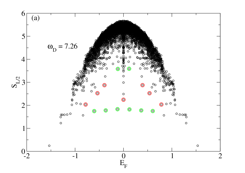
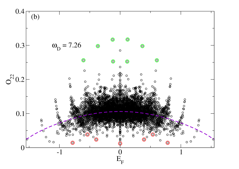
Figure 9: (a) Plot of $S_{L/2}$ for the eigenstates of $H_{F}$ for $L=26$ and $\omega_{D}=7.26$. The eigenstates with overlap $>0.01$ with $|0\rangle~{}(|Z_{2}\rangle)$ are shown using red (green) circles. (b) Plot for $O_{22}^{m}$ as a function of Floquet eigenstate quasienergies $\epsilon_{F}$. The violet dashed line indicates the ETH predicted value of $O_{22}$ at a temperature $T_{0}(E_{F})$. Here $L=26$, $\lambda=15$ and all units are the same as in Fig. 1.

To understand this phenomenon, we plot $S_{L/2}$ for the eigenstates of $H_{F}$ for $\omega_{D}=7.26$ in Fig. 9 (a) and $O_{22}^{m}$ as a function of Floquet quasienergies in Fig. 9 (b). From both these panels, we note that there are relatively few sub-thermal states with high overlaps with the $|0\rangle$ state; in particular, there are no thermal states with overlap $|\langle\chi_{m}|0\rangle|^{2}>0.01$ at this frequency. Thus the weight of the $|0\rangle$ state is distributed among a few sub-thermal and a relatively large set of thermal states. The dynamics starting from the $|0\rangle$ state within this frequency range is analogous to a quantum system coupled to a bath which features a large range of incommensurate natural frequencies; the presence of a large number of thermal states which have small but finite overlaps with $|0\rangle$ mimics the effect of a bath in the present context. The presence of such a bath leads to fast decoherence of the oscillations and leads to a steady state. This behavior is in stark contrast to the dynamics at $\omega_{D}=8.5$ where a few sub-thermal states with large overlaps control the dynamics.

The sub-thermal values of $O_{22}$ in this steady state are more difficult to explain. Numerically, from Fig. 9 (b), we find that the Floquet eigenstates with relatively large overlaps with the $|0\rangle$ state have sub-thermal values of $O_{22}^{m}$, and this feature is opposite to that for states with large overlaps with $|\mathbb{Z}_{2}\rangle$. From Eq. (20), we expect that this feature will lead to sub-thermal values of $O_{22}$ in the steady state. However, beyond this observation, we do not have a more analytical explanation for this phenomenon. We also note that such sub-thermal values of $O_{22}$ in the steady state are clearly a finite-size effect; for $L\to\infty$, the number of thermal Floquet eigenstates with finite overlap with $|0\rangle$ will be exponentially larger than the sub-thermal states and their contribution is expected to lead to the ETH predicted thermal value of $O_{22}$ in the steady state. However, for all $L\leq 26$ we do not find thermal behavior; moreover for this range of system sizes, the steady state value of $O_{22}$ remains almost constant as can be seen from the values of $O_{22}^{DE}$ for $L=14,~{}20,\,{\rm and}\,24$ in Fig. 1. This indicates that a restoration of ETH is expected only for $L\gg 26$; for $L\leq 26$, we find a qualitatively distinct and experimentally discernible characteristic of $O_{22}$ which is different from both scar-induced persistent oscillations and ETH predicted thermalization. Furthermore, the behavior of $O_{22}$ as a function of $n$ upto $1000$ drive cycles for different system sizes (Fig. 10) suggests that this non-ETH sub-thermal behavior can persist as a prethermal regime for reasonably large $n$ before the system eventually flows to an ITE even for much larger system sizes. We therefore believe that this phenomenon provides a novel route to ETH violation in a finite-sized Rydberg chain.

Figure 10: Plots of $O_{22}$ as a function of the number of drive cycles $n$ (stroboscopic time) starting from an initial state $|0\rangle$ for $L=20$ (green), $L=24$ (red), and $L=26$ (black), for $\omega_{D}=7.26$ and $\lambda=15$. The blue dashed line indicates the ETH predicted thermal value of $O_{22}$. All units are the same as in Fig. 1.

IV Discussion

In this work, we have studied the dynamics of a periodically driven Rydberg chain starting from the $|0\rangle$ state using a square pulse protocol. Our study involves exact numerics on finite-sized chains and a perturbative Floquet Hamiltonian based analysis whose analytic expression is derived using Floquet perturbation theory in the high drive amplitude limit.

Our study indicate three distinct behaviors of such dynamics. First, we show that dynamics starting from the $|0\rangle$ state can exhibit scar-induced persistent oscillations over a range of drive frequencies $8\leq\omega_{D}\leq 12$. These scars are distinct from their $\mathbb{Z}_{2}$ counterparts; they are absent in the high drive frequency limit and are not eigenstates of the (renormalized) PXP Hamiltonian studied earlier in the literature scarfl1 ; scarref1 ; scarref2a ; scarref2b ; scarref2c ; scarref2d ; scarref2e . They coexist with the $|\mathbb{Z}_{2}\rangle$ scars in the above-mentioned drive frequency range. These $|0\rangle$ scars have higher entanglement than their $|\mathbb{Z}_{2}\rangle$ counterparts and seem more fragile to increasing system sizes. It will be worthwhile to understand perturbations that may further reduce the entanglement of these $|0\rangle$ scars.

Second, for specific drive frequencies $\omega_{D}^{\rm freeze}\simeq 7.88,3.94,\cdots$, we find that the system exhibits dynamic freezing. We provide an analytic, albeit qualitative, explanation of this phenomenon using the perturbative Floquet Hamiltonian and supplement it with exact analytic calculation at small system sizes $L=3$ and 4. Our analysis relates the freezing frequencies with the energy gap $\Delta_{0}$ between the $|0\rangle$ and $|1\rangle$ states: $\omega_{D}^{\rm freeze}=\Delta_{0}/2m$ for $m=1,2,3,\cdots$. This provides a natural explanation for the relation between several freezing frequencies and also provides a reasonably accurate estimate of these frequencies as can be seen by comparing the analytic result with exact numerics for all $L\leq 26$. We note that such a behavior has no analogue for dynamics starting from the $|\mathbb{Z}_{2}\rangle$ state. Such dynamical freezing should also be visible in the thermodynamic limit as prethermal freezing which only flows to an ITE after an exceptionally long time scale.

Third, we show that for $5\leq\omega_{D}\leq 7.5$, the system reaches a steady state with sub-thermal values of $O_{22}$ for all $L\leq 26$ which constitutes a violation of ETH. In contrast to the scar-induced weak violation of ETH, in this regime, the system does not exhibit persistent oscillations for $O_{22}$. We relate this behavior to the presence of small overlaps of a large number of Floquet eigenstates with the $|0\rangle$ state; this leads to the fast decay of coherent oscillations in $O_{22}$. Moreover, numerically we find that $O_{22}^{m}$ for many of the Floquet eigenstates which have high overlap with $|0\rangle$ assumes sub-thermal values; this leads to sub-thermal values of $O_{22}$ in the steady state. We note that such a violation of ETH is distinct from its counterpart in the dynamics starting from the $|\mathbb{Z}_{2}\rangle$ state; it does not feature persistent oscillations and leads to steady states with sub-thermal, rather than super-thermal, values of $O_{22}$. Our numerical results for finite-sized chains also suggest that this sub-thermal behavior can survive as a prethermal phase for finite but large number of drive cycles before the system eventually flows to an ITE in the thermodynamic limit.

All the above three features should be observable in realistic experiments with a Rydberg chain. The differences of our proposal with experiments already carried out in Ref. scarref1, are two-fold. First, for our proposal, we need to start from the $|0\rangle$ state. This is not difficult to implement since this state turns out to be the ground state of $H$ in Eq. (LABEL:ryd1) for large positive $\Delta$. Second, we need to implement a periodic variation of $\Delta$ according to the protocol given in Eq. (2) instead of a quench. Our prediction is that the dynamics starting from the $|0\rangle$ state will show persistent scar-induced oscillations, dynamic freezing and novel steady states featuring sub-thermal values of $C_{22}\equiv O_{22}$ in such experiments.

In conclusion, we have shown that dynamics starting from the $|0\rangle$ state in a finite-sized periodically driven Rydberg chain shows scar-induced oscillations, dynamic freezing, and steady states with sub-thermal value of correlators for various ranges of drive frequencies which we have charted out. The first feature shows that the Floquet Hamiltonian hosts two sets of coexisting scars; the last two phenomena have no analogs in periodic or quench dynamics involving the $|\mathbb{Z}_{2}\rangle$ initial state studied earlier. We have provided an analytic, albeit perturbative, Floquet Hamiltonian which explains these features qualitatively and have suggested experiments which can test our theory.

On a broader level, our work suggests the possibility of interesting prethermal Floquet phases at moderate and low drive frequencies in the high drive amplitude limit Vajna2018 . Such a prethermalization mechanism is quite distinct from the well-known long preheating times generated in Floquet systems when the driving frequencies are much bigger than the local energy scales Saito_etal and should lead to richer possibilities.

Appendix A Floquet perturbation theory

In this appendix, we sketch the essential points regarding the derivation of the Floquet Hamiltonian. For this purpose, we first note that, as explained in the text, $U_{0}$ is given by

$$U_{0}(t,0) = e^{i\lambda t\sum_{j}\sigma_{j}^{z}/2}\quad{\rm for}\quad t\leq T/2,$$ (27)

$$= e^{i\lambda(T-t)\sum_{j}\sigma_{z}^{j}/2}\quad{\rm for}\quad T/2\leq t\leq T.$$

Noting the form of $U_{0}$, we define the functions

$$I_{0}^{(1)}(t,s) = e^{i\lambda st},\quad I_{0}^{(2)}(t,T,s)=e^{i\lambda s(T-t)},$$

$$I_{1}(t,s) = \int_{0}^{t}dtI_{0}^{(1)}(t,s)=\frac{1}{i\lambda s}\left(e^{i\lambda st}-1\right),$$ (28)

$$I_{2}(t,T,s) = \int_{0}^{t}dtI_{0}^{(2)}(t,T,s)=\frac{e^{i\lambda sT}}{i\lambda s}\left(1-e^{-i\lambda st}\right).$$

where $s=\pm 1$. The first order term in the Floquet Hamiltonian $U_{1}=-i\int_{0}^{T}U_{0}^{\dagger}(t,0)H_{1}U_{0}(t,0)dt$ can be expressed in terms of these functions as

$$\langle U_{1}(T,0)\rangle_{m,n} = iw\sum_{s=\pm}\delta_{m,n+s}\Big{[}\int_{0}^{T/2}dtI_{0}^{(1)}(t,s)$$ (29)

$$+\int_{T/2}^{T}dtI_{0}^{(2)}(t,T,s)\Big{]}$$

$$= iw\delta_{m,n+s}\left[I_{1}(T/2,s)+I_{2}(T,T,s)\right]$$

$$= \frac{2w}{\lambda s}\delta_{m,n+s}\left(e^{i\lambda sT/2}-1\right),$$

which leads to the ${\rm O}(w)$ term in the Floquet Hamiltonian (Eq. (12)) as discussed in the main text.

Next, we evaluate the matrix elements of $U_{2}(T,0)=(-i)^{2}\int_{0}^{T}dt_{1}H_{I}(t_{1})\int_{0}^{t_{1}}dt_{2}H_{I}(t_{2})$, where $H_{I}=U_{0}^{\dagger}H_{1}U_{0}$ is the perturbative term in $H$ in the interaction picture, between two states $m$ and $n$. A straightforward calculation shows

$$\langle U_{2}(T,0)\rangle_{mn} = (iw)^{2}\sum_{s_{1}=\pm,s_{2}=\pm}\delta_{m,n+s_{1}+s_{2}}\left[\left(\int_{0}^{T/2}dtI_{0}^{(1)}(t_{1},s_{1})+\int_{T/2}^{T}dtI_{0}^{(2)}(t_{1},T,s_{1})\right)\right.$$ (30)

$$\times\left.\left(\int_{0}^{t_{1}}dt_{2}I_{0}^{(1)}(t_{2},s_{2})\theta(t_{1}-T/2)+\int_{T/2}^{t_{1}}dt_{2}I_{0}^{(2)}(t_{2},T,s_{2})\theta(T/2-t_{1})\right)\right].$$

To evaluate this expression we first define the integrals

$$I_{3}(t,s_{1},s_{2}) = \int_{0}^{t}dt_{1}I_{0}^{(1)}(t_{1},s_{1})I_{1}(t_{1},s_{2})=-\frac{1}{2\lambda^{2}}\left[\left(e^{i\lambda s_{1}t}-1\right)^{2}\delta_{s_{1},s_{2}}+\left(1-e^{i\lambda s_{1}t}+i\lambda s_{1}t\right)\delta_{s_{1},-s_{2}}\right],$$ (31)

$$I_{4}(t,T,s_{1},s_{2}) = \int_{T/2}^{t}dt_{1}I_{0}^{(2)}(t_{1},T,s_{1})I_{2}(t_{1},T,s_{2})=-\frac{1}{2\lambda^{2}}\left[e^{i\lambda s_{1}(2t-T)}\left(e^{i\lambda s_{1}t}-e^{i\lambda s_{1}T/2}\right)^{2}\delta_{s_{1},s_{2}}\right.$$

$$\quad\quad\quad\quad\quad\quad\quad\quad\quad\quad\quad\quad~{}\quad\quad\quad\quad\quad\quad\left.+\left(2(1-e^{i\lambda s_{1}(2t-T)})-i\lambda s_{1}(2t-T)\right)\delta_{s_{1},-s_{2}}\right].$$

In terms of these integrals, we can write

$$U_{2}(T,0) = \sum_{i,j}\sum_{s_{1},s_{2}=\pm}c^{(2)}_{s_{1}s_{2}}\sigma_{i}^{s_{1}}\sigma_{j}^{s_{2}},$$

$$c_{s_{1}s_{2}}^{(2)} = -w^{2}\left[I_{3}(T/2,s_{1},s_{2})~{}+~{}I_{4}(T,T,s_{1},s_{2})\right.$$ (32)

$$\left.~{}~{}~{}~{}~{}~{}+~{}I_{2}(T,T,s_{1})I_{1}(T,s_{2})\right].$$

Using Eqs. (32) and (31), we find that

$$c_{s,s}^{(2)} = \frac{2w^{2}}{\lambda^{2}}\left(e^{i\lambda sT/2}-1\right)^{2},$$

$$c_{s,-s}^{(2)} = -\frac{8w^{2}}{\lambda^{2}}\sin^{2}(\lambda T/4),$$ (33)

which are used in the main text.

Finally, we address the third order term given in Eq. (15). In terms of the functions $I_{0}^{(1)}$ and $I_{0}^{(2)}$ these can be written as

$$\langle U_{2}(T,0)\rangle_{mn} = (-iw)^{3}\sum_{s_{1},s_{2},s_{3}=\pm}\delta_{m,n+s_{1}+s_{2}+s_{3}}\left[\left(\int_{0}^{T/2}dtI_{0}^{(1)}(t_{1},s_{1})+\int_{T/2}^{T}dtI_{0}^{(2)}(t_{1},T,s_{1})\right)\right.$$ (34)

$$\times\left.\left(\int_{0}^{t_{1}}dt_{2}I_{0}^{(1)}(t_{2},s_{2})\theta(t_{1}-T/2)+\int_{T/2}^{t_{1}}dt_{2}I_{0}^{(2)}(t_{2},T,s_{2})\theta(T/2-t_{1})\right)\right.$$

$$\left.\times\left(\int_{0}^{t_{2}}dt_{3}I_{0}^{(1)}(t_{3},s_{3})\theta(t_{2}-T/2)+\int_{T/2}^{t_{2}}dt_{3}I_{0}^{(2)}(t_{3},T,s_{3})\theta(T/2-t_{2})\right)\right].$$

Evaluating Eq. (34) carefully after taking care of all commutators, we obtain

$$U_{3}(T,0) = \sum_{j,j^{\prime},j"}\sum_{m}\sum_{s_{1},s_{2},s_{3}=\pm}c^{(3)}_{s_{1}s_{2}s_{3}}\tilde{\sigma}_{j}^{s_{1}}\tilde{\sigma}_{j^{\prime}}^{s_{2}}\tilde{\sigma}_{j"}^{s_{3}},$$

$$c^{(3)}_{s_{1},s_{2},s_{3}} = \sum_{i}\alpha_{i}(T,s_{1},s_{2},s_{3}),$$

$$\alpha_{1}(T,s_{1},s_{2},s_{3}) = \int_{0}^{T/2}dtI_{0}^{(1)}(t_{1},s_{1})I_{3}(t,s_{1},s_{2}),$$

$$\alpha_{2}(T,s_{1},s_{2},s_{3}) = \int_{T/2}^{T}dtI_{0}^{(2)}(t_{1},Ts_{1})I_{4}(t,T,s_{1},s_{2}),$$

$$\alpha_{3}(T,s_{1},s_{2},s_{3}) = I_{2}(T,T,s_{1})I_{3}(T/2,s_{2},s_{3}),$$ (35)

$$\alpha_{4}(T,s_{1},s_{2},s_{3}) = I_{2}(T,T,s_{1})I_{2}(T,T,s_{2})I_{1}(T/2,s_{3}).$$

The integrals $\alpha_{1,2}$ lead to cumbersome expressions but can be straightforwardly obtained using Mathematica. Evaluating these integrals and using Eqs. (28) and (31), we finally obtain the coefficients $c_{s_{1},s_{2},s_{3}}^{(3)}$ used in the main text.

Appendix B Freezing frequencies for $L=4$

In this Appendix, we consider a $L=4$ system and provide an analytical expression for the freezing frequencies. It turns out that $L=4$ is the lowest value of $L$ for which the Hilbert space has a two-particle manifold and has dimension $6$. The $k=0$ sector has only three states given by

$$|{0}\rangle = |{0000}\rangle,$$

$$|{1}\rangle = \frac{1}{2}(|{1000}\rangle+|{0100}\rangle+|{0010}\rangle+|{0001}\rangle),$$

$$|{2}\rangle = \frac{1}{\sqrt{2}}(|{1010}\rangle+|{0101}\rangle),$$ (36)

where $|0\rangle~{}(|1\rangle)=|\downarrow\rangle~{}(|\uparrow\rangle)$. In this subspace the Hamiltonian $H_{\rm spin}[\pm\lambda]$ can be written as

$$H_{\pm}=\left(\begin{array}[]{ccc}0&2w&0\\ 2w&\pm\lambda&\sqrt{2}w\\ 0&\sqrt{2}w&\pm 2\lambda\\ \end{array}\right).$$ (37)

It is quite difficult to explicitly calculate $H_{F}$ from Eq. (37) for the square pulse protocol. Instead we will provide an analytic expression for $U_{11}(T,0)$. It is easy to see that this is equivalent to computing $|\langle{0}|H_{F}|{1}\rangle|$ for the purpose of locating the freezing frequencies. The argument goes as follows. The fidelity after one cycle $|\langle{0}|U(T)|{0}\rangle|^{2}=U_{11}$ should be unity at the freezing points. So $U_{11}(T,0)=1$ acts as an identifier of the freezing points.

To this end, we first compute the eigenspectrum of $H[\pm\lambda]$. The eigenvalues of $H[\lambda]$ are given by

$$\epsilon_{1} = w~{}[n~{}+~{}2R^{1/3}\cos(\alpha/3)],$$

$$\epsilon_{2} = w~{}[n~{}-~{}2R^{1/3}\cos((\alpha+\pi)/3)],$$

$$\epsilon_{3} = w~{}[n~{}-~{}2R^{1/3}\cos((\alpha-\pi)/3)],$$ (38)

where $n=\lambda/w$ , $R=(n^{2}/3+2)^{3/2}$, and $\alpha=\tan^{-1}(-R/n)$. It turns out that the eigenvalues of $H[-\lambda]$ are $-\epsilon_{1,2,3}$. The corresponding normalized eigenstates of $H[\pm\lambda]$ are given by

$$|{\psi^{\pm\lambda}_{i}}\rangle = \frac{1}{N_{i}}\left(\begin{array}[]{c}1\\ \pm\epsilon_{i}/2w\\ (1-\frac{2\lambda}{\epsilon_{i}})^{-1}/\sqrt{2}\end{array}\right),$$ (42)

$$N_{i} = \sqrt{1+\frac{\epsilon_{i}^{2}}{4w^{2}}+\frac{\epsilon_{i}^{2}}{2(\epsilon_{i}-2\lambda)^{2}}}.$$ (43)

Using the eigenspectrum of $H[\pm\lambda]$, we can obtain an expression for $U_{11}(T,0)$. A straightforward calculation yields

$$U_{11} = \frac{1}{4}\Big{(}\frac{\epsilon_{1}^{2}\left(\frac{2}{(\epsilon_{1}-2\lambda)^{2}}-\frac{1}{w^{2}}\right)+4}{N_{1}^{4}}+\frac{\epsilon_{2}^{2}\left(\frac{2}{(\epsilon_{2}-2\lambda)^{2}}-\frac{1}{w^{2}}\right)+4}{N_{2}^{4}}+\frac{\epsilon_{3}^{2}\left(\frac{2}{(\epsilon_{3}-2\lambda)^{2}}-\frac{1}{w^{2}}\right)+4}{N_{3}^{4}}$$

$$+ \frac{2\cos\left(\frac{1}{2}T(\epsilon_{1}-\epsilon_{3})\right)\left(\epsilon_{1}\epsilon_{3}\left(\frac{2}{(\epsilon_{1}-2\lambda)(\epsilon_{3}-2\lambda)}-\frac{1}{w^{2}}\right)+4\right)}{N_{1}^{2}N_{3}^{2}}+\frac{2\cos\left(\frac{1}{2}T(\epsilon_{2}-\epsilon_{3})\right)\left(\epsilon_{2}\epsilon_{3}\left(\frac{2}{(\epsilon_{2}-2\lambda)(\epsilon_{3}-2\lambda)}-\frac{1}{w^{2}}\right)+4\right)}{N_{2}^{2}N_{3}^{2}}$$

$$+ \frac{2\cos\left(\frac{1}{2}T(\epsilon_{1}-\epsilon_{2})\right)\left(\epsilon_{1}\epsilon_{2}\left(\frac{2}{(\epsilon_{1}-2\lambda)(\epsilon_{2}-2\lambda)}-\frac{1}{w^{2}}\right)+4\right)}{N_{1}^{2}N_{2}^{2}}\Big{)}.$$

Analyzing this expression, we find that $U_{11}(T,0)\simeq 1$ for $\cos\left(\Delta_{0}T/2\right)=1$, where $\Delta_{0}=\epsilon_{2}-\epsilon_{1}$ in spite of the complicated expression for $U_{11}(T,0)$ (see Fig. 11) when $\lambda\gg w$. This yields $\omega_{D}^{\rm freeze}=\Delta_{0}/(2m)$. Thus the freezing condition is identical to the result for $L=3$ given in the main text.

Figure 11: Curves for $U_{11}(T,0)$ using Eq. (LABEL:U11eq) (in black) and $\cos(\Delta_{0}T/2)$ (in red) as a function of $\omega_{D}$ show that the drive frequencies at which $U_{11}(T,0)=1$ and $\cos(\Delta_{0}T/2)=1$ almost coincide (see inset for details) when $\lambda\gg w$.

Appendix C FSA from $|0\rangle$

In this appendix, we shall chart out the FSA formalism using $|0\rangle$ as the starting state. In Sec. C.1, we demonstrate the computation using the PXP model while in Sec. C.2, we add higher spin terms to the Hamiltonian used for the FSA analysis.

C.1 FSA in the PXP model

In this section we carry out the FSA analysis using the PXP model starting from $|0\rangle$. We decompose the PXP Hamiltonian

$$H_{PXP}=w\sum_{i=1}^{L}\tilde{\sigma}^{x}_{i}=w\sum_{i}(\tilde{\sigma}^{+}_{i}+\tilde{\sigma}^{-}_{i})=H^{+}+H^{-}.$$ (45)

We assume $w=1$ and hence drop it from all further calculations in this section. This decomposition is motivated by the requirement that $H^{-}$ should annihilate the initial state ($|0\rangle$) and $H^{+}$ should annihilate the final state ($|{\mathbb{Z}}_{2}\rangle$ and $|\bar{{\mathbb{Z}}_{2}}\rangle$). This leads to the modified Lanczos operation acting in the Krylov space spanned by $L/2+1$ states (for system size $L$) obtained via repeated action of $H^{+}$ on the state $|0\rangle$, as is customary in the FSA method. One can reach the final states by acting $H^{+}$ $L/2$ times on the initial state (see Fig. 12); these operations define the number of steps in the FSA method. The dynamics can then be visualized as a coherent forward and backward scattering in between these two extreme states.

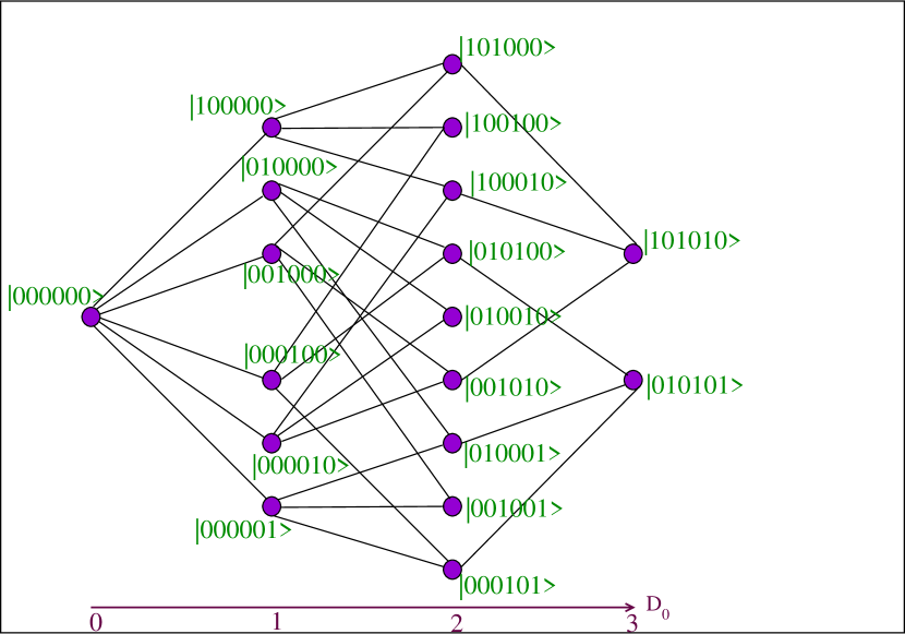
Figure 12: Graph representation of the action of PXP model in the constrained Hilbert space for $L=6$. The Hamming distance ($D_{0}$) of any configuration is measured from the state $|0\rangle$. Here $1~{}(0)\equiv\uparrow(\downarrow)$.

We start from $|v_{0}\rangle=|0\rangle$. We note that $H_{-}|v_{0}\rangle=0$ whereas

$$H^{+}|0\rangle = \sum^{L}_{i=1}\tilde{\sigma}^{+}_{i}|0\rangle=\sum^{L}_{i=1}|\cdots\uparrow_{i}\cdots\rangle=\sum^{L}_{i=1}|i\rangle,$$ (46)

where the ellipsis indicate down spins, and here and in the rest of this Appendix, we shall use the site index (indices) of the up-spin (up-spins) to label a state. In this analysis, we use periodic boundary condition so that the site index is always a number modulo $L$, and $\beta_{1}=\sqrt{||H^{+}|0\rangle||}=\sqrt{L}$. This leads to

$$|v_{1}\rangle=\frac{1}{\beta_{1}}H^{+}|0\rangle=\frac{1}{\sqrt{L}}\sum^{L}_{i=1}|i\rangle.$$ (47)

One can easily check that $H^{-}|v_{1}\rangle=\beta_{1}|v_{0}\rangle$. Thus the action of $H^{+}$ can be totally undone by $H^{-}$ which means that the first FSA step is exact; no error is introduced at this step.

Next, we act $H^{+}$ on $|v_{1}\rangle$ below

$$H^{+}|v_{1}\rangle = \frac{1}{\sqrt{L}}\sum^{L}_{i=1}\tilde{\sigma}^{+}_{i}\sum^{L}_{j=1}|j\rangle$$ (48)

$$= \frac{1}{\sqrt{L}}\sum_{i\neq(j-1),j,(j+1)}\ \sum^{L}_{j=1}|i,j\rangle.$$

The state in Eq. (48) is a superposition of $L(L-3)/2$ distinct two up-spin states. This allows us to write

$$\beta_{2} = \sqrt{||H^{+}|v_{1}\rangle||}=\sqrt{2(L-3)}.$$ (49)

and leads to

$$|v_{2}\rangle = \frac{1}{\beta_{2}}H^{+}|v_{1}\rangle=\sqrt{\frac{2}{L(L-3)}}\sum_{ij}|i,j\rangle,$$ (50)

where the sum is over all distinct two up-spin states in the constrained Hilbert space. Again, we can easily check $H^{-}|v_{2}\rangle=\beta_{2}|v_{1}\rangle$ which means the FSA is exact in the second step.

Next, we act with $H^{+}$ on $|v_{2}\rangle$ which gives

$$H^{+}|v_{2}\rangle=\sqrt{\frac{2}{L(L-3)}}\Big{(}\sum_{i\neq(j-1),j,j+1,j+3}\sum_{j=1}^{L}|i,j,j+2\rangle$$

$$+\sum_{i\neq j,j-1,j+2,j^{\prime}-1,j^{\prime},j^{\prime}+1}\ \sum_{|j^{\prime}-j|\geq 3}\sum_{j=1}^{L}|i,j,j^{\prime}\rangle\Big{)}.$$ (51)

A careful counting of the number of states in Eq. (51) leads to $L(L-4)(L-5)/2$ three-up spin distinct states in Eq. (51) with equal participation. But the total number of distinct three up-spin states in the constrained Hilbert space is $L(L-4)(L-5)/6$. Thus we find

$$\beta_{3}=\sqrt{||H^{+}|v_{2}\rangle||}=\sqrt{\frac{3(L-4)(L-5)}{L-3}},$$ (52)

so that

$$|v_{3}\rangle = \frac{H^{+}|v_{2}\rangle}{\beta_{3}}$$ (53)

$$= \sqrt{\frac{6}{L(L-4)(L-5)}}\sum_{j_{1},j_{2},j_{3}}|j_{1},j_{2},j_{3}\rangle$$

where the sum is taken over all distinct three up-spin states within the constrained Hilbert space. This yields

$$H^{-}|v_{3}\rangle=\sqrt{\frac{6}{L(L-4)(L-5)}}\sum_{j_{1},j_{2}}|j_{1},j_{2}\rangle.$$ (54)

The number of states with two up-spins in Eq. (54) is $L(L-4)(L-5)/2$ which is different from the number of two up-spin states obtained in the second FSA step ($L(L-3)/2$). The ratio of the number of these states is $(L-4)(L-5)/(L-3)$ which is not an integer for all values of $L$. Thus $H^{-}|v_{3}\rangle$ is not proportional to $|v_{2}\rangle$ and the action of $H^{+}$ on $|v_{2}\rangle$ cannot be completely undone by $H^{-}$, i.e., $H^{-}|v_{3}\rangle\neq\beta_{3}|v_{2}\rangle$.

Thus we see that the third FSA step introduces errors; such errors are introduced in all $n\geq 3$ steps. We define the error, $\delta_{n}$, introduced in the $n^{\rm th}$ step as

$$\delta_{n}=||H^{-}|v_{n}\rangle-\beta_{n}|v_{n-1}\rangle||.$$ (55)

In this notation $\delta_{1}=\delta_{2}=0$ and $\delta_{n}\neq 0$ for $n\geq 3$. We note that in the PXP model there is no parameter to tune which may minimize such errors. This indicates the instability of this procedure which becomes more apparent with increasing $L$ where there are more FSA steps. This indicates our need to go beyond the PXP model to find stable $|0\rangle$ scars.

In the next section we show that the inclusion of non-trivial three-spin terms such as the one obtained in ${\rm O}(w^{3})$ perturbation theory in Sec. II of the main text provides a way to minimize such errors.

C.2 FSA in the modified PXP model

In this section we reformulate the FSA by adding a three-spin term similar to that found using Floquet perturbation theory (but with an arbitrary real coefficient $h$) for the bare PXP model. The total Hamiltonian is now

$$H_{1}(h)\equiv H_{1} = \sum_{i=1}^{L}\tilde{\sigma}^{x}_{i}+h\sum_{i=1}^{L}(\tilde{\sigma}^{+}_{i}\tilde{\sigma}^{-}_{i-1}\tilde{\sigma}^{-}_{i+1}+{\rm H.c.}).$$

This can be decomposed in the similar manner as before into $H^{-}_{1}$ and $H^{+}_{1}$, where

$$H^{-}_{1}=\sum_{i=1}^{L}\tilde{\sigma}^{-}_{i}+h\sum_{i=1}^{L}\tilde{\sigma}^{+}_{i}\tilde{\sigma}^{-}_{i-1}\tilde{\sigma}^{-}_{i+1},$$ (57)

and $H^{+}_{1}=(H^{-}_{1})^{\dagger}$. We start again with $|v_{0}\rangle=|0\rangle$. As the additional term in $H_{1}$ annihilates $|0\rangle$, the first FSA step remain unchanged, i.e., $\beta^{n}_{1}=\sqrt{L}$ and $|v^{n}_{1}\rangle=\sum_{i}|i\rangle/\sqrt{L}$.

The second FSA step is more complicated. Here we have

$$H^{+}_{1}|v^{n}_{1}\rangle = \frac{2}{\sqrt{L}}\sum_{i\neq j,j-1,j+1}\sum_{j}|i,j\rangle~{}+~{}\frac{h}{\sqrt{L}}\sum_{i=1}^{L}|i-1,i+1\rangle$$ (58)

$$= \frac{1}{\sqrt{L}}\left[(2+h)\sum_{i=1}^{L}|i-1,i+1\rangle~{}+~{}2\sum_{j\neq(i-2),(i-1),i,(i+1),(i+2)}\ \sum_{i=1}^{L}|i,j\rangle\right].$$

In Eq. (58), the second term on the right represents states with two up-spins that are separated by at least two lattice sites. The norm $\beta^{n}_{2}$ of this state is given by

$$\beta^{n}_{2} = \sqrt{||H^{+}_{1}|v^{n}_{1}\rangle||}=\sqrt{h^{2}+4h+(2L-6)}.$$

This allows us to obtain the new FSA vector in the second step, $|v^{n}_{2}\rangle=H^{+}_{1}|v^{n}_{1}\rangle/\beta_{2}^{n}$. It is possible to check that $H^{-}_{1}|v^{n}_{2}\rangle=\beta_{2}^{n}|v_{1}^{n}\rangle$. This shows that the FSA is error-free up to the second step although the norm and the FSA vectors are modified due to the presence of the three-spin term in $H_{1}$.

We now show that the third FSA step leads to the first non-trivial error. Calculating the action of $H^{+}_{1}$ on $|v_{2}^{n}\rangle$ is straightforward but cumbersome. After grouping all the similar classes of states generated by the action of different terms in $H^{+}_{1}$ and summing the corresponding coefficients, we get

$$H^{+}_{1}|v^{n}_{2}\rangle = \frac{6}{\sqrt{L}\beta^{n}_{2}}\left[\sum_{i=1}^{L}(h+1)|i,i+2,i-2\rangle+(\frac{h}{2}+1)\sum_{j\neq(i-2)..(i+4)}\ \sum_{i=1}^{L}|i,i+2,j\rangle+\sum_{|i-j|\geq 2,|j-k|\geq 2,|i-k|\geq 2}|i,j,k\rangle\right].$$

The last summation in Eq. (LABEL:Hplusnewvnew2) is over those three up-spin states that have no two up-spins as nearest neighbors. The number of such states is $L(L-7)(L-8)/6$. A straightforward calculation, similar to those presented earlier, yields

$$\beta^{n}_{3} = \sqrt{||H^{+}_{1}|v^{n}_{2}\rangle||}$$

$$= \frac{\sqrt{9(L-3)h^{2}+36(L-5)h+6(L-4)(L-5)}}{\beta^{n}_{2}}.$$

Thus we find that the third FSA vector $|v^{n}_{3}\rangle=H^{+}_{1}|v^{n}_{2}\rangle/\beta_{3}^{n}$.

Next we will calculate $H^{-}_{1}|v^{n}_{3}\rangle$. This is straightforward but again involves a complicated counting of states. Here we present the final expression,

$$H^{-}_{1}|v^{n}_{3}\rangle = \frac{1}{\sqrt{L}\beta^{n}_{2}\beta^{n}_{3}}\Big{[}(12(h+1)+3(L-7)(h+2))\sum_{i=1}^{L}|i,i+2\rangle+(12h^{2}+18h+6L-36)\sum_{i=1}^{L}|i,i+3\rangle$$ (62)

$$~{}~{}~{}~{}~{}~{}~{}~{}~{}~{}~{}~{}~{}~{}+(6h^{2}+24h+6L-36)\sum_{j\neq(i-3)..(i+3)}\sum_{i=1}^{L}|i,j\rangle\Big{]}.$$

It is easy to see that $H^{-}_{1}|v^{n}_{3}\rangle\neq\beta^{n}_{3}|v^{n}_{2}\rangle$. The following norm quantifies the error

$$\delta^{n}_{3} = ||H^{-}_{1}|v^{n}_{3}\rangle-\beta^{n}_{3}|v^{n}_{2}\rangle||=\frac{f(h,L)}{g(h,L)},$$

$$f(h,L) = \big{[}(6L+6)h^{6}+(72L-168)h^{5}+(300L-1368)h^{4}+(288L-1608)h^{3}$$ (63)

$$+(30L-438)h^{2}+(-120L+696)h+(24L-120)\big{]},$$

$$g(h,L) = \big{[}(3L-9)h^{4}+(24L-96)h^{3}+(8L^{2}-6L-146)h^{2}+(32L^{2}-264L+520)h+4L^{3}-48L^{2}+188L-240\big{]}.$$

It is easy to see that $\lim_{L\to\infty}\delta^{n}_{3}(h,L)\to 0$ for all $h$ which means that in the thermodynamic limit, the error vanishes. But in a finite system, this error must be minimized to enhance the oscillation from $|0\rangle$. The result of such a minimization is shown in Fig. 13 (a) where $\delta_{3}^{n}$ is plotted as a function of $h$ for $L=50$; we find that it indeed shows a minima at a non-zero $h=h_{3}^{\rm min}$. This points out the importance of the three-spin term in the Hamiltonian; its coefficients provide us with the necessary control knob for minimization of the FSA error leading to maximization of scar-induced oscillations. We note that such a term does not play a similar role for dynamics starting from the $|\mathbb{Z}_{2}\rangle$ state. The minimum value of $\delta_{3}^{n}\equiv\delta^{n\,{\rm min}}_{3}$ as well as the corresponding value of $h_{3}^{\rm min}$ decreases with increasing $L$ as can be seen from Figs. 13 (b) and 13 (c) respectively. We find that $\delta^{n\,{\rm min}}_{3}\to 0$ and $h^{\rm min}\to 0.29$ for sufficiently large but finite $L$.

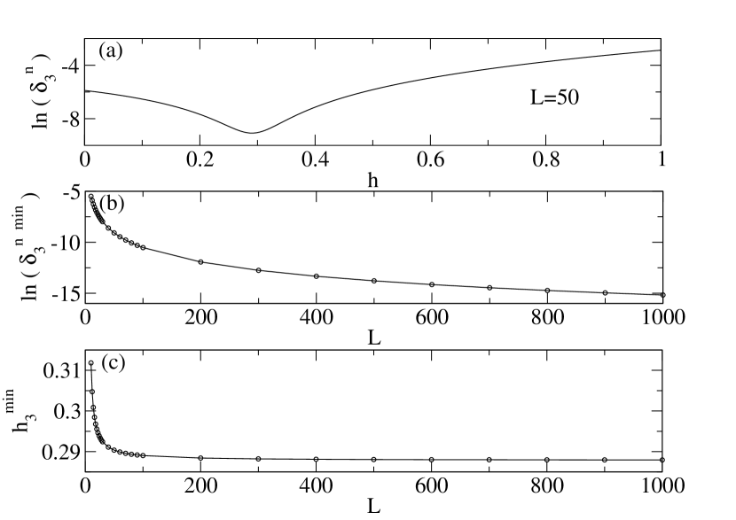
Figure 13: (a) Plot of $\ln(\delta_{3}^{n})$ as a function of $h$ for $L=50$ showing a minima at $h_{3}^{{\rm min}}\simeq 0.3$. (b) Plot of $\ln(\delta^{n\,{\rm min}}_{3})$ as a function of $L$. (c) Plot of $h_{3}^{{\rm min}}$ as a function of $L$ showing its saturation at large $L$.

The above behavior of $\delta_{3}^{n}$ as a function of $h$ and $L$ suggests that the error in further FSA steps will play a crucial role in determining the magnitude of oscillations in the dynamics of the $|0\rangle$ state. However, a systematic analytic study of this seems difficult. We therefore resort to numerical evaluation of these errors denoted by $\delta_{m}^{n}$ for the $m^{\rm th}$ FSA step. The result is shown in Fig. 14 where we plot $\delta_{m}^{n}$ for $m\leq 7$ as a function of $h$ for $L=30$. We find that for all $h$, $\delta_{m}^{n}$ is a monotonically increasing function of $m$. Moreover, they display minima at different values of $h=h_{m}^{\rm min}$ which are close to $h_{3}^{\rm min}=0.31$.

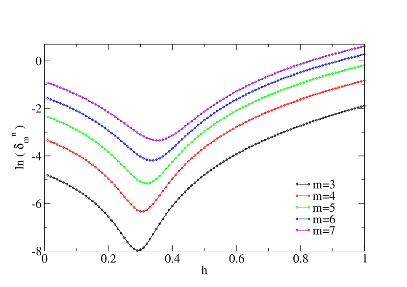
Figure 14: Plot of $\delta_{m}^{n}$ for several FSA steps $m\leq 7$ as a function of $h$ for $L=30$.

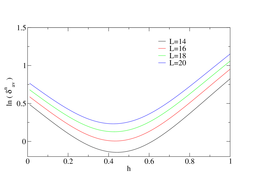
Figure 15: Plot of $\ln\delta^{n}_{\rm av}$ as a function of $h$ for $L=14,16,18,20$.

In Fig. 15 we plot $\ln\delta^{n}_{\rm av}$ as a function of $h$ for several representative values of $L$. Here, the average error is defined as $\delta^{n}_{\rm av}=\sum_{m=3}^{L/2}\delta^{n}_{m}/((L/2)-2)$. The plot indicates that tuning of $h$ can minimize the average (and hence the total) error. However, the average error is a monotically increasing function of $L$. This indicates decrease of DE (and hence the oscillaion amplitude) value with $L$ in the superthermal phase as mentioned in the main text.

Next, we explore the possibility of maximizing the scar-induced oscillations in these systems by allowing higher spin terms cai . These terms have support over $(2m+3)$ sites for a $(2m+1)$-spin term. Here, we shall concentrate on the lowest such term so that the Hamiltonian is

$$H_{2} = H_{1}[h_{3}]+h_{5}\sum_{j}(\tilde{\sigma}_{j-1}^{+}\tilde{\sigma}_{j+1}^{+}\tilde{\sigma}^{-}_{j+2}\tilde{\sigma}_{j}^{-}\tilde{\sigma}_{j-2}^{-}+{\rm H.c.}),$$

such that the five-spin term has support over seven consecutive sites. We note that it is experimentally challenging to generate such terms with high enough amplitude; however, they are automatically generated, albeit with lower strength, in our driven system for the periodic protocol studied in this work. The aim of our analysis here is to demonstrate that these terms indeed lead to oscillations starting from the $|0\rangle$ state and that such oscillations can be maximized by tuning their strength.

To this end, we now repeat our analysis detailed out earlier using $H_{2}$. Since our aim is to maximize the oscillation amplitude of $O_{22}(n)$, we first numerically find the combination $\vec{h}^{\rm max}=(h_{3}^{\rm max},h_{5}^{\rm max})$ which maximizes the DE value of $O_{22}$; these values maximize the oscillation amplitude as shown in Fig. 16 for $L=14$ where the initial state $|0\rangle$ is propagated in time using $H_{2}$. We find that $\vec{h}^{\rm max}=(0.43,0,28)$. From Fig. 16, it is clear that the oscillations in $O_{22}$ decrease when the $h_{5}$ term is set to zero and $h_{3}$ is then set to its optimum value, while the bare PXP Hamiltonian (setting both $h_{3}$ and $h_{5}$ to be zero) gives still weaker oscillations.

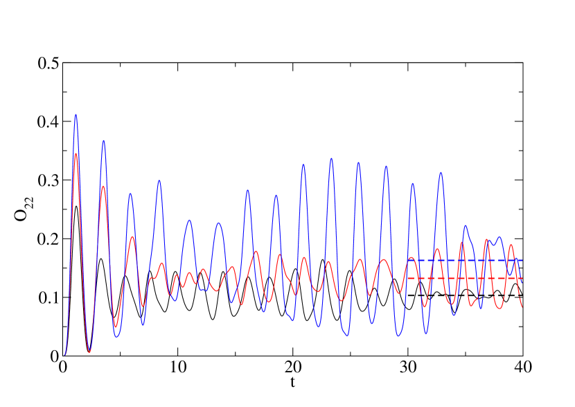
Figure 16: Plots of $O_{22}$ as a function of $t$ starting from $|0\rangle$ with the bare PXP Hamiltonian (black solid line), $H_{1}$ with $h=0.31$ (red solid line), and $H_{2}$ with $\vec{h}=(0.43,0.28)$ (blue solid line). The corresponding diagonal ensemble values are denoted by the dashed lines. For all plots, the system size equals $L=14$ and $t$ is measured in units of $w^{-1}$

.

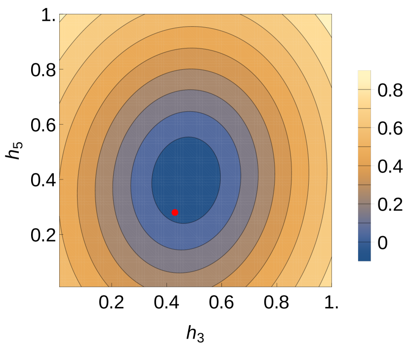
Figure 17: Plot of $\ln\delta_{\rm av}^{n}$ as a function of $h_{3}$ and $h_{5}$ for $L=14$. The red dot indicates the position of $\vec{h}^{\rm max}$.

Next, we carry out the FSA analysis using $H_{2}$ and starting from the $|0\rangle$ state. Here we find that most of the features of errors generated in different FSA steps mimics our earlier analysis. In particular, we find that the FSA error at the $m^{\rm th}$ step $\delta_{m}$ is minimized for different values of $\vec{h}$; there is no value of $\vec{h}$ which minimizes all FSA errors. We therefore choose to minimize $\delta_{\rm av}^{n}$. A plot of $\ln\delta_{\rm av}^{n}$ as a function of $h_{3}$ and $h_{5}$ is shown in Fig. 17; this yields $\vec{h}^{\rm min}=(0.45,0.4)$. The red dot in Fig. 17 indicates $\vec{h}^{\rm max}$. We note that $\vec{h}_{3}^{\rm min}$ is close to $\vec{h}_{3}^{\rm max}$ obtained earlier. However, the value $\vec{h}^{\rm min}$ depends on our choice of minimization parameter; for example, minimization of errors of a specific step (say $\delta_{5}^{n}$ or $\delta_{6}^{n}$) or the geometric mean of errors $(\prod_{m=3,7}\delta_{m}^{n})^{1/5}$ would leads to $\vec{h}^{\rm min}$ almost identical to $\vec{h}^{\rm max}$. We leave a more detailed analysis of this issue as a subject of future work.

References

- (1) M. Greiner, O. Mandel, T. Esslinger, T. W. Hansch, and I. Bloch, Nature 39, 415 (2002).
- (2) I. Bloch, J. Dalibard, and W. Zwerger, Rev. Mod. Phys. 80, 885 (2008).
- (3) J. Simon, W. S. Bakr, R. Ma, M. E. Tai, P. M. Preiss, and M. Greiner, Nature (London) 472, 307 (2011); W. Bakr, A. Peng, E. Tai, R. Ma, J. Simon, J. Gillen, S. Foelling, L. Pollet, and M. Greiner, Science 329, 547 (2010).
- (4) H. Bernien, S. Schwartz, A. Keesling, H. Levine, A. Omran, H. Pichler, S. Choi, A. S. Zibrov, M. Endres, M. Greiner, V. Vuletic, and M. D. Lukin, Nature 551, 579 (2017).
- (5) S. Sachdev, K. Sengupta, and S. M. Girvin, Phys. Rev. B 66, 075128 (2002).
- (6) S. Pielawa, T. Kitagawa, E. Berg, and S. Sachdev, Phys. Rev. B 83, 205135 (2011).
- (7) J. Dziarmaga, Adv. Phys. 59, 1063 (2010).
- (8) A. Polkovnikov, K., Sengupta, A. Silva, A. and M. Vengalattore, Rev. Mod. Phys. 83, 863 (2011).
- (9) A. Dutta, G. Aeppli, B. K. Chakrabarti, U. Divakaran, T. F. Rosenbaum, and D. Sen, Quantum Phase Transitions in Transverse Field Spin Models: From Statistical Physics to Quantum Information (Cambridge University Press, Cambridge, 2015).
- (10) S. Mondal, D. Sen, and K. Sengupta, Quantum Quenching, Annealing and Computation, edited by Das, A., Chandra, A. & Chakrabarti, B. K. Lecture Notes in Physics, Vol. 802 (Springer, Berlin, Heidelberg, 2010), Chap. 2, p. 21.
- (11) L. D’Alessio, Y. Kafri, A. Polkovnikov, and M. Rigol, Adv. Phys. 65, 239 (2016).
- (12) J. M. Deutsch, Phys. Rev. A 43, 2046 (1991).
- (13) M. Srednicki, Phys. Rev. E 50, 888 (1994); ibid, J. Phys. A 32, 1163 (1999).
- (14) M. Rigol, V. Dunjko, and M. Olshanii, Nature (London) 452, 854 (2008).
- (15) M. Basko, I. L. Aleiner, and B. L. Altshuler, Ann. Phys. 321, 1126 (2006).
- (16) R. Nandkishore and D. Huse, Ann. Rev. Cond. Mat. 6, 15 (2015).
- (17) E. J. Heller, Phys. Rev. Lett. 53, 1515 (1984).
- (18) S. Choi, C. J. Turner, H. Pichler, W. W. Ho, A. A. Michailidis, Z. Papić, M. Serbyn, M. D. Lukin, and D. A. Abanin, Phys. Rev. Lett. 122, 220603 (2019).
- (19) W. W. Ho, S. Choi, H. Pitchler, and M. D. Lukin, Phys. Rev. Lett. 122, 040603 (2019).
- (20) C. J. Turner, A. A. Michailidis, D. A. Abanin, M. Serbyn, and Z. Papić, Nat. Phys. 14, 745 (2018).
- (21) C. J. Turner, A. A. Michailidis, D. A. Abanin, M. Serbyn, and Z. Papić, Phys. Rev. B 98, 155134 (2018).
- (22) K. Bull, I. Martin, and Z. Papić, Phys. Rev. Lett. 123, 030601 (2019).
- (23) V. Khemani, C. R. Lauman, and A. Chandran, Phys. Rev. B99, 161101 (2019).
- (24) S. Maudgalya, N. Regnault, and B. A. Bernevig, Phys. Rev. B98, 235156 (2018).
- (25) T. Iadecola, M. Schecter, and S. Xu, Phys. Rev. B 100, 184312 (2019).
- (26) N. Shiraishi, J. Stat. Mech. 08313 (2019).
- (27) M. Schecter, and T. Iadecola, Phys. Rev. Lett. 123, 147201 (2019).
- (28) B. Mukherjee, S. Nandy, A. Sen, D. Sen, and K. Sengupta, arXiv:1907.08212 (unpublished).
- (29) B. Mukherjee, A. Sen, D. Sen, and K. Sengupta, arXiv:2002.08683 (unpublished).
- (30) A. Soori and D. Sen, Phys. Rev. B 82, 115432 (2010); A. Haldar, D. Sen, R. Moessner, and A. Das, arXiv:1909.04064 (unpublished).
- (31) T. Bilitewski and N. Cooper, Phys. Rev A 91, 063611 (2015).
- (32) A. Das, Phys. Rev. B82, 172402 (2010); S. Bhattacharyya, A. Das, and S. Dasgupta, Phys. Rev. B86, 054410 (2012); S. S. Hedge, H. Katiyar, T. S. Mahesh, and A. Das, Phys. Rev. B90, 174407 (2014).
- (33) S. Mondal, D. Pekker, and K. Sengupta, Europhys. Lett. 100, 60007 (2012); U. Divakaran and K. Sengupta, Phys. Rev. B90, 184303 (2014); S. Kar, B. Mukherjee, and K. Sengupta, Phys. Rev. B94, 075130 (2016); S. Lubini, L. Chirondojan, G. Oppo, A. Politi, and P. Politi, Phys. Rev. Lett. 122, 084102 (2019).
- (34) P. Reimann, Phys. Rev. Lett. 101, 190403 (2008).
- (35) S. Vajnam, K. Klobas, T. Prosen, and A. Polkovnikov, Phys. Rev. Lett. 120, 200607 (2018).
- (36) T. Kuwahara, T. Mori, and K. Saito, Annals of Physics 367, 96 (2016).
- (37) Y. Chen and Z. Cai , Phys. Rev. A 101, 023611 (2020).