A solution to the overdamping problem when simulating dust-gas mixtures with smoothed particle hydrodynamics

Abstract

We present a fix to the overdamping problem found by Laibe & Price (2012) when simulating strongly coupled dust-gas mixtures using two different sets of particles using smoothed particle hydrodynamics. Our solution is to compute the drag at the barycentre between gas and dust particle pairs when computing the drag force by reconstructing the velocity field, similar to the procedure in Godunov-type solvers. This fixes the overdamping problem at negligible computational cost, but with additional memory required to store velocity derivatives. We employ slope limiters to avoid spurious oscillations at shocks, finding the van Leer Monotonized Central limiter most effective.

1 Introduction

In Laibe & Price (2012a, b) (hereafter LP12a,b) we found three problems when using Lagrangian particles to simulate the dust component of dust-gas mixtures: i) artificial trapping of dust particles below the gas resolution, ii) overdamping of waves and slow convergence at high drag, requiring prohibitive spatial resolution iii) timestepping, requiring timesteps shorter than the stopping time, or an implicit scheme (e.g. Monaghan, 1997; Miniati, 2010; Bai & Stone, 2010; Lorén-Aguilar & Bate, 2014; Yang & Johansen, 2016; Stoyanovskaya et al., 2018; Monaghan, 2020).

In our 2012 study, using smoothed particle hydrodynamics (SPH; Monaghan 1992), we found our numerical solutions for linear waves to be over-damped compared to the analytic solution when the drag between dust and gas was high, i.e., for small grains. Miniati (2010) similarly found only first order accuracy in the stiff regime when simulating dust as particles and gas on a grid (see also Yang & Johansen 2016). This is the ‘overdamping problem’.

In Laibe & Price 2014a, b we solved this problem by re-writing the dust/gas equations to describe a single fluid mixture (i.e. as a single set of SPH particles with an evolving dust fraction). This approach avoids the overdamping problem but the mixture approach is only suitable for small grains. Stoyanovskaya et al. (2018) showed that overdamping could be avoided even with dust and gas as particles by interpolating the dust and gas velocities to a common spatial position. Our approach is based on a similar idea.

In this paper we show that the overdamping problem in SPH can be solved by applying ideas from Finite Volume codes, namely reconstruction of the velocity field between pairs of gas and dust particles.

2 Methods

2.1 Continuum equations

Consider a gas and dust mixture represented by two different types of particles. The momentum and energy equations are

$$\frac{\partial\bm{v}_{\rm g}}{\partial t}+(\bm{v}_{\rm g}\cdot\nabla)\bm{v}_{\rm g} =-\frac{\nabla P_{\rm g}}{\rho_{\rm g}}+\frac{K}{\rho_{\rm g}}(\bm{v}_{\rm d}-\bm{v}_{\rm g}),$$ (1)

$$\frac{\partial\bm{v}_{\rm d}}{\partial t}+(\bm{v}_{\rm d}\cdot\nabla)\bm{v}_{\rm d} =-\frac{K}{\rho_{\rm d}}(\bm{v}_{\rm d}-\bm{v}_{\rm g}),$$ (2)

$$\frac{\partial u_{\rm g}}{\partial t}+(\bm{v}_{\rm g}\cdot\nabla)u_{\rm g} =-\frac{P_{\rm g}}{\rho_{\rm g}}(\nabla\cdot\bm{v}_{\rm g})+\frac{K}{\rho_{\rm g}}(\bm{v}_{\rm d}-\bm{v}_{\rm g})^{2}.$$ (3)

2.2 SPH equations

Our SPH algorithm follows LP12a,b in everything except the discrete form of the drag terms. We replace these with

$$\left.\frac{{\rm d}\bm{v}_{a}}{{\rm d}t}\right|_{\rm drag}= +\nu\sum_{i}\frac{m_{i}}{(\rho_{i}+\rho_{a})t^{ai}_{\rm s}}\left(\bm{v}^{*}_{ai}\cdot\hat{\bm{r}}_{ai}\right)\hat{\bm{r}}_{ai}D_{ai}(h),$$ (4)

$$\left.\frac{{\rm d}\bm{v}_{i}}{{\rm d}t}\right|_{\rm drag}= -\nu\sum_{a}\frac{m_{a}}{(\rho_{a}+\rho_{i})t^{ai}_{\rm s}}\left(\bm{v}^{*}_{ai}\cdot\hat{\bm{r}}_{ai}\right)\hat{\bm{r}}_{ai}D_{ai}(h),$$ (5)

$$\left.\frac{{\rm d}u_{a}}{{\rm d}t}\right|_{\rm drag}= \nu\sum_{i}\frac{m_{i}}{(\rho_{a}+\rho_{i})t^{ai}_{\rm s}}\left(\bm{v}^{*}_{ai}\cdot\hat{\bm{r}}_{ai}\right)\left(\bm{v}_{ai}\cdot\hat{\bm{r}}_{ai}\right)D_{ai}(h),$$ (6)

where the index $a$ refers to gas particles while $i$ refers to dust particles, $\nu$ is the number of dimensions, $\bm{v}_{ai}\equiv\bm{v}_{a}-\bm{v}_{i}$, $\bm{r}_{ai}\equiv\bm{r}_{a}-\bm{r}_{i}$, $D_{ai}(h)\equiv D(|\bm{r}_{ai}|,\max[h_{a},h_{i}])$ is a double-humped kernel (LP12a), and the stopping time is defined via

$$t_{\rm s}^{ai}\equiv\frac{\rho_{a}\rho_{i}}{K(\rho_{a}+\rho_{i})},$$ (7)

where density is only computed using neighbours of the same type (i.e. gas density on gas particles and dust density on dust particles). Here we assume $K$ constant, but in general $t_{\rm s}$ may be set according to a physical drag law e.g. Epstein drag. The only difference in our formulation of the drag terms compared to LP12a is that we use a reconstructed velocity for the interaction between particle pairs denoted $\bm{v}^{*}$, rather than the velocity at the position of the particle itself. This improves the estimate of the local differential velocity.

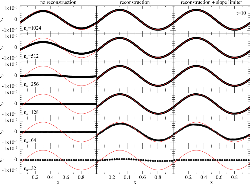
Figure 1: Dust and gas velocities in the dustywave test after 10 wave periods, using $K=1000$ with $2\times n_{x}$ particles without reconstruction and with and without the slope limiter (see labels). Reconstruction avoids the need to resolve $h\sim t_{\rm s}c_{\rm s}$ (resolved at $n_{x}=1024$ particles). Exact solution shown in red.

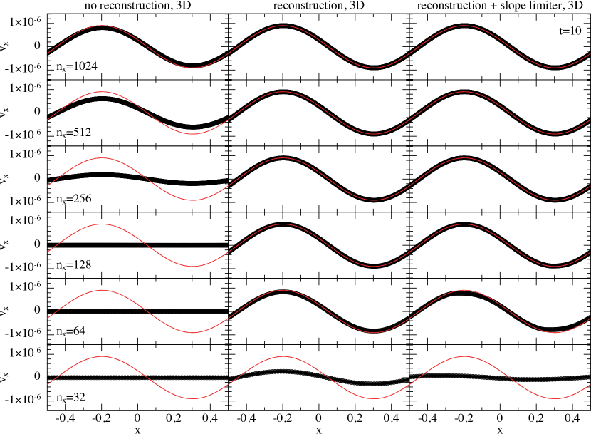
Figure 2: As in Figure 1 but in 3D with phantom using $n_{x}\times 12\times 12$ gas particles (solid) and $n_{x}\times 12\times 12$ dust particles (open) initially placed using dense sphere packing. Exact solution from Laibe & Price (2011) shown in red.

2.3 Reconstruction

We reconstruct the velocity for each particle pair ($a$,$i$) using

$$\bm{v}^{*}_{a} =\bm{v}_{a}+\left(\bm{r}^{*}-\bm{r}_{a}\right)^{\beta}\frac{\partial\bm{v}_{a}}{\partial\bm{r}_{a}^{\beta}};$$ (8)

$$\bm{v}^{*}_{i} =\bm{v}_{i}+\left(\bm{r}^{*}-\bm{r}_{i}\right)^{\beta}\frac{\partial\bm{v}_{i}}{\partial\bm{r}_{i}^{\beta}}.$$ (9)

where to avoid confusion with particle labels we use $\alpha$, $\beta$ and $\gamma$ to refer to tensor indices, with repeated tensor indices implying summation. At the barycentre between the particles $a$ and $i$ — i.e., at $\bm{r}^{*}=\bm{r}_{a}+\mu_{ai}\bm{r}_{ai}=\bm{r}_{i}-\mu_{ia}\bm{r}_{ai}$, these relations combine to

$$\bm{v}^{*}_{ai}\cdot\hat{\bm{r}}_{ai}=\bm{v}_{ai}\cdot\hat{\bm{r}}_{ai}-\mu_{ai}|r_{ai}|\left(S_{ai}+S_{ia}\right),$$ (10)

where $S_{ai}\equiv\hat{r}_{ai}^{\alpha}\hat{r}_{ai}^{\beta}\frac{\partial v_{a}^{\alpha}}{\partial x_{a}^{\beta}}$ and $\mu_{ai}=m_{a}/\left(m_{a}+m_{i}\right)$. Velocity gradients are computed using an exact linear derivative operator (e.g. Price, 2012), i.e. by solving the $3\times 3$ matrix equation

$$R_{\beta\gamma}\frac{\partial v^{\alpha}}{\partial r^{\gamma}}=-\sum_{b}m_{b}v^{\alpha}_{ab}\nabla^{\beta}W_{ab}\left(h_{a}\right),$$ (11)

where

$$R_{\beta\gamma}=\sum_{b}m_{b}(\bm{r}_{b}-\bm{r}_{a})^{\beta}\nabla^{\gamma}W_{ab}(h_{a}).$$ (12)

The summations on the right hand side of Equations 11 and 12 are computed during the density summation, with the summation index over particles of the same type. We found no difference using the exact linear operator versus the usual SPH derivative.

2.4 Slope limiters

The danger with reconstruction is the reintroduction of spurious oscillations when the solution is discontinuous. To prevent this, the factor $\left(S_{ai}+S_{ia}\right)$ may be replaced by a slope limiter, i.e. a function $2f\left(S_{ai},S_{ia}\right)$ that preserves monotonicity (van Leer, 1974). We explored a range of limiters (e.g. Sweby 1984) including, from most to least dissipative, minmod

$$f(a,b)=\begin{cases}\min(|a|,|b|)&a>0,b>0\\ -\min(|a|,|b|)&a<0,b<0\\ 0&\text{otherwise},\end{cases}$$ (13)

van Leer (van Leer, 1977)

$$f(a,b)=\begin{cases}\frac{2ab}{a+b}&ab>0\\ 0&\text{otherwise},\end{cases}$$ (14)

van Leer Monotonized Central (MC) (van Leer, 1977)

$$f(a,b)=\begin{cases}\text{sgn}(a)\min(|\frac{1}{2}(a+b)|,2|a|,2|b|)&ab>0\\ 0&\text{otherwise},\end{cases}$$ (15)

and Superbee (Roe, 1986; Sweby, 1984)

$$f(a,b)=\begin{cases}\text{sgn}(a)\max\left[\min(|b|,2|a|),\min(2|b|,|a|)\right]&ab>0\\ 0&\text{otherwise}.\end{cases}$$ (16)

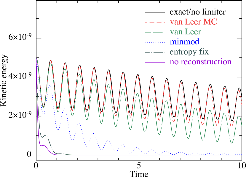
Figure 3: Kinetic energy as a function of time in the 1D dustywave problem, comparing different slope limiters. From top to bottom results employ reconstruction with no limiter, the van Leer MC, van Leer and minmod limiters, our ‘entropy fix’ (Section 2.5), and no reconstruction.

Figure 4: Convergence on the dustywave problem, showing $L_{1}$ error as a function of the number of particles per wavelength in 1D. Solid line uses reconstruction and the van Leer MC limiter, dashed line no reconstruction. Dotted line shows slope of $-2$ expected for 2nd order. Arrow indicates the no-longer-necessary $h\lesssim c_{\rm s}t_{\rm s}$ criterion required by LP12a.

2.5 Slope limiters and entropy

Slope limiters are usually employed in the context of Total Variation Diminishing (TVD) schemes (Harten, 1983), but application of the TVD concept beyond 1D or to unstructured/meshfree methods is less clear (e.g. Chiapolino, Saurel & Nkonga 2017). A physical interpretation can be seen from our Equation 6. For the drag term to provide a positive definite contribution to the entropy $\bm{v}_{ai}\cdot\hat{\bm{r}}_{ai}$ and $\bm{v}^{*}_{ai}\cdot\hat{\bm{r}}_{ai}$ must have the same sign, such that ${\rm d}u/{\rm d}t|_{\rm drag}$ is positive. Pairwise positivity is not strictly necessary so long as the sum over all neighbours is positive. We tried setting $\bm{v}^{*}_{ai}\cdot\hat{\bm{r}}_{ai}=\bm{v}_{ai}\cdot\hat{\bm{r}}_{ai}$ if the signs differ, but found this to be more dissipative than using slope limiters (see Figure 3). We found the van Leer MC limiter to provide the best compromise between monotonicity and dissipation.

3 Results

We test our improved algorithm in 1D using the ndspmhd code (Price, 2012) and in 3D using phantom (Price et al., 2018). We use explicit global timestepping with a leapfrog integrator, the M₆ quintic kernel for the SPH terms with the double hump M₆ employed for the drag terms (LP12a). The results are not sensitive to the choice of kernel provided a double hump kernel is used for the drag. The timestep was set to 0.9 times the minimum stopping time (we found that setting $\Delta t=t_{\rm s}$ exactly as in LP12a could result in instability with reconstruction). We use the van Leer MC limiter unless otherwise specified.

3.1 Dustywave

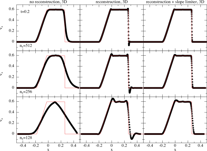
Figure 5: Results of the dustyshock problem performed in 3D with phantom, performed at three different numerical resolutions (bottom to top) with no reconstruction (left column), with reconstruction but no slope limiter (middle) and using reconstruction with the van Leer MC limiter (right column). Exact solution in red, points show velocity on gas (solid) and dust (open circles) particles.

Figure 1 shows the results of the dustywave described in Laibe & Price (2011), performed using $2\times n_{x}$ particles with a fixed drag coefficient $K=1000$, $\rho_{\rm g}=\rho_{\rm d}=1$ and $c_{\rm s}=1$ (giving $t_{\rm s}=5\times 10^{-4}$) and a perturbation amplitude of $10^{-6}$. We use an adiabatic equation of state $P=(\gamma-1)\rho u$ with $\gamma=5/3$ in the gas. In the absence of reconstruction, overdamping occurs when $h\gtrsim c_{\rm s}t_{\rm s}$, i.e. for $n_{x}\lesssim 1024$ (left column), as found by LP12a. Adding reconstruction captures the true solution to within a few percent for $n_{x}\gtrsim 64$ (middle column), while the slope limiter does not visibly degrade it (right column).

Figure 2 shows the results in 3D using phantom. We follow the procedure used in Price et al. (2018), placing the particles using dense sphere packing and cropping the grid in the $y$ and $z$ directions at 12 particle spacings (for efficiency), giving $2\times 128\times 12\times 12$ particles. The results in 3D are indistinguishable from those shown in Figure 1, showing our method also works in three dimensions.

3.1.1 Choice of slope limiter

Figure 3 shows the kinetic energy as a function of time in the 1D dustywave problem at a resolution of $n_{x}=128$. The solution with reconstruction but no slope limiter (solid black line) is indistinguishable from the analytic damping rate (Laibe & Price, 2011). By contrast, the solution with no reconstruction (magenta line) is damped in less than one wave period. All limiters apart from Superbee (not shown) give results intermediate between these two extremes. Superbee, defined as the least dissipative limiter to satisfy the TVD property (Sweby, 1984), was found to increase rather than decrease the kinetic energy and produce a clipped wavefront. This numerical ‘over-steepening’ is a known problem with Superbee (e.g. Klee et al., 2017). The Van Leer MC limiter gives the closest match to the analytic damping rate while still remaining effective at shocks (see below). More dissipative limiters all bring back some degree of overdamping. No limiter apart from our entropy fix was found to guarantee positive entropy.

3.1.2 Convergence

Figure 4 shows the $L_{1}$ error $(1/N\sum|v_{x}-v_{x,{\rm exact}}|)$ as a function of the number of particles per wavelength for the 1D dustywave problem. Without reconstruction convergence is flat at low resolution $(n_{x}\leq 256$) because the wave is almost completely damped, becoming second order only after the $h<c_{\rm s}t_{\rm s}$ criterion is satisfied ($n_{x}\gtrsim 1000$). With reconstruction and the slope limiter we find second order convergence for $n_{x}\gtrsim 32$, once the wave is sufficiently resolved for gradients to be accurate.

3.2 Dustyshock

Figure 5 shows the results of the dustyshock test from LP12a at three different numerical resolutions (bottom to top). Lehmann & Wardle (2018) also proposed a dusty shock test, but their test is for the intermediate regime where the drag is moderate. Here we are interested in the strong drag regime, where the stopping time is negligible.

We set up the problem as usual with gas with $x<0$ set up with $(\rho,P,v_{x})=(1.0,1.0,0.0)$ and gas with $x>=0$ set up with $(\rho,P,v_{x})=(0.125,0.1,0.0)$. We performed the test in both 1D and 3D but only show results from the 3D calculation since, as for the wave test, they are very similar to those obtained in 1D. In 3D we set the particle spacing using $n_{x}\times n_{y}\times n_{z}$ gas particles for $x\in[-0.5,0.0]$, and $n_{x}/2\times n_{y}/2\times n_{z}/2$ gas particles in $x\in[0.0,0.5]$ to resolve the 8:1 density contrast without introducing highly anisotropic initial particle distributions. As for the wave test we crop the domain in the $y$ and $z$ directions to match the particle spacing, using $n_{y}=24$ and $n_{z}=24$. We initialise the dust as copies of the gas particles, assuming a dust-to-gas ratio of unity. We apply artificial viscosity as usual using the modified version of the Cullen & Dehnen 2010 switch (see Price et al. 2018 for details).

Figure 5 shows results using the default approach (left column), which at low resolution (bottom left panel) produces a solution appropriate for a smaller drag coefficient. Applying reconstruction with no slope limiter (middle column) the numerical solution is much closer to the exact solution (red line), resolves shock discontinuities to within $\sim 3h$, but produces an unphysical oscillation ahead of the shock front. The right column shows that the slope limiter eliminates such oscillations.The remaining defects in the solution (e.g. at $x=-0.02$) can be seen to disappear as the numerical resolution is increased (right column, bottom to top), with the corresponding $L_{1}$ error reducing from $1.4\times 10^{-2}$ at $n_{x}=128$ to $6.6\times 10^{-3}$ using $n_{x}=256$ and $4.0\times 10^{-3}$ using $n_{x}=512$.

We employed $n_{x}=11,255$ particles in 1D to obtain reasonable results on this problem in LP12a!

4 Discussion

In this paper we have shown how the overdamping problem can be fixed by evaluating the drag at the barycentre of each dust-gas particle pair. The slow convergence observed by LP12a is caused by the particle separation (of order the resolution length, $h$) being too large to correctly resolve the drag lengthscale $l\sim c_{\rm s}t_{\rm s}$. This is why the issue is absent when simulating the dust and gas as a single fluid mixture (Laibe & Price, 2014a, b). A similar idea of interpolating the velocities to a common spatial position was also employed by Stoyanovskaya et al. (2018) as part of their implicit scheme, where it was also shown to solve the overdamping problem. We used explicit timestepping and employed slope limiters to avoid introducing unphysical oscillations at shock fronts. Fung & Muley (2019) similarly found reconstruction of the velocity field necessary for accurate drag in their semi-analytic hybrid (dust as particles, gas on the grid) scheme.

Solving the overdamping problem does not make the other problems go away. Timestepping is relatively easy to solve, with numerous implicit methods already proposed both in the context of SPH (Monaghan, 1997; Laibe & Price, 2012b; Lorén-Aguilar & Bate, 2014, 2015; Stoyanovskaya et al., 2018; Monaghan, 2020) and in Eulerian particle-gas codes (e.g. Miniati, 2010; Bai & Stone, 2010; Yang & Johansen, 2016; Fung & Muley, 2019). Our work makes these worth implementing, since overdamping remains with implicit time integration (see Figures 6–9 of Lorén-Aguilar & Bate 2014). That is, although these schemes make calculation of small grain species efficient, in the absence of our fix they remain inaccurate at high drag. Lorén-Aguilar & Bate 2014 showed that the overdamping was not as severe when the dust-to-gas ratio is low, which suggests a modified criterion $h<c_{\rm s}t_{\rm s}/\epsilon$. With reconstruction or interpolation no spatial resolution criterion is necessary, as found by Stoyanovskaya et al. (2018).

The artificial trapping problem is harder to solve. A single fluid model with no approximations (Laibe & Price, 2014a) can accurately capture waves and shocks for both small and large grains with no artificial trapping (Laibe & Price, 2014b; Benítez-Llambay et al., 2019). However, a single fluid model fails to capture large grains with significant inertia because the dust velocity field is assumed to be single valued everywhere, meaning that dust particles cannot stream or interpenetrate (Laibe & Price, 2014b). The domain of validity is thus reduced in any case to the regime of small grains, where the terminal velocity approximation greatly simplifies matters (Laibe & Price, 2014a; Price & Laibe, 2015; Ballabio et al., 2018). The single fluid method has been extended to multiple grain species (Hutchison et al., 2018; Benítez-Llambay et al., 2019; Lebreuilly et al., 2019). But for large grains one is forced to use particles. Our approach to avoid artificial trapping to date has been to over-resolve the gas compared to the dust (e.g. Mentiplay et al., 2019). This works but is not fail-safe. Artificial trapping also occurs with tracer particles in Eulerian simulations (e.g. Price & Federrath, 2010), where Cadiou et al. (2019) proposed the ‘Monte Carlo tracer particle’ method as a solution. Whether or not similar ideas could be applied to dust-gas mixtures would be worth investigating.

An obvious extension of our method is to apply the same principles to shock capturing in SPH, by using reconstruction in the artificial viscosity terms. We have published preliminary experiments in a conference proceedings (Price, 2019). Rosswog (2019) has also recently proposed a similar method, using both first and second derivatives in the reconstruction.

The main caveat, which would also apply to shock capturing, is that the entropy increase is not guaranteed to be positive definite. While we found the errors to be small, it would be desirable to guarantee positivity while eliminating overdamping.

5 Conclusions

We have shown how the overdamping problem when simulating dust-gas mixtures with separate sets of particles in SPH can be solved by ‘reconstructing’ the velocity field between pairs of dust and gas particles using an approach similar to that employed in finite volume schemes. A slope limiter is needed to avoid oscillations at shocks. The advantange of the new method is that the overdamping problem can be solved with minor changes to existing dust-gas SPH codes at negligible computational expense. The disadvantages are that performing reconstruction requires storage of nine velocity derivatives per particle and does not always guarantee positive entropy despite our use of slope limiters. Our algorithm is implemented in the public phantom code (Price et al., 2018).

References

- Bai & Stone (2010) Bai X.-N., Stone J. M., 2010, ApJS, 190, 297
- Ballabio et al. (2018) Ballabio G., et al., 2018, MNRAS, 477, 2766
- Benítez-Llambay et al. (2019) Benítez-Llambay P., Krapp L., Pessah M. E., 2019, ApJS, 241, 25
- Cadiou et al. (2019) Cadiou C., Dubois Y., Pichon C., 2019, A&A, 621, A96
- Chiapolino et al. (2017) Chiapolino A., Saurel R., Nkonga B., 2017, J. Comp. Phys., 340, 389
- Cullen & Dehnen (2010) Cullen L., Dehnen W., 2010, MNRAS, 408, 669
- Fung & Muley (2019) Fung J., Muley D., 2019, ApJS, 244, 42
- Harten (1983) Harten A., 1983, J. Comp. Phys., 49, 357
- Hutchison et al. (2018) Hutchison M., Price D. J., Laibe G., 2018, MNRAS, 476, 2186
- Klee et al. (2017) Klee J., Illenseer T. F., Jung M., Duschl W. J., 2017, A&A, 606, A70
- Laibe & Price (2011) Laibe G., Price D. J., 2011, MNRAS, 418, 1491
- Laibe & Price (2012a) Laibe G., Price D. J., 2012a, MNRAS, 420, 2345
- Laibe & Price (2012b) Laibe G., Price D. J., 2012b, MNRAS, 420, 2365
- Laibe & Price (2014a) Laibe G., Price D. J., 2014a, MNRAS, 440, 2136
- Laibe & Price (2014b) Laibe G., Price D. J., 2014b, MNRAS, 440, 2147
- Lebreuilly et al. (2019) Lebreuilly U., Commerçon B., Laibe G., 2019, A&A, 626, A96
- Lehmann & Wardle (2018) Lehmann A., Wardle M., 2018, MNRAS, 476, 3185
- Lorén-Aguilar & Bate (2014) Lorén-Aguilar P., Bate M. R., 2014, MNRAS, 443, 927
- Lorén-Aguilar & Bate (2015) Lorén-Aguilar P., Bate M. R., 2015, MNRAS, 454, 4114
- Mentiplay et al. (2019) Mentiplay D., Price D. J., Pinte C., 2019, MNRAS, 484, L130
- Miniati (2010) Miniati F., 2010, J. Comp. Phys., 229, 3916
- Monaghan (1992) Monaghan J. J., 1992, ARA&A, 30, 543
- Monaghan (1997) Monaghan J., 1997, J. Comp. Phys., 138, 801
- Monaghan (2020) Monaghan J. J., 2020, European Journal of Mechanics B Fluids, 79, 454
- Price (2007) Price D. J., 2007, PASA, 24, 159
- Price (2012) Price D. J., 2012, J. Comp. Phys., 231, 759
- Price (2019) Price D. J., 2019, in Lorén-Aguilar P., ed., 14th SPHERIC International Workshop 25-27 June 2019. University of Exeter, Exeter, UK
- Price & Federrath (2010) Price D. J., Federrath C., 2010, MNRAS, 406, 1659
- Price & Laibe (2015) Price D. J., Laibe G., 2015, MNRAS, 451, 5332
- Price et al. (2018) Price D. J., et al., 2018, PASA, 35, e031
- Roe (1986) Roe P. L., 1986, Annual Review of Fluid Mechanics, 18, 337
- Rosswog (2019) Rosswog S., 2019, arXiv e-prints, p. arXiv:1911.13093
- Stoyanovskaya et al. (2018) Stoyanovskaya O. P., Glushko T. A., Snytnikov N. V., Snytnikov V. N., 2018, Astronomy and Computing, 25, 25
- Sweby (1984) Sweby P. K., 1984, SIAM Journal on Numerical Analysis, 21, 995
- Yang & Johansen (2016) Yang C.-C., Johansen A., 2016, ApJS, 224, 39
- van Leer (1974) van Leer B., 1974, J. Comp. Phys., 14, 361
- van Leer (1977) van Leer B., 1977, J. Comp. Phys., 23, 276