The NANOGrav 12.5 yr Data Set: Observations and Narrowband Timing of 47 Millisecond Pulsars

Abstract

We present time-of-arrival (TOA) measurements and timing models of 47 millisecond pulsars (MSPs) observed from 2004 to 2017 at the Arecibo Observatory and the Green Bank Telescope by the North American Nanohertz Observatory for Gravitational Waves (NANOGrav). The observing cadence was three to four weeks for most pulsars over most of this time span, with weekly observations of six sources. These data were collected for use in low-frequency gravitational wave searches and for other astrophysical purposes. We detail our observational methods and present a set of TOA measurements, based on “narrowband” analysis, in which many TOAs are calculated within narrow radio-frequency bands for data collected simultaneously across a wide bandwidth. A separate set of “wideband” TOAs will be presented in a companion paper. We detail a number of methodological changes, compared to our previous work, which yield a cleaner and more uniformly processed data set. Our timing models include several new astrometric and binary pulsar measurements, including previously unpublished values for the parallaxes of PSRs J1832$-$0836 and J2322$+$2057, the secular derivatives of the projected semi-major orbital axes of PSRs J0613$-$0200 and J2229$+$2643, and the first detection of the Shapiro delay in PSR J2145$-$0750. We report detectable levels of red noise in the time series for 14 pulsars. As a check on timing model reliability, we investigate the stability of astrometric parameters across data sets of different lengths. We also report flux density measurements for all pulsars observed. Searches for stochastic and continuous gravitational waves using these data will be subjects of forthcoming publications.

1 Introduction

High-precision timing of millisecond pulsars (MSPs) produces a wealth of both astrophysics and basic physics, including strong constraints on the dense matter equation of state (e.g., Lattimer, 2019), unique tests of theories of gravity (e.g., Renevey, 2019), and the potential to soon detect nHz-frequency gravitational waves (e.g., Taylor et al., 2016; Perrodin & Sesana, 2018). The North American Nanohertz Observatory for Gravitational Waves (NANOGrav; Ransom et al., 2019) is a collaboration pursuing long-term goals of detecting and characterizing gravitational waves using the timing data from an array of high-precision MSPs (a.k.a. a pulsar timing array or PTA). Such efforts promise a wide variety of astrophysical results at virtually all scales from the solar system to the cosmological (e.g., Burke-Spolaor et al., 2019).

This paper describes the current public release of NANOGrav data, the “12.5-year Data Set,” which we have collected over 12.5 years (July 2004 to June 2017) using the Arecibo Observatory and the Green Bank Telescope. The data and analyses described here are built on and extend those found in our previous data releases for our 5-year (Demorest et al., 2013, herein NG5), 9-year (Arzoumanian et al., 2015, herein NG9), and 11-year (Arzoumanian et al., 2018a, herein NG11) data sets. The present release includes data from 47 MSPs.

We have taken two approaches to measuring pulse arrival times in the 12.5-year data set, which we report in two separate papers. In the present paper, we follow the procedures of our earlier data sets: we divide our observations made across wide radio frequency bands into narrow frequency subbands and determine pulse times of arrival (TOAs) for each subband, resulting in a large number of measurements (“narrowband TOAs”) for each observation. An alternative approach, wideband timing (Liu et al., 2014; Pennucci et al., 2014; Pennucci, 2019), extracts a single TOA and dispersion measure (DM) for each observation, resulting in a more compact data set of “wideband TOAs.” We analyze the 12.5-year data set using wideband timing in Alam et al. (2020).

Analyses to search the 12.5-year data set for signals indicative of gravitational waves will be presented elsewhere. Analyses of our previous-generation data set, NG11, for stochastic, continuous, and bursting gravitational waves can be found in Arzoumanian et al. (2018b), Aggarwal et al. (2019), and Aggarwal et al. (2020), respectively.

NANOGrav is part of the International Pulsar Timing Array (IPTA; Hobbs et al., 2010), and the 12.5-year data set will become part of a future IPTA data release (Perera et al., 2019) along with data from the European Pulsar Timing Array (EPTA; Desvignes et al., 2016) and the Parkes Pulsar Timing Array (PPTA; Kerr et al., 2020).

The plan for this paper is as follows. In Section 2, we describe the observations and data reduction. In Section 3, we describe timing models fit to the TOAs for each pulsar, including both deterministic astrophysical phenomena and stochastic noise terms. In Section 4, we compare timing models generated with the longstanding Tempo pulsar timing software package with those generated using the new PINT package (Luo et al., 2019, 2020). We list astrometric and binary parameters that have been newly measured with NANOGrav data in Section 5. In Section 6, we compare astrometric measurements between the present paper and previous data sets. In Section 7, we highlight five binary pulsars for which new post-Keplerian parameters have been measured, or for which extensive testing was needed to obtain their timing solution. In Section 8, we present flux density measurements for each pulsar at two or more radio frequencies. In Section 9, we summarize the work. In Appendix A, we present the timing residuals and DM variations for all pulsars in this data set.

The NANOGrav 12.5 yr data set files include narrowband TOAs developed in the present paper, wideband TOAs developed in Alam et al. (2020), parameterized timing models for all pulsars for each of the TOA sets, and supporting files such as telescope clock offset measurements. The data set presented in the present paper has been preserved to Zenodo at doi:10.5281/zenodo.4312297.

2 Observations, Data Reduction, and Times-of-Arrival

Here we describe the telescope observations and data reduction used to produce our “narrowband” TOA data set. The procedures we used are nearly identical to those in NG9 and NG11. We therefore provide only a brief overview of analysis details that were fully presented in NG9 and NG11, noting changes from those procedures where applicable. The “wideband” TOAs contained within our data set use intermediate data products resulting from the procedures described in the subsections below, but use a different TOA calculation algorithm as described in Alam et al. (2020).

2.1 Data Collection

The data presented here were collected between 2004 July through 2017 June. Timing baselines of individual pulsars range from 2.3 to 12.9 years. Compared to NG11, this data set adds 1.5 years of data and two MSPs: J1946+3417 and J2322+2057. The sources and observing epochs are summarized in Figure 1.

Data were collected at the 305-m Arecibo Observatory (Arecibo or AO) and the 100-m Robert C. Byrd Green Bank Telescope (GBT). Twenty-six pulsars were observed with Arecibo. These include all pulsars in our program within the Arecibo declination range of $0^{\circ}<\delta<+39^{\circ}$. Twenty-three pulsars were observed with the GBT. This includes all pulsars in our program outside the Arecibo declination range, along with two pulsars also observed with Arecibo, PSRs J1713+0747 and B1937+21, for which we have continuous data sets at both telescopes for the length of the observing program. All sources were observed with an approximately 3-week cadence at Arecibo or 4-week cadence at the GBT (herein referred to as “monthly” observations). In addition, six sources were observed weekly to increase sensitivity to continuous waves from individual foreground GW sources (Arzoumanian et al., 2014): PSRs J0030+0451, J1640+2224, J1713+0747, J1909$-$3744, J2043+1711, and J2317+1439 (herein referred to as “high cadence” observations). For each pulsar in the high cadence program, the observations were taken at the same telescope using the same methodologies as for the monthly observations, with the exception of the weekly GBT data, which covered only the 1.4 GHz frequency band.

Some interruptions in the data sets are evident in Figure 1. The most prominent of these were caused by telescope painting at Arecibo (2007), earthquake damage at Arecibo (2014) and azimuth track refurbishment at the GBT (2007).

With few exceptions, each pulsar at each epoch was observed with at least two receivers widely separated in observing frequency in order to measure and remove interstellar propagation effects, including variations in DM (Section 3.2). Such multi-receiver observations were made on the same day at Arecibo or within a few days at the GBT. Exceptions to the two-receiver convention were made for the high-cadence GBT observations, and for occasions at either telescope when a receiver was not available for technical reasons. Our criteria for using such data are described in Section 2.5.

Telescope receivers and data collection systems employed for this project are described in Table 1 of NG9. At the GBT, we used both the 820 MHz and 1.4 GHz receivers for monthly observations, but only the 1.4 GHz receiver for the high-cadence observations. At Arecibo, all sources were observed with the 1.4 GHz receiver and a second receiver, either 430 MHz or 2.1 GHz, with choice of receiver based on the pulsar’s spectral index and timing precision in each frequency band. Some pulsars that were initially observed with 430 MHz were later moved to 2.1 GHz, or vice versa, due to additional evaluation finding that a given pulsar is better timed at one frequency or the other. One pulsar, PSR J2317+1439, was initially observed at 327 MHz and 430 MHz, but it is now observed at 430 MHz and 1.4 GHz, and no other use of the 327 MHz receiver has been made.

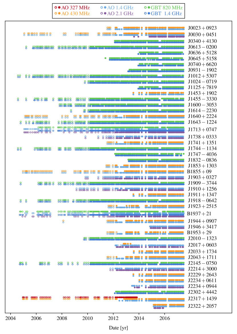
Figure 1: Epochs of all observations in the data set. The observatory and observing frequency are indicated by color: Arecibo observations are red (327 MHz), orange (430 MHz), light blue (1.4 GHz), and purple (2.1 GHz). GBT observations are green (820 MHz) and dark blue (1.4 GHz). The data acquisition system is indicated by symbol: open circles are ASP or GASP, and filled circles are PUPPI or GUPPI.

Two generations of backend instrumentation were used for data collection. The ASP and GASP systems (64 MHz of bandwidth; Demorest, 2007) at Arecibo and the GBT, respectively, were used for approximately the first six years of NANOGrav data acquisition. We transitioned to PUPPI (at Arecibo) and GUPPI (at Green Bank) in 2012 and 2010, respectively. PUPPI and GUPPI have been used for all subsequent data collection, including all new data in the present paper. They can process up to 800-MHz bandwidths (DuPlain et al., 2008; Ford et al., 2010) and significantly improved our timing precision relative to ASP and GASP. During the transition from ASP/GASP to PUPPI/GUPPI, we made precise measurements of time offsets between the instruments (Appendix A of NG9). We continue to use the offset measurements from NG9.

These instruments divide the telescope passband into narrow spectral channels, undertake coherent dedispersion of the signals within each channel, evaluate self- and cross-products to enable recovery of four Stokes parameters, and fold the resulting time series in real time using a nominal pulsar timing model. Thus, the raw data are in the form of folded pulse profiles as a function of time, radio frequency, and polarization. The raw profiles have 2048 phase bins, a frequency resolution of 4 MHz (ASP/GASP) or 1.5 MHz (GUPPI/PUPPI), and subintegrations of 1 second (PUPPI at 1.4 and 2.1 GHz) or 10 seconds (all other receiver/backend combinations).

Observations were calibrated in two steps. Prior to each pulsar observation, we inject a pulsed noise signal into the receiver path for use in calibrating the signal amplitudes. The pulsed noise signals, in turn, are calibrated approximately monthly via a series of on- and off-source observations on an unpolarized continuum radio source of known flux density. Details of the continuum source are given in Section 8.

2.2 ASP/GASP Times-of-Arrival

We collected data using the ASP and GASP instruments through 2012 and 2010, respectively. There are no new ASP/GASP data in this data release. For these data, we used TOAs generated in NG9 without modification. These TOAs were computed using procedures similar to those for PUPPI/GUPPI data described below. The ASP/GASP TOAs incorporate time offsets relative to the PUPPI/GUPPI instruments as described in NG9.

During the transition between the ASP/GASP and PUPPI/GUPPI instruments, parallel data were collected on two instruments, resulting in two (redundant) sets of TOAs. In these situations, we use only the PUPPI/GUPPI TOAs, but we retain the commented-out ASP/GASP TOAs in the data set, flagging these TOAs in a method similar to the cut TOAs described in section 2.5.

2.3 PUPPI/GUPPI Data Reduction

In this section, we describe the processing of PUPPI/GUPPI folded pulse profiles described above to remove various artifacts, to calibrate the data amplitudes, and to produce more compact data sets which were then used for TOA generation.

2.3.1 Artifact Removal

GUPPI and PUPPI employ an interleaved analog-to-digital conversion (ADC) scheme to achieve their wide bandwidths. Rather than a single ADC running at the Nyquist sampling rate of $2B$ (for a bandwidth $B$), two converters are running in parallel at rate $B$, offset in time from each other by half a cycle. If the gain of the two converters is not identical, or if there is a timing skew such that the time offset is not exactly $(2B)^{-1}$, an image rejection artifact will appear in the data. This looks like a copy of the input signal, frequency reversed about the center of the sampled band (Fig. 2, left panel). For pulsar data this artifact appears negatively dispersed and therefore can be distinguished from most typical RFI. The amplitude of the image signal depends on the magnitude of the gain mismatch or timing skew. Gain mismatch results in a constant image ratio versus frequency, while the ratio from timing skew increases with frequency within the sampled band. Kurosawa et al. (2001) present a detailed analysis of this effect in interleaved sampler systems, and derive analytic expressions for the ratio of image to true signal as a function of the mismatch parameters.

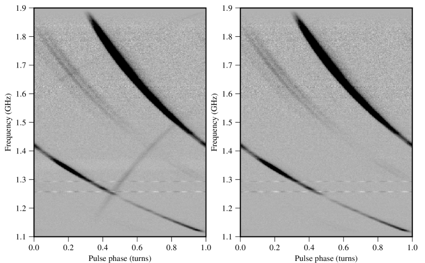
Figure 2: Observation of J1744+1134 illustrating artifacts from GUPPI’s interleaved ADCs. This is one of the lowest-DM pulsars in our sample, therefore the effect is easily visible. Dispersion has not been removed, so the true pulsar signal arrives earlier at higher radio frequencies. The image artifact can be seen as the faint, apparently negatively-dispersed, signal “reflected” about the band center frequency of 1.5 GHz. No interference excision has been applied to these data; the spurious narrowband signals visible between 1.2 and 1.3 GHz are RFI. The plot color scale has been saturated at 10% of the maximum data value. The left panel shows the raw data, while the right panel shows the same data after the correction procedure has been applied.

If not corrected, the presence of these artifacts will result in a frequency-dependent systematic TOA bias. The effect is largest at those points in the band where the image pulse crosses the true pulse. Low-DM, slow-spinning pulsars with wide pulse profile shapes are the most affected, while for high-DM sources dispersion will smear out the image relative to the pulsar signal within each channel, reducing its impact. For J2145$-$0750, a 1% image ratio could shift some individual channel TOAs by up to 1 $\mu$s, while for J1909$-$3744 the effect is 40 ns and confined to smaller parts of the band. On average this effect will cancel out when averaged over the full wide band, with equal amounts of positively and negatively shifted channels, however this depends on the details of bandpass shape and scintillation pattern. In NG11 and previous data sets, there was no effort to mitigate these images. In the present work, we introduce a new procedure to remove the images.

Using data from several bright pulsars in our sample, we measured the relative amplitudes of the pulsar and image signals as a function of frequency, bandwidth, and observing epoch. We find that the observed effect is consistent with a pure timing skew, with a typical value of $\sim$30 ps. This results in image ratios ranging from 0.5% to 4% across the band. The timing skew values are consistent between pulsars for a given backend setup. The values vary with time, showing occasional step-like changes at dates corresponding to known maintenance procedures such as replacement of a faulty ADC board or synthesizer. Based on this observed behavior, we developed a piecewise constant in time model for the skew value that can be used to correct the data.

With the known skew values, we calculate image ratio as a function of frequency following Kurosawa et al. (2001). For all input data, we apply this ratio to a frequency-reversed copy of the data, and subtract the result, giving a corrected data set (Fig. 2, right-hand panel). Based on the scatter of the measured skew values we conservatively estimate this correction is good to at least the 10% level, therefore reducing image artifacts by one order of magnitude.

This procedure relies on having data measured continuously across the full sampled bandwidth, as normally was the case in our observations. However, in the PUPPI data set occasional instrumental failures resulted in portions of the band not being recorded. In these cases, it is not possible to apply the correction to the corresponding subband “mirrored” about the band center. Nevertheless, we elected to include such data in the data set. In the TOA-flagging system described below, TOAs generated from such data are marked using the -img uncorr flag.

2.3.2 Calibration and Integration in Time and Frequency

After removing artifact images, we performed standard data reduction procedures as described in NG11, with one additional step of excising radio frequency interference (RFI) from the calibration files as well as from the data files; this additional step led to improvements in TOA measurements, especially at 2.1 GHz with PUPPI. The remaining steps of calibrating, reducing, and excising RFI from the data were the same as in NG11. Data were frequency-averaged into channels with bandwidths between 1.5 and 12.5 MHz, depending on the receiver. We time-averaged the calibrated and cleaned profiles into subintegrations up to 30 minutes in length, except in the few cases of binary pulsars with very short orbital periods; in those cases we averaged the data into subintegrations no longer in duration than 2.5% of the orbital period in order to maintain time resolution over the orbit.

2.4 PUPPI/GUPPI Time-of-Arrival Generation

We generally followed the methods described in NG9 and NG11 to calculate narrowband TOAs, but with an improved algorithm to calculate TOA uncertainties. The uncertainties were calculated by numerical integration of the TOA probability distribution presented in Eqn. 12 of NG9 Appendix B. This mitigates underestimation of uncertainties calculated by conventional methods in the low-signal-to-noise regime.

We used previously-generated template pulse profiles for the 45 pulsars from NG11, generating new templates only for the two pulsars newly added to this data set. To make the template profiles, we iteratively aligned and averaged together the reduced data profiles, and applied wavelet smoothing to the final average profile. With these templates, we measured TOAs from the reduced GUPPI and PUPPI profiles, and collated them with the existing GASP and ASP TOAs from NG9.

Table 1: TOA Removal Methods

Flag	No. of TOAs	Reason for TOA Removal	Notes (including differences with the
	Removed		wideband data set procedures)
-cut snr	92,290	(Section 2.5.1) Profile data used to generate TOA does not meet signal-to-noise ratio threshold	S/N $<$ 8 for narrowband TOAs, S/N $<$ 25 for wideband TOAs
-cut badepoch	11,650	(Sections 2.5.4, 2.5.5, 2.5.6) Observation is significantly corrupted by instrumentation issues or RFI	Identified by human inspection; these observations are not included in the wideband data set
-cut dmx	10,874	(Section 2.5.2) Ratio of maximum to minimum frequency in an observing epoch (in a single DMX bin) $\nu_{\rm{max}}/\nu_{\rm{min}}<1.1$	$\nu_{\rm{max}}$ and $\nu_{\rm{min}}$ are TOA reference frequencies in the narrowband data set and are separately calculated for each TOA in the wideband data set
-cut simul	5,194	(Section 2.2) ASP/GASP TOA acquired at the same time as a PUPPI/GUPPI TOA	Removed at the last stage of analysis from both narrowband and wideband data sets
-cut epochdrop	2,384	(Section 2.5.7) Entire epoch removed based on $F$-test $p<10^{-6}$	Epochs identified in the narrowband data set analysis are also removed from the wideband data set
-cut outlier10	1,022	(Section 2.5.3) TOA has outlier probability $p_{i,{\rm out}}>0.1$	This particular outlier analysis applies only to the narrowband data set
-cut orphaned	490	(Section 2.5.9) Insignificant data volume	A small number of TOAs originate from test observations in different receiver bands; these observations are not included in the wideband data set
-cut manual	70	(Section 2.5.8) The TOAs corresponding to individual pulse profile are corrupted by instrumentation or RFI, but were not identified and removed via S/N threshold or outlier probability cuts	Identified by human inspection; both narrowband and wideband data sets have a small volume of manually excised TOAs, but they were determined independently

Note. — The flags are listed here in order of the number of narrowband TOAs that were removed from the data set via each method. All cut TOAs are provided as commented-out TOAs in the ASCII-text TOA files; excluding these, there are 415,173 narrowband TOAs in the data set.

2.5 Cleaning the Data Set for Improved Data Quality

Calculated TOAs can be biased by a variety of observational problems, including imperfections in instrumentation, flawed calibration, RFI, or other non-astrophysical influences. In past data releases, we have ensured a high level of data quality by systematically removing RFI, excluding low signal-to-noise (S/N) TOAs (see details in NG9), removing outliers identified by Bayesian analysis of residuals (see details in NG11), and manual inspection of the data sets. These same procedures were carried out for the present data set, along with a series of new cleaning techniques described below.

The remainder of this section details these quality-control measures, which led to the removal of uninformative or suspect TOAs, as well as entire observations in some cases. The data quality analysis steps were typically iterative in nature. For example, the “bad DMX range” criterion described below was re-checked after any change in the data set made for other reasons.

All TOAs removed by these procedures are included in the data set files. They are marked as comments in the TOA files, and each excluded TOA includes a flag indicating the reason for its exclusion. The exclusion methods, flags, and statistics of removed TOAs are summarized in Table 1. After all TOA cutting was complete, the final narrowband data set had 415,173 TOAs.

2.5.1 Signal-to-noise ratio cut

As in NG9 and NG11, we removed TOAs that were generated from pulse profiles with S/N $<$ 8. These TOAs contain little information and, at the very lowest S/N values, can be miscalculated due to the dominance of noise over any pulsar signal that is present. We maintained this S/N cutoff in the present work.

2.5.2 Bad DM range cut

As detailed in Section 3.2, our timing models include a step-wise model for variation in DM, in which DM is allowed to have independently varying values in time intervals. The time intervals range in length from 0.5 to 15 days, depending on the telescope and instrumentation. In order to achieve DM measurements of reasonable precision, we require that the maximum-to-minimum frequency ratio of TOAs with each of these time ranges satisfies $\nu_{\mathrm{max}}/\nu_{\mathrm{min}}>1.1$. Data within any DM time range that did not meet this criterion were removed.

As with NG11, this criterion lead to the removal of some data that had been incorporated in NG9, in particular lengthy subsets of single-receiver data from a few pulsars initially observed as part of a non-NANOGrav timing program and later merged into our data set.

2.5.3 Outlier TOA Cut

We used the automated outlier-identification algorithm of Vallisneri & van Haasteren (2017) to estimate the probability $p_{i,{\rm out}}$ that each individual TOA is an outlier, based on the initial 12.5-year timing models. The $p_{i,{\rm out}}$ are defined in Equation 6 of Vallisneri & van Haasteren, where Equations 1–5 provide definitions of the parameters in Equation 6. The $p_{i,{\rm out}}$ estimate is fully consistent with the Bayesian inference of all noise parameters of the pulsar being analyzed. As in NG11, we removed all TOAs with $p_{i,{\rm out}}>0.1$, resulting in a total of 1,022 TOAs being removed from the full 12.5-year data set. This outlier probability threshold was chosen based on inspection of a subset of pulsars, from which we found that $p_{i,{\rm out}}$ has an extremely bimodal distribution: nearly all TOAs had $p_{i,{\rm out}}<0.1$ or $p_{i,{\rm out}}>0.9$. The $p_{i,{\rm out}}>0.1$ threshold for TOA removal is thus empirically motivated, and additionally remains consistent with the threshold used in NG11.

We note that the outlier analysis was not run iteratively as timing models were updated. Such an iterative procedure was tested on several pulsars, and it was found that the updated outlier results had very minor, if any, differences from the original outlier results. This finding is likely explained by the fact that the results of the outlier runs are already marginalized over the linearized timing model parameters, with very large priors. Thus a different set of outliers from a subsequent analysis would only be expected if the original outliers had taken the timing model outside its linear range, or if so many data points were excluded after the initial analysis that the noise profile changed and new, previously-obscured outliers were revealed. Based on our empirical findings from the iterative outlier analysis runs on a subset of pulsars, and on this theoretical explanation, we chose to only run the outlier analysis once at the beginning of the timing analysis for the full data set.

2.5.4 Manual Removal of Individual Observations Guided by Outlier TOAs

The outlier analysis was used as a guide in identifying observing epochs in which most or all TOAs may have been corrupted by instrumentation issues or by excessive RFI. If a single observation had more than five TOAs with $p_{i,{\rm out}}>0.1$, we reviewed the corresponding observing log and examined the data manually to determine if there were instrumental problems or RFI that rendered the observation unusable. In such cases, all TOAs from the affected observations were removed.

2.5.5 Corrupt Calibration Cut

As described above, pulsar observations were preceded by measurements using an artificial pulsed noise signal injected in the telescope signal path, and the same pulsed-noise-signal method was used during continuum calibrator observations. We searched for anomalies in the pulsed-noise-signal measurements; these could result from instrumentation failures or from use of incorrect noise signals in an individual observation.

The following are specific anomalies that were identified in the calibration files. (1) A pulsed-noise amplitude that was unusually high or low (88 affected observations). (2) Cross-polarization flux calibration amplitudes deviating significantly from the mean locus of amplitudes for a given receiver/backend combination (65 observations affected and removed, due to corrupted continuum source observations on MJDs 57229 and 57249). (3) Pulsed calibrator phase not smoothly varying with frequency (one observation was removed solely for this reason, but this was also seen in observations flagged for othe reasons). (4) Polarization fraction, $f_{UV}=[(U^{2}+V^{2})/I^{2}]^{1/2}$, deviating from expected values. For pulsars with high intrinsic polarization ($f_{UV}\sim 1$), a small number of observations had significantly lower estimated $\hat{f}_{UV}$ values (typically $\hat{f}_{UV}<0.3$) that signified corrupted data, and a small number of profiles had $\hat{f}_{UV}>1$, suggesting a problem with the digitization levels (23 affected observations).

2.5.6 Flux Measurement Cut

Extremely high or low apparent flux density values can result from incorrect calibration or digitization levels. We therefore searched for outlier flux densities as a proxy for calibration errors not detected through the means listed above. We manually examined such observations and removed them as needed. Only one observation was identified and removed by this method, but this analysis informed the development of our other quality-check methods. A detailed flux density analysis is in Section 8.

2.5.7 Epoch $F$-Test Cut

We tested for the presence of otherwise-undetected bad data for each pulsar by removing data from one observing epoch at a time and examining its impact on the timing residuals. This method is effectively an outlier analysis for full observing epochs, rather than for individual TOAs. We compared the chi-square of the timing residuals before and after data removal, $\chi^{2}_{0}$ and $\chi^{2}$, respectively, using an $F$-statistic,

$$F=\frac{(\chi^{2}_{0}-\chi^{2})/(n_{0}-n)}{(\chi^{2}/n)},$$ (1)

where $n_{0}$ and $n$ are the number of degrees of freedom in the original and epoch-removed analyses. We removed data for epochs for which the $F$-test reported a chance probability $p<10^{-6}$ ($\sim$ 5$\sigma$). This process was run iteratively. We examined the profiles and calibration files for a subset of the observations that were flagged in this way and found that a majority of these observations were faulty in obvious ways (calibration errors, extreme RFI, etc.).

2.5.8 Manual TOA Cut

After completing the above data quality checks, uninformative or outlying TOAs were still present in the data sets of some pulsars. A total of 70 additional TOAs were removed after visual inspection. These were TOAs whose timing residuals appeared to be outliers but were not flagged by the outlier analysis (typically a small number of pulse profiles had been corrupted by narrow-frequency RFI, such that TOAs in a subset of the full bandwidth had to be removed but the rest of the profile or epoch was not adversely affected) or TOAs with very large uncertainties and large timing residuals (usually resulting from a low-S/N TOA measurement, just above our cutoff threshold, or RFI).

2.5.9 Orphan Data Cut

For a few pulsars, in addition to the receivers normally used for observations, a small number of observations were made with a different receiver, typically for testing purposes near the start of observations of this source. We cut such TOAs in the same manner as data that were cut for other reasons.

2.5.10 Wideband TOA Residual Check

We note that for the methods described above, in some cases it was difficult to determine if data were corrupted (e.g., the residuals from a given epoch may have been larger than expected, but no evidence of an issue with the calibration or profile data was found upon inspection). In those cases, we also examined the residual profiles generated from fitting wideband TOAs, which use high-fidelity, evolving profile models in the matched-template algorithm. For example, the residual profile may reveal that the evolving profile model did not adequately represent the profile during that observation, suggesting a problem with the data that was not found using other methods. Inspection of the wideband residual profiles thus aided in identifying and removing more corrupted data in the narrowband data set. Using the evolving profile models as a means to identify corrupted data profiles is an ongoing development.

3 Timing Analysis

Table 2: Basic Pulsar Parameters and TOA Statistics

Source	$P$	$dP/dt$	DM	$P_{b}$	Median scaled TOA uncertaintya ($\mu$s) / Number of epochs										Span
	(ms)	($10^{-20}$)	(pc cm-3)	(d)	327 MHz		430 MHz		820 MHz		1.4 GHz		2.1 GHz		(yr)
J0023$+$0923	3.05	1.14	14.3	0.1	$\cdots$		0.063	62	$\cdots$		0.556	68	$\cdots$		6.0
J0030$+$0451	4.87	1.02	4.3	-	$\cdots$		0.214	175	$\cdots$		0.424	187	1.558	71	12.4
J0340$+$4130	3.30	0.70	49.6	-	$\cdots$		$\cdots$		0.868	68	2.108	71	$\cdots$		5.3
J0613$-$0200	3.06	0.96	38.8	1.2	$\cdots$		$\cdots$		0.109	134	0.582	135	$\cdots$		12.2
J0636$+$5128	2.87	0.34	11.1	0.1	$\cdots$		$\cdots$		0.279	39	0.579	42	$\cdots$		3.5
J0645$+$5158	8.85	0.49	18.2	-	$\cdots$		$\cdots$		0.297	67	0.836	74	$\cdots$		6.1
J0740$+$6620	2.89	1.22	15.0	4.8	$\cdots$		$\cdots$		0.445	38	0.651	40	$\cdots$		3.5
J0931$-$1902	4.64	0.36	41.5	-	$\cdots$		$\cdots$		1.030	51	1.777	53	$\cdots$		4.3
J1012$+$5307	5.26	1.71	9.0	0.6	$\cdots$		$\cdots$		0.403	135	0.725	143	$\cdots$		12.9
J1024$-$0719	5.16	1.86	6.5	-	$\cdots$		$\cdots$		0.520	90	0.981	94	$\cdots$		7.7
J1125$+$7819	4.20	0.69	12.0	15.4	$\cdots$		$\cdots$		0.974	40	2.024	42	$\cdots$		3.5
J1453$+$1902	5.79	1.17	14.1	-	$\cdots$		1.141	35	$\cdots$		2.120	40	$\cdots$		3.9
J1455$-$3330	7.99	2.43	13.6	76.2	$\cdots$		$\cdots$		1.100	115	1.937	117	$\cdots$		12.9
J1600$-$3053	3.60	0.95	52.3	14.3	$\cdots$		$\cdots$		0.271	113	0.227	115	$\cdots$		9.6
J1614$-$2230	3.15	0.96	34.5	8.7	$\cdots$		$\cdots$		0.374	96	0.593	107	$\cdots$		8.8
J1640$+$2224	3.16	0.28	18.5	175.5	$\cdots$		0.048	180	$\cdots$		0.375	189	$\cdots$		12.3
J1643$-$1224	4.62	1.85	62.3	147.0	$\cdots$		$\cdots$		0.288	131	0.499	131	$\cdots$		12.7
J1713$+$0747	4.57	0.85	15.9	67.8	$\cdots$		$\cdots$		0.188	129	0.077	451	0.061	186	12.4
J1738$+$0333	5.85	2.41	33.8	0.4	$\cdots$		$\cdots$		$\cdots$		0.520	71	0.901	68	7.6
J1741$+$1351	3.75	3.02	24.2	16.3	$\cdots$		0.142	63	$\cdots$		0.352	73	$\cdots$		5.9
J1744$-$1134	4.07	0.89	3.1	-	$\cdots$		$\cdots$		0.155	130	0.237	128	$\cdots$		12.9
J1747$-$4036	1.65	1.31	153.0	-	$\cdots$		$\cdots$		1.033	61	1.160	65	$\cdots$		5.3
J1832$-$0836	2.72	0.83	28.2	-	$\cdots$		$\cdots$		0.596	53	0.524	53	$\cdots$		4.3
J1853$+$1303	4.09	0.87	30.6	115.7	$\cdots$		0.353	67	$\cdots$		0.593	72	$\cdots$		6.0
B1855$+$09….	5.36	1.78	13.3	12.3	$\cdots$		0.208	117	$\cdots$		0.211	124	$\cdots$		12.5
J1903$+$0327	2.15	1.88	297.5	95.2	$\cdots$		$\cdots$		$\cdots$		0.443	75	0.511	78	7.6
J1909$-$3744	2.95	1.40	10.4	1.5	$\cdots$		$\cdots$		0.066	126	0.124	269	$\cdots$		12.7
J1910$+$1256	4.98	0.97	38.1	58.5	$\cdots$		$\cdots$		$\cdots$		0.338	82	0.767	83	8.3
J1911$+$1347	4.63	1.69	31.0	-	$\cdots$		0.590	42	$\cdots$		0.157	46	$\cdots$		3.9
J1918$-$0642	7.65	2.57	26.5	10.9	$\cdots$		$\cdots$		0.518	126	0.901	128	$\cdots$		12.7
J1923$+$2515	3.79	0.96	18.9	-	$\cdots$		0.259	55	$\cdots$		1.023	67	$\cdots$		5.8
B1937$+$21….	1.56	10.51	71.1	-	$\cdots$		$\cdots$		0.007	127	0.014	220	0.018	86	12.8
J1944$+$0907	5.19	1.73	24.4	-	$\cdots$		0.278	63	$\cdots$		0.825	73	$\cdots$		9.3
J1946$+$3417	3.17	0.32	110.2	27.0	$\cdots$		$\cdots$		$\cdots$		0.414	40	0.547	39	2.6
B1953$+$29….	6.13	2.97	104.5	117.3	$\cdots$		0.255	54	$\cdots$		0.815	65	$\cdots$		5.9
J2010$-$1323	5.22	0.48	22.2	-	$\cdots$		$\cdots$		0.412	94	0.983	96	$\cdots$		7.8
J2017$+$0603	2.90	0.80	23.9	2.2	$\cdots$		0.195	6	$\cdots$		0.425	67	0.537	50	5.3
J2033$+$1734	5.95	1.11	25.1	56.3	$\cdots$		0.194	40	$\cdots$		1.163	46	$\cdots$		3.8
J2043$+$1711	2.38	0.52	20.8	1.5	$\cdots$		0.079	137	$\cdots$		0.281	151	$\cdots$		5.9
J2145$-$0750	16.05	2.98	9.0	6.8	$\cdots$		$\cdots$		0.289	111	0.650	116	$\cdots$		12.8
J2214$+$3000	3.12	1.47	22.5	0.4	$\cdots$		$\cdots$		$\cdots$		0.743	72	1.059	57	5.7
J2229$+$2643	2.98	0.15	22.7	93.0	$\cdots$		0.324	45	$\cdots$		1.096	47	$\cdots$		3.9
J2234$+$0611	3.58	1.20	10.8	32.0	$\cdots$		0.429	41	$\cdots$		0.221	45	$\cdots$		3.4
J2234$+$0944	3.63	2.01	17.8	0.4	$\cdots$		$\cdots$		$\cdots$		0.314	45	0.746	44	4.0
J2302$+$4442	5.19	1.39	13.8	125.9	$\cdots$		$\cdots$		1.200	69	2.413	68	$\cdots$		5.3
J2317$+$1439	3.45	0.24	21.9	2.5	0.085	79	0.068	188	$\cdots$		0.642	141	$\cdots$		12.5
J2322$+$2057	4.81	0.97	13.4	-	$\cdots$		0.291	35	$\cdots$		1.021	34	1.431	10	2.3
Nominal scaling factorb (ASP/GASP)					0.6		0.4		0.8		0.8		0.8
Nominal scaling factorb (GUPPI/PUPPI)					0.7		0.5		1.4		2.5		2.1

^a For this table, the original TOA uncertainties were scaled by their bandwidth-time product $\left(\frac{\Delta\nu}{100~{}\mathrm{MHz}}\frac{\tau}{1800~{}\mathrm{s}}\right)^{1/2}$ to remove variation due to different instrument bandwidths and integration time. We note that in NG11, we incorrectly calculated the tabulated TOA uncertainties due to a scripting error. This generally led to overestimates of the uncertainty at lower frequencies and underestimates at higher frequencies. The error only applied to values shown in Table 1 of NG11, and did not affect the released data or any other results in the paper. We have corrected this error for the present work.

^b TOA uncertainties can be rescaled to the nominal full instrumental bandwidth as listed in Table 1 of Arzoumanian et al. (2015) by dividing by the scaling factors given here.

Table 3: Summary of Timing Model Fits

Source	Number	Number of Fit Parametersa						RMSb ($\mu$s)		Red Noisec			Figure
	of TOAs	S	A	B	DM	FD	J	Full	White	$A_{\mathrm{red}}$	$\gamma_{\mathrm{red}}$	log${}_{10}B$	Number
J0023$+$0923	12516	3	5	9	67	4	1	0.285	$\cdots$	$\cdots$	$\cdots$	1.21	6
J0030$+$0451	12543	3	5	0	190	4	2	25.157	0.200	0.003	$-$6.3	$>$2	7
J0340$+$4130	8069	3	5	0	74	4	1	0.446	$\cdots$	$\cdots$	$\cdots$	$-$0.21	8
J0613$-$0200	13201	3	5	8	139	2	1	0.486	0.178	0.123	$-$2.1	$>$2	9
J0636$+$5128	21374	3	5	6	44	1	1	0.640	$\cdots$	$\cdots$	$\cdots$	$-$0.09	10
J0645$+$5158	7893	3	5	0	79	2	1	0.207	$\cdots$	$\cdots$	$\cdots$	$-$0.20	11
J0740$+$6620	3328	3	5	7	44	1	1	0.132	$\cdots$	$\cdots$	$\cdots$	$-$0.17	12
J0931$-$1902	3712	3	5	0	57	0	1	0.452	$\cdots$	$\cdots$	$\cdots$	$-$0.15	13
J1012$+$5307	19307	3	5	6	142	4	1	0.999	0.272	0.406	$-$1.6	$>$2	14
J1024$-$0719	9792	4	5	0	100	2	1	0.334	$\cdots$	$\cdots$	$\cdots$	$-$0.08	15
J1125$+$7819	4821	3	5	5	43	3	1	0.862	$\cdots$	$\cdots$	$\cdots$	0.09	16
J1453$+$1902	1555	3	5	0	39	0	1	0.606	$\cdots$	$\cdots$	$\cdots$	$-$0.13	17
J1455$-$3330	8408	3	5	6	122	2	1	0.656	$\cdots$	$\cdots$	$\cdots$	$-$0.14	18
J1600$-$3053	14374	3	5	8	128	2	1	0.245	$\cdots$	$\cdots$	$\cdots$	0.55	19
J1614$-$2230	12775	3	5	8	114	2	1	0.177	$\cdots$	$\cdots$	$\cdots$	$-$0.24	20
J1640$+$2224	9256	3	5	8	188	4	1	0.177	$\cdots$	$\cdots$	$\cdots$	$-$0.20	21
J1643$-$1224	12798	3	5	6	141	2	1	2.645	0.534	1.498	$-$1.4	$>$2	22
J1713$+$0747	37698	3	5	8	325	5	3	0.101	0.069	0.030	$-$1.3	$>$2	23
J1738$+$0333	6977	3	5	5	78	1	1	0.276	$\cdots$	$\cdots$	$\cdots$	$-$0.24	24
J1741$+$1351	3845	3	5	8	73	2	1	0.156	$\cdots$	$\cdots$	$\cdots$	$-$0.08	25
J1744$-$1134	13380	3	5	0	136	4	1	0.832	0.307	0.155	$-$2.2	$>$2	26
J1747$-$4036	7572	3	5	0	71	1	1	6.343	1.414	0.709	$-$3.3	$>$2	27
J1832$-$0836	5364	3	5	0	58	0	1	0.187	$\cdots$	$\cdots$	$\cdots$	$-$0.05	28
J1853$+$1303	3544	3	5	8	72	0	1	0.392	0.110	0.140	$-$2.2	$>$2	29
B1855$+$09….	6464	3	5	7	125	3	1	1.757	0.357	0.054	$-$3.4	$>$2	30
J1903$+$0327	4854	3	5	8	82	1	1	2.668	0.315	1.482	$-$1.6	$>$2	31
J1909$-$3744	22633	3	5	9	223	1	1	0.334	0.061	0.028	$-$2.7	$>$2	32
J1910$+$1256	5012	3	5	6	88	1	1	0.187	$\cdots$	$\cdots$	$\cdots$	$-$0.06	33
J1911$+$1347	2625	3	5	0	46	2	1	0.118	$\cdots$	$\cdots$	$\cdots$	0.20	34
J1918$-$0642	13675	3	5	7	133	5	1	0.299	$\cdots$	$\cdots$	$\cdots$	0.02	35
J1923$+$2515	3009	3	5	0	67	1	1	0.269	$\cdots$	$\cdots$	$\cdots$	$-$0.15	36
B1937$+$21….	17024	3	5	0	204	5	3	2.277	0.103	0.099	$-$3.3	$>$2	37
J1944$+$0907	3931	3	5	0	73	2	1	0.365	$\cdots$	$\cdots$	$\cdots$	0.12	38
J1946$+$3417	3016	3	5	8	41	1	1	0.468	$\cdots$	$\cdots$	$\cdots$	1.77	39
B1953$+$29….	3421	3	5	6	65	2	1	0.475	$\cdots$	$\cdots$	$\cdots$	1.05	40
J2010$-$1323	13306	3	5	0	108	1	1	0.244	$\cdots$	$\cdots$	$\cdots$	$-$0.22	41
J2017$+$0603	2986	3	5	7	73	0	2	0.076	$\cdots$	$\cdots$	$\cdots$	$-$0.22	42
J2033$+$1734	2691	3	5	5	46	2	1	0.561	$\cdots$	$\cdots$	$\cdots$	$-$0.12	43
J2043$+$1711	5624	3	5	7	151	4	1	0.151	$\cdots$	$\cdots$	$\cdots$	1.41	44
J2145$-$0750	13961	3	5	7	123	2	1	1.467	0.328	0.347	$-$2.1	$>$2	45
J2214$+$3000	6269	3	5	5	77	1	1	0.402	$\cdots$	$\cdots$	$\cdots$	$-$0.17	46
J2229$+$2643	2442	3	5	6	47	2	1	0.194	$\cdots$	$\cdots$	$\cdots$	$-$0.18	47
J2234$+$0611	2475	3	5	7	45	2	1	0.061	$\cdots$	$\cdots$	$\cdots$	0.60	48
J2234$+$0944	5892	3	5	5	51	2	1	0.160	$\cdots$	$\cdots$	$\cdots$	$-$0.13	49
J2302$+$4442	7833	3	5	7	75	1	1	0.716	$\cdots$	$\cdots$	$\cdots$	$-$0.15	50
J2317$+$1439	9835	3	5	6	210	3	2	8.798	0.253	0.007	$-$6.4	$>$2	51
J2322$+$2057	2093	3	5	0	35	4	2	0.235	$\cdots$	$\cdots$	$\cdots$	$-$0.13	52

^a Fit parameters: S=spin; A=astrometry; B=binary; DM=dispersion measure; FD=frequency dependence; J=jump

^b Weighted root-mean-square of epoch-averaged post-fit timing residuals, calculated using the procedure described in Appendix D of NG9. For sources with red noise, the “Full” RMS value includes the red noise contribution, while the “White” RMS does not.

^c Red noise parameters: $A_{\mathrm{red}}$ = amplitude of red noise spectrum at $f$=1 yr^-1 measured in $\mu$s yr^1/2; $\gamma_{\mathrm{red}}$ = spectral index; $B$ = Bayes factor (“$>$2” indicates a Bayes factor larger than our threshold log₁₀B $>$ 2, but which could not be estimated using the Savage-Dickey ratio). See Eqn. 2 and Appendix C of NG9 for details.

The cleaned TOA data set for each pulsar was fit with a physical timing model, with the Tempo timing software used for the primary analysis. The timing models were checked using the Tempo2 and PINT packages. PINT (Luo et al., 2019, 2020) was developed independently of Tempo and Tempo2 and thus provides a particularly robust independent check of the timing models (Section 4). Our expectation is to transition to PINT as the primary timing software for future data sets due to its modularity and its use of modern programming tools, including coding in Python.

An overarching development in the current release is our use of standardized and automated timing procedures. In previous NANOGrav data releases, two core portions of the data analysis were already automated: data reduction (calibration, RFI removal, time- and frequency-averaging) and TOA generation, all of which was done using nanopipe (Demorest, 2018); and checking for timing parameter significance (e.g., as in NG11). For the 12.5-year data set, we standardized and automated the timing procedure using Jupyter notebooks. These notebooks did not replace the often iterative nature of pulsar timing. Rather, once a reasonable timing solution was found for a pulsar, it was input into the notebook, which ran through an entire standard analysis that included checking for parameter significance (Section 3.1) and performing noise modeling (Section 3.3). This process allowed for systematic and transparent addition or removal of timing and noise parameters, and ensured that the final timing models were assembled in a standardized way. Additional benefits of automating the timing analysis in this way are that it makes NANOGrav timing analysis more accessible to new students or researchers, and much of the automated process can also be applied to other (non-PTA) pulsar timing work.

3.1 Timing Models and Parameters

Timing fits were done using the JPL DE436 solar system ephemeris and the TT(BIPM2017) timescale. As in previous releases, we used a standard procedure to determine which parameters are included in each pulsar’s timing model. Always included as free parameters were the intrinsic spin and spin-down rate, and five astrometric parameters (two position parameters, two proper motion parameters, and parallax), regardless of measurement significance. We used ecliptic coordinates for all astrometric parameters to minimize parameter covariances. For binary pulsars, five Keplerian parameters were also always fit: (i) the orbital period, ($P_{b}$) or orbital frequency ($F_{b}$); (ii) the projected semi-major axis ($x$); and (iii-v) either the eccentricity ($e$), longitude of periastron ($\omega$), and epoch of periastron passage ($T_{0}$); or two Laplace-Lagrange parameters ($\epsilon_{1}$, $\epsilon_{2}$) and the epoch of the ascending node ($T_{\mathrm{asc}}$).

The particular binary model chosen was based on orbital characteristics, including the presence of post-Keplerian parameters. For low-eccentricity orbits, we used the ELL1 model, which approximates the orbit using the Laplace-Lagrange parameterization of the eccentricity with $\epsilon_{1}$ and $\epsilon_{2}$ (Lange et al., 2001). In all cases in which we used ELL1, the model deviated from a more precise timing model by at most 25 ns at any point in the orbit. The pulsars in this data set that satisfy this criterion for the use of the ELL1 model all have $e<10^{-5}$, although we did not apply an explicit eccentricity criterion for this binary model. If Shapiro delay was marginally present in a low-eccentricity system, we used ELL1H, which incorporates the orthometric parameterization of the Shapiro delay (Freire & Wex, 2010) into the ELL1 model; note that the ELL1H model employs the $h_{3}$ and $h_{4}$ parameters, as opposed to $h_{3}$ and $\varsigma=h_{4}/h_{3}$ of the DDFWHE model (Freire & Wex, 2010; Weisberg & Huang, 2016), which is for high-eccentricity systems and is not used in any timing models in this data set. For pulsars with higher eccentricity, we used the DD binary model (Damour & Deruelle, 1985, 1986; Damour & Taylor, 1992); and for PSR J1713+0747, we used DDK (Kopeikin, 1995, 1996), which allows us to measure annual-orbital parallax. For PSR J1713+0747, a Tempo2-compatible timing model that uses the T2 binary model instead of DDK is also included in the data release. For some short-period binaries ($P_{b}\lesssim 0.5$ d), we used orbital frequency and one or more orbital frequency derivatives, rather than period and period derivative, to better describe the orbit and allow for simple testing of additional orbital frequency derivatives.

We determined parameter significance via an $F$-test, with the requirement that $p<0.0027$ ($\sim$ 3$\sigma$) for a parameter to be included in the timing model. This requirement does not apply to the five astrometric and five Keplerian binary parameters that are always included in the fit (for very low-eccentricity binaries, the eccentricity parameters $\epsilon_{1}$ and $\epsilon_{2}$ may not be measured at a significant level for many years). We specifically tested for the significance of additional frequency-dependent pulse shape or evolution parameters (“FD” parameters; see NG9). We allowed FD1 through FD5 to be fit, and require that all FD parameters up to the highest-order significant FD parameter be included in the fit, even if the lower-order parameters are not found to be significant. For example, if FD4 is significant but FD3 is not, then FD3 would still be included in the timing model.

For binary pulsars, we tested for the secular evolution of binary parameters (e.g., $\dot{x}$, $\dot{\omega}$, or $\dot{P_{b}}$), higher-order orbital frequency derivatives if using orbital frequency rather than period, and Shapiro delay parameters. For binaries modeled by ELL1 without previously-measured Shapiro delay parameters, we converted the binary model to ELL1H and tested the significance of $h_{3}$ and $h_{4}$. If both $h_{3}$ and $h_{4}$ were significant, it raised the possibility of measuring the traditional Shapiro delay parameters (orbital inclination $i$ and companion mass $m_{\mathrm{c}}$) directly from the timing model fit. Thus, for pulsars with significant detections of $h_{3}$ and $h_{4}$, we also tested the use of the traditional Shapiro delay parameters with the ELL1 model: if $i$ and $m_{\mathrm{c}}$ converged to physically meaningful and significantly-measured values, and if the use of these parameters significantly improved the fit according to a $\Delta\chi^{2}$ test, then we included $i$ and $m_{\mathrm{c}}$ in the timing model; otherwise, we continued to use $h_{3}$ and $h_{4}$. Compared with NG11, these significance tests resulted in the inclusion of one or more new binary parameters for 19 pulsars, and the exclusion of previously-included parameters for 3 pulsars (Section 5).

Constant phase “jumps” were included as fit parameters to account for unknown offsets between data subsets collected with different receivers and/or telescopes. For data subsets collected with the same receiver and telescope but different back end instruments, the measured offsets between GASP and GUPPI, and ASP and PUPPI, from NG9 are included in the TOA data set (with flag “-to” on the TOA lines) rather than in the timing model.

We included white and red noise models as described in Section 3.3. We derived best-fit timing model parameter values using a generalized-least-squares fit that uses the noise-model covariance. It is important that the noise model be included when testing for parameter significance, especially if a pulsar shows significant red noise; for several pulsars, one or more parameters were found to be significant when Tempo was run without generalized-least-squares fitting, but were no longer significant when the noise model was included. Thus, the $F$-test significance tests described above were always performed with generalized-least-squares fitting.

A summary of TOA statistics, basic timing parameters, noise parameters, and other statistics are provided in Tables 2 and 3.

3.2 Dispersion Measure Variations

Variations in dispersion measure are caused by the relative motion of the Earth-pulsar sightline through the ionized interstellar medium (IISM) as well as the Earth’s motion through the ionized solar wind, and lead to variations in pulse arrival times. It is therefore necessary to include short-timescale DM variations in the timing model (Jones et al., 2017).

We used the piecewise-constant model called DMX in both Tempo and PINT to measure the short-timescale DM variations in our data set. All Arecibo data were grouped into DMX windows of 0.5 d, because observations of any given pulsar normally use two receivers back-to-back. For the GBT, observations with separate receivers are made on different days; we grouped GASP data into 15 d time ranges, and we grouped GUPPI data into 6.5 d time ranges in order to include data from multiple receivers in most DMX windows. We imposed a minimal frequency range criteria for each DMX window; this is described in section 2.5.2.

If within these DMX time ranges we found that the expected solar wind contribution to the epoch-specific DM induced a timing variation of more than $100$ ns, those time ranges were further divided into 0.5 d windows (thus effectively measuring the DMX for a single observing day). We used a toy model as in NG11 to estimate the expected solar wind-induced time delays: the solar wind electron density is modeled as $n_{e}=n_{0}(r/r_{0})^{-2}$ (where $r$ is the distance from the Sun and $n_{0}$ is the electron density at $r_{0}=1$ AU), and use a representative value of $n_{0}=5$ cm^-3 (e.g., Splaver et al., 2005). (A similar value of 7.9 cm^-3 was found by Madison et al., 2019, with NG11 data.) Additionally, for PSR J1713+0747, it was necessary to break up the DMX time range surrounding its second chromatic event (Lam et al., 2018b): the DM changes so rapidly that using only a single DMX value over the full length of the event introduces significant noise into the data set. The original DMX time range spanned MJD 57508.36–57512.3; we divided this time range into two ranges, spanning MJD 57508.36–57510.36 and 57510.36–57512.3.

3.3 Noise Modeling

The noise model used in this analysis is nearly identical to that of NG9 and NG11. The primary difference is that in this work we used the new PTA analysis software ENTERPRISE (Ellis et al., 2019). In all cases, the final noise model assumes Gaussian noise after all outlier TOAs and otherwise corrupted TOA data have been removed from the data set.

Noise in the timing residuals is modeled as additive Gaussian noise with three white-noise components and, if significantly detected, one red-noise component. For convenience, here we provide a qualitative description of the noise model; for more details, we refer the reader to NG9 and NG11. The four noise components are:

1. EFAC, $E_{k}$: Measured TOA uncertainties $\sigma_{i}$ may be underestimated. A separate EFAC parameter, $E_{k}$, is therefore used for each combination of pulsar, backend, and receiver, indexed by $k$, to account for any systematics in TOA measurement uncertainties; hence $\sigma_{i}$ becomes $\sigma_{i,k}$. For the majority of NANOGrav pulsars, $E_{k}\sim 1$, suggesting that our observing and analysis procedures are resulting in near-true TOA uncertainty estimates.

2. EQUAD, $Q_{k}$: Within ENTERPRISE, the EQUAD term is added in quadrature to the EFAC-scaled TOA uncertainty, i.e., $\sigma^{\prime}_{i,k}=(E_{k}^{2}\sigma_{i,k}^{2}+Q_{k}^{2})^{1/2}$. This term accounts for any uncorrelated systematic white noise that is present in addition to the statistical uncertainties in the TOA calculations. As with EFAC, we use a separate EQUAD parameter, $Q_{k}$, for each combination of pulsar, backend, and receiver, indexed by $k$. Tempo uses a different white noise formulation such that the maximum likelihood EQUAD values contained within the timing models in this data release were obtained via the conversion $Q_{k,\textrm{{\sc Tempo}}}=Q_{k}/E_{k}$.

3. ECORR: This parameter describes a short-timescale noise process that has no correlation between observing epochs, but is completely correlated between TOAs that were obtained simultaneously at different observing frequencies (see Appendix C of NG9 for details). Wideband noise processes such as pulse jitter (Lam et al., 2016; Shannon et al., 2014; Osłowski et al., 2011) are accounted for by ECORR.

4. Red noise: Any steep-spectrum noise components are modeled as a single stationary Gaussian process, whose spectrum we parameterize by a power-law,

   $$P(f)=A^{2}_{\mathrm{red}}\left(\frac{f}{1\,\textrm{yr}^{-1}}\right)^{\gamma_{\mathrm{red}}},$$ (2)

   where $f$ is a given Fourier frequency in the power spectrum and $A_{\mathrm{red}}$ is the amplitude of the red noise at reference frequency 1 yr^-1.

For each pulsar, we incorporated all noise components and timing model parameters into a joint likelihood using ENTERPRISE and sampled the posterior distribution using the sampler PTMCMC (Ellis & van Haasteren, 2017). The red noise prior distribution was log-uniform, while all other prior distributions were uniform. Since the model without red noise is nested within the general model (corresponding to a red noise amplitude of zero), we used the Savage-Dickey ratio to estimate the Bayes factor favoring the presence of red noise (Dickey, 1971). For pulsars with red noise Bayes factor $B$ above a threshold of $B>100$, we included the red noise parameters in the final timing models; for the rest of the pulsars, we re-ran their analyses without red noise. This exercise typically did not affect the detectability of other parameters, but in a small number of cases the presence or absence of red noise did affect marginal timing parameters like $\dot{x}$, $\epsilon_{1}$, or $\epsilon_{2}$ (see the discussion of the PSR J1909$-$3744 binary model in section 7).

The Savage-Dickey ratio fails to estimate a finite Bayes factor for heavily preferred red noise models with a finite-length chain of samples. Indeed, for all of the pulsars with above-threshold red noise, $B$ was large enough that it was not robustly estimated. As such, we simply report the log${}_{10}B$ for those pulsars in Table 2 as $>$2. Further details on the red noise characterization are provided in NG9 and NG11, and Appendix C of NG9 provides a complete description of the Bayesian inference model.

Fourteen pulsars were found to have red noise with $B>100$; this includes all eleven sources with detected red noise in NG11. Of the three MSPs with newly detected red noise (J1744$-$1134, J1853$+$1303, and J2317$+$1439), two of them are among the longest-observed pulsars in the data set.

The Bayes factors for the pulsars in which red noise was not detected are listed in Table 3. Several pulsars have sub-threshold Bayes factors sufficiently larger than 1, such that we may expect those pulsars to display red noise above our defined threshold with several more years of data. A more detailed noise analysis of each pulsar is beyond the scope of this work, but will be performed as part of the gravitational wave analyses for the data set in a forthcoming work.

Table 4: Noise Parameter Comparison for 11-Year Data Subset

Noise Parameter	# Decreaseda	# Increaseda	Mean Differenceb
EFAC	$109$	$30$	$-0.044$
EQUAD	$60$	$79$	$-0.013\;\mu$s
ECORR	$79$	$60$	$-0.017\;\mu$s

^aThe number of noise parameters whose values decreased or increased in the 11-year “slice” of the 12.5-year data set, compared with their values from the 11-year data set (Section 3.4).

^bWeighted mean difference in noise parameters. These are computed as the difference between the 11-year data set values and the 11-year “slice” values, weighted by the errors on the 11-year data set values.

3.4 Improved Noise Parameters over the 11-year Data Set

Our data reduction methods (Section 2.3) and data cleaning methods (Section 2.5) are designed to minimize non-astrophysical noise sources in the data set. Minimizing these noise sources is important because both white noise and red noise have important consequences for the detection of nanohertz gravitational waves (Hazboun et al., 2020; Lam et al., 2018a, 2016; Siemens et al., 2013).

Here we test the methods used in the present work with our previous-generation NG11 data set to see whether the refined methods result in a reduction of noise. To make this comparison with NG11, we use a subset of the present data set that corresponds to the pulsars and date range of NG11, i.e., a data set equivalent to “generating a NG11 data set with procedures of the present work.” A full noise analysis was done on this data subset, consistent with the analyses done in NG11. This sliced analysis has the advantage of using the same timespan of data, which avoids biases from searching for different frequencies of a steep spectral-index red process. Using the same timespan also keeps the number of TOAs in a receiver+backend combination similar so there is no bias in determining white noise parameters with largely differing numbers of TOAs. While a refit to the timing model is out of the scope of such a comparison, the data sets are otherwise similar except for the various data pipeline improvements referenced above. For the pulsars considered for this analysis, there were $139$ pulsar-receiver-backend combinations analyzed, and the changes in their white noise parameters are shown in Table 4. The most dramatic change is seen in the EFAC parameters, where $109$ parameters had EFAC values smaller than in NG11, with a mean difference of $-0.044$. Both the mean EQUAD and ECORR also decrease, but by smaller amounts. The changes in red noise are more subtle, with some pulsars showing mildly increased support for steep spectral index noise processes. These will be discussed in detail in the forthcoming paper presenting our results from GW analyses.

4 Comparison of Tempo and PINT Timing Models

The NANOGrav 12.5-year data analysis results are cross-checked by the new timing package PINT (version 0.5.7), which has a completely independent code base from Tempo and Tempo2. In this section, we present a comparison between the PINT and Tempo timing results for the narrowband TOA data set. This comparison focuses on the discrepancies of the post-fit parameter values. We used timing models produced by Tempo as the initial input models for PINT, and refit the TOAs with PINT’s general least-squares fitter. Then, the best-fit parameters from these two packages were compared against each other. The noise parameters obtained by the ENTERPRISE analysis (Section 3.3) were not altered by PINT, thus we do not compare the noise parameters. To describe the changes of parameter values with an intuitive, standardized quantity, we divide the parameter value differences by the Tempo uncertainties. We have compared 5,417 parameters in total; 3,929 best-fit parameter values from PINT deviate from the Tempo values by less than 5% of their Tempo uncertainties. Among the rest, 1,442 parameters’ PINT results changed by less than 50% of their Tempo uncertainties (for example, changes of the order $10^{-14}$–$10^{-10}$ Hz for spin frequencies, or $10^{-11}$–$10^{-3}$ d for orbital periods), and 46 parameters’ discrepancies are more significant than 50%.

A majority of the outstanding discrepancies ($>$50% of Tempo uncertainty) can be explained by different implementations in the two software packages. Thirty-two of these outlier parameters belong to the two pulsars that have the largest amplitude of red noise, J1643$-$1224 and J1903$+$0327. Tempo effectively uses a lower cutoff frequency in the spectrum describing red noise, which will make the uncertainties on the spin frequency and its derivative larger. This implementation difference also causes the discrepancies seen in the spin frequency and spin frequency derivative parameters and uncertainties for other pulsars with red noise. For instance, PSR J2317$+$1439’s spin frequency has the largest difference, 61% of its Tempo uncertainty (corresponding to a change of $\approx 2\times 10^{-11}$ Hz); it also has the steepest red noise index in the data set, $\gamma_{\textrm{red}}=-6.5$. Another implementation difference is that PINT uses a different definition for the longitude of ascending node (“KOM” parameter) in the DDK binary model. Thus, ten parameters from PSR J1713$+$0747, which uses the DDK binary model, showed discrepancies greater than 50% of their original Tempo uncertainty. Other known implementation differences, which can induce small systematic offsets or differences on the order of $\sim$ 10 ns, are summarized in (Luo et al., 2020). However, the reasons for the remaining three parameters with larger differences—$h_{4}$ of PSR J1853+1303, $T_{\textrm{asc}}$ of PSR J1918-0642, and the ecliptic longitude $\lambda$ of PSR J1640+2224—are still under investigation.

5 Newly Measured Timing Parameters in the NANOGrav Data Set

Table 5: New NANOGrav 12.5-year Parallax Measurements

PSR	Parallax	Previous Measurement	Technique	Reference
	(mas)	(mas)
J0636+5128	$1.37\pm 0.23$	$4.9\pm 0.6$	Timing	Stovall et al. (2014)
J1012+5307	$1.13\pm 0.35$	$1.21^{+0.03}_{-0.08}$	VLBI	Ding et al. (2020)
J1832$-$0836	$0.48\pm 0.13$	$\cdots$	$\cdots$	$\cdots$
J1853+1303	$0.48\pm 0.14$	$1.0\pm 0.6$	Timing	Gonzalez et al. (2011)
B1937+21	$0.28\pm 0.05$	$0.40\pm 0.16^{a}$	Timing	Reardon et al. (2016)
J2010$-$1323	$0.41\pm 0.12$	$0.48^{+0.17}_{-0.12}$	VLBI (VLBA)	Deller et al. (2019)
J2322+2057	$0.98\pm 0.26$	$<4.8$	Timing	Nice & Taylor (1995)

^aFor PSR B1937+21, we quote the timing parallax measurement from (Reardon et al., 2016) that was corrected for the Lutz-Kelker bias (Verbiest et al., 2012).

Comparing the present data set with NG11, we find a number of astrometric and binary timing parameters that were not previously measured at a significant level (as defined by the $F$-test in §3) with NANOGrav data. Here we highlight those parameters and compare with any previously-published values from other teams.

5.1 Newly Significant Astrometric Parameters

The NANOGrav 12.5-year data release includes seven new measurements of annual trigonometric parallax compared to NG11 (Table 5), although in contrast to NG11, the parallax measurements for PSRs J0740+6620 and J2234+0944 are no longer significant (but see Cromartie et al., 2020, for the former). In addition, both components of proper motion are newly measured for PSR J1747$-$4036, along with one component for PSRs J0023+0923, B1937+21, and J2017+0603. (For the latter three MSPs, the other proper motion component was already measured in previous data sets.)

In Table 5, we compare the new NANOGrav parallax values with prior parallax measurements for the same objects. The previous parallaxes for PSRs J1012+5307, J1853+1303, and J2010$-$1323 are consistent with our measurements, while spanning the gamut of measurement techniques (timing, VLBI, and optical companion parallax from Gaia). For PSR J0636+5128, the NANOGrav data spans $\sim 3.5$ yr as opposed to only $\sim 1.5$ yr available to Stovall et al. (2014). The parallax for PSR B1937+21 published in the first Parkes Pulsar Timing Array (PPTA) data release (DR1; Reardon et al., 2016) is consistent with that presented here.

5.2 Newly Significant Binary Parameters

Several orbital parameters not detected in prior NANOGrav data releases have been measured in the 12.5-year data set. Of particular interest in our data set are new measurements of the secular evolution of projected orbital semimajor axis ($\dot{x}$) and of the orthometric parameters ($h_{3}$, and $h_{4}$ or $\varsigma=h_{4}/h_{3}$) that parameterize the Shapiro delay (Freire & Wex, 2010). We measure $\dot{x}$ for four additional pulsars relative to NG11: PSRs J0613$-$0200, B1953+29, J2145$-$0750, and J2229+2643. We now measure both $h_{3}$ and $h_{4}$ in the timing model of PSR J1853+1303, for which only $h_{3}$ was measured with significance in NG11. We measure the first indication of Shapiro delay in PSR J2145$-$0750 with a measurement of $h_{3}$. Additionally, for the newly-added pulsar PSR J1946+3417, we measure $\dot{\omega}$ and Shapiro delay parameters that are consistent with those reported by (Barr et al., 2017).

Checking the literature and the Australia Telescope National Facility (ATNF) pulsar catalog (Manchester et al., 2005, version 1.63), we find no previously-measured values of $\dot{x}$ for PSRs J0613$-$0200 or J2229+2643. For PSR J2145$-$0750, our measurement of $\dot{x}=(5.8\pm 1.0)\times 10^{-15}$ lt-s s^-1 is consistent at the $\sim 2\sigma$ level with that of Reardon et al. (2016). Our measurement of $h_{3}$ for PSR J2145$-$0750 is the first indication of Shapiro delay for this pulsar, and aids in constraining the companion mass (Section 7). The timing model for PSRs J1853+1303 in the ATNF pulsar catalog contains $h_{3}$ and $h_{4}$, with values consistent with those found in this work and previously in NG11 (for $h_{3}$).

In addition to secular and Shapiro delay parameters, we also measure one new Laplace-Lagrange eccentricity component ($\epsilon_{1}$ or $\epsilon_{2}$) in PSRs J0023+0923, J1738+0333, and J2214+3000 with $\gtrsim 3\sigma$ significance. We also find that although $\dot{P_{b}}$ for PSR J0636+5128 and $\dot{\omega}$ for J1600$-$3053 were detected at a significant level in NG11, they are not measured significantly in the present data set, so are no longer included in the timing models for these pulsars.

6 Consistency of Astrometric Parameters across Data Sets

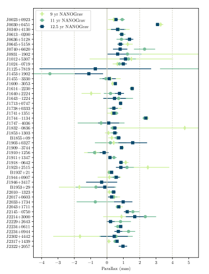
Figure 3: Parallax measurements and formal uncertainties for all 12.5-year pulsars from NG9, NG11, and the current data set. While only values of parallax greater than zero are physically meaningful, all formally fit values are shown here; the preponderance of positive values serves to verify that a real physical parameter is being measured. Two outlier values from previous data releases fall beyond the right edge of the plot, as indicated by the error bars.

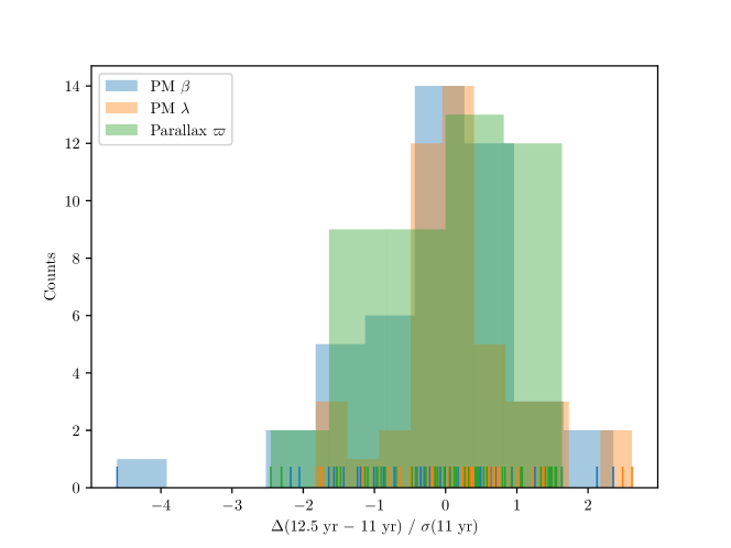
Figure 4: Comparison of astrometric measurements across NG11 and the current 12.5-year data set. The differences in proper motion ($\mu_{\beta},\;\mu_{\lambda}$) and parallax $\varpi$ are shown in units of the uncertainty in the 11-year measurement ($\sigma_{11}$). The figure shows binned histograms of each type of measurement, with all individual measurements superimposed as short vertical lines at the bottom of the figure. The value of $\mu_{\beta}$ for PSR J2214+3000 is an outlier at $-4.6\,\sigma$; the rest are reasonably consistent, as discussed in the text.

As noted previously, our pulsar timing analyses always include five astrometric parameters as free parameters: two sky position parameters, two components of proper motion, and annual trigonometric parallax. Detailed analyses of the astrometry of NANOGrav pulsars, including comparisons with VLBI measurements, were presented in Matthews et al. (2016) and NG11, thus we do not repeat such a detailed analysis in the present work. Comparisons of astrometric measurements obtained via different measurement methods (e.g., table 5) are potentially useful for such purposes as tying astrometric reference frames (Wang et al., 2017), using measurements made by one method as priors in analysis of other data, etc. To make use of pulsar astrometric measurements, it is important that they be robust, accurate, and stable over time. To test the stability of our astrometric measurements, we compare the parallax and proper motion measurements between the current and previous NANOGrav data releases (with newly-detected astrometric parameters specifically highlighted in the previous section).

For pulsar timing, the position (and hence proper motion) is naturally parameterized in terms of ecliptic coordinates. As the timing data span increases, the proper motion is expected to be measured with increasing accuracy, and the covariance between proper motion and parallax should rapidly decrease. Figure 3 shows the measured parallaxes in the 12.5-year data release, as well as previous (NG9 and NG11) measurements, where available. The number of measurements has increased (see Section 5.1 below) and the formal significance has generally improved.

However, a comparison of the changes in astrometric parameters between the current and previous (11-year) data releases might suggest that some caution is warranted. In Figure 4 we show histograms of the differences in proper motion ($\mu_{\beta}$ and $\mu_{\lambda}$) and parallax ($\varpi$) between the current (12.5-year) and NG11 data releases, with the differences scaled by the estimated uncertainty for the 11-year parameters (i.e., $(P_{12.5}-P_{11})/\sigma_{11}$, where $P=\{\mu_{\beta},\mu_{\lambda},\varpi\}$).

The single obvious outlier is the measurement of $\mu_{\beta}$ for PSR J2214$+$3000, at $-4.6\sigma_{11}$. For pulsars near the ecliptic plane, the ecliptic latitude $\beta$ is poorly constrained by timing in comparison to the ecliptic longitude $\lambda$, and we expect the accuracy of $\mu_{\beta}$ measurements to be correspondingly worse. That alone cannot explain the discrepancy for J2214$+$3000, at $\beta=37.7\arcdeg$. The other notable fact about this source is that it is one of four black widow pulsars in our data set, along with J0023$+$0923, J0636$+$5128, and J2234$+$0944. Like the other black widows in our sample, it does not exhibit eclipses (Ransom et al., 2011), and, as with J2234$+$0944, it does not show orbital variability (Bak Nielsen et al., 2020; Arzoumanian et al., 2018a). In NG11, we noted difficulty fitting a noise model to this pulsar, possibly related to excess noise in mid-to-late 2013. Imperfect noise modeling, combined with covariance between noise parameters and astrometric parameters, may contribute to the change in reported $\mu_{\beta}$ value.

Besides J2214$+$3000, the astrometric parameters appear generally consistent between the 11-year and 12.5-year measurements, with $\sim$85% of the measurements differing by less than $\pm 1.5\,\sigma_{11}$. Even though NG11 is a subset of the 12.5-year data release, such measurement differences are not unreasonable. Due to the additional processing of the 12.5-year data, as described in Section 2.5, in combination with a longer baseline that further down-weights the earlier, less constraining data, such changes in the astrometric parameters can be expected.

7 Binary Analysis of Selected Pulsars

In NG11, we presented a summary of modeling methods and results for binary pulsars in the data set presented therein; we do not repeat such detailed descriptions here. Instead, we highlight five binary pulsars for which additional description or analysis is warranted. PSR J0740+6620 is an extremely high-mass MSP for which a more up-to-date timing solution is published in Cromartie et al. (2020); for PSRs J1909$-$3744 and J2234+0611, significant testing was required to obtain the timing models presented in this work; and we use the newly-measured Shapiro delay parameters of PSRs J1853+1303 and J2145$-$0750 to place mass and geometry constraints on these systems.

7.1 PSR J0740+6620

In the course of analyzing the 12.5-yr data set, we found that the significance of the Shapiro delay in PSR J0740+6620 had dramatically increased from its initial detection in NG11. The constraints on $m_{\rm c}$, $\sin i$, and the pulsar mass ($m_{\rm p}$) from the nominal 12.5-yr data set motivated additional, targeted observations for improving the Shapiro-delay measurement. By combining 12.5-yr NANOGrav timing data with additional data obtained during specific orbital phases optimally sensitive to Shapiro delay, Cromartie et al. (2020) found an improved pulsar mass of $m_{\rm p}=2.14^{+0.10}_{-0.09}\textrm{ M}_{\odot}$ (68.3% credible region), representing the most massive, precisely-measured neutron star known to date.

7.2 PSR J1853+1303

Both $h_{3}$ and $h_{4}$ of the orthometric parameterization of the Shapiro delay (Freire & Wex, 2010) for PSR J1853+1303 are significant. Our new measurements ($h_{3}=0.18\pm 0.04\,\mu$s, $h_{4}=0.17\pm 0.05\,\mu$s) are consistent with those first presented in NG11. We tested whether $\sin{i}$ and $m_{c}$ could be independently measured using Tempo, as described in Section 3.1, but this test was not successful.

The orthometric parameters $h_{3}$, $h_{4}$, and $\varsigma$ are related to the traditional post-Keplerian Shapiro delay parameters as:

$$\varsigma =\sqrt{\frac{1-\cos{i}}{1+\cos{i}}}$$ (3)

$$h_{3} =r\varsigma^{3}$$ (4)

$$h_{4} =h_{3}\varsigma$$ (5)

where $r=m_{\mathrm{c}}T_{\odot}$ is the “range” of the delay, $m_{\mathrm{c}}$ is the companion mass, and $T_{\odot}\simeq 4.93\,\mu$s. This parameterization constrains the orbital inclination to $i=85^{\circ}\pm 14^{\circ}$ (we quote the $1\sigma$ uncertainty, derived from error propagation beginning with the $1\sigma$ parameter uncertainties from the Tempo timing model). The orthometric parameters are not yet sufficiently well-measured to place meaningful bounds on $r$ and, therefore, the companion mass, which we calculate to be consistent with zero (at the $1\sigma$ confidence level). More insight into the physical properties of this system may be gained by explicit gridding of the posterior distribution in future work.

7.3 PSR J1909$-$3744

The value of $\dot{x}$ for PSR J1909$-$3744 has been measured or constrained by several groups. Verbiest et al. (2009) found $\dot{x}=(5\pm 4)\times 10^{-16}$ lt-s s^-1, while Desvignes et al. (2016) found $\dot{x}=(0.6\pm 1.7)\times 10^{-16}$ lt-s s^-1. In NG11, we found $\dot{x}=(-4\pm 1)\times 10^{-16}$ lt-s s^-1. Using the 12.5-yr data set for PSR J1909$-$3744, we have further constrained its value to $(-2.9\pm 0.8)\times 10^{-16}$ lt-s s^-1.

As in NG9 and NG11, we detect red noise in PSR J1909$-$3744. In this work, we find $\dot{x}$ and the red-noise terms in the timing model to be covariant. In particular, the presence or absence of $\dot{x}$ in the timing model had a significant effect on the red noise amplitude: the amplitude was significantly lower when $\dot{x}$ was included in the model, compared to when $\dot{x}$ was not included. Additionally, if $\dot{x}$ was initially excluded from the timing model such that the red noise amplitude assumed its higher value, then adding $\dot{x}$ to the model while red noise was also included resulted in a non-measurement of $\dot{x}$ according to our $F$-test criterion. While not common, this covariant behavior is not unexpected, as $\dot{x}$ is a secular parameter that evolves slowly, as does red noise.

The value of $\dot{x}$ can be inferred from the changing geometry due to the relative motion between the pulsar system and Earth (Kopeikin, 1995),

$$\dot{x}_{\mathrm{k}}=x\mu\cot{i}\sin{(\Theta_{\mu}-\Omega)}$$ (6)

where $\sin i$ is constrained from the Shapiro delay, giving $i=86.39^{\circ}$ or $93.61^{\circ}$; the magnitude of proper motion $\mu=36.94$ mas yr^-1; the position angle of the proper motion ($\Theta_{\mu}$) is derived from timing measurements of proper motion; and $\Omega$ is the longitude of the ascending node. In the case where annual orbital parallax is detected, the three-dimensional geometry of the system can be constrained, such that the values of $i$ and $\Omega$ are measured definitively (as opposed to having two possible values of $i$ and four possible values of $\Omega$).

We attempted to directly fit for $i$ and $\Omega$ using the DDK model in Tempo, but the fit did not converge. Therefore, we instead performed the following test to determine whether we were likely measuring a physically reasonable value of $\dot{x}$ in the absence of a significant detection of annual orbital parallax. Using the T2 model in Tempo2 we found the best-fit $(i,\Omega)=\{(86.39^{\circ},350^{\circ}),(93.61^{\circ},170^{\circ})\}$, and used them to calculate $\dot{x}_{\mathrm{k}}$. In all cases, $\dot{x}_{\mathrm{k}}\approx-3\times 10^{-16}$ lt-s s^-1, consistent with the value we measure from timing.

This result suggests that the $\dot{x}$ we measure with Tempo for PSR J1909$-$3744 is robust, and should be included in the model rather than being absorbed by red noise. As noted above, it is also consistent with and an improvement upon our $\dot{x}$ measurement from NG11. We have therefore included this $\dot{x}$ value in our timing model for this pulsar.

7.4 PSR J2145$-$0750

We can place loose constraints on the geometry of the PSR J2145$-$0750 system using the proper motion and $h_{3}$ measurements. An upper bound on the orbital plane inclination can be calculated by inverting equation 6 and attributing the measured $\dot{x}$ to the proper motion (e.g., Fonseca et al., 2016):

$$i_{\mathrm{max}}=\arctan\frac{x\mu}{|\dot{x}_{\mathrm{obs}}|},$$ (7)

yielding $i_{\mathrm{max}}=74^{\circ}\pm 5^{\circ}$. We can then combine equations 3 and 4 to obtain $r_{\mathrm{min}}$, yielding a lower bound on the companion mass, $m_{\mathrm{c,min}}=r_{\mathrm{min}}/T_{\odot}=0.08\pm 0.03\,M_{\odot}$. Much more robust system constraints have previously been made with a combination of optical imaging, VLBI parallax, and radio timing: $i=21^{+7}_{-4}$ degrees and $m_{\mathrm{c}}=0.83\pm 0.06\,M_{\odot}$ (Deller et al., 2016), and $i=34^{+5}_{-7}$ degrees and $m_{\mathrm{p}}=1.3^{+0.4}_{-0.5}\,M_{\odot}$ (Fonseca et al., 2016). We will place improved constraints on the geometry and mass of the PSR J2145$-$0750 system in future studies with longer timing baselines.

7.5 PSR J2234+0611

The eccentric orbit and high timing precision of J2234+0611 allowed Stovall et al. (2019) to measure a large number of binary-related effects from this system, including one orthometric Shapiro delay parameter ($h_{3}$) and annual orbital parallax. Together, these measurements allowed Stovall et al. to unambiguously determine the three-dimensional geometry of the system, giving $i\approx 138.7^{\circ}$ and $\Omega\approx 44^{\circ}$. These parameters correspond to $\dot{x}_{\mathrm{k}}=(-2.78\pm 0.07)\times 10^{-14}$ lt-s s^-1.

In this work, we find that $i$ and $\Omega$ are not constrained, and we do not obtain a significant measurement of $h_{3}$. There are two likely reasons that we are not able to reproduce the measurements of Stovall et al. First, their data set is a superset of that presented here, with an additional $\sim 1.5$ yr in their timing baseline. Secondly, Stovall et al. fix $i$ and $\varsigma=h_{4}/h_{3}$ based on the derived value of $s=\sin{i}$ from the DDGR binary model; they then constrain $\Omega$ by running Tempo over a grid in $i$, $\Omega$, and $m_{\mathrm{tot}}=m_{\rm p}+m_{\rm c}$, where $i$ and $\Omega$ are held constant at each step. Based on our $F$-test criterion for including post-Keplerian parameters, we instead fit for $\dot{x}$ (which is related to annual orbital parallax and its secular variation shown in Equation 6); its value, $(-2.8\pm 0.2)\times 10^{-14}$ lt-s s^-1, is consistent with that found by Stovall et al.

8 Flux Densities

The algorithm used to calculate TOAs in our narrowband data (Section 2.4) also yields the amplitudes of the pulsed signals relative to the amplitudes of the template profiles used for timing. Through suitable calibration and normalization of the template profiles, these amplitudes can be used to estimate the period-averaged flux densities of the pulsed signals. In this section, we describe our flux density calculations. The results are summarized in Table 6.

For the flux density analysis, we used only GUPPI and PUPPI data. The narrower bands of GASP and ASP made them less suitable for the cross-checks described below and would have yielded less robust measurements.

Table 6: Flux densities

PSR	Obs.		$S_{430}$				$S_{800}$				$S_{1400}$				$S_{2000}$				Spectral
				(mJy)				(mJy)				(mJy)				(mJy)			Index
			16	50	84		16	50	84		16	50	84		16	50	84
J0023$+$0923	AO		01.93	02.50	03.95		$\cdots$	$\cdots$	$\cdots$		00.21	00.32	00.54		$\cdots$	$\cdots$	$\cdots$		$-1.74$
J0030$+$0451	AO		02.34	05.80	23.12		$\cdots$	$\cdots$	$\cdots$		00.85	01.12	01.60		00.48	00.60	00.78		$-1.39$
J0340$+$4130	GB		$\cdots$	$\cdots$	$\cdots$		01.14	01.42	01.89		00.45	00.54	00.60		$\cdots$	$\cdots$	$\cdots$		$-1.73$
J0613$-$0200	GB		$\cdots$	$\cdots$	$\cdots$		05.45	06.66	08.12		01.81	02.17	02.48		$\cdots$	$\cdots$	$\cdots$		$-2.00$
J0636$+$5128	GB		$\cdots$	$\cdots$	$\cdots$		01.64	02.08	02.90		00.73	00.94	01.18		$\cdots$	$\cdots$	$\cdots$		$-1.42$
J0645$+$5158	GB		$\cdots$	$\cdots$	$\cdots$		00.47	00.76	02.02		00.17	00.29	00.86		$\cdots$	$\cdots$	$\cdots$		$-1.72$
J0740$+$6620	GB		$\cdots$	$\cdots$	$\cdots$		01.11	02.19	06.06		00.43	00.97	01.71		$\cdots$	$\cdots$	$\cdots$		$-1.46$
J0931$-$1902	GB		$\cdots$	$\cdots$	$\cdots$		01.41	01.90	02.60		00.60	00.84	01.24		$\cdots$	$\cdots$	$\cdots$		$-1.46$
J1012$+$5307	GB		$\cdots$	$\cdots$	$\cdots$		03.19	06.93	16.46		01.46	02.90	06.09		$\cdots$	$\cdots$	$\cdots$		$-1.56$
J1024$-$0719	GB		$\cdots$	$\cdots$	$\cdots$		01.43	02.92	07.48		00.74	01.36	02.56		$\cdots$	$\cdots$	$\cdots$		$-1.37$
J1125$+$7819	GB		$\cdots$	$\cdots$	$\cdots$		01.39	02.58	05.20		00.55	00.90	01.70		$\cdots$	$\cdots$	$\cdots$		$-1.88$
J1453$+$1902	AO		01.11	01.64	02.81		$\cdots$	$\cdots$	$\cdots$		00.11	00.17	00.48		$\cdots$	$\cdots$	$\cdots$		$-1.92$
J1455$-$3330	GB		$\cdots$	$\cdots$	$\cdots$		01.42	02.28	05.03		00.45	00.73	01.51		$\cdots$	$\cdots$	$\cdots$		$-2.04$
J1600$-$3053	GB		$\cdots$	$\cdots$	$\cdots$		02.66	03.17	04.02		01.99	02.37	02.99		$\cdots$	$\cdots$	$\cdots$		$-0.52$
J1614$-$2230	GB		$\cdots$	$\cdots$	$\cdots$		02.02	02.68	03.51		00.79	01.11	01.53		$\cdots$	$\cdots$	$\cdots$		$-1.58$
J1640$+$2224	AO		04.20	06.31	11.33		$\cdots$	$\cdots$	$\cdots$		00.24	00.54	01.26		$\cdots$	$\cdots$	$\cdots$		$-2.08$
J1643$-$1224	GB		$\cdots$	$\cdots$	$\cdots$		11.31	13.02	14.50		04.06	04.70	05.38		$\cdots$	$\cdots$	$\cdots$		$-1.82$
J1713$+$0747	AO		$\cdots$	$\cdots$	$\cdots$		$\cdots$	$\cdots$	$\cdots$		02.47	04.69	08.70		02.24	05.01	10.24		+$0.19$
J1713$+$0747	GB		$\cdots$	$\cdots$	$\cdots$		03.39	06.14	12.12		02.02	04.32	08.43		$\cdots$	$\cdots$	$\cdots$		$-0.63$
J1738$+$0333	AO		$\cdots$	$\cdots$	$\cdots$		$\cdots$	$\cdots$	$\cdots$		00.37	00.48	00.82		00.26	00.43	00.65		$-0.31$
J1741$+$1351	AO		01.79	02.60	04.64		$\cdots$	$\cdots$	$\cdots$		00.14	00.21	00.38		$\cdots$	$\cdots$	$\cdots$		$-2.13$
J1744$-$1134	GB		$\cdots$	$\cdots$	$\cdots$		02.94	05.29	10.48		00.98	01.96	04.74		$\cdots$	$\cdots$	$\cdots$		$-1.77$
J1747$-$4036	GB		$\cdots$	$\cdots$	$\cdots$		05.63	06.85	09.05		01.31	01.55	02.20		$\cdots$	$\cdots$	$\cdots$		$-2.66$
J1832$-$0836	GB		$\cdots$	$\cdots$	$\cdots$		03.14	03.65	04.23		00.90	01.11	01.35		$\cdots$	$\cdots$	$\cdots$		$-2.13$
J1853$+$1303	AO		03.13	04.71	07.11		$\cdots$	$\cdots$	$\cdots$		00.24	00.43	00.59		$\cdots$	$\cdots$	$\cdots$		$-2.03$
B1855$+$09	AO		14.36	19.17	26.18		$\cdots$	$\cdots$	$\cdots$		02.13	03.47	06.50		$\cdots$	$\cdots$	$\cdots$		$-1.45$
J1903$+$0327	AO		$\cdots$	$\cdots$	$\cdots$		$\cdots$	$\cdots$	$\cdots$		00.63	00.69	00.79		00.45	00.52	00.58		$-0.79$
J1909$-$3744	GB		$\cdots$	$\cdots$	$\cdots$		01.54	03.01	05.15		00.55	01.03	02.17		$\cdots$	$\cdots$	$\cdots$		$-1.92$
J1910$+$1256	AO		$\cdots$	$\cdots$	$\cdots$		$\cdots$	$\cdots$	$\cdots$		00.35	00.56	00.69		00.21	00.31	00.47		$-1.66$
J1911$+$1347	AO		02.10	02.93	04.16		$\cdots$	$\cdots$	$\cdots$		00.51	00.86	01.26		$\cdots$	$\cdots$	$\cdots$		$-1.04$
J1918$-$0642	GB		$\cdots$	$\cdots$	$\cdots$		03.12	04.13	05.43		00.89	01.36	01.99		$\cdots$	$\cdots$	$\cdots$		$-1.98$
J1923$+$2515	AO		02.04	02.56	03.36		$\cdots$	$\cdots$	$\cdots$		00.18	00.28	00.49		$\cdots$	$\cdots$	$\cdots$		$-1.87$
B1937$+$21	AO		$\cdots$	$\cdots$	$\cdots$		$\cdots$	$\cdots$	$\cdots$		09.14	12.44	16.56		03.24	04.72	06.25		$-2.72$
B1937$+$21	GB		$\cdots$	$\cdots$	$\cdots$		41.93	56.37	74.68		11.33	14.83	18.65		$\cdots$	$\cdots$	$\cdots$		$-2.39$
J1944$+$0907	AO		14.57	18.82	28.53		$\cdots$	$\cdots$	$\cdots$		01.08	01.94	03.41		$\cdots$	$\cdots$	$\cdots$		$-1.92$
J1946$+$3417	AO		$\cdots$	$\cdots$	$\cdots$		$\cdots$	$\cdots$	$\cdots$		00.84	00.92	00.96		00.56	00.61	00.66		$-1.15$
B1953$+$29	AO		10.77	12.00	13.28		$\cdots$	$\cdots$	$\cdots$		00.69	00.94	01.21		$\cdots$	$\cdots$	$\cdots$		$-2.16$
J2010$-$1323	GB		$\cdots$	$\cdots$	$\cdots$		01.20	01.63	02.12		00.50	00.71	00.92		$\cdots$	$\cdots$	$\cdots$		$-1.49$
J2017$+$0603	AO		$\cdots$	$\cdots$	$\cdots$		$\cdots$	$\cdots$	$\cdots$		00.22	00.32	00.46		00.21	00.31	00.42		$-0.09$
J2033$+$1734	AO		02.98	03.62	04.23		$\cdots$	$\cdots$	$\cdots$		00.26	00.30	00.38		$\cdots$	$\cdots$	$\cdots$		$-2.11$
J2043$+$1711	AO		01.51	01.99	03.01		$\cdots$	$\cdots$	$\cdots$		00.15	00.21	00.40		$\cdots$	$\cdots$	$\cdots$		$-1.91$
J2145$-$0750	GB		$\cdots$	$\cdots$	$\cdots$		05.10	14.25	38.84		01.69	04.86	12.15		$\cdots$	$\cdots$	$\cdots$		$-1.92$
J2214$+$3000	AO		$\cdots$	$\cdots$	$\cdots$		$\cdots$	$\cdots$	$\cdots$		00.28	00.38	00.70		00.20	00.35	00.51		$-0.23$
J2229$+$2643	AO		02.19	03.61	07.96		$\cdots$	$\cdots$	$\cdots$		00.22	00.41	00.70		$\cdots$	$\cdots$	$\cdots$		$-1.84$
J2234$+$0611	AO		00.72	00.90	01.82		$\cdots$	$\cdots$	$\cdots$		00.12	00.33	00.89		$\cdots$	$\cdots$	$\cdots$		$-0.85$
J2234$+$0944	AO		$\cdots$	$\cdots$	$\cdots$		$\cdots$	$\cdots$	$\cdots$		00.81	01.15	02.83		00.40	00.76	01.14		$-1.16$
J2302$+$4442	GB		$\cdots$	$\cdots$	$\cdots$		02.59	03.29	04.31		01.06	01.41	01.84		$\cdots$	$\cdots$	$\cdots$		$-1.51$
J2317$+$1439	AO		04.81	07.20	09.96		$\cdots$	$\cdots$	$\cdots$		00.26	00.45	00.80		$\cdots$	$\cdots$	$\cdots$		$-2.35$
J2322$+$2057	AO		01.37	01.94	03.54		$\cdots$	$\cdots$	$\cdots$		00.14	00.26	00.72		00.31	00.32	01.06		$-1.70$

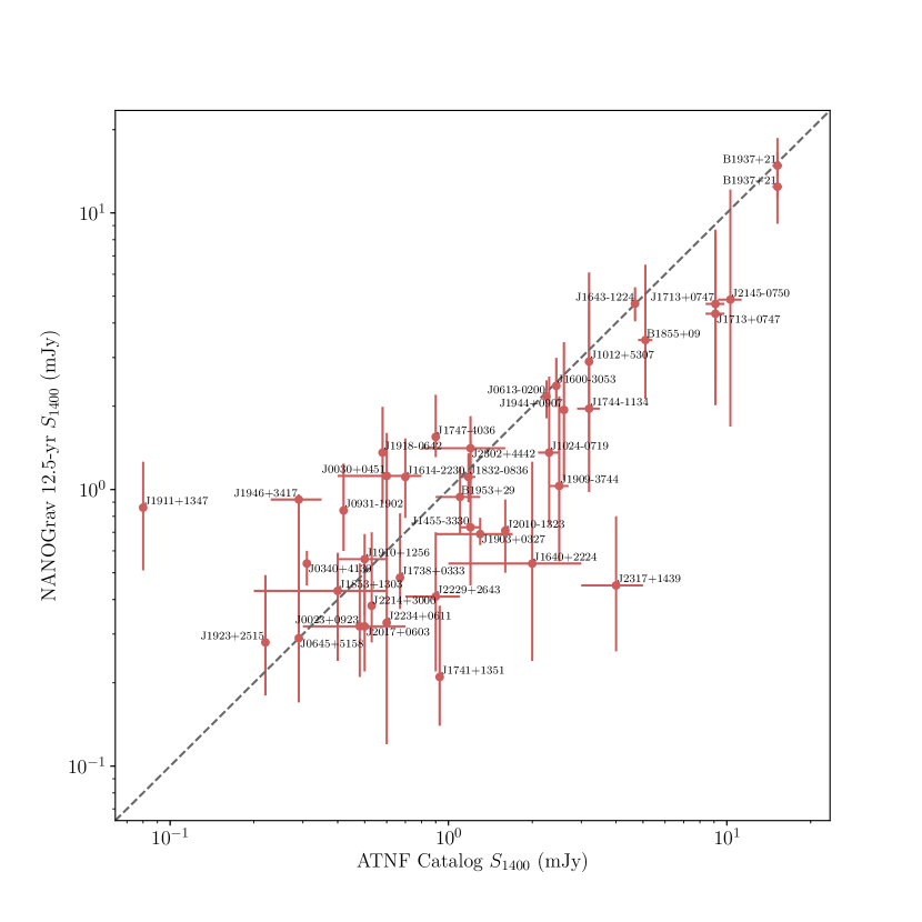
Figure 5: Comparison of 1400 MHz flux density measurements ($S_{\rm 1400}$) from the present paper (vertical axis) with values in the ATNF pulsar catalog (horizontal axis; Manchester et al., 2005, version 1.63). Vertical error bars indicate the central 68% of measured flux density values (Table 6). Horizontal error bars, where present, indicate the uncertainties reported in the ATNF pulsar catalog. Two pulsars are shown twice (J1713+0747 and B9137+21), with similar values, because we made separate analyses of our Arecibo and GBT measurements.

Table 7: Comparison of Spectral Indexes

PSR	Obs.		NG12.5		Frail et al. (2016)
			$\alpha$		$\alpha$	$\sigma_{\alpha}$
J0030$+$0451	AO		-1.39		-1.93	0.15
J1643$-$1224	GB		-1.82		-1.64	0.06
J1747$-$4036	GB		-2.66		-2.81	0.22
B1937$+$21	AO		-2.72		-2.51	0.17
B1937$+$21	GB		-2.39		-2.51	0.17
J1944$+$0907	AO		-1.92		-3.03	0.06
B1953$+$29	AO		-2.16		-1.77	0.09
J2145$-$0750	GB		-1.92		-1.47	0.61
J2317$+$1439	AO		-2.35		-0.86	0.12

8.1 Absolute Calibration

As described in Section 2, each individual observation was preceded by a pulsed-cal measurement using an artificial noise signal. The pulsed-cal measurements were used to calibrate the amplitude scale of the pulsar observations. The noise signals themselves were calibrated by measuring them in on- and off-source observations of a standard continuum calibrator radio source. The noise signals were checked against the continuum calibrator approximately once per month at each observatory. Thus our flux density measurements depend directly on our assumptions about the continuum calibrator flux density.

For continuum calibration, we used the compact radio source J1445+0958 (B1442+101) for all GUPPI observations and all PUPPI observations after MJD 56619 (2013 November 29). We only used data calibrated with this source in the flux density analysis. The VLA calibrator manual gives the flux density of J1445+0958 as 2.60, 1.20, 0.73 0.40, and 0.10 Jy at wavelengths of 20.0, 6.0, 3.7, 2.0, and 0.7 cm, respectively. We modeled this using the analytic expression $\log S=\sum_{i=0}^{3}a_{i}\left(\log\nu_{\rm GHz}\right)^{i}$, where $\nu_{\rm GHz}$ is the radio frequency in gigahertz and the coefficients for J1445+0958 are $a_{0}=0.389314$, $a_{1}=-0.0280647$, $a_{2}=-0.600809$, and $a_{3}=0.0262127$.

8.2 Data Checks and Cleaning

Flux density measurements are particularly susceptible to calibration errors, so we undertook further checks of the data used for this purpose.

The signal-to-noise ratio of a pulsar observation is expected to be ${\rm S/N}=SG/T_{\rm sys}\sqrt{2Bt}\sqrt{(P-w)/w}$, where $S$, $G$, $T_{\rm sys}$, $B$, $t$, $P$, and $w$ are the pulsar flux, telescope gain, system temperature, bandwidth, observing time, pulse period, and pulse width, respectively, and where $\sqrt{(P-w)/w}$ is a proxy for a general pulse-shape-dependent factor. For a given telescope, receiver, and pulsar, at a given radio frequency, the ratio $(S/[{\rm S/N}])\sqrt{2Bt}$ should be constant (after considering small variations due to radiometer noise and variations in $G$ and $T_{\rm sys}$ due to telescope elevation). Radio-frequency interference, calibration errors, and other defects in the data can cause this ratio to vary. We used this to flag potentially discrepant flux density values. We removed any data point for which this ratio was less than 0.75 or more than 1.75 times the median value for that frequency and nearby frequencies at low S/N, with a gradually increasing allowed upper value for high S/N (analyzed over ranges of 100 MHz above 1 GHz, 50 MHz for the GBT 820 MHz receiver, and 10 MHz for the Arecibo 327 and 430 MHz receivers). At $\nu>2300$ MHz, we used a lower limit on the ratio of 0.50 rather than 0.75. Further, we entirely eliminated any observation for which five or more individual flux values were flagged as potentially discrepant. These specific choices were based on empirical analysis of the data. They eliminated obvious outliers while allowing us to retain most of the flux density measurements.

8.3 Flux Density Measurement Results

For each epoch, we fit the observed set of narrowband flux values to a power law, $S_{\rm obs}(\nu)=S_{\nu_{0}}(\nu/\nu_{0})^{\alpha}$. Here $S_{\nu_{0}}$ is the fit flux at fiducial frequency $\nu_{0}$ and $\alpha$ is the spectral index. We used fiducial frequencies of 430, 800, 1400, and 2000 MHz, chosen for their locations near the centers of the observing bands and, in some cases, because they are standard frequencies used in pulsar catalogs. We calculated separate values of $S_{\nu_{0}}$ and $\alpha$ for each receiver at each observing epoch (defined as observations within a 3-day span).

For most pulsars, the values of $\alpha$ within these single-receiver, single-epoch fits varied widely due to diffractive scintillation within the receiver bands; we do not use those values further.

Table 6 reports the median observed flux density for each pulsar and each receiver, along with 16th and 84th percentile values. The table also includes spectral indexes calculated using the median flux density values in two bands (as specified in the table). For the two pulsars observed at both Arecibo and GBT (PSRs J1713+0747 and B1937+21), we analyzed the measurements from the observatories separately as a check against systematic errors. Their $S_{1400}$ measurements show good agreement between the two observatories.

PSR J1713+0747 shows a significant difference between the spectral index calculated from Arecibo values of $S_{1400}$ and $S_{2000}$ and the spectral index calculated from GBT values of $S_{800}$ and $S_{1400}$. This suggests that a single power law is not sufficient to model the flux density across a wide range of frequencies. PSR B1937+21 also shows a difference in spectral indexes between the two observatories, albeit somewhat smaller (and in the opposite direction) than that of J1713+0747.

Because our flux density analysis only includes measurements from observations that yielded good narrowband TOA values, it excludes observations in which the pulsar had a very low S/N or was not visible at all. This could potentially bias our measurements high (since low flux density values due to, e.g., extreme scintillation are excluded). Furthermore, we used a constant template profile for the narrowband TOA measurements, which assumes that the true profile shape does not evolve with frequency across the band; the amplitude, and thus the estimated flux density, will depend on the degree to which this assumption holds. We believe both of these factors only have a small effect in our reported measurements, but a detailed analysis of these biases is beyond the scope of the present work.

The spectral indexes of sources observed at Arecibo at 1400 and 2000 MHz tend to have smaller magnitudes than the spectral indexes of other pulsars. This is almost certainly a selection effect. We preferentially observe Arecibo pulsars with this combination of receivers, but only when the pulsar is strong enough to be consistently detected with high signal-to-noise at 2000 MHz. This implies that such sources have relatively high flux densities at 2000 MHz, and therefore relatively shallow spectra.

8.4 Comparison with Previous Work

A comparison between our $S_{1400}$ measurements and previously reported values for 41 pulsars is given in Figure 5. There is some scatter in the values, likely attributable to scintillation-induced variations in flux density measurements, particularly in previous measurements which might be based on a small number of samples. The median ratio of $S_{1400}$ from our measurements to the $S_{1400}$ of previous measurements was 0.82, and the average value of this ratio was 1.19. The latter is evidently dominated by a few sources with the most significant discrepancies. The most significant outlier values are for PSR J1911+1347, for which we report median $S_{1400}=0.86$ mJy, while the previous reported value was 0.08 mJy, more than an order of magnitude lower (Lorimer et al., 2006); and for PSR J2317+1439, for which we report median $S_{1400}=0.45$ mJy, while the previous reported value was $4\pm 1$ mJy, more than an order of magnitude greater (Kramer et al., 1998). The reason for the relatively large discrepancies in reported values for these two pulsars is not known.

We made similar comparisons between our flux density measurements and cataloged values at 430 MHz (11 pulsars) and 2000 MHz (1 pulsar). The results were comparable to those at 1400 MHz: general agreement with modest scatter between new and previous measurements.

Shaifullah (2017, herein S2017) reports measurements of spectral indexes of a dozen MSPs at Arecibo using the 327 MHz and 1400 MHz receivers. Of those, five MSPs were observed for a large number of epochs (thus mitigating scintillation issues). Within that group, two overlap with the present work, and both show good agreement with our measurements: For PSR J1453+1902, we find $\alpha=-1.92$, and S2017 reports $\alpha=-1.7\pm 0.4$; for J2322+2057, we find $\alpha=-1.70$, and S2017 reports $\alpha=-1.7\pm 0.1$. (Other pulsars in S2017 with fewer observations show larger discrepancies.)

Frail et al. (2016) reported spectral indexes of many pulsars calculated by combining Giant Metrewave Radio Telescope (GMRT) 150 MHz observations with measurements in the literature at other frequencies. A summary is presented in Table 7, which lists the spectral indexes from the present work (NG12.5), along with the spectral indexes and their uncertainties, $\sigma_{\alpha}$ reported by Frail et al. (2016). Many measurements are in agreement, but a few are not. It is not clear whether this is because of differences in observing frequency (and the possible inadequacy of a single power-law to describe flux density) or whether it is caused by something else.

9 Summary and Conclusions

In this paper, we have introduced the NANOGrav 12.5-year data set, which contains TOAs and timing models for 47 MSPs with baselines between $\sim 2$ and $\sim 13$ years (Section 2). In particular, the present work follows in the footsteps of NANOGrav’s preceding three data releases (NG5, NG9, and NG11). We have given the TOAs discussed in this paper the designation “narrowband” to distinguish them from the “wideband” data set that uses a number of new developments to process the same pulse profile data (see the parallel paper, Alam et al., 2020).

These data introduced two new pulsars into our PTA (PSRs J1946$+$3417 and J2322$+$2057) and extended our baseline by 1.5 years. A number of new procedural changes and quality control measures were introduced over NG11. In addition to the wideband processing, for this data set we:

1. Removed low-amplitude artifact images from the profile data that were introduced by the interleaved samplers of the ADCs (Section 2.3).

2. Automated and systematized the timing analysis procedure with Jupyter notebooks (Section 3).

3. Excised whole epochs of data based on their disproportionately large influence on timing fit $\chi^{2}$, as indicated by an $F$-test (Section 2.5).

4. Identified and excised specious TOAs by examining calibration scans and flux densities (Section 2.5).

5. Introduced -cut flags that document why a TOA has been removed from the data set (Section 2.5).

6. Transitioned to the ENTERPRISE PTA analysis software for noise modeling (Section 3.3).

7. Cross-checked timing results with the new, Tempo- and Tempo2-independent pulsar timing software PINT (Section 4).

8. Included per-TOA flux density measurements (Section 8).

Some of these changes led to improvements in the white noise model parameters, as indicated by a re-analysis of the data in NG11 compared to the 11-year “slice” of the present data set (Section 3.4). The red noise detected in eleven sources in NG11 continues to be present (Section 3.3). Red noise is also detected in an additional three pulsars—PSRs J1744$-$1134, J1853$+$1303, and J2317$+$1439—the first and third of which are bright, precisely timed pulsars with some of the longest baselines in the data set. A number of other pulsars have sub-threshold hints of red noise, which may become significant in future data sets.

Two of the main astrophysical results from this data set—the observation of a second chromatic ISM event in PSR J1713$+$0747 (Lam et al., 2018b), and the discovery that PSR J0740$+$6620 is the most massive, precisely-measured neutron star known to date (Cromartie et al., 2020)—were published prior to the present work. Additionally, the entire data set was analyzed for pulse phase jitter in Lam et al. (2019); Deneva et al. (2019) used data from this release to compare the radio timing stability of PSR B1937$+$21 with that seen by the NICER X-ray instrument; and Stovall et al. (2019) used a superset of these observations to solve the 3-D orbit of PSR J2234$+$0611. In Section 5 we highlighted a number of other new NANOGrav measurements, which include the first published measurements of trigonometric parallax for PSRs J1832$-$0836 and J2322$+$2057, of $\dot{x}$ for J0613$-$0200 and J2229+2643, and of $h_{3}$ indicating a marginally-detected Shapiro delay in J2145$-$0750.

NANOGrav is committed to continued public data releases, both for individual studies of high-precision pulsar timing and for the sake of gravitational wave detection. Analyses of these data to model a variety of gravitational wave signals will be presented in forthcoming publications, with our latest results from searching for a stochastic background presented in Arzoumanian et al. (2020). Furthermore, advanced noise modeling techniques in which bespoke models are applied to each pulsar are anticipated to further increase our sensitivity, and will also be presented elsewhere (Simon et al., 2020, in preparation). Increasing the number of pulsars in the array has the largest impact on determining the prospects for detection of the stochastic background. To this end, we are already synthesizing our next data set, which will come with the single largest increase in the number of pulsars ($\sim$50%) since we doubled the size of the array between NG5 and NG9. The concomitant increase in the sensitivity and complexity of our PTA analyses promises to deliver an exciting upcoming few years of nanohertz gravitational wave astrophysics.

Appendix A Averaged Residuals

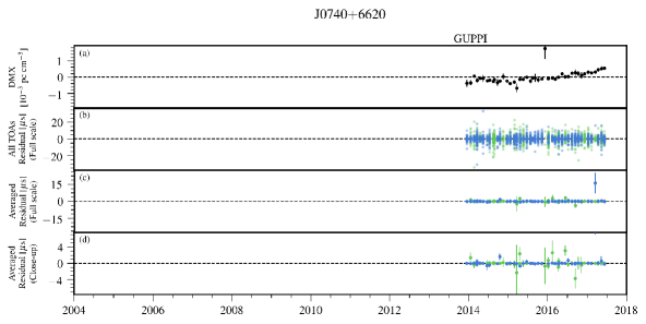
Figure 12: Timing residuals and DM variations for PSR J0740$+$6620. See appendix A text for details. In residual plots, colored points indicate the receiver of each observation: 820 MHz (Green) and 1.4 GHz (Dark blue). (a) Variations in DMX. (b) Residual arrival times for all TOAs. Points are semi-transparent; dark regions arise from the overlap of many points. (c,d) Average residual arrival times shown full scale (panel c) and close-up of low residuals (panel d).

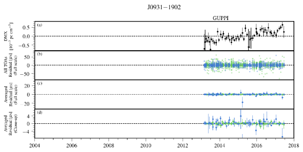
Figure 13: Timing residuals and DM variations for PSR J0931$-$1902. See appendix A text for details. In residual plots, colored points indicate the receiver of each observation: 820 MHz (Green) and 1.4 GHz (Dark blue). (a) Variations in DMX. (b) Residual arrival times for all TOAs. Points are semi-transparent; dark regions arise from the overlap of many points. (c,d) Average residual arrival times shown full scale (panel c) and close-up of low residuals (panel d).

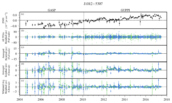
Figure 14: Timing residuals and DM variations for PSR J1012$+$5307. See appendix A text for details. In residual plots, colored points indicate the receiver of each observation: 820 MHz (Green) and 1.4 GHz (Dark blue). (a) Variations in DMX. (b) Residual arrival times for all TOAs. Points are semi-transparent; dark regions arise from the overlap of many points. (c,d) Average residual arrival times shown full scale (panel c) and close-up of low residuals (panel d). (e) Whitened average residual arrival times after removing the red noise model (close-up of low residuals).

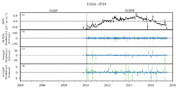
Figure 15: Timing residuals and DM variations for PSR J1024$-$0719. See appendix A text for details. In residual plots, colored points indicate the receiver of each observation: 820 MHz (Green) and 1.4 GHz (Dark blue). (a) Variations in DMX. (b) Residual arrival times for all TOAs. Points are semi-transparent; dark regions arise from the overlap of many points. (c,d) Average residual arrival times shown full scale (panel c) and close-up of low residuals (panel d).

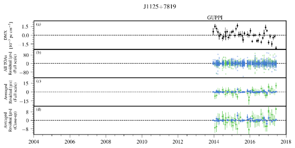
Figure 16: Timing residuals and DM variations for PSR J1125$+$7819. See appendix A text for details. In residual plots, colored points indicate the receiver of each observation: 820 MHz (Green) and 1.4 GHz (Dark blue). (a) Variations in DMX. (b) Residual arrival times for all TOAs. Points are semi-transparent; dark regions arise from the overlap of many points. (c,d) Average residual arrival times shown full scale (panel c) and close-up of low residuals (panel d).

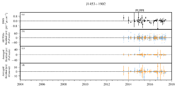
Figure 17: Timing residuals and DM variations for PSR J1453$+$1902. See appendix A text for details. In residual plots, colored points indicate the receiver of each observation: 430 MHz (Orange) and 1.4 GHz (Light blue). (a) Variations in DMX. (b) Residual arrival times for all TOAs. Points are semi-transparent; dark regions arise from the overlap of many points. (c,d) Average residual arrival times shown full scale (panel c) and close-up of low residuals (panel d).

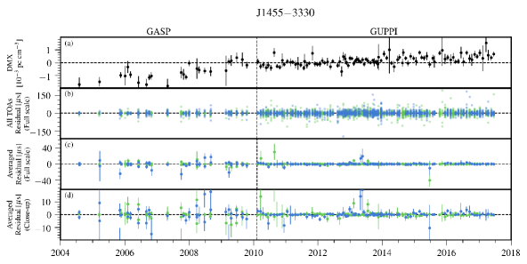
Figure 18: Timing residuals and DM variations for PSR J1455$-$3330. See appendix A text for details. In residual plots, colored points indicate the receiver of each observation: 820 MHz (Green) and 1.4 GHz (Dark blue). (a) Variations in DMX. (b) Residual arrival times for all TOAs. Points are semi-transparent; dark regions arise from the overlap of many points. (c,d) Average residual arrival times shown full scale (panel c) and close-up of low residuals (panel d).

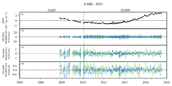
Figure 19: Timing residuals and DM variations for PSR J1600$-$3053. See appendix A text for details. In residual plots, colored points indicate the receiver of each observation: 820 MHz (Green) and 1.4 GHz (Dark blue). (a) Variations in DMX. (b) Residual arrival times for all TOAs. Points are semi-transparent; dark regions arise from the overlap of many points. (c,d) Average residual arrival times shown full scale (panel c) and close-up of low residuals (panel d).

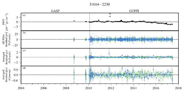
Figure 20: Timing residuals and DM variations for PSR J1614$-$2230. See appendix A text for details. In residual plots, colored points indicate the receiver of each observation: 820 MHz (Green) and 1.4 GHz (Dark blue). (a) Variations in DMX. (b) Residual arrival times for all TOAs. Points are semi-transparent; dark regions arise from the overlap of many points. (c,d) Average residual arrival times shown full scale (panel c) and close-up of low residuals (panel d).

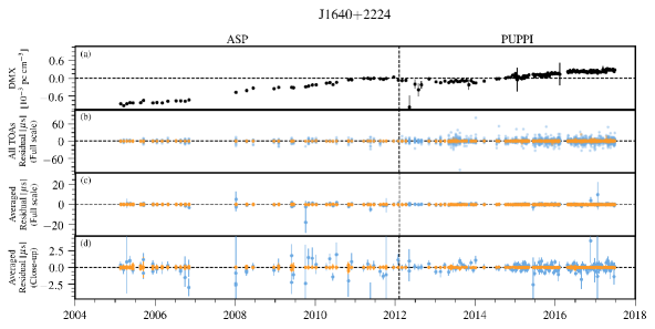
Figure 21: Timing residuals and DM variations for PSR J1640$+$2224. See appendix A text for details. In residual plots, colored points indicate the receiver of each observation: 430 MHz (Orange) and 1.4 GHz (Light blue). (a) Variations in DMX. (b) Residual arrival times for all TOAs. Points are semi-transparent; dark regions arise from the overlap of many points. (c,d) Average residual arrival times shown full scale (panel c) and close-up of low residuals (panel d).

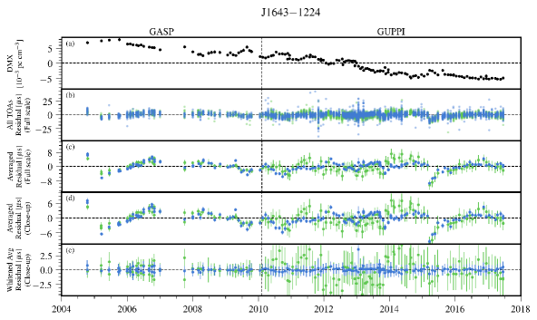
Figure 22: Timing residuals and DM variations for PSR J1643$-$1224. See appendix A text for details. In residual plots, colored points indicate the receiver of each observation: 820 MHz (Green) and 1.4 GHz (Dark blue). (a) Variations in DMX. (b) Residual arrival times for all TOAs. Points are semi-transparent; dark regions arise from the overlap of many points. (c,d) Average residual arrival times shown full scale (panel c) and close-up of low residuals (panel d). (e) Whitened average residual arrival times after removing the red noise model (close-up of low residuals).

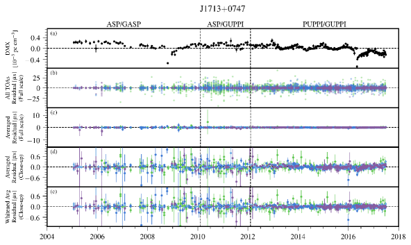
Figure 23: Timing residuals and DM variations for PSR J1713$+$0747. See appendix A text for details. In residual plots, colored points indicate the receiver of each observation: 820 MHz (Green), 1.4 GHz (Dark blue), 1.4 GHz (Light blue), and 2.1 GHz (Purple). (a) Variations in DMX. (b) Residual arrival times for all TOAs. Points are semi-transparent; dark regions arise from the overlap of many points. (c,d) Average residual arrival times shown full scale (panel c) and close-up of low residuals (panel d). (e) Whitened average residual arrival times after removing the red noise model (close-up of low residuals).

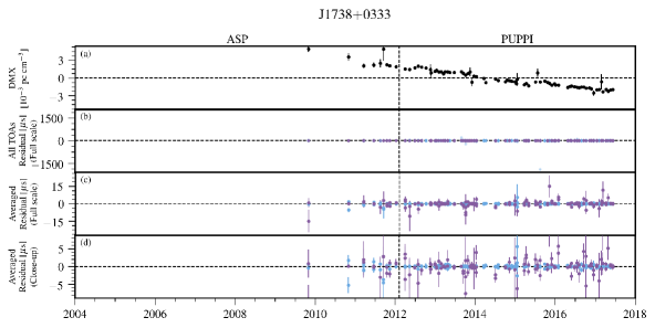
Figure 24: Timing residuals and DM variations for PSR J1738$+$0333. See appendix A text for details. In residual plots, colored points indicate the receiver of each observation: 1.4 GHz (Light blue) and 2.1 GHz (Purple). (a) Variations in DMX. (b) Residual arrival times for all TOAs. Points are semi-transparent; dark regions arise from the overlap of many points. (c,d) Average residual arrival times shown full scale (panel c) and close-up of low residuals (panel d).

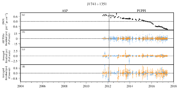
Figure 25: Timing residuals and DM variations for PSR J1741$+$1351. See appendix A text for details. In residual plots, colored points indicate the receiver of each observation: 430 MHz (Orange) and 1.4 GHz (Light blue). (a) Variations in DMX. (b) Residual arrival times for all TOAs. Points are semi-transparent; dark regions arise from the overlap of many points. (c,d) Average residual arrival times shown full scale (panel c) and close-up of low residuals (panel d).

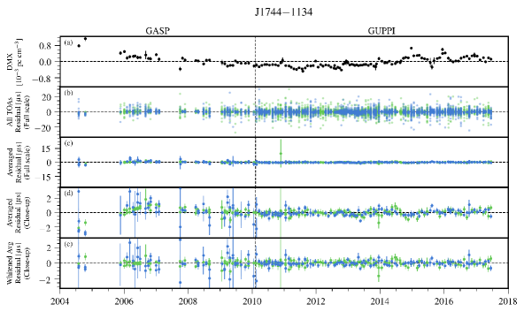
Figure 26: Timing residuals and DM variations for PSR J1744$-$1134. See appendix A text for details. In residual plots, colored points indicate the receiver of each observation: 820 MHz (Green) and 1.4 GHz (Dark blue). (a) Variations in DMX. (b) Residual arrival times for all TOAs. Points are semi-transparent; dark regions arise from the overlap of many points. (c,d) Average residual arrival times shown full scale (panel c) and close-up of low residuals (panel d). (e) Whitened average residual arrival times after removing the red noise model (close-up of low residuals).

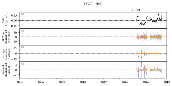
Figure 52: Timing residuals and DM variations for PSR J2322$+$2057. See appendix A text for details. In residual plots, colored points indicate the receiver of each observation: 430 MHz (Orange), 1.4 GHz (Light blue), and 2.1 GHz (Purple). (a) Variations in DMX. (b) Residual arrival times for all TOAs. Points are semi-transparent; dark regions arise from the overlap of many points. (c,d) Average residual arrival times shown full scale (panel c) and close-up of low residuals (panel d).

This appendix includes figures 6–52 showing timing residuals and DM variations for each pulsar in our data set.

DM variations. In panel (a) of each of the appendix figures, we plot the mean-subtracted DM time-series, where each point represents a DM parameter in the DMX model (Section 3.2). The division of each timing baseline into DMX epochs is described in Section 3.2, and the epochs are typically six days in length or less (usually one day for Arecibo observations), except in the earliest data. The mean-subtracted DM values are plotted in part because it allows us to segregate the uncertainty in the average DM, which arises due to covariance with the FD parameters and template pulse profiles, from the uncertainties in the DMX parameters that are shown in the figures.

Timing residuals. As described in Section 2, each observation is comprised of many simultaneously-obtained narrowband TOAs. We plot the residual arrival times (observed minus that predicted from the timing model) for each pulsar in multiple ways described below. In each residual plot, linear and quadratic trends have been removed, as they are completely covariant with the pulsar’s rotation frequency and frequency derivative in the timing model, and hence would be absorbed.

Residuals from every TOA measurement are plotted in panel (b) of each figure. The color of each point encodes the receiver as in Figure 1: 327 MHz (red), 430 MHz (orange), 820 MHz (green), 1400 MHz (lighter blue for AO, darker blue for the GBT), 2100 MHz (purple). The predominant data acquisition backend instrument over any given time period is indicated at the top of each figure, and vertical dashed lines indicate the times at which instruments changed. Averaged residuals of simultaneously measured TOAs are shown in panels (c) and (d); these were computed using the procedure described in Appendix D of NG9. The full vertical range of these residuals is shown in panel (c), while panel (d) shows a close-up of the low residuals. For pulsars with red noise above our defined threshold, red noise Bayes factor $B>100$ (Table 2), panel (e) shows whitened timing residuals, which have the red noise contribution subtracted from the averaged residuals.

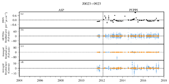
Figure 6: Timing residuals and DM variations for PSR J0023$+$0923. See appendix A text for details. In residual plots, colored points indicate the receiver of each observation: 430 MHz (Orange) and 1.4 GHz (Light blue). (a) Variations in DMX. (b) Residual arrival times for all TOAs. Points are semi-transparent; dark regions arise from the overlap of many points. (c,d) Average residual arrival times shown full scale (panel c) and close-up of low residuals (panel d).

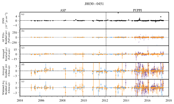
Figure 7: Timing residuals and DM variations for PSR J0030$+$0451. See appendix A text for details. In residual plots, colored points indicate the receiver of each observation: 430 MHz (Orange), 1.4 GHz (Light blue), and 2.1 GHz (Purple). (a) Variations in DMX. (b) Residual arrival times for all TOAs. Points are semi-transparent; dark regions arise from the overlap of many points. (c,d) Average residual arrival times shown full scale (panel c) and close-up of low residuals (panel d). (e) Whitened average residual arrival times after removing the red noise model (close-up of low residuals).

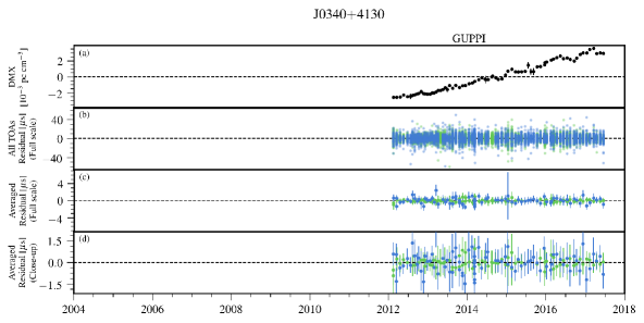
Figure 8: Timing residuals and DM variations for PSR J0340$+$4130. See appendix A text for details. In residual plots, colored points indicate the receiver of each observation: 820 MHz (Green) and 1.4 GHz (Dark blue). (a) Variations in DMX. (b) Residual arrival times for all TOAs. Points are semi-transparent; dark regions arise from the overlap of many points. (c,d) Average residual arrival times shown full scale (panel c) and close-up of low residuals (panel d).

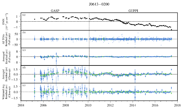
Figure 9: Timing residuals and DM variations for PSR J0613$-$0200. See appendix A text for details. In residual plots, colored points indicate the receiver of each observation: 820 MHz (Green) and 1.4 GHz (Dark blue). (a) Variations in DMX. (b) Residual arrival times for all TOAs. Points are semi-transparent; dark regions arise from the overlap of many points. (c,d) Average residual arrival times shown full scale (panel c) and close-up of low residuals (panel d). (e) Whitened average residual arrival times after removing the red noise model (close-up of low residuals).

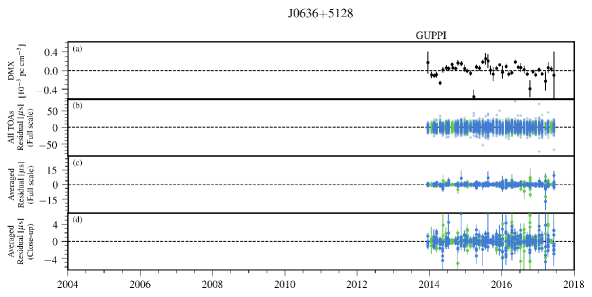
Figure 10: Timing residuals and DM variations for PSR J0636$+$5128. See appendix A text for details. In residual plots, colored points indicate the receiver of each observation: 820 MHz (Green) and 1.4 GHz (Dark blue). (a) Variations in DMX. (b) Residual arrival times for all TOAs. Points are semi-transparent; dark regions arise from the overlap of many points. (c,d) Average residual arrival times shown full scale (panel c) and close-up of low residuals (panel d).

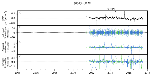
Figure 11: Timing residuals and DM variations for PSR J0645$+$5158. See appendix A text for details. In residual plots, colored points indicate the receiver of each observation: 820 MHz (Green) and 1.4 GHz (Dark blue). (a) Variations in DMX. (b) Residual arrival times for all TOAs. Points are semi-transparent; dark regions arise from the overlap of many points. (c,d) Average residual arrival times shown full scale (panel c) and close-up of low residuals (panel d).

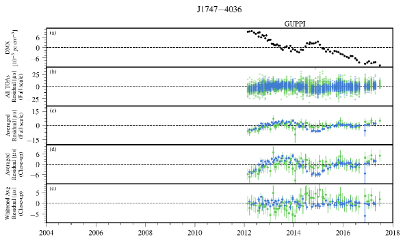
Figure 27: Timing residuals and DM variations for PSR J1747$-$4036. See appendix A text for details. In residual plots, colored points indicate the receiver of each observation: 820 MHz (Green) and 1.4 GHz (Dark blue). (a) Variations in DMX. (b) Residual arrival times for all TOAs. Points are semi-transparent; dark regions arise from the overlap of many points. (c,d) Average residual arrival times shown full scale (panel c) and close-up of low residuals (panel d). (e) Whitened average residual arrival times after removing the red noise model (close-up of low residuals).

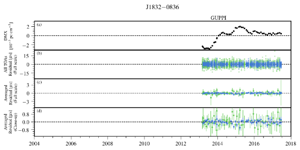
Figure 28: Timing residuals and DM variations for PSR J1832$-$0836. See appendix A text for details. In residual plots, colored points indicate the receiver of each observation: 820 MHz (Green) and 1.4 GHz (Dark blue). (a) Variations in DMX. (b) Residual arrival times for all TOAs. Points are semi-transparent; dark regions arise from the overlap of many points. (c,d) Average residual arrival times shown full scale (panel c) and close-up of low residuals (panel d).

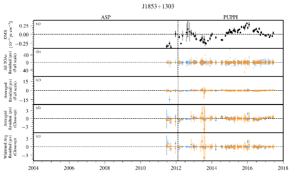
Figure 29: Timing residuals and DM variations for PSR J1853$+$1303. See appendix A text for details. In residual plots, colored points indicate the receiver of each observation: 430 MHz (Orange) and 1.4 GHz (Light blue). (a) Variations in DMX. (b) Residual arrival times for all TOAs. Points are semi-transparent; dark regions arise from the overlap of many points. (c,d) Average residual arrival times shown full scale (panel c) and close-up of low residuals (panel d). (e) Whitened average residual arrival times after removing the red noise model (close-up of low residuals).

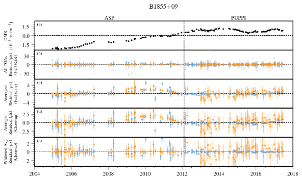
Figure 30: Timing residuals and DM variations for PSR B1855$+$09. See appendix A text for details. In residual plots, colored points indicate the receiver of each observation: 430 MHz (Orange) and 1.4 GHz (Light blue). (a) Variations in DMX. (b) Residual arrival times for all TOAs. Points are semi-transparent; dark regions arise from the overlap of many points. (c,d) Average residual arrival times shown full scale (panel c) and close-up of low residuals (panel d). (e) Whitened average residual arrival times after removing the red noise model (close-up of low residuals).

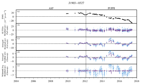
Figure 31: Timing residuals and DM variations for PSR J1903$+$0327. See appendix A text for details. In residual plots, colored points indicate the receiver of each observation: 1.4 GHz (Light blue) and 2.1 GHz (Purple). (a) Variations in DMX. (b) Residual arrival times for all TOAs. Points are semi-transparent; dark regions arise from the overlap of many points. (c,d) Average residual arrival times shown full scale (panel c) and close-up of low residuals (panel d). (e) Whitened average residual arrival times after removing the red noise model (close-up of low residuals).

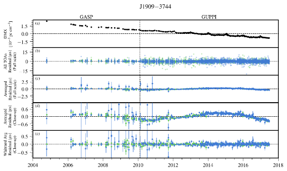
Figure 32: Timing residuals and DM variations for PSR J1909$-$3744. See appendix A text for details. In residual plots, colored points indicate the receiver of each observation: 820 MHz (Green) and 1.4 GHz (Dark blue). (a) Variations in DMX. (b) Residual arrival times for all TOAs. Points are semi-transparent; dark regions arise from the overlap of many points. (c,d) Average residual arrival times shown full scale (panel c) and close-up of low residuals (panel d). (e) Whitened average residual arrival times after removing the red noise model (close-up of low residuals).

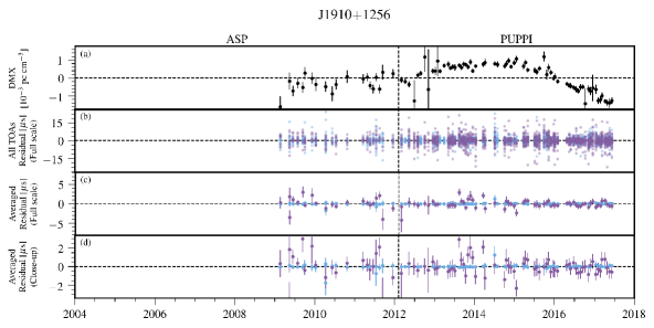
Figure 33: Timing residuals and DM variations for PSR J1910$+$1256. See appendix A text for details. In residual plots, colored points indicate the receiver of each observation: 1.4 GHz (Light blue) and 2.1 GHz (Purple). (a) Variations in DMX. (b) Residual arrival times for all TOAs. Points are semi-transparent; dark regions arise from the overlap of many points. (c,d) Average residual arrival times shown full scale (panel c) and close-up of low residuals (panel d).

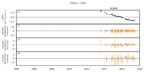
Figure 34: Timing residuals and DM variations for PSR J1911$+$1347. See appendix A text for details. In residual plots, colored points indicate the receiver of each observation: 430 MHz (Orange) and 1.4 GHz (Light blue). (a) Variations in DMX. (b) Residual arrival times for all TOAs. Points are semi-transparent; dark regions arise from the overlap of many points. (c,d) Average residual arrival times shown full scale (panel c) and close-up of low residuals (panel d).

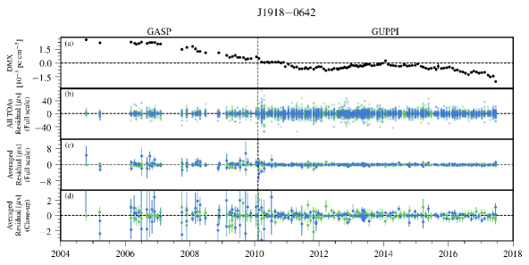
Figure 35: Timing residuals and DM variations for PSR J1918$-$0642. See appendix A text for details. In residual plots, colored points indicate the receiver of each observation: 820 MHz (Green) and 1.4 GHz (Dark blue). (a) Variations in DMX. (b) Residual arrival times for all TOAs. Points are semi-transparent; dark regions arise from the overlap of many points. (c,d) Average residual arrival times shown full scale (panel c) and close-up of low residuals (panel d).

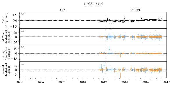
Figure 36: Timing residuals and DM variations for PSR J1923$+$2515. See appendix A text for details. In residual plots, colored points indicate the receiver of each observation: 430 MHz (Orange) and 1.4 GHz (Light blue). (a) Variations in DMX. (b) Residual arrival times for all TOAs. Points are semi-transparent; dark regions arise from the overlap of many points. (c,d) Average residual arrival times shown full scale (panel c) and close-up of low residuals (panel d).

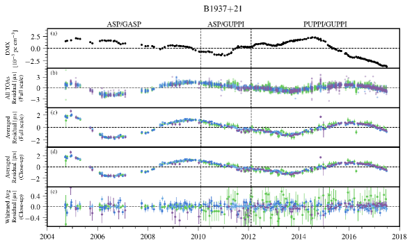
Figure 37: Timing residuals and DM variations for PSR B1937$+$21. See appendix A text for details. In residual plots, colored points indicate the receiver of each observation: 820 MHz (Green), 1.4 GHz (Dark blue), 1.4 GHz (Light blue), and 2.1 GHz (Purple). (a) Variations in DMX. (b) Residual arrival times for all TOAs. Points are semi-transparent; dark regions arise from the overlap of many points. (c,d) Average residual arrival times shown full scale (panel c) and close-up of low residuals (panel d). (e) Whitened average residual arrival times after removing the red noise model (close-up of low residuals).

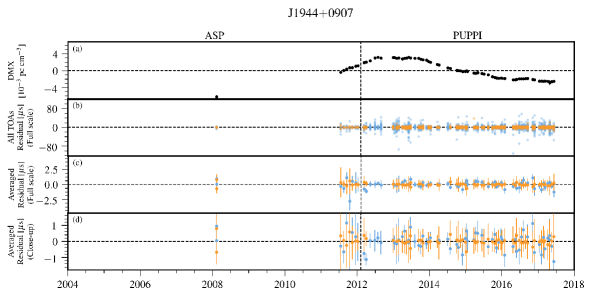
Figure 38: Timing residuals and DM variations for PSR J1944$+$0907. See appendix A text for details. In residual plots, colored points indicate the receiver of each observation: 430 MHz (Orange) and 1.4 GHz (Light blue). (a) Variations in DMX. (b) Residual arrival times for all TOAs. Points are semi-transparent; dark regions arise from the overlap of many points. (c,d) Average residual arrival times shown full scale (panel c) and close-up of low residuals (panel d).

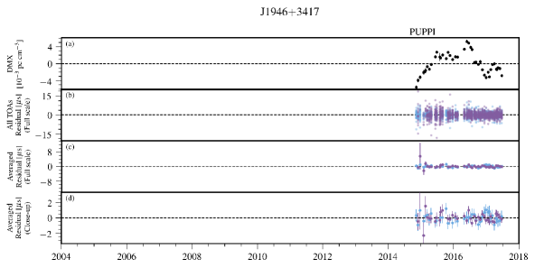
Figure 39: Timing residuals and DM variations for PSR J1946$+$3417. See appendix A text for details. In residual plots, colored points indicate the receiver of each observation: 1.4 GHz (Light blue) and 2.1 GHz (Purple). (a) Variations in DMX. (b) Residual arrival times for all TOAs. Points are semi-transparent; dark regions arise from the overlap of many points. (c,d) Average residual arrival times shown full scale (panel c) and close-up of low residuals (panel d).

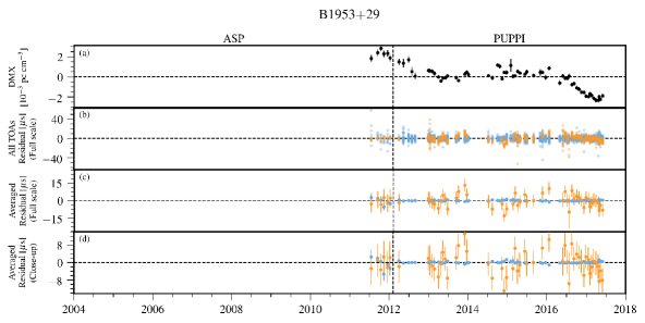
Figure 40: Timing residuals and DM variations for PSR B1953$+$29. See appendix A text for details. In residual plots, colored points indicate the receiver of each observation: 430 MHz (Orange) and 1.4 GHz (Light blue). (a) Variations in DMX. (b) Residual arrival times for all TOAs. Points are semi-transparent; dark regions arise from the overlap of many points. (c,d) Average residual arrival times shown full scale (panel c) and close-up of low residuals (panel d).

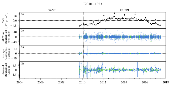
Figure 41: Timing residuals and DM variations for PSR J2010$-$1323. See appendix A text for details. In residual plots, colored points indicate the receiver of each observation: 820 MHz (Green) and 1.4 GHz (Dark blue). (a) Variations in DMX. (b) Residual arrival times for all TOAs. Points are semi-transparent; dark regions arise from the overlap of many points. (c,d) Average residual arrival times shown full scale (panel c) and close-up of low residuals (panel d).

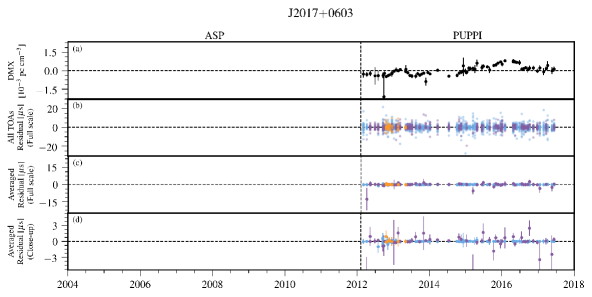
Figure 42: Timing residuals and DM variations for PSR J2017$+$0603. See appendix A text for details. In residual plots, colored points indicate the receiver of each observation: 430 MHz (Orange), 1.4 GHz (Light blue), and 2.1 GHz (Purple). (a) Variations in DMX. (b) Residual arrival times for all TOAs. Points are semi-transparent; dark regions arise from the overlap of many points. (c,d) Average residual arrival times shown full scale (panel c) and close-up of low residuals (panel d).

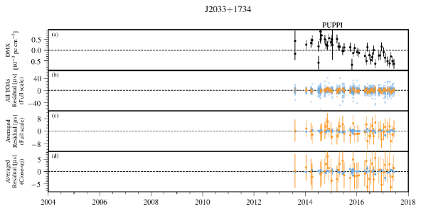
Figure 43: Timing residuals and DM variations for PSR J2033$+$1734. See appendix A text for details. In residual plots, colored points indicate the receiver of each observation: 430 MHz (Orange) and 1.4 GHz (Light blue). (a) Variations in DMX. (b) Residual arrival times for all TOAs. Points are semi-transparent; dark regions arise from the overlap of many points. (c,d) Average residual arrival times shown full scale (panel c) and close-up of low residuals (panel d).

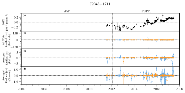
Figure 44: Timing residuals and DM variations for PSR J2043$+$1711. See appendix A text for details. In residual plots, colored points indicate the receiver of each observation: 430 MHz (Orange) and 1.4 GHz (Light blue). (a) Variations in DMX. (b) Residual arrival times for all TOAs. Points are semi-transparent; dark regions arise from the overlap of many points. (c,d) Average residual arrival times shown full scale (panel c) and close-up of low residuals (panel d).

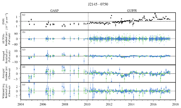
Figure 45: Timing residuals and DM variations for PSR J2145$-$0750. See appendix A text for details. In residual plots, colored points indicate the receiver of each observation: 820 MHz (Green) and 1.4 GHz (Dark blue). (a) Variations in DMX. (b) Residual arrival times for all TOAs. Points are semi-transparent; dark regions arise from the overlap of many points. (c,d) Average residual arrival times shown full scale (panel c) and close-up of low residuals (panel d). (e) Whitened average residual arrival times after removing the red noise model (close-up of low residuals).

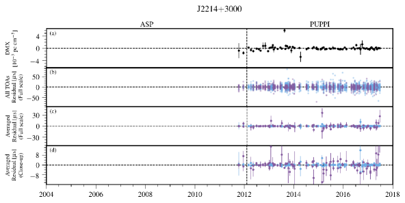
Figure 46: Timing residuals and DM variations for PSR J2214$+$3000. See appendix A text for details. In residual plots, colored points indicate the receiver of each observation: 1.4 GHz (Light blue) and 2.1 GHz (Purple). (a) Variations in DMX. (b) Residual arrival times for all TOAs. Points are semi-transparent; dark regions arise from the overlap of many points. (c,d) Average residual arrival times shown full scale (panel c) and close-up of low residuals (panel d).

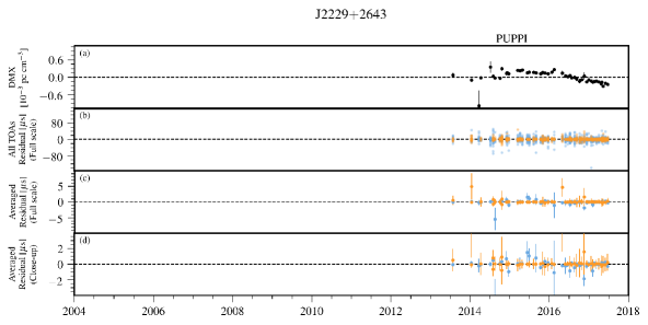
Figure 47: Timing residuals and DM variations for PSR J2229$+$2643. See appendix A text for details. In residual plots, colored points indicate the receiver of each observation: 430 MHz (Orange) and 1.4 GHz (Light blue). (a) Variations in DMX. (b) Residual arrival times for all TOAs. Points are semi-transparent; dark regions arise from the overlap of many points. (c,d) Average residual arrival times shown full scale (panel c) and close-up of low residuals (panel d).

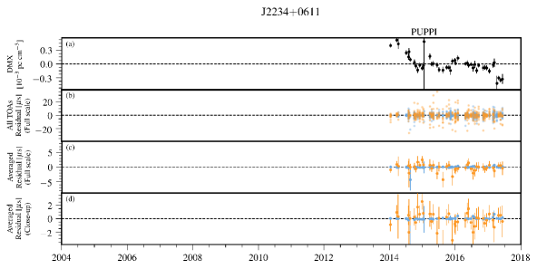
Figure 48: Timing residuals and DM variations for PSR J2234$+$0611. See appendix A text for details. In residual plots, colored points indicate the receiver of each observation: 430 MHz (Orange) and 1.4 GHz (Light blue). (a) Variations in DMX. (b) Residual arrival times for all TOAs. Points are semi-transparent; dark regions arise from the overlap of many points. (c,d) Average residual arrival times shown full scale (panel c) and close-up of low residuals (panel d).

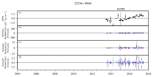
Figure 49: Timing residuals and DM variations for PSR J2234$+$0944. See appendix A text for details. In residual plots, colored points indicate the receiver of each observation: 1.4 GHz (Light blue) and 2.1 GHz (Purple). (a) Variations in DMX. (b) Residual arrival times for all TOAs. Points are semi-transparent; dark regions arise from the overlap of many points. (c,d) Average residual arrival times shown full scale (panel c) and close-up of low residuals (panel d).

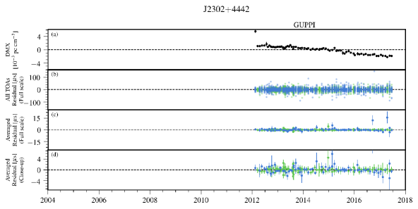
Figure 50: Timing residuals and DM variations for PSR J2302$+$4442. See appendix A text for details. In residual plots, colored points indicate the receiver of each observation: 820 MHz (Green) and 1.4 GHz (Dark blue). (a) Variations in DMX. (b) Residual arrival times for all TOAs. Points are semi-transparent; dark regions arise from the overlap of many points. (c,d) Average residual arrival times shown full scale (panel c) and close-up of low residuals (panel d).

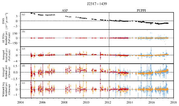
Figure 51: Timing residuals and DM variations for PSR J2317$+$1439. See appendix A text for details. In residual plots, colored points indicate the receiver of each observation: 327 MHz (Red), 430 MHz (Orange), and 1.4 GHz (Light blue). (a) Variations in DMX. (b) Residual arrival times for all TOAs. Points are semi-transparent; dark regions arise from the overlap of many points. (c,d) Average residual arrival times shown full scale (panel c) and close-up of low residuals (panel d). (e) Whitened average residual arrival times after removing the red noise model (close-up of low residuals).

References

- Aggarwal et al. (2019) Aggarwal, K., Arzoumanian, Z., Baker, P. T., et al. 2019, ApJ, 880, 116, doi: 10.3847/1538-4357/ab2236
- Aggarwal et al. (2020) —. 2020, ApJ, 889, 38, doi: 10.3847/1538-4357/ab6083
- Alam et al. (2020) Alam, M. F., Arzoumanian, Z., Baker, P. T., et al. 2020, The Astrophysical Journal Supplement Series, 252, 4, doi: 10.3847/1538-4365/abc6a1
- Arzoumanian et al. (2014) Arzoumanian, Z., Brazier, A., Burke-Spolaor, S., et al. 2014, ApJ, 794, 141, doi: 10.1088/0004-637X/794/2/141
- Arzoumanian et al. (2015) —. 2015, ApJ, 813, 65, doi: 10.1088/0004-637X/813/1/65
- Arzoumanian et al. (2018a) —. 2018a, ApJS, 235, 37, doi: 10.3847/1538-4365/aab5b0
- Arzoumanian et al. (2018b) Arzoumanian, Z., Baker, P. T., Brazier, A., et al. 2018b, ApJ, 859, 47, doi: 10.3847/1538-4357/aabd3b
- Arzoumanian et al. (2020) Arzoumanian, Z., Baker, P. T., Blumer, H., et al. 2020, arXiv e-prints, arXiv:2009.04496. https://arxiv.org/abs/2009.04496
- Bak Nielsen et al. (2020) Bak Nielsen, A.-S., Janssen, G. H., Shaifullah, G., et al. 2020, MNRAS, 494, 2591, doi: 10.1093/mnras/staa874
- Barr et al. (2017) Barr, E. D., Freire, P. C. C., Kramer, M., et al. 2017, MNRAS, 465, 1711, doi: 10.1093/mnras/stw2947
- Burke-Spolaor et al. (2019) Burke-Spolaor, S., Taylor, S. R., Charisi, M., et al. 2019, A&A Rev., 27, 5, doi: 10.1007/s00159-019-0115-7
- Cromartie et al. (2020) Cromartie, H. T., Fonseca, E., Ransom, S. M., et al. 2020, Nature Astronomy, 4, 72, doi: 10.1038/s41550-019-0880-2
- Damour & Deruelle (1985) Damour, T., & Deruelle, N. 1985, Ann. Inst. Henri Poincaré Phys. Théor., Vol. 43, No. 1, p. 107 - 132, 43, 107
- Damour & Deruelle (1986) —. 1986, Ann. Inst. Henri Poincaré Phys. Théor., Vol. 44, No. 3, p. 263 - 292, 44, 263
- Damour & Taylor (1992) Damour, T., & Taylor, J. H. 1992, Phys. Rev. D, 45, 1840, doi: 10.1103/PhysRevD.45.1840
- Deller et al. (2016) Deller, A. T., Vigeland, S. J., Kaplan, D. L., et al. 2016, ApJ, 828, 8, doi: 10.3847/0004-637X/828/1/8
- Deller et al. (2019) Deller, A. T., Goss, W. M., Brisken, W. F., et al. 2019, ApJ, 875, 100, doi: 10.3847/1538-4357/ab11c7
- Demorest (2007) Demorest, P. B. 2007, PhD thesis, University of California, Berkeley
- Demorest (2018) —. 2018, nanopipe: Calibration and data reduction pipeline for pulsar timing, Astrophysics Source Code Library. http://ascl.net/1803.004, git commit d8ec4e4 on 2018-09-17
- Demorest et al. (2013) Demorest, P. B., Ferdman, R. D., Gonzalez, M. E., et al. 2013, ApJ, 762, 94, doi: 10.1088/0004-637X/762/2/94
- Deneva et al. (2019) Deneva, J. S., Ray, P. S., Lommen, A., et al. 2019, ApJ, 874, 160, doi: 10.3847/1538-4357/ab0966
- Desvignes et al. (2016) Desvignes, G., Caballero, R. N., Lentati, L., et al. 2016, MNRAS, 458, 3341, doi: 10.1093/mnras/stw483
- Dickey (1971) Dickey, J. M. 1971, Ann. Math. Statist., 42, 204, doi: 10.1214/aoms/1177693507
- Ding et al. (2020) Ding, H., Deller, A. T., Freire, P., et al. 2020, ApJ, 896, 85, doi: 10.3847/1538-4357/ab8f27
- DuPlain et al. (2008) DuPlain, R., Ransom, S., Demorest, P., et al. 2008, in Proc. SPIE, Vol. 7019, Advanced Software and Control for Astronomy II, 70191D, doi: 10.1117/12.790003
- Ellis & van Haasteren (2017) Ellis, J., & van Haasteren, R. 2017, jellis18/PTMCMCSampler: Official Release, doi: 10.5281/zenodo.1037579, version 1.0.0
- Ellis et al. (2019) Ellis, J. A., Vallisneri, M., Taylor, S. R., & Baker, P. T. 2019, ENTERPRISE: Enhanced Numerical Toolbox Enabling a Robust PulsaR Inference SuitE. http://ascl.net/1912.015, version 2.0
- Fonseca et al. (2016) Fonseca, E., Pennucci, T. T., Ellis, J. A., et al. 2016, ApJ, 832, 167, doi: 10.3847/0004-637X/832/2/167
- Ford et al. (2010) Ford, J. M., Demorest, P., & Ransom, S. 2010, in Proc. SPIE, Vol. 7740, Software and Cyberinfrastructure for Astronomy, 77400A, doi: 10.1117/12.857666
- Frail et al. (2016) Frail, D. A., Jagannathan, P., Mooley, K. P., & Intema, H. T. 2016, ApJ, 829, 119, doi: 10.3847/0004-637X/829/2/119
- Freire & Wex (2010) Freire, P. C. C., & Wex, N. 2010, MNRAS, 409, 199, doi: 10.1111/j.1365-2966.2010.17319.x
- Gonzalez et al. (2011) Gonzalez, M. E., Stairs, I. H., Ferdman, R. D., et al. 2011, ApJ, 743, 102, doi: 10.1088/0004-637X/743/2/102
- Hazboun et al. (2020) Hazboun, J. S., Simon, J., Taylor, S. R., et al. 2020, ApJ, 890, 108, doi: 10.3847/1538-4357/ab68db
- Hobbs & Edwards (2012) Hobbs, G., & Edwards, R. 2012, Tempo2: Pulsar Timing Package. http://ascl.net/1210.015, version 2019.01.1
- Hobbs et al. (2010) Hobbs, G., Archibald, A., Arzoumanian, Z., et al. 2010, Classical and Quantum Gravity, 27, 084013, doi: 10.1088/0264-9381/27/8/084013
- Hotan et al. (2004) Hotan, A. W., van Straten, W., & Manchester, R. N. 2004, Proc. Astron. Soc. Aust., 21, 302, doi: 10.1071/AS04022
- Hunter (2007) Hunter, J. D. 2007, Computing In Science & Engineering, 9, 90, doi: 10.1109/MCSE.2007.55
- Jones et al. (2017) Jones, M. L., McLaughlin, M. A., Lam, M. T., et al. 2017, ApJ, 841, 125, doi: 10.3847/1538-4357/aa73df
- Kerr et al. (2020) Kerr, M., Reardon, D. J., Hobbs, G., et al. 2020, PASA, 37, e020, doi: 10.1017/pasa.2020.11
- Kopeikin (1995) Kopeikin, S. M. 1995, ApJ, 439, L5, doi: 10.1086/187731
- Kopeikin (1996) —. 1996, ApJ, 467, L93, doi: 10.1086/310201
- Kramer et al. (1998) Kramer, M., Xilouris, K. M., Lorimer, D. R., et al. 1998, ApJ, 501, 270, doi: 10.1086/305790
- Kurosawa et al. (2001) Kurosawa, N., Kobayashi, H., Maruyama, K., Sugawara, H., & Kobayashi, K. 2001, IEEE Transactions on Circuits and Systems I: Fundamental Theory and Applications, 48, 261, doi: 10.1109/81.915383
- Lam (2017) Lam, M. T. 2017, PyPulse: PSRFITS handler. http://ascl.net/1706.011, git commit 4c0f24 on 06-08-2019
- Lam et al. (2018a) Lam, M. T., McLaughlin, M. A., Cordes, J. M., Chatterjee, S., & Lazio, T. J. W. 2018a, ApJ, 861, 12, doi: 10.3847/1538-4357/aac48d
- Lam et al. (2016) Lam, M. T., Cordes, J. M., Chatterjee, S., et al. 2016, ApJ, 819, 155, doi: 10.3847/0004-637X/819/2/155
- Lam et al. (2018b) Lam, M. T., Ellis, J. A., Grillo, G., et al. 2018b, ApJ, 861, 132, doi: 10.3847/1538-4357/aac770
- Lam et al. (2019) Lam, M. T., McLaughlin, M. A., Arzoumanian, Z., et al. 2019, ApJ, 872, 193, doi: 10.3847/1538-4357/ab01cd
- Lange et al. (2001) Lange, C., Camilo, F., Wex, N., et al. 2001, MNRAS, 326, 274, doi: 10.1046/j.1365-8711.2001.04606.x
- Lattimer (2019) Lattimer, J. M. 2019, Universe, 5, 159, doi: 10.3390/universe5070159
- Liu et al. (2014) Liu, K., Desvignes, G., Cognard, I., et al. 2014, MNRAS, 443, 3752, doi: 10.1093/mnras/stu1420
- Lorimer et al. (2006) Lorimer, D. R., Faulkner, A. J., Lyne, A. G., et al. 2006, MNRAS, 372, 777, doi: 10.1111/j.1365-2966.2006.10887.x
- Luo et al. (2019) Luo, J., Ransom, S., Demorest, P., et al. 2019, PINT: High-precision pulsar timing analysis package. http://ascl.net/1902.007, version 0.5.7
- Luo et al. (2020) —. 2020, arXiv e-prints, arXiv:2012.00074. https://arxiv.org/abs/2012.00074
- Madison et al. (2019) Madison, D. R., Cordes, J. M., Arzoumanian, Z., et al. 2019, ApJ, 872, 150, doi: 10.3847/1538-4357/ab01fd
- Manchester et al. (2005) Manchester, R. N., Hobbs, G. B., Teoh, A., & Hobbs, M. 2005, AJ, 129, 1993, doi: 10.1086/428488
- Matthews et al. (2016) Matthews, A. M., Nice, D. J., Fonseca, E., et al. 2016, ApJ, 818, 92, doi: 10.3847/0004-637X/818/1/92
- Nice et al. (2015) Nice, D., Demorest, P., Stairs, I., et al. 2015, Tempo: Pulsar timing data analysis. http://ascl.net/1509.002, version 13.000, git commit 3452a0c on 2019-01-17
- Nice & Taylor (1995) Nice, D. J., & Taylor, J. H. 1995, ApJ, 441, 429, doi: 10.1086/175367
- Osłowski et al. (2011) Osłowski, S., van Straten, W., Hobbs, G. B., Bailes, M., & Demorest, P. 2011, MNRAS, 418, 1258, doi: 10.1111/j.1365-2966.2011.19578.x
- Pennucci (2019) Pennucci, T. T. 2019, ApJ, 871, 34, doi: 10.3847/1538-4357/aaf6ef
- Pennucci et al. (2014) Pennucci, T. T., Demorest, P. B., & Ransom, S. M. 2014, ApJ, 790, 93, doi: 10.1088/0004-637X/790/2/93
- Perera et al. (2019) Perera, B. B. P., DeCesar, M. E., Demorest, P. B., et al. 2019, MNRAS, 490, 4666, doi: 10.1093/mnras/stz2857
- Perrodin & Sesana (2018) Perrodin, D., & Sesana, A. 2018, in Astrophysics and Space Science Library, Vol. 457, Astrophysics and Space Science Library, ed. L. Rezzolla, P. Pizzochero, D. I. Jones, N. Rea, & I. Vidaña, 95, doi: 10.1007/978-3-319-97616-7_3
- Ransom et al. (2019) Ransom, S., Brazier, A., Chatterjee, S., et al. 2019, in BAAS, Vol. 51, 195. https://arxiv.org/abs/1908.05356
- Ransom et al. (2011) Ransom, S. M., Ray, P. S., Camilo, F., et al. 2011, ApJ, 727, L16, doi: 10.1088/2041-8205/727/1/L16
- Reardon et al. (2016) Reardon, D. J., Hobbs, G., Coles, W., et al. 2016, MNRAS, 455, 1751, doi: 10.1093/mnras/stv2395
- Renevey (2019) Renevey, C. 2019, arXiv e-prints, arXiv:1905.13720. https://arxiv.org/abs/1905.13720
- Shaifullah (2017) Shaifullah, G. 2017, PhD thesis, Universität Bielefeld
- Shannon et al. (2014) Shannon, R. M., Osłowski, S., Dai, S., et al. 2014, MNRAS, 443, 1463, doi: 10.1093/mnras/stu1213
- Siemens et al. (2013) Siemens, X., Ellis, J., Jenet, F., & Romano, J. D. 2013, Classical and Quantum Gravity, 30, 224015, doi: 10.1088/0264-9381/30/22/224015
- Simon et al. (2020) Simon, J. et al. 2020, in preparation
- Splaver et al. (2005) Splaver, E. M., Nice, D. J., Stairs, I. H., Lommen, A. N., & Backer, D. C. 2005, ApJ, 620, 405, doi: 10.1086/426804
- Stovall et al. (2014) Stovall, K., Lynch, R. S., Ransom, S. M., et al. 2014, ApJ, 791, 67, doi: 10.1088/0004-637X/791/1/67
- Stovall et al. (2019) Stovall, K., Freire, P. C. C., Antoniadis, J., et al. 2019, ApJ, 870, 74, doi: 10.3847/1538-4357/aaf37d
- Taylor et al. (2016) Taylor, S. R., Vallisneri, M., Ellis, J. A., et al. 2016, ApJ, 819, L6, doi: 10.3847/2041-8205/819/1/L6
- Vallisneri (2020) Vallisneri, M. 2020, libstempo: Python wrapper for Tempo2. http://ascl.net/2002.017
- Vallisneri & van Haasteren (2017) Vallisneri, M., & van Haasteren, R. 2017, MNRAS, 466, 4954, doi: 10.1093/mnras/stx069
- van Haasteren (2016) van Haasteren, R. 2016, Piccard: Pulsar timing data analysis package. http://ascl.net/1610.001, version 2.3.4
- van Straten et al. (2011) van Straten, W., Demorest, P., Khoo, J., et al. 2011, PSRCHIVE: Development Library for the Analysis of Pulsar Astronomical Data. http://ascl.net/1105.014, version v0.9-sp
- Verbiest et al. (2012) Verbiest, J. P. W., Weisberg, J. M., Chael, A. A., Lee, K. J., & Lorimer, D. R. 2012, ApJ, 755, 39, doi: 10.1088/0004-637X/755/1/39
- Verbiest et al. (2009) Verbiest, J. P. W., Bailes, M., Coles, W. A., et al. 2009, MNRAS, 400, 951, doi: 10.1111/j.1365-2966.2009.15508.x
- Wang et al. (2017) Wang, J. B., Coles, W. A., Hobbs, G., et al. 2017, MNRAS, 469, 425, doi: 10.1093/mnras/stx837
- Weisberg & Huang (2016) Weisberg, J. M., & Huang, Y. 2016, ApJ, 829, 55, doi: 10.3847/0004-637X/829/1/55