The effect of Target Normalization and Momentum on Dying ReLU

Abstract

Optimizing parameters with momentum, normalizing data values, and using rectified linear units (ReLUs) are popular choices in neural network (NN) regression. Although ReLUs are popular, they can collapse to a constant function and “die”, effectively removing their contribution from the model. While some mitigations are known, the underlying reasons of ReLUs dying during optimization are currently poorly understood. In this paper, we consider the effects of target normalization and momentum on dying ReLUs. We find empirically that unit variance targets are well motivated and that ReLUs die more easily, when target variance approaches zero. To further investigate this matter, we analyze a discrete-time linear autonomous system, and show theoretically how this relates to a model with a single ReLU and how common properties can result in dying ReLU. We also analyze the gradients of a single-ReLU model to identify saddle points and regions corresponding to dying ReLU and how parameters evolve into these regions when momentum is used. Finally, we show empirically that this problem persist, and is aggravated, for deeper models including residual networks.

1 Introduction

Gradient-based optimization enables learning of powerful deep NN models [1, 2]. However, most learning algorithms remain sensitive to learning rate, scale of data values, and the choice of activation function—making deep NN models hard to train [3, 4]. Stochastic gradient descent with momentum [5, 6], normalizing data values to have zero mean and unit variance [7], and employing rectified linear units (ReLUs) in NNs [8, 9, 10] have emerged as an empirically motivated and popular practice. In this paper, we analyze a specific failure case of this practice, referred to as “dying” ReLU.

The ReLU activation function, $y=\max\{x,0\}$ is a popular choice of activation function and has been shown to have superior training performance in various domains [11, 12]. ReLUs can sometimes be collapse to a constant (zero) function for a given set of inputs. Such a ReLU is considered “dead” and does not contribute to a learned model. ReLUs can be initialized dead [13] or die during optimization, the latter being a major obstacle in training deep NNs [14, 15]. Once dead, gradients are zero making recovery possible only if inputs change distribution. Over time, large parts of a NN can end up dead which reduces model capacity.

Mitigations to dying ReLU include modifying the ReLU to also activate for negative inputs [16, 17, 18], training procedures with normalization steps [19, 20], and initialization methods [13]. While these approaches have some success in practice, the underlying cause for ReLUs dying during optimization is, to our knowledge, still not understood.

Figure 1: The performance of models, in terms of fit to the training data, degrades as the variance ($\gamma$) of target values deviate from $1$, or the mean ($\delta$) deviates from $0$. Here shown in terms of mean-squared error (MSE) on four different datasets [21]. Furthermore, decreasing $\gamma$ leads to more dying ReLUs only with the use of momentum optimization [6]. Details of this experiment can be found in Appendix A.

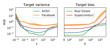
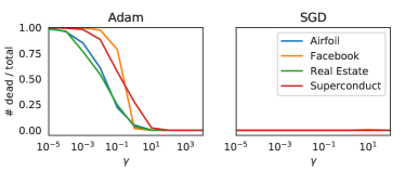
In this paper, we analyze the observation illustrated in Figure 1 that regression performance degrades with smaller target variances, and along with momentum optimization leads to dead ReLU. Although target normalization is a common pre-processing step, we believe a scientific understanding of why it is important is missing, especially with the connection to momentum optimization. For our theoretical results, we first show that an affine approximator trained with gradient descent and momentum corresponds to a discrete-time linear autonomous system. Introducing momentum into this system results in complex eigenvalues and parameters that oscillate. We further show that a single-ReLU model has two cones in parameter space; one for which the properties of the linear system is shared, and one that corresponds to dead ReLU.

We derive analytic gradients for the single-ReLU model to further gain insight and to identify critical points (i.e. global optima and saddle points) in parameter space. By inspection of numerical examples, we also identify regions where ReLUs tend to converge to the global optimum (without dying) and how these regions change with momentum. Lastly, we show empirically that the problem of dying ReLU is aggravated in deeper models, including residual neural networks.

2 Related work

In a recent paper [13], the authors identify dying ReLUs as a cause of vanishing gradients. This is a fundamental problem in NNs [22, 23]. In general, this can be caused by ReLUs being initialized dead or dying during optimization. Theoretical results about initialization and dead ReLU NNs are presented by Lu et al. [13]. Growing NN depth towards infinity and initializing parameters from symmetric distributions both lead to dead models. However, asymmetric initialization can effectively prevent this outcome. Empirical results about ReLUs dying during optimization are presented by Wu et al. [24]. Similar to us, they observe a relationship between dying ReLUs and the scale of target values. In contrast to us, they do not investigate the underlying cause.

Normalization of layer input values.

The effects of input value distribution has been studied for a long time, e.g. [25]. Inputs with zero mean have been shown to result in gradients that more closely resemble the natural gradient, which speeds up training [26]. In fact, a range of strategies to normalize layer input data exists [20, 19, 27] along with theoretical analysis of the problem [28]. Another studied area for maintaining statistics throughout the NN is initialization of the parameters [29, 18, 13]. However, subsequent optimization steps may change the parameters such that the desired input mean and variance no longer is fulfilled.

Normalization of target values.

When the training data are available before optimization, target normalization is trivially executed. More challenging is the case where training data are accessed incrementally, e.g. as in reinforcement learning or for very large training data. Here, normalization and scaling of target values are important for the learning outcome [30, 31, 24]. For on-line regression and reinforcement learning, adaptive target normalization improves results and removes the need of gradient clipping [30]. In reinforcement learning, scaling rewards by a positive constant is crucial for learning performance, and is often equivalent to the scaling of target values [31]. Small reward scales have been seen to increase the risk of dying ReLUs [24]. All of these works motivate the use of target normalization empirically and a theoretical understanding is still lacking. In this paper, we provide more insight into the relationship between dying ReLUs and target normalization.

3 Preliminaries

We consider regression of a target function $y\colon\mathbb{R}^{L}\to\mathbb{R}$ from training data $\mathcal{D}=\{(\mathbf{x}^{(i)},y_{*}^{(i)})\}_{i}$ consisting of pairs of inputs $\mathbf{x}^{(i)}\in\mathbb{R}^{L}$ and target values $y_{*}^{(i)}=y(\mathbf{x}^{(i)})\in\mathbb{R}$. We analyze different regression models $\hat{y}$, such as an affine transformation in Sec. 4 and a ReLU-activated model in Sec. 5, which are both parameterized by a vector $\boldsymbol{\theta}$. Below, we provide definitions, notations, and equalities needed for our analysis.

Target normalization.

Before regression, we transform target values $y_{*}^{(i)}$ according to

$$y^{(i)}=\gamma\frac{y_{*}^{(i)}-\hat{\mu}}{\hat{\sigma}}+\delta,$$ (1)

where $\hat{\mu}$ and $\hat{\sigma}$ are mean and standard deviation of the target values from the training data. When the parameters of the transform are set to scale $\gamma=1$ and bias $\delta=0$, new target values $y^{(i)}$ correspond to $z$-normalization [32] with zero mean and unit variance. In our analysis, we are interested in the effects of $\gamma$ changing from $1$ to smaller values closer to $0$.

Target function.

In Sec. 4 we study regression of target functions of the form

$$y({\mathbf{x}})=\boldsymbol{\Gamma}^{\top}{\mathbf{x}}+\Delta$$ (2)

where $\boldsymbol{\Gamma}\in\mathbb{R}^{L\times 1}$ and $\Delta\in{\mathbb{R}}$.

Similar to Douglas and Yu [33], we consider the case where inputs in $\mathcal{D}$ are distributed as $\mathbf{x}\sim\mathcal{N}(\mathbf{0};\mathbf{I})$. For any $\boldsymbol{\Gamma}$, we can find a unitary matrix $\mathbf{O}\in\mathbb{R}^{L\times L}$ such that $\mathbf{O}\boldsymbol{\Gamma}=(0,\dots,0,\gamma)^{\top}$ and $\gamma=\|\boldsymbol{\Gamma}\|$. From this follow the equalities

$$\boldsymbol{\Gamma}^{\top}\mathbf{x}+\Delta=\boldsymbol{\Gamma}^{\top}\mathbf{O}^{\top}\mathbf{O}\mathbf{x}+\Delta=(0,\dots,\gamma)\mathbf{O}\mathbf{x}+\Delta.$$ (3)

Since ${\mathbf{x}}$ and $\mathbf{O}{\mathbf{x}}$ are identically distributed due to our assumption on ${\mathbf{x}}$, we can equivalently study the target function

$$y({\mathbf{x}})=(0,\dots,0,\gamma)\mathbf{x}+\Delta$$ (4)

and assume that $\boldsymbol{\Gamma}=(0,\dots,0,\gamma)^{\top}$ for the remainder of this paper.

For Sec. 5 we consider a ReLU-activated target function

$$y_{f}({\mathbf{x}})=f(\boldsymbol{\Gamma}^{\top}{\mathbf{x}}+\Delta)$$ (5)

where $f$ is the ReLU activation function $f(x)=\max\{x,0\}$.

Regression and Objective.

We consider gradient descent (GD) optimization with momentum for the parameters $\boldsymbol{\theta}$. The update from step $t$ to $t+1$ is given as

$${\mathbf{m}}_{t+1}=\beta{\mathbf{m}}_{t}+(1-\beta)\nabla_{\boldsymbol{\theta}_{t}}{\mathcal{L}}(\boldsymbol{\theta}_{t})$$ (6)

for the momentum variable $\mathbf{m}$ and

$$\boldsymbol{\theta}_{t+1}=\boldsymbol{\theta}_{t}-\eta{\mathbf{m}}_{t+1}$$ (7)

for the parameters $\boldsymbol{\theta}$, where $\mathcal{L}$ is the loss function, $\beta\in[0,1)$ is the rate of momentum, and $\eta\in(0,1)$ is the step size.

Regressions Models and Parameterization.

In Sec. 4 we model the respective target function with an affine transform

$$\hat{y}({\mathbf{x}})=\mathbf{w}^{\top}{\mathbf{x}}+b,$$ (8)

and in Sec. 5 we consider the nonlinear ReLU model

$$\hat{y}_{f}({\mathbf{x}})=f(\mathbf{w}^{\top}{\mathbf{x}}+b).$$ (9)

In both cases, the parameters $\boldsymbol{\theta}=(\mathbf{w}^{\top},b)^{\top}\in{\mathbb{R}}^{L+1}$ are weights $\mathbf{w}\in{\mathbb{R}}^{L}$ and bias $b\in{\mathbb{R}}$.

We optimize the mean squared error (MSE), such that

$${\mathcal{L}}(\boldsymbol{\theta})=\mathbb{E}_{\mathbf{x}}\left[{\frac{1}{2}\epsilon({\mathbf{x}})^{2}}\right].$$ (10)

where $\epsilon$ is the signed error given by $\epsilon({\mathbf{x}})=\hat{y}({\mathbf{x}})-y({\mathbf{x}})$ for the affine target and $\epsilon_{f}({\mathbf{x}})=\hat{y}_{f}({\mathbf{x}})-y_{f}({\mathbf{x}})$ for the ReLU-activated target.

To make gradient calculation easier, and interpretable, we will approximate the gradients for the ReLU-model by replacing $y_{f}$ with $y$. This is still a reasonable approximation, since for any choice of ${\mathbf{x}}$ we have that if

$$y_{f}({\mathbf{x}})\geq\hat{y}({\mathbf{x}})\Rightarrow\epsilon_{f}({\mathbf{x}})=\hat{y}_{f}({\mathbf{x}})-\underbrace{y_{f}({\mathbf{x}})}_{\geq y({\mathbf{x}})}=\hat{y}_{f}({\mathbf{x}})-y({\mathbf{x}})=\epsilon({\mathbf{x}})$$ (11)

and

$$y_{f}({\mathbf{x}})<\hat{y}_{f}({\mathbf{x}})\Rightarrow\epsilon_{f}({\mathbf{x}})=\hat{y}_{f}({\mathbf{x}})-y_{f}({\mathbf{x}})\geq\hat{y}_{f}({\mathbf{x}})-y({\mathbf{x}})\geq 0.$$ (12)

That is, the error and the gradient is either identical or has the same sign evaluated at any point ${\mathbf{x}}$ and $\theta$.

To make calculating expected gradients of $\mathcal{L}$ easier, without introducing any further approximations, we define a unitary matrix $\mathbf{U}(\mathbf{w})$ (abbreviated $\mathbf{U}$) such that the vector $\mathbf{w}$ rotated by $\mathbf{U}$ is mapped to

$$\mathbf{U}\mathbf{w}=(0,0,\dots,\|\mathbf{w}\|)^{\top}=\tilde{\mathbf{w}}.$$ (13)

We refer to the rotated vector as $\tilde{\mathbf{w}}$. Again, if $\mathbf{x}\sim\mathcal{N}(\mathbf{0};\mathbf{I})$, the variables ${\mathbf{x}}$ and $\tilde{\mathbf{x}}$ are identically distributed and for $\mathbf{w}\neq\mathbf{0}$, we also get from Eq. (13)

$$\frac{\mathbf{U}\mathbf{w}}{\|\mathbf{w}\|}=(0,0,\dots,1)^{\top}.$$ (14)

Dying ReLU.

A ReLU is considered dying if all inputs are negative. For inputs with infinite support, we consider the ReLU as dying if outputs are non-zero with probability less than some (small) $\varepsilon$

$$P\left(\mathbf{w}^{\top}{\mathbf{x}}+b>0\right)<\varepsilon.$$ (15)

4 Regression with affine model

In this section, we analyze the regression of the target function $y$ from Eq. (4) with the affine model $\hat{y}$ from Eq. (8). From the perspective of the input and output space of this model, it is identical to the ReLU model in Eq. (9) for all inputs that map to positive values. On the other hand, from the parameter space perspective, we will show that the parameter evolution is identical in certain regions of the parameter space. The global optimum is also the same for both functions. This allows us to re-use some of the following results later.

To study the evolution of parameters $\boldsymbol{\theta}$ and momentum $\mathbf{m}$ during GD optimization, we formulate the GD optimization as an equivalent linear autonomous system [34] and analyze the behavior by inspection of the eigenvalues. For this analysis, we assume that the inputs are distributed as $\mathbf{x}\sim\mathcal{N}(\mathbf{0};\mathbf{I})$ in the training data.

Analytic gradients.

By inserting $\hat{y}$ into Eq. (10), the optimization objective can be formulated as

$${\mathcal{L}}(\boldsymbol{\theta}) =\mathbb{E}_{\mathbf{x}}\left[{\frac{1}{2}(\mathbf{a}^{\top}{\mathbf{x}}+c)^{2}}\right]$$ (16)

using new shorthand definitions $\mathbf{a}=\mathbf{w}-\boldsymbol{\Gamma}$ and $c=b-\Delta$. Considering that $\boldsymbol{\Gamma}=(0,\dots,0,\gamma)^{\top}$ from Eq. (4), the derivatives are

$$\frac{\partial{\mathcal{L}}}{\partial\mathbf{w}}=\frac{\partial{\mathcal{L}}}{\partial\mathbf{a}}=\mathbb{E}_{\mathbf{x}}\left[{(\mathbf{a}^{\top}{\mathbf{x}}+c){\mathbf{x}}}\right]=\mathbf{a}$$ (17)

for the weights $\mathbf{w}$ and

$$\frac{\partial{\mathcal{L}}}{\partial b}=\frac{\partial{\mathcal{L}}}{\partial c}=c=b-\Delta.$$ (18)

for the bias $b$. From these results, we can see that both $\mathbf{a}$ and $c$ are zero when $\mathcal{L}(\boldsymbol{\theta})$ arrives at a critical point—in this case the global optimum.

Parameter evolution.

The parameter evolution as given by Eqs. (6) and (7) can be formulated as a linear autonomous system in terms of $\mathbf{a}$, $c$, and $\mathbf{m}$. The state $\mathbf{s}^{\top}=([\mathbf{m}]_{1},[\mathbf{a}]_{1},\dots,[\mathbf{m}]_{L},[\mathbf{a}]_{L},[\mathbf{m}]_{L+1},c)^{\top}$ consists of stacked pairs of momentum and parameters. We write the update equations Eq. (6) and Eq. (7) in the form

$$\mathbf{s}_{t+1}={\tiny\begin{pmatrix}\mathbf{A}\\ &\ddots\\ &&\mathbf{A}\end{pmatrix}}\mathbf{s}_{t},$$ (19)

where the state $\mathbf{s}$ evolves according to the constant matrix

$$\mathbf{A}=\begin{pmatrix}\beta&1-\beta\\ -\eta\beta&1-\eta(1-\beta)\end{pmatrix},$$ (20)

which determines the evolution of each pair of momentum and parameter independently of other pairs.

Figure 2: Left: Eigenvalues of $\mathbf{A}$ as $\beta$ is increased from $0$ (marked as $\times$) to $1$. At $\beta\approx 0.7$ eigenvalues the become complex and take the value $1$ for $\beta=1$. Right: As the eigenvalues become complex, gradient descent produces oscillations. These are three examples all originating from the same parameter coordinate.

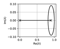
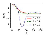
Since the pairs evolve independently, we can study their convergence by analyzing the eigenvalues of $\mathbf{A}$. Given that $\eta$ and $\beta$ are from the ranges defined in Sec. 3, all eigenvalues are strictly inside the right half of the complex unit circle which guarantees convergence to the ground truth. For step sizes $1<\eta<2$ eigenvalues will still be inside the complex unit circle, still guaranteeing convergence, but eigenvalues can be real and negative. This means that parameters will alternate signs every gradient update, denoted “ripples” [34]. Although this sign-switching can cause dying ReLU in theory, in practice learning rates are usually $<1$.

We plot the eigenvalues of $\mathbf{A}$ in Figure 2 (left) for $\eta=0.1$ as $\beta$ increases from $0$, i.e. GD without momentum, towards $1$. We observe that the eigenvalues eventually become complex ($\beta\approx 0.7$) resulting in oscillation [34] (seen on the right side). The fraction $\frac{b}{\|\mathbf{w}\|}$, as we will show in Sec. 5, is a good measure of to what extent the ReLU is dying (smaller means dying), and hence we plot this quantity in particular. Note that the eigenvalues, and thus the behavior is entirely parameterized by the learning rate and momentum, and independent of $\gamma$. Thus, we can not adjust $\eta$ as a function of $\gamma$ to make the system behave as the case $\gamma=1$. We now continue by showing how these properties translate to the case of a ReLU activated unit.

5 Regression with single ReLU-unit

We now want to understand the behavior of regressing to Eq. (5) with the ReLU model in Eq. (9). As discussed in Sec. 3, we will approximate the gradients by considering the linear target function in Eq. 4. Although this target can not be fully recovered, the optimal solution is still the same, and gradients share similarities, as previously discussed. Again, we consider the evolution and convergence of parameters $\boldsymbol{\theta}$ and momentum $\mathbf{m}$ during GD optimization, and assume that the inputs are distributed as $\mathbf{x}\sim\mathcal{N}(\mathbf{0};\mathbf{I})$ in the training data.

Similarity to affine model.

The ReLU will output non-zero values for any ${\mathbf{x}}$ that satisfies $\mathbf{w}^{\top}{\mathbf{x}}+b>0$. We can equivalently write this condition as

$$\frac{\mathbf{w}^{\top}}{\|\mathbf{w}\|}{\mathbf{x}} >-\frac{b}{\|\mathbf{w}\|}.$$ (21)

We can further simplify the condition from Eq. (21) using $\mathbf{U}$ from Sec. 3, which lets us consider the constraint solely in the $L$-th dimension

$$\footnotesize\frac{\mathbf{w}^{\top}}{\|\mathbf{w}\|}\mathbf{U}^{\top}\mathbf{U}{\mathbf{x}}>-\frac{b}{\|\mathbf{w}\|}\Rightarrow\frac{\tilde{\mathbf{w}}^{\top}}{\|\mathbf{w}\|}\tilde{\mathbf{x}}>-\frac{b}{\|\mathbf{w}\|}\Rightarrow[\tilde{\mathbf{x}}]_{L}>-\frac{b}{\|\mathbf{w}\|}.$$ (22)

From our assumption about the distribution of training inputs follows that $[\tilde{\mathbf{x}}]_{L} \sim\mathcal{N}(0,1)$.

With this result, we can compute the probability of a non-zero output from the ReLU as

$$\footnotesize P([\tilde{\mathbf{x}}]_{L}>-\frac{b}{\|\mathbf{w}\|})=1-P\left([\tilde{\mathbf{x}}]_{L}<-\frac{b}{\|\mathbf{w}\|}\right)=\Phi\left(\frac{b}{\|\mathbf{w}\|}\right),$$ (23)

where $\Phi$ is the cumulative distribution function (CDF) of the standard normal distribution.

Using Eq. (15), we see that dead ReLU is equivalent of $\Phi\left(\frac{b}{\|\mathbf{w}\|}\right)<\varepsilon$. This is equivalent of $\frac{b}{\|\mathbf{w}\|}<-\Phi^{-1}(\varepsilon)$ which defines a “dead” cone in parameter space. We can also formulate a corresponding “linear” cone. In this case we get $\frac{b}{\|\mathbf{w}\|}>\Phi^{-1}(\varepsilon)$ which is the same cone mirrored along the $b$-axis. In the linear cone, because of the similarity to the affine model, we know that parameters evolve as described in Sec. 4 with increased oscillations as momentum is used. We will now investigate the analytical gradients to see how these properties translate into that perspective.

Analytic gradients.

By inserting $\hat{y}_{f}$ into Eq. (10), the optimization objective can be formulated as

$${\mathcal{L}}(\boldsymbol{\theta}) =\mathbb{E}_{\mathbf{x}}\left[{\frac{1}{2}\mathbbm{1}_{\mathbf{w}^{\top}{\mathbf{x}}+b>0}(\mathbf{a}^{\top}{\mathbf{x}}+c)^{2}}\right],$$ (24)

where we use the indicator function $\mathbbm{1}_{\mathbf{w}^{\top}{\mathbf{x}}+b>0}$ to model the ReLU activation. The derivatives are

$$\frac{\partial{\mathcal{L}}}{\partial\mathbf{w}}=\mathbb{E}_{\mathbf{x}}\left[{\mathbbm{1}_{\mathbf{w}^{\top}{\mathbf{x}}+b>0}(\mathbf{a}^{\top}{\mathbf{x}}+c){\mathbf{x}}}\right]$$ (25)

for the weights and

$$\frac{\partial{\mathcal{L}}}{\partial b}=\mathbb{E}_{\mathbf{x}}\left[{\mathbbm{1}_{\mathbf{w}^{\top}{\mathbf{x}}+b>0}(\mathbf{a}^{\top}{\mathbf{x}}+c)}\right]$$ (26)

for the bias. As in Sec. 4, the optimal fit is given by weights $\mathbf{w}=\boldsymbol{\Gamma}$ and bias $b=\Delta$. These parameters give $\mathbf{a}=\mathbf{0}$ and $c=0$ and set the gradients in Eq. (25) and Eq. (26) to zero.

By changing base using $\mathbf{U}$, we can compute the derivatives,

$$\left[\mathbf{U}\frac{\partial\mathcal{L}}{\partial\mathbf{w}}\right]_{i\neq L}=[\tilde{\mathbf{a}}]_{i\neq L}\Phi\left(\frac{b}{\|\mathbf{w}\|}\right)$$ (27)

for the weights in dimensions $i\neq L$, and

$$\left[\mathbf{U}\frac{\partial\mathcal{L}}{\partial\mathbf{w}}\right]_{L}=[\tilde{\mathbf{a}}]_{L}\Phi\left(\frac{b}{\|\mathbf{w}\|}\right)+\left(c-[\tilde{\mathbf{a}}]_{L}\frac{b}{\|\mathbf{w}\|}\right)\phi\left(\frac{b}{\|\mathbf{w}\|}\right).$$ (28)

for dimension $L$, where we used $\phi$ as density function of the standard normal distribution. For the bias $b$ we have

$$\frac{\partial\mathcal{L}}{\partial b}=[\tilde{\mathbf{a}}]_{L}\phi\left(\frac{b}{\|\mathbf{w}\|}\right)+c\ \Phi\left(\frac{b}{\|\mathbf{w}\|}\right).$$ (29)

Full derivations are listed in Appendix B.

Critical points in parameter space.

With the gradients from above, we can analyze the possible parameters (i.e. optima and saddle points) to which GD can converge when the derivatives are zero. First of all, global optimum is easily verified to have gradient zero when $\tilde{\mathbf{a}}=\mathbf{a}=\mathbf{0}$ and $c=0$.

Saddle points correspond to dead ReLU and occur when $\frac{b}{\|\mathbf{w}\|}\rightarrow-\infty$ since then $\Phi(\frac{b}{\|\mathbf{w}\|})=0$, $\phi(\frac{b}{\|\mathbf{w}\|})=0$, and $\frac{b}{\|\mathbf{w}\|}\phi(\frac{b}{\|\mathbf{w}\|})\rightarrow 0$. This equals the case that $\mathbf{w}=\mathbf{0}$ for any $b<0$ which can be verified by plugging these values into Eq. (24). These saddle points form the center of the dead cone. Note in practice that these limits in practice occur already at, for example $\frac{b}{\|\mathbf{w}\|}=\pm 4$, since then $\phi(\pm 4)\approx 10^{-4}$. The implication of this is that an entire dead cone can be considered as saddle points in practice, and that parameters will converge on the surface of the cone rather than in its interior.

For $b>0$, we instead have $\frac{b}{\|\mathbf{w}\|}\rightarrow\infty$ and thus $\phi(\frac{b}{\|\mathbf{w}\|})=0$ and $\Phi(\frac{b}{\|\mathbf{w}\|})=1$ and the gradients can be verified to equal those of the affine model in Sec. 4, as expected. This verifies that parameter evolution in the linear cone will be approximately identical to the affine model.

Simplification to enable visualization.

To continue our investigation of the parameter evolution and, in particular, focus on how the target variance $\gamma$ and momentum evolve parameters into the dead cone we will make some simplifications. For this, we will assume that $[\tilde{\mathbf{a}}]_{i\neq L}=0$ which enables us to express gradients without $\mathbf{U}$ as

$$\frac{\partial\mathcal{L}}{\partial[\mathbf{w}]_{i\neq L}}=0.$$ (30)

For the weight $[\mathbf{w}]_{L}$ we can prove, see Appendix C, that

$$\footnotesize\frac{\partial\mathcal{L}}{\partial[\mathbf{w}]_{L}}=[\mathbf{a}]_{L}\Phi\left(\frac{b}{\|\mathbf{w}\|}\right)+\rho\left(c-\rho[\mathbf{a}]_{L}\frac{b}{\|\mathbf{w}\|}\right)\phi\left(\frac{b}{\|\mathbf{w}\|}\right),$$ (31)

where $\rho=\mathrm{sign}([\mathbf{w}]_{L})$ and $[\mathbf{a}]_{L}=[\mathbf{w}]_{L}-\gamma$. For the bias $b$ we get

$$\frac{\partial\mathcal{L}}{\partial b}=\rho[\mathbf{a}]_{L}\phi\left(\frac{b}{\|\mathbf{w}\|}\right)+c\ \Phi\left(\frac{b}{\|\mathbf{w}\|}\right).$$ (32)

This means, if all $[\tilde{\mathbf{a}}]_{i}=0$ for $i\neq L$, then only the weight $[\mathbf{w}]_{L}$ and bias $b$ evolve. We can now plot the vector fields in these parameters to see how they change w.r.t. $\gamma$.

Influence of $\gamma$ on convergence without momentum.

Figure 3: Parameter evolution from GD. The white dot marks the global optimum. Approaching $[\mathbf{w}]_{L}=0$ in the lower half, gradient norm becomes very small, GD gets stuck , and the ReLU dies.

The first key take-away when decreasing $\gamma$ is that the global optimum will be closer to the origin and eventually between the dead and the linear cone. This location of the optimum is particularly sensitive, since in this case the parameters in the linear cone evolve towards the dead cone, and in addition exhibits oscillatory behavior for large $\beta$. The color scheme in Figure 3 verifies that, like the probability of non-zero outputs in the dead cone, the gradients also tend to zero there. In the lower right quadrant, we can see an attracting line that is shifted towards the dead cone as $\gamma$ decreases, eventually ending up inside the dead cone. For this case, when $\gamma=0.001$, we can follow the lines to see that most parameters originating from the right side end up in the dead cone. Parameters originating in and near the linear cone approach the ground truth, and the lower left quadrant evolves first towards the linear cone before evolving towards the ground truth.

When adding momentum, remember that parameter evolution in and near the linear cone exhibits oscillatory behavior. The hypothesis at this moment is that parameters originating from the linear cone can oscillate over into the dead cone and get stuck there. For the other regions they either evolve as before into the dead cone, or first into the linear cone and then into the dead cone by oscillation. We will now evaluate and visualize this.

Regions that converge to global optimum.

We are interested in distinguishing the regions from which parameters will converge to the global optimum and dead cone respectively. For this, we apply the update rules, Eqs. (6) and (7), with $\eta=0.1$, until updates are smaller (in norm) than $10^{-6}$.

Figure 4: Parameter evolution from GD without momentum. Global optimum is shown as a white circle. The yellow dots correspond to initial parameter coordinates that converge at the ground truth. The blue dots all converge in the dead cone (where they stop are depicted as black dots). As can be seen, small target variance $\gamma$ is not alone sufficient to lead to a majority of dying ReLU.

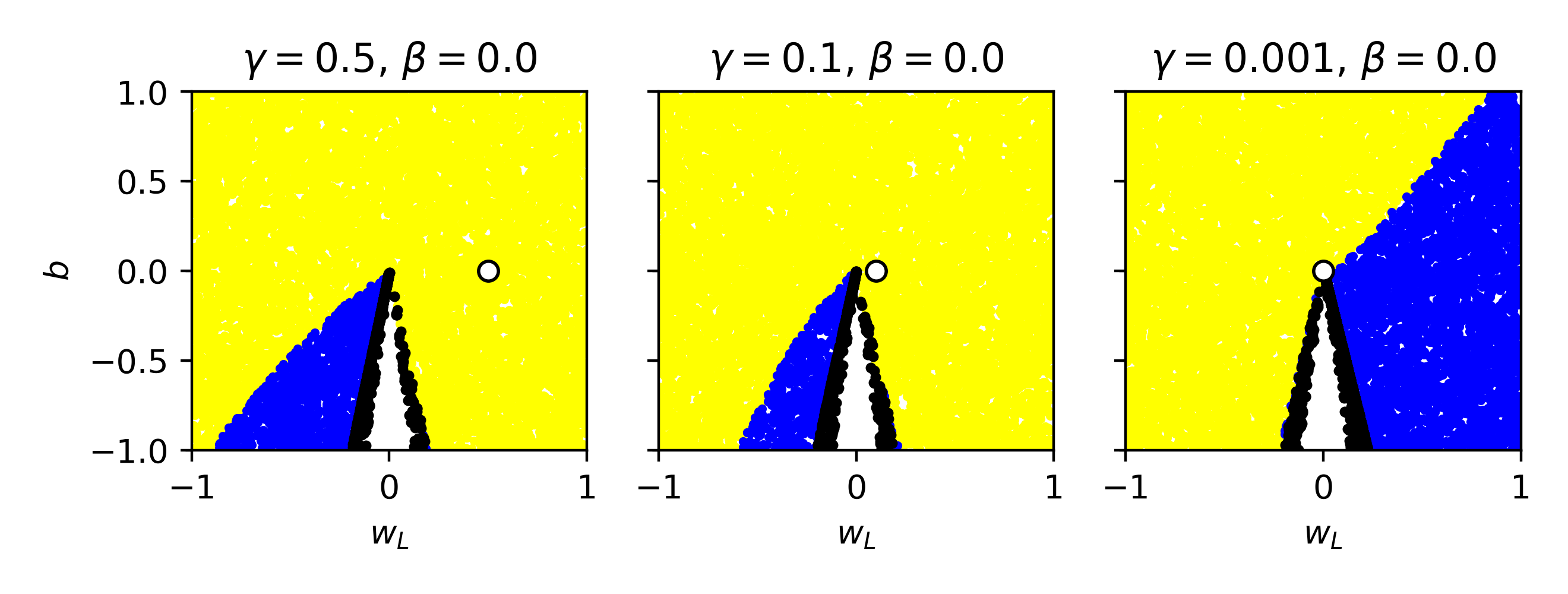
Figure 4 shows the results for GD without momentum ($\beta=0$). We see that the region that converges to the dead cone changes with $\gamma$, and eventually switches sign, when $\gamma$ becomes small. The majority of initializations still converges at the ground truth.

Figure 5: Parameter evolution from GD without momentum. Colors as in Figure 4. Momentum and small scale $\gamma=0.001$ increasingly leads to dying ReLU. The black regions corresponding to converged parameters are growing in the interior of the dead cone.

Figure 5 shows the results with momentum. The linear autonomous system in Sec. 4 with $\eta=0.1$ has complex eigenvalues for $\beta>0.7$ which lead to oscillation. This property approximately translates to the ReLU in the linear cone, where we expect oscillations for $\beta>0.7$. Indeed, we observe the same results as without momentum for $\beta\leq 0.7$, but worse results for larger $\beta$. Eventually, only small regions of initializations are able to converge to the global optimum.

6 Deeper architectures

In this section we will address two questions. (1) Does the problem persist in deeper architectures, including residual networks with batch normalization? (2) Since the ReLU is a linear operator for positive coefficients, can we simply scale the weight initialization and learning rate and have an equivalent network and learning procedure? For the latter we will show that it is not possible for deeper architectures.

Relevance for models used in practice.

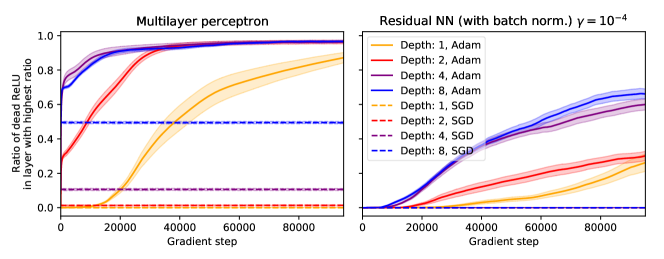
We performed regression on the same datasets as in Sec. 1, with $\gamma=10^{-4}$. We confirm the findings of Lu et al. [13] that ReLUs are initialized dead in deeper “vanilla” NNs, but not in residual networks due to the batch normalization layer that precedes the ReLU. Results are shown in Figure 6. We further find that ReLUs die more often, and faster, the deeper the architecture, even for residual networks with batch normalization. We can also conclude that, in these experiments, stochastic gradient descent does not produce more dead ReLU during optimization.

Figure 6: Average results over four datasets showing that dead ReLU is aggravated by deeper architectures, even for residual networks with batch normalization before the ReLU activation. Horizontal axis shows the proportion of dead ReLU in the layer with the highest ratio of dead ReLU. In the multi-layer perceptron case, if one layer has only dead ReLUs, then gradients are zero for all parameters except the last biases, no matter which layer “died”.

Parameter re-scaling.

For $\gamma>0$, the ReLU function has the property $f(\gamma{\mathbf{x}})=\gamma f({\mathbf{x}})$ and thus $\gamma\hat{y}({\mathbf{x}})=f(\gamma\mathbf{w}^{\top}{\mathbf{x}}+\gamma b)$. By rescaling the weight and bias initializations (not learning rate) by $\gamma$, the parameter trajectories during learning will proportional no matter the choice of $\gamma>0$. That is, ReLUs will die independent of $\gamma$. This is a special case though, since for any architecture $\hat{y}$ with one or more hidden layers, it is not possible to multiply parameters by a single scalar $\nu$ such that the function is identical to $\gamma\hat{y}$. Proof is provided in Appendix D. Also, we still have a problem if we do not know $\gamma$ in advance, which holds for example in the reinforcement learning setting.

7 Conclusion and future work

Target normalization is indeed a well-motivated and used practice, although we believe a theoretical understanding of why is both important and lacking. We take a first stab at the problem by understanding the properties in the smallest moving part of a neural network, a single ReLU-activated affine transformation. Gradient descent on parameters of an affine transformation can be expressed as a discrete-time linear system, for which we have tools to explain the behavior. We provide a geometrical understanding of how these properties translate to the ReLU case, and when it is considered dead. We further illustrated that weight initialization from large regions in parameter space lead to dying ReLUs as target variance is decreased along with momentum optimization, and show that the problem is still relevant, and even aggravated, for deeper architectures. Remaining questions to be answered include how we can extend the analysis for the single ReLU to the full network. Here, the implicit target function of the single ReLU is likely neither of the linear or piecewise linear functions, and inputs are not Gaussian distributed and vary over time.

Appendix A Regression experiment details

NN used for regression was of the form

$$\hat{y}({\mathbf{x}})=\mathbf{w}^{\top}\sigma(W{\mathbf{x}}+b^{(1)})+b^{(2)}$$ (33)

where $\mathbf{w}\in{\mathbb{R}}^{200\times 1}$ and $W\in{\mathbb{R}}^{200\times n}$ where $n$ is the dimensionality of the input data. All elements in $W$ and $b^{(1)}$ were initialized from $U(-\frac{1}{\sqrt{n}},\frac{1}{\sqrt{n}})$. The elements of $\mathbf{w}$ and $b^{(2)}$ were initialized from $U(-\frac{1}{\sqrt{200}},\frac{1}{\sqrt{200}})$. Batch size was $64$ and the Adam optimizer was set to use the same parameters as suggested by [6]. Every experiment was run $8$ times with different seeds, effecting the random ordering of mini-batches and initialization of parameters. Each experiment was allowed $250000$ gradient updates before evaluation. Evaluation was performed on a subset of the training set, as we wanted to investigate the fit to the data rather than generalization.

Appendix B Single ReLU gradients

For brevity we will use $\mathbbm{1}$ in place of $\mathbbm{1}_{\tilde{x}_{L}>-\frac{b}{\|\mathbf{w}\|}}$ below. Subscript notation on non-bold symbols here represents single dimensions of the vector counterpart. The gradient w.r.t. $\mathbf{w}$ is

$$\frac{\partial{\mathcal{L}}}{\partial\mathbf{w}} =\mathbb{E}_{\mathbf{x}}\left[{\mathbbm{1}_{\mathbf{w}^{\top}{\mathbf{x}}+b>0}(\mathbf{a}^{\top}{\mathbf{x}}+c){\mathbf{x}}}\right]$$

$$=\mathbb{E}_{\mathbf{x}}\left[{\mathbbm{1}_{\mathbf{w}^{\top}U^{\top}U{\mathbf{x}}+b>0}(\mathbf{a}^{\top}U^{\top}U{\mathbf{x}}+c)U^{\top}U{\mathbf{x}}}\right]$$

$$=U^{\top}\mathbb{E}_{\tilde{\mathbf{x}}}\left[{\mathbbm{1}(\tilde{\mathbf{a}}^{\top}\tilde{\mathbf{x}}+c)\tilde{\mathbf{x}}}\right]$$

Multiplying by $U$ from the left and looking at a dimension $i\neq L$, we get:

$$\left[U\frac{\partial{\mathcal{L}}}{\partial\mathbf{w}}\right]_{i} = \mathbb{E}_{\tilde{\mathbf{x}}}\left[{\mathbbm{1}(\tilde{\mathbf{a}}^{\top}\tilde{\mathbf{x}}+c)\tilde{x}_{i}}\right]$$

$$= \mathbb{E}_{\tilde{\mathbf{x}}}\left[{\mathbbm{1}\left(\tilde{x}_{i}\left(\sum_{j\neq i}^{L}\tilde{a}_{j}\tilde{x}_{j}+c\right)+\tilde{a}_{i}\tilde{x}_{i}^{2}\right)}\right]$$

$$= \underbrace{\mathbb{E}_{\tilde{\mathbf{x}}}\left[{\mathbbm{1}\tilde{x}_{i}}\right]}_{=0}\mathbb{E}_{\tilde{\mathbf{x}}}\left[{\mathbbm{1}\left(\sum_{j\neq i}^{L}\tilde{a}_{j}\tilde{x}_{j}+c\right)}\right]$$

$$+\tilde{a}_{i}\mathbb{E}_{\tilde{\mathbf{x}}}\left[{\mathbbm{1}\tilde{x}_{i}^{2}}\right]$$

$$= \tilde{a}_{i}\underbrace{\text{Var}(\tilde{x}_{i})}_{=1}\mathbb{E}_{\tilde{x}_{L}}\left[\mathbbm{1}\right]$$

$$= \tilde{a}_{i}\Phi\left(\frac{b}{\|\mathbf{w}\|}\right)$$

For $i=L$ we instead have

$$\left[U\frac{\partial{\mathcal{L}}}{\partial\mathbf{w}}\right]_{L} = \mathbb{E}_{\tilde{\mathbf{x}}}\left[{\mathbbm{1}(\tilde{\mathbf{a}}^{\top}\tilde{\mathbf{x}}+c)\tilde{x}_{L}}\right]$$

$$= \mathbb{E}_{\tilde{\mathbf{x}}}\left[{\mathbbm{1}\left(\tilde{x}_{L}\sum_{j=1}^{L-1}\tilde{a}_{j}\tilde{x}_{j}+\tilde{a}_{L}\tilde{x}_{L}^{2}+c\tilde{x}_{L}\right)}\right]$$

$$= \mathbb{E}_{\tilde{\mathbf{x}}}\left[{\mathbbm{1}\tilde{x}_{L}}\right]\left(\sum_{j=1}^{L-1}\tilde{a}_{j}\underbrace{\mathbb{E}_{\tilde{\mathbf{x}}}\left[{\mathbbm{1}\tilde{x}_{j}}\right]}_{=0}\right)$$

$$+\tilde{a}_{L}\mathbb{E}_{\tilde{\mathbf{x}}}\left[{\mathbbm{1}\tilde{x}_{L}^{2}}\right]$$

$$+c\mathbb{E}_{\tilde{\mathbf{x}}}\left[{\mathbbm{1}\tilde{x}_{L}}\right]$$ (34)

We can calculate the second term with integration by parts

$$\mathbb{E}_{\tilde{\mathbf{x}}}\left[{\mathbbm{1}\tilde{x}_{L}^{2}}\right] = \frac{1}{\sqrt{2\pi}}\int\limits_{-\frac{b}{\|\mathbf{w}\|}}^{\infty}\tilde{x}_{L}\cdot\tilde{x}_{L}e^{-\frac{\tilde{x}_{L}^{2}}{2}}d\tilde{x}_{L}$$

$$= \frac{1}{\sqrt{2\pi}}\left[-\tilde{x}_{L}e^{-\frac{\tilde{x}_{L}^{2}}{2}}\right]_{-\frac{b}{\|\mathbf{w}\|}}^{\infty}$$

$$+\frac{1}{\sqrt{2\pi}}\int\limits_{-\frac{b}{\|\mathbf{w}\|}}^{\infty}e^{-\frac{\tilde{x}_{L}^{2}}{2}}d\tilde{x}_{L}$$

$$= -\frac{b}{\|\mathbf{w}\|}\phi\left(\frac{b}{\|\mathbf{w}\|}\right)+\Phi\left(\frac{b}{\|\mathbf{w}\|}\right)$$

The third term:

$$\int\limits_{-\frac{b}{\|\mathbf{w}\|}}^{\infty}\frac{\tilde{x}_{L}}{\sqrt{2\pi}}e^{-\frac{\tilde{x}_{L}^{2}}{2}} =-\left[\frac{1}{\sqrt{2\pi}}e^{-\frac{\tilde{x}_{L}^{2}}{2}}\right]_{-\frac{b}{\|\mathbf{w}\|}}^{\infty}$$

$$=-\left[\phi(\tilde{x}_{L})\right]_{-\frac{b}{\|\mathbf{w}\|}}^{\infty}$$

$$=\phi\left(\frac{b}{\|\mathbf{w}\|}\right).$$

By substituting these expressions back in to Eq. (34) and simplifying we get Eq. (28). The derivation of gradients w.r.t. the bias is very similar to the gradients w.r.t. to $\mathbf{w}$ and are omitted here for brevity.

Appendix C Gradients after convergence in the $(L-1)$ first dimensions

If we assume the $L-1$ first dimensions of $\tilde{a}$ are zero, we can show that the $L-1$ first dimensions of $\mathbf{w}$ all have gradient zero. We can then also express the gradient without the unitary matrix $U$ that otherwise needs to be calculated for every new $\mathbf{w}$. We present this as a proposition by the end of this section. First, we need to show some preliminary steps.

Lemma C.1.

If

$$\tilde{\mathbf{a}}=(0,...,0,\tilde{a}_{L})^{\top}$$

then

$$U\Gamma=(0,...,0,k\gamma)^{\top}$$

where $k$ is either $-1$ or $1$.

Proof.

As defined in Eq. (13), we have $U\mathbf{w}=(0,...,0,\|\mathbf{w}\|)^{\top}$. Since

$$\tilde{\mathbf{a}} =U\mathbf{a}$$

$$=U\mathbf{w}-U\Gamma$$

$$=(0-[U\Gamma]_{1},...,0-[U\Gamma]_{L-1},\|\mathbf{w}\|-[U\Gamma]_{L})$$

we must have $U\Gamma=(0,...,0,\ell)^{\top}$. Since U is unitary we must have $|\ell|=\gamma$ which is solved by $\ell=\pm\gamma$. ∎

Lemma C.2.

If

$$\tilde{\mathbf{a}}=(0,...,0,\tilde{a}_{L})^{\top}$$

then

$$\mathbf{w}=(0,...,0,w_{L})^{\top}$$

Proof.

We have from Lemma C.1 that $\Gamma$ and $U\Gamma$ lie in the same one-dimensional linear subspace $\mathcal{K}$ spanned by $(0,...,1)^{\top}$. Since $U$ is unitary and $U\mathbf{w}$ also is in $\mathcal{K}$, then so must $\mathbf{w}$. This implies that $\mathbf{w}=(0,0,...,0,w_{L})^{\top}$. ∎

Lemma C.3.

If

$$\tilde{\mathbf{a}}=(0,...,0,\tilde{a}_{L})^{\top}$$

then for any vector $\mathbf{v}$ in the linear subspace $\mathcal{K}$ spanned by $(0,0,...,1)^{\top}$ we have

$$U\mathbf{v}=U^{\top}\mathbf{v}=\rho\mathbf{v}$$

where $\rho=\mathrm{sign}(w_{L})$.

Proof.

From Lemma C.2, we have $\mathbf{w}=(0,...,0,w_{L})^{\top}$, which implies $\frac{\mathbf{w}}{\|\mathbf{w}\|}=(0,...,0,\rho)^{\top}$. By the property of $U$ as defined in Eq. (13) we have

$$U\frac{\mathbf{w}}{\|\mathbf{w}\|}=(0,...,0,1)^{\top}.$$

Multiplying by $U^{\top}$ from the left, we have

$$U^{\top}U\frac{\mathbf{w}}{\|\mathbf{w}\|} =U^{\top}(0,...,0,1)^{\top}$$

$$=(0,...,0,\rho)^{\top}$$

This implies that the last row and last column of $U$ is $(0,...,0,\rho)$. Then

$$U\mathbf{v} =U(0,...,0,v_{L})^{\top}$$

$$=(0,...,0,\rho v_{L})^{\top}$$

$$=\rho\mathbf{v}$$

Since the last row and last column are the same for $U$, the above also holds for the transpose $U^{\top}$. ∎

Proposition C.1.

If

$$\tilde{\mathbf{a}}=(0,...,0,\tilde{a}_{L})^{\top}$$

then

$$\frac{\partial\mathcal{L}}{\partial w_{L}}=a_{L}\Phi(\frac{b}{\|w\|})+\rho(c-\rho a_{L}\frac{b}{\|w\|})\phi(\frac{b}{\|w\|})$$

and

$$\frac{\partial\mathcal{L}}{\partial w_{i}}=0$$

for $i\neq L$ and where $\rho=\mathrm{sign}(w_{L})$ and $a_{L}=w_{L}-\gamma$. The gradient w.r.t. the bias is

$$\frac{\partial\mathcal{L}}{\partial b}=\rho a_{L}\phi(\frac{b}{\|w\|})+c\Phi(\frac{b}{\|w\|}).$$

Proof.

From Lemma C.1 and C.3 we have that

$$U\mathbf{a}=U(0,0,...,0,w_{L}-\gamma)^{\top}=(0,0,...,0,\rho(w_{L}-\gamma))^{\top}$$

and therefore $\tilde{a}_{L}=\rho a_{L}$. All occurrences of $\tilde{a}_{L}$ can now be replaced with this quantity. The rotated gradient is

$$U\frac{\partial\mathcal{L}}{\partial w}=(0,0,...,0,\xi)^{\top}\in\mathcal{K}$$

where $\xi$ is given by Eq. (28). Hence $\frac{\partial\mathcal{L}}{\partial w}=U^{\top}\left(U\frac{\partial\mathcal{L}}{\partial w}\right)=(0,0,...,0,\rho\xi)^{\top}$ by Lemma C.3. ∎

Appendix D Scaling of parameters

Before stating the problem, we define an N-hidden layer neural network recursively

$$\hat{y}({\mathbf{x}})=\mathbf{w}^{\top}y^{(N)}({\mathbf{x}})+b$$ (35)

where

$$y^{(n)}({\mathbf{x}})=f(W^{(n)}y^{(n-1)}+\mathbf{b}^{(n)})$$ (36)

and

$$y^{(0)}({\mathbf{x}})={\mathbf{x}}.$$ (37)

Denote the joint collection of parameters $\mathbf{w}$, $b$, $\{W^{(n)}\}_{i=1}^{N}$ and $\{\mathbf{b}^{(n)}\}_{i=1}^{N}$ as $\theta$. We denote $\hat{y}({\mathbf{x}})=\hat{y}({\mathbf{x}},\theta)$ to make explicit the dependence on $\theta$. We now investigate whether a scaling of $\hat{y}$ can be achieved by scaling all parameters by a single number.

Theorem D.1.

Given some $\gamma>0$, $\gamma\neq 1$, there exists no $\nu>0$ such that

$$\gamma\hat{y}({\mathbf{x}},\theta)=\hat{y}({\mathbf{x}},\nu\theta)$$ (38)

Proof.

First, denote $\gamma=\gamma_{N+1}$ and factorize into $N+1$ factors $\alpha_{i}>0$

$$\gamma_{n}=\prod\limits_{i=1}^{n}\alpha_{i}.$$ (39)

Multiplying $\hat{y}$ by $\gamma$ gives:

$$\gamma\hat{y}({\mathbf{x}}) =\gamma_{N+1}\mathbf{w}^{\top}y^{(N)}({\mathbf{x}})+\gamma_{N+1}b$$ (40)

$$=\frac{\gamma_{N+1}}{\gamma_{N}}\mathbf{w}^{\top}\gamma_{N}y^{(N)}({\mathbf{x}})+\gamma_{N+1}b$$ (41)

$$=\alpha_{N+1}\mathbf{w}^{\top}\gamma_{N}y^{(N)}({\mathbf{x}})+\gamma_{N+1}b$$ (42)

and similarly

$$\gamma_{n}y^{(n)}({\mathbf{x}}) =\gamma_{n}f(W^{(n)}y^{(n-1)}({\mathbf{x}})+\mathbf{b}^{(n)})$$ (43)

$$=f(\alpha_{n}W^{(n)}\gamma_{n-1}y^{(n-1)}({\mathbf{x}})+\gamma_{n}\mathbf{b}^{(n)}).$$ (44)

We finally define $\gamma_{0}y^{(0)}({\mathbf{x}})=1\cdot{\mathbf{x}}$.

If a $\nu$ exists that satisfies Eq. (38), then we must have all $\alpha_{i}=\nu$. If $\gamma>1$, then $\gamma_{n}=\nu^{n}>\nu=\alpha_{n}$ and thus in Eqs. (42) and (44) the weights and biases are not multiplied by the same number $\gamma_{n}\neq\alpha_{n}$. Similarly, this holds for $\gamma<1$.

∎

References

- Dargan et al. [2019] Shaveta Dargan, Munish Kumar, Maruthi Rohit Ayyagari, and Gulshan Kumar. A survey of deep learning and its applications: A new paradigm to machine learning. Archives of Computational Methods in Engineering, 2019. ISSN 1134-3060.
- Rumelhart et al. [1986] David E Rumelhart, Geoffrey E Hinton, and Ronald J Williams. Learning representations by back-propagating errors. nature, 323(6088):533–536, 1986.
- Srivastava et al. [2015] Rupesh K Srivastava, Klaus Greff, and Jürgen Schmidhuber. Training very deep networks. In Advances in neural information processing systems, pages 2377–2385, 2015.
- Du et al. [2019] Simon Du, Jason Lee, Haochuan Li, Liwei Wang, and Xiyu Zhai. Gradient descent finds global minima of deep neural networks. In International Conference on Machine Learning, pages 1675–1685, 2019.
- Sutskever et al. [2013] Ilya Sutskever, James Martens, George Dahl, and Geoffrey Hinton. On the importance of initialization and momentum in deep learning. In International conference on machine learning, pages 1139–1147, 2013.
- Kingma and Ba [2015] Diederik P. Kingma and Jimmy Ba. Adam: A method for stochastic optimization. In 3rd International Conference on Learning Representations, ICLR 2015, San Diego, CA, USA, May 7-9, 2015, Conference Track Proceedings, 2015. URL http://arxiv.org/abs/1412.6980.
- LeCun et al. [2012] Yann A LeCun, Léon Bottou, Genevieve B Orr, and Klaus-Robert Müller. Efficient backprop. In Neural networks: Tricks of the trade, pages 9–48. Springer, 2012.
- LeCun et al. [2015] Yann LeCun, Yoshua Bengio, and Geoffrey Hinton. Deep learning. nature, 521(7553):436, 2015.
- Ramachandran et al. [2017] Prajit Ramachandran, Barret Zoph, and Quoc V Le. Searching for activation functions. arXiv preprint arXiv:1710.05941, 2017.
- Nair and Hinton [2010] Vinod Nair and Geoffrey E Hinton. Rectified linear units improve restricted boltzmann machines. In Proceedings of the 27th international conference on machine learning (ICML-10), pages 807–814, 2010.
- Glorot et al. [2011] Xavier Glorot, Antoine Bordes, and Yoshua Bengio. Deep sparse rectifier neural networks. In Proceedings of the fourteenth international conference on artificial intelligence and statistics, pages 315–323, 2011.
- Sun et al. [2015] Yi Sun, Xiaogang Wang, and Xiaoou Tang. Deeply learned face representations are sparse, selective, and robust. In Proceedings of the IEEE conference on computer vision and pattern recognition, pages 2892–2900, 2015.
- Lu et al. [2019] Lu Lu, Yeonjong Shin, Yanhui Su, and George Em Karniadakis. Dying relu and initialization: Theory and numerical examples. arXiv preprint arXiv:1903.06733, 2019.
- Trottier et al. [2017] Ludovic Trottier, Philippe Gigu, Brahim Chaib-draa, et al. Parametric exponential linear unit for deep convolutional neural networks. In 2017 16th IEEE International Conference on Machine Learning and Applications (ICMLA), pages 207–214. IEEE, 2017.
- Agarap [2018] Abien Fred Agarap. Deep learning using rectified linear units (relu). arXiv preprint arXiv:1803.08375, 2018.
- Maas et al. [2013] Andrew L Maas, Awni Y Hannun, and Andrew Y Ng. Rectifier nonlinearities improve neural network acoustic models. In Proc. icml, volume 30, page 3, 2013.
- Clevert et al. [2016] Djork-Arné Clevert, Thomas Unterthiner, and Sepp Hochreiter. Fast and accurate deep network learning by exponential linear units (elus). In 4th International Conference on Learning Representations, ICLR 2016, San Juan, Puerto Rico, May 2-4, 2016, Conference Track Proceedings, 2016.
- He et al. [2015] Kaiming He, Xiangyu Zhang, Shaoqing Ren, and Jian Sun. Delving deep into rectifiers: Surpassing human-level performance on imagenet classification. In 2015 IEEE International Conference on Computer Vision (ICCV), pages 1026–1034. IEEE, 2015.
- Ba et al. [2016] Jimmy Lei Ba, Jamie Ryan Kiros, and Geoffrey E Hinton. Layer normalization. arXiv preprint arXiv:1607.06450, 2016.
- Ioffe and Szegedy [2015] Sergey Ioffe and Christian Szegedy. Batch normalization: Accelerating deep network training by reducing internal covariate shift. arXiv preprint arXiv:1502.03167, 2015.
- Dua and Graff [2017] Dheeru Dua and Casey Graff. UCI machine learning repository, 2017. URL http://archive.ics.uci.edu/ml.
- Poole et al. [2016] Ben Poole, Subhaneil Lahiri, Maithra Raghu, Jascha Sohl-Dickstein, and Surya Ganguli. Exponential expressivity in deep neural networks through transient chaos. In Advances in neural information processing systems, pages 3360–3368, 2016.
- Hanin [2018] Boris Hanin. Which neural net architectures give rise to exploding and vanishing gradients? In Advances in Neural Information Processing Systems, pages 582–591, 2018.
- Wu et al. [2018] Yeah-Hua Wu, Fan-Yun Sun, Yen-Yu Chang, and Should-De Lin. Ans: Adaptive network scaling for deep rectifier reinforcement learning models. arXiv preprint arXiv:1809.02112, 2018.
- Sola and Sevilla [1997] J Sola and Joaquin Sevilla. Importance of input data normalization for the application of neural networks to complex industrial problems. IEEE Transactions on nuclear science, 44(3):1464–1468, 1997.
- Raiko et al. [2012] Tapani Raiko, Harri Valpola, and Yann LeCun. Deep learning made easier by linear transformations in perceptrons. In Artificial intelligence and statistics, pages 924–932, 2012.
- Klambauer et al. [2017] Günter Klambauer, Thomas Unterthiner, Andreas Mayr, and Sepp Hochreiter. Self-normalizing neural networks. In I. Guyon, U. V. Luxburg, S. Bengio, H. Wallach, R. Fergus, S. Vishwanathan, and R. Garnett, editors, Advances in Neural Information Processing Systems 30, pages 971–980. Curran Associates, Inc., 2017. URL http://papers.nips.cc/paper/6698-self-normalizing-neural-networks.pdf.
- Santurkar et al. [2018] Shibani Santurkar, Dimitris Tsipras, Andrew Ilyas, and Aleksander Madry. How does batch normalization help optimization? In Advances in Neural Information Processing Systems, pages 2483–2493, 2018.
- Glorot and Bengio [2010] Xavier Glorot and Yoshua Bengio. Understanding the difficulty of training deep feedforward neural networks. In Proceedings of the thirteenth international conference on artificial intelligence and statistics, pages 249–256, 2010.
- van Hasselt et al. [2016] Hado P van Hasselt, Arthur Guez, Matteo Hessel, Volodymyr Mnih, and David Silver. Learning values across many orders of magnitude. In Advances in Neural Information Processing Systems, pages 4287–4295, 2016.
- Henderson et al. [2018] Peter Henderson, Riashat Islam, Philip Bachman, Joelle Pineau, Doina Precup, and David Meger. Deep reinforcement learning that matters. In Thirty-Second AAAI Conference on Artificial Intelligence, 2018.
- Goldin and Kanellakis [1995] Dina Q Goldin and Paris C Kanellakis. On similarity queries for time-series data: constraint specification and implementation. In International Conference on Principles and Practice of Constraint Programming, pages 137–153. Springer, 1995.
- Douglas and Yu [2018] Scott C Douglas and Jiutian Yu. Why relu units sometimes die: Analysis of single-unit error backpropagation in neural networks. In 2018 52nd Asilomar Conference on Signals, Systems, and Computers, pages 864–868. IEEE, 2018.
- Goh [2017] Gabriel Goh. Why momentum really works. Distill, 2(4):e6, 2017.
Acknowledgements
This work was funded by the *********** through the project ************.