Boosting on the shoulders of giants in quantum device calibration

Abstract

Traditional machine learning applications, such as optical character recognition, arose from the inability to explicitly program a computer to perform a routine task. In this context, learning algorithms usually derive a model exclusively from the evidence present in a massive dataset. Yet in some scientific disciplines, obtaining an abundance of data is an impractical luxury, however; there is an explicit model of the domain based upon previous scientific discoveries. Here we introduce a new approach to machine learning that is able to leverage prior scientific discoveries in order to improve generalizability over a scientific model. We show its efficacy in predicting the entire energy spectrum of a Hamiltonian on a superconducting quantum device, a key task in present quantum computer calibration. Our accuracy surpasses the current state-of-the-art by over $20\%.$ Our approach thus demonstrates how artificial intelligence can be further enhanced by “standing on the shoulders of giants.”

Prediction is paramount in almost every branch of science. In studying and designing learning systems, we are interested in prediction performance on examples unencountered during training. As machines learn inductively, generalizing training examples into an accurate model requires some restriction on the search space of hypotheses, based upon prior knowledge Hume_1739 ; Haussler_1988 ; Mitchell_1991 ; Wolpert_1997 . The choice of hypothesis space constitutes the problem of inductive bias Haussler_1988 ; Mitchell_1991 ; Caruana_1997 ; Wolpert_1997 ; Baxter_2000 , which is of broad significance in scientific applications.

Some scientific applications, such as quantum experiments, provide a paucity of data due to experimental cost, but compensate with an explicit model based upon previous discoveries Brunton_2016 ; Roushan_2017 ; Butler_2018 ; Neill_2018 ; Chiaro_2019 . In prior work, this prior knowledge has been disregarded, and research has focused on entirely data-driven approaches that reproduce major scientific achievements or learn from toy data Schmidt_2009 ; Carrasquilla_2017 ; Melnikov_2018 ; Koch-Janusz_2018 ; Torlai_2018 ; Wu_2019 ; Iten_2020 ; Wetzel_2020 . This leads us to ask if a machine learner can leverage prior scientific knowledge in order to outperform contemporary researchers? Particularly in scenarios with a shortage of experimental data.

Here, we introduce a new framework that restricts a learning algorithm’s search space of hypotheses. It does so by leveraging prior knowledge contained in predictions generated by a scientific model (see Fig. 2).

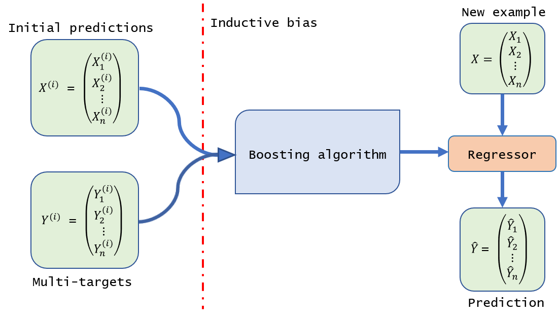
Figure 1: Conceptual representation of the learning framework. Given a base regressor’s initial multi-target predictions and the multi-target observations, we wrangle this data for multi-target supervised learning Borchani_2015 ; Waegeman_2019 . Next, the boosting algorithm receives the training examples and acquires an inductive bias from the initial predictions. This compensates for a shortage of training examples, and the boosting algorithm improves generalizability over the base regressor. Given a new example, the boosting algorithm’s returned regressor predicts a real vector.

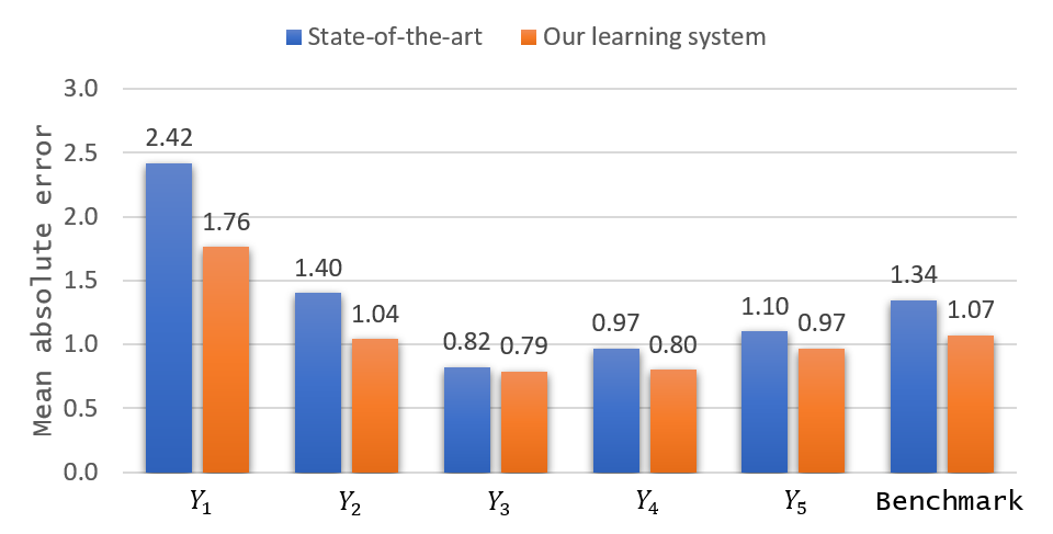
Figure 2: Benchmark task. Using the learning framework in Fig. 2, our learning system surpasses the state-of-the-art Roushan_2017 ; Neill_2018 ; Chiaro_2019 by over $20\%$ on the calibration task of simultaneously predicting the entire energy spectrum of a Hamiltonian Eq. 1 on a nearest-neighbor coupled linear chain of superconducting qubits. Moreover, our learning system outperforms the state-of-the-art on each individual prediction task, i.e., $Y_{j},$ where $j\in\{1,2,\dots,5\}.$

In contrast to conventional supervised learning, we focus on the simultaneous prediction of multiple real variables, which is known as multi-target regression Caruana_1997 ; Sklearn_2011 ; Borchani_2015 ; Waegeman_2019 . This enables the learning algorithm to improve generalizability over the scientific model by discovering relationships among the targets, which the model did not envisage. In principle, this approach shares similarities with neuroplasticity, whereby the nervous system is able to adapt and optimize its limited resources in response to sensory experiences Pascual_leone_2005 .

To test our learning system, we establish a proxy of expert human-level performance on the calibration benchmark task of simultaneously predicting the entire energy spectrum of a Hamiltonian on a superconducting quantum device Chen_2014 ; Roushan_2017 ; Neill_2018 ; Chiaro_2019 . In this scenario, there is a shortage of data due to operational cost of the experiment Roushan_2017 . The explicit scientific model of the device’s quantum behavior is state-of-the-art Roushan_2017 ; Neill_2018 ; Chiaro_2019 . We demonstrate that our learning system surpasses this baseline of expert human-level performance by over $20\%$ (see Fig. 2). Consequently, we advance the current ability to precisely generate Hamiltonians with programmable parameters for a variety of quantum simulation applications. Our result complements other recent applications of machine learning in scientific settings, and more specifically quantum systems Schmidt_2009 ; Zahedinejad_2016 ; Brunton_2016 ; Lin_2017 ; Biamonte_2017 ; Carrasquilla_2017 ; Koch-Janusz_2018 ; Torlai_2018 ; Butler_2018 ; Melnikov_2018 ; Dunjko_2018 ; Wu_2019 ; Giuseppe_2019 ; Mehta_2019 ; Iten_2020 ; Wetzel_2020 ; Udrescu_2020 . To interpret our results we use techniques from explainable machine learning Lundberg_2017 ; Molnar_2020 to uncover parameter dependencies in the original scientific model.

Results

Benchmark task – In order to establish a proxy of expert human-level performance for the analysis of our learning system, we study a superconducting qubit architecture Chen_2014 . The quantum device is a nearest-neighbor coupled linear chain of superconducting qubits with tunable qubit frequencies and tunable inter-qubit interactions Chen_2014 ; Roushan_2017 ; Neill_2018 ; Chiaro_2019 . Each qubit is embedded in the subspace spanned by the ground state and first excited state of a nonlinear photonic resonator in the microwave regime. The total Hamiltonian of the device is approximately described by the Bose-Hubbard model truncated at two local excitations

$$\begin{split}\mathcal{H}&=\sum_{j=1}^{n}\delta_{j}\hat{a}^{\dagger}_{j}\hat{a}_{j}+\frac{L}{2}\hat{a}^{\dagger}_{j}\hat{a}_{j}(\hat{a}^{\dagger}_{j}\hat{a}_{j}-1)\\ &+\sum_{j=1}^{n-1}g_{j,j+1}(\hat{a}^{\dagger}_{j}\hat{a}_{j+1}+\hat{a}_{j}\hat{a}^{\dagger}_{j+1}),\end{split}$$ (1)

where $n>1$ is the number of qubits, $\hat{a}^{\dagger}$ ($\hat{a}$) is the bosonic creation (annihilation) operator, $\delta_{j}$ is the random on-site detuning, $L$ is the on-site Hubbard interaction, and $g_{j,j+1}$ is the hopping rate between nearest neighbor lattice sites. Quantum evolution is typically realized by allowing the entire system to interact at once, which also admits translation into the prototypical quantum circuit model Neill_2018 .

In the benchmark task, the device contains $9$ qubits. The $n=5$ rightmost qubits and $4$ interleaving couplers were utilized during experimentation, while the $4$ leftmost qubits and couplers were left idle. The device is being calibrated for a many-body localization experiment Roushan_2017 ; Chiaro_2019 , where different relaxation dynamics are observed, depending on the extent of random disorder in the system. Probing this quantum phenomenon requires study of the entire energy spectrum, which be achieved experimentally through many-body Ramsey spectroscopy Roushan_2017 .

Here, we focus on the identification of $5$ eigenenergies belonging to Eq. 1, when it describes hopping of a single photon in a disordered potential. The energy eigenstates are generally not local and each instance of the many-body Ramsey spectroscopy technique sorts the measured eigenenergies in ascending order: $Y_{1},Y_{2},\dots,Y_{5}.$ In the present context of machine learning, we refer to these variables as single-targets and to their collection as a multi-target (details in Methods).

The calibration is performed in two steps Roushan_2017 ; Neill_2018 ; Chiaro_2019 , where the benchmark dataset pertains to the second step. In the first step, the room temperature time-dependent pulses that orchestrate the computation are calibrated to arrive at the device: orthogonally, synchronously, and without pulse-distortion Neill_2018 . In the second step, the control pulses are converted to matrix elements of the Hamiltonian Eq. 1. Underlying this conversion is a finitely parameterized model of the device’s electronic circuitry, which is directly encoded in the classical control program Roushan_2017 ; Neill_2018 ; Chiaro_2019 .

Inferring the physical parameters of the control model entails fitting the two lowest transition energies of each qubit as a function of qubit and coupler flux-biases Neill_2018 . Next, the many-body Ramsey spectroscopy technique benchmarks the collective dynamics of the device, where all of the qubits are coupled and near resonance with each other Roushan_2017 ; Chiaro_2019 . Then, minimization of the absolute error loss function, which compares the multi-targets with the multi-target predictions generated by the classical control program, numerically optimizes the physical parameters (see Eq. 5 in Methods). Lastly, the updated classical control program generates $136$ multi-target predictions for the $136$ multi-targets in the benchmark task. Using $41$ of these multi-targets and the corresponding predictions, we compute the mean absolute errors for the single-targets and the average mean absolute error for the multi-targets (see Eq. 8 and Eq. 9 in Methods). We refer to the $1.34$ MHz average mean absolute error as the benchmark error in Fig. 2. Using this benchmark error, we establish a proxy of expert human-level performance on the benchmark task. As the estimated optimal error rate, set by the coherence time of the device, is $1$MHz Roushan_2017 , we ask the algorithm design question: can we do better?

Using the classical control program, this would require us to directly write the higher order terms in the Hamiltonian, environmental interactions, manufacturing or operational errors, etc., for every recalibration. Clearly this strategy is impractical within recalibration timescales Linke_2017 ; Kelly_2018_1 . Therefore, we propose a paradigm shift, whereby we incorporate the prior knowledge in the classical control program into a boosting algorithm whose primary goal is to discover a more accurate model of the domain (see Fig. 2). In this way, we can feedback improved multi-target predictions to the optimization step in the calibration process and update the physical parameters in the control model Neill_2018 . Thus, enhancing the ability to generate Hamiltonians with programmable parameters for a variety of quantum simulation applications.

Learning Framework – Multi-target regression aims to simultaneously predict multiple real variables, and research in this direction is intensifying Borchani_2015 ; Waegeman_2019 . Here, we introduce a two-step stacking Wolpert_1992 ; Breiman_1996 ; Breiman_1997_2 ; Borchani_2015 ; Waegeman_2019 framework that supplies a boosting algorithm with an inductive bias contained in the initial multi-target predictions generated by a base regressor (details in Methods). In essence, the base regressor acts as data preprocessor and the boosting algorithm assays to improve generalization performance by discovering relationships among the single-targets. This approach is related to multi-target regularization, which reduces the problem of overfitting Breiman_1997_2 ; Borchani_2015 ; Waegeman_2019 , as well as methods in deep learning, such as pre-training Erhan_2010 and weight sharing Caruana_1997 .

In applying the learning framework to the benchmark dataset, the first step wrangles the data for multi-target supervised learning Borchani_2015 ; Waegeman_2019 . Namely, we regard a multi-target prediction generated by the classical control program Roushan_2017 ; Neill_2018 ; Chiaro_2019 as an example and the associated instance of the many-body Ramsey spectroscopy technique Roushan_2017 as the label. Under the distribution-free setting Haussler_1992 ; Kearns_1994_1 ; Kearns_1994_2 ; Friedman_2001 ; Friedman_2003 ; Hastie_2009 , we split the labeled examples into $m_{train}=95$ and $m_{test}=41$ ordered pairs for training and test data, respectively, where the choice of splitting fraction is a heuristic Ng_2020 ; Hastie_2009 . In the second step, a boosting algorithm receives the training examples with pairwise correlations shown in Fig. 3, and we request a multi-target regressor $\hat{h}$ as output.

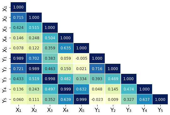
Figure 3: Pairwise correlations in the training examples. We denote the features in each example by $X_{j},$ and the single-targets in each multi-target by $Y_{j},$ where $j\in\{1,2,\dots,5\}$ is the number of superconducting qubits utilized in the benchmark task Roushan_2017 ; Neill_2018 ; Chiaro_2019 .

The boosting algorithm proceeds by reducing the multi-target regression task to $5$ independent single-target regression subtasks Borchani_2015 ; Waegeman_2019 . For the $jth$ single-target regression subtask, the $j$th single-target boosting algorithm induces the single-target regressor $\hat{h}_{j}$ on the $j$th slice of the training examples, where $j=\{1,2,\dots,5\}$ (see Eq. 11 in Methods). Subsequently, the boosting algorithm concatenates the single-target regressors into a multi-target regressor. Given a new example $X,$ the multi-target regressor predicts a $5$-dimensional real vector $\hat{Y}=\hat{h}(X).$

Gradient boosting prior knowledge – Boosting is an algorithmic paradigm for improving the performance of any given learning algorithm, interconnecting machine learning Powell_1987 ; Kearns_1988 ; Hastie_1990 ; Schapire_1990 ; Kearns_1994_3 ; Freund_1995 ; Freund_1997 ; Breiman_1997_1 ; Mason_1999 ; Schapire_2002 ; Chen_2016 ; Ke_2017 , statistics Tukey_1977 ; Friedman_2000 ; Friedman_2001 ; Friedman_2003 ; Hastie_2009 and signal processing Mallat_1993 ; Vincent_2002 ; Donoho_2012 through the study of additive expansions Hastie_1990 ; Friedman_2000 ; Friedman_2001 ; Hastie_2009 . Gradient boosting is a generic version of boosting, which is widely used in practice Friedman_2001 ; Friedman_2003 ; Hastie_2009 ; He_2014 ; Chen_2016 ; Ke_2017 , and the additive expansion is designed to finesse the curse of dimensionality and provide flexibility over linear models Hastie_1990 ; Friedman_2000 ; Friedman_2001 ; Friedman_2003 ; Hastie_2009 . Nonetheless, the standard form of gradient boosting does not allow for the direct incorporation of prior knowledge, which is essential in the benchmark task.

Here, we propose a modification of the standard additive expansion Friedman_2001 ; Friedman_2003 ; Hastie_2009 ; He_2014 ; Chen_2016 ; Ke_2017 for the $j$th single-target regression subtask

$$h_{j}(X;\{\alpha_{j},\theta_{j}\})=X_{j}+\sum_{k=1}^{K_{j}}\alpha_{j,k}b(X;\theta_{j,k})),$$ (2)

where the collection of expansion coefficients $\alpha_{j,k}$ and parameter sets $\theta_{j,k}$ is given by $\{\alpha_{j},\theta_{j}\}=\{\alpha_{j,1},\dots,\alpha_{j,K_{j}},\theta_{j,1},\dots,\theta_{j,K_{j}}\},$ and $K_{j}$ denotes the number of real-valued basis functions $b(X;\theta_{j,k})$ of the example $X$ (details in Methods). In the standard additive expansion, the first term is a constant offset value that does not depend upon the example, and it is usually determined by maximum likelihood estimation Hastie_1990 ; Friedman_2000 ; Friedman_2001 ; Friedman_2003 ; Hastie_2009 . In the work of Schapire et al, prior knowledge was incorporated into the Gödel prize winning AdaBoost algorithm by modifying the loss function for single-target classification tasks Schapire_2002 . In machine learning, the basis function is called a weak learner Kearns_1988 ; Schapire_1990 ; Kearns_1994_3 ; Freund_1995 ; Breiman_1997_1 ; Freund_1997 ; Schapire_2002 , and the predominant choice is a shallow decision tree Friedman_2001 ; Friedman_2003 ; Hastie_2009 ; He_2014 ; Chen_2016 ; Ke_2017 . Taking a reroughing viewpoint Tukey_1977 , Eq. 2 decomposes the $j$th single-target into a smooth term, i.e., the first term, and a noise term, i.e., the linear sum of basis functions. In the application, the classical control program Roushan_2017 ; Neill_2018 ; Chiaro_2019 generates the smooth term and the noise term adaptively models the relationships between the single-targets in Fig. 3 without overwhelming the prior knowledge (see Supplementary Information).

In practice, fitting an additive expansion by minimizing the data-based estimate of the $j$th single-target expected loss is usually infeasible Mallat_1993 ; Friedman_2000 ; Friedman_2001 ; Vincent_2002 ; Friedman_2003 ; Hastie_2009 ; Donoho_2012 (see Eq. 6 in Methods). Here, we employ a greedy stagewise algorithm to approximate this optimization problem, whereby the stagewise algorithm sequentially appends basis functions to the additive expansion without adjusting the previously learned expansion coefficients or parameter sets, as opposed to a stepwise algorithm Mallat_1993 ; Friedman_2000 ; Friedman_2001 ; Vincent_2002 ; Friedman_2003 ; Hastie_2009 ; Donoho_2012 (see Alg. 1 in Methods). As a result of modifying the standard additive expansion in Eq. 2, the learning framework directly incorporates prior knowledge into gradient boosting Friedman_2001 ; Friedman_2003 ; Hastie_2009 ; He_2014 ; Chen_2016 ; Ke_2017 by changing the initialization step (details in Methods). As an aside, this idea can be applied in compressed sensing by similarly changing the initialization step in matching pursuit and its extensions Mallat_1993 ; Vincent_2002 ; Donoho_2012 .

Inbuilt model selection – The greedy stagewise algorithm does not always improve performance over the smooth term. Hence, we introduce an augmented version with inbuilt model selection, which scores the incumbent smooth term and the candidate greedy stagewise algorithm with a modification of $k$-fold cross-validation (details in Methods). If the incumbent performs better or equally well, then the augmented version returns the smooth term as the induced single-target regressor. Otherwise, the augmented version calls the candidate (see Alg. 2 in Methods).

In Fig. 4, we illustrate the model selection step with an augmented learning curve for the single-target regression subtask $Y_{3}$ with training sizes varying between $23$ to $95$ ordered pairs.

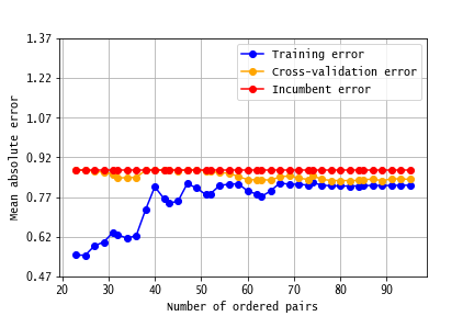
Figure 4: Augmented learning curve for the single-target $Y_{3}.$ We show the training, cross-validation, and incumbent errors for varying amounts of training examples in blue, orange, and red, respectively. As a consequence of the inbuilt model selection step, the cross-validation error is bounded from above by $0.87$ MHz. With $51,$ or more, ordered pairs the candidate greedy stagewise algorithm always outperforms the incumbent smooth term Roushan_2017 ; Neill_2018 ; Chiaro_2019 .

Here, the augmented learning curve shows the incumbent error (red) in addition to the training and cross-validation errors (blue and yellow) shown in a prototypical learning curve Hastie_2009 ; Sklearn_2011 ; Ng_2020 . The incumbent error bounds the cross-validation error from above. As the training size increases, the training error tends to increase, the cross-validation error tends to decrease, and both errors exhibit random fluctuations, which typically occur with less than $100$ ordered pairs Ng_2020 . When there are less than $51$ ordered pairs, the incumbent usually performs better, whereas the candidate always outperforms the incumbent with $51,$ or more, ordered pairs.

For the single-target regression subtasks $Y_{1},$ $Y_{2},$ and $Y_{5},$ the candidate always performs better, and in general the candidate always performs better with $60,$ or more, ordered pairs (see Supplementary Information). Thus, the boosting algorithm used the greedy stagewise algorithm in each single-target regression subtask in Fig. 2, where the boosting algorithm outperforms the baseline of expert human-level performance Roushan_2017 ; Neill_2018 ; Chiaro_2019 by over $20\%.$

Examining the prior knowledge – Data preprocessing can significantly impact generalization performance, especially if there is a shortage of training examples Erhan_2010 ; Sklearn_2011 . Here, we examine the classical control program Roushan_2017 ; Neill_2018 ; Chiaro_2019 as a data preprocessor for the downstream boosting algorithm, whereby the classical control program transforms $5$ qubit and $4$ coupler bias features from an instance of the spectroscopy protocol Roushan_2017 into an initial multi-target prediction (see Supplementary Information). Namely, we regard a collection of $5$ qubit and $4$ coupler bias features as an example, and we induce a fully-connected neural network Sklearn_2011 for each single-target. Next, we apply the SHAP framework to approximate each induced neural network with a simpler linear explanation model Lundberg_2017 (see Eq. 12 in Methods). The linear coefficients, known as SHAP values, allocate the importance of each feature for each single-target training data prediction Lundberg_2017 ; Molnar_2020 .

In Fig. 5, we acquire an overview of each feature’s importance and effect in the single-target regression subtask $Y_{1}$ Lundberg_2017 ; Molnar_2020 (see Eq. 13 in Methods; see Supplementary Information for additional SHAP summary plots).

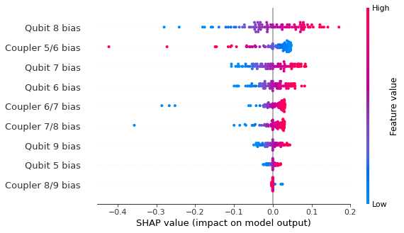
Figure 5: SHAP summary plot Lundberg_2017 for the single-target $Y_{1}.$ Using the collection of $9$ qubit and coupler bias features as an example, we induce a fully connected neural network Sklearn_2011 to predict $Y_{1}.$ The horizontal axis is centered at the average training example prediction, and the vertical axis ascendingly orders the features according to their importance. Each point is a SHAP value for a particular example, the coloring represents the bias value, and overlapping points are randomly jittered along the vertical axis to avoid collisions Lundberg_2017 ; Molnar_2020 .

The features are ascendingly ordered from bottom to top according to their importance, a point represents a SHAP value, and the coloring represents the bias value, e.g., a reddish point for the coupler $5/6$ bias feature illustrates strong coupling at the coupler between the $5$th and $6$th qubit sites. As can be clearly seen in Fig. 5, the qubit $8$ bias is the most important feature, which corresponds to an interior qubit site near the physical boundary of the linear chain. The coupler $5/6$ bias is the only coupler bias in the top $4$ features.

In comparison, the coupler $5/6$ bias is the most important feature in the single-target regression subtasks $Y_{3}$ and $Y_{4},$ and the coupler $8/9$ bias is the most important feature in the single-target regression subtasks $Y_{2}$ and $Y_{5}$ (see Supplementary Information). The former feature corresponds to a coupler near the experimentally imposed boundary of the linear chain, and the latter feature corresponds to a coupler near the physical boundary of the linear chain. Whereas the qubit biases, which correspond to interior qubit sites, are $3$ out of the $4$ most important features in the single-target regression subtask $Y_{1},$ the only other single-target regression subtask with a qubit bias in the top $4$ features is $Y_{2}.$

This feature dependence merits some discussion. As each instance of the spectroscopy protocol Roushan_2017 ascendingly orders the eigenenergies, one might expect that on average over all runs the feature dependence would be qualitatively the same for each single-target. Indeed, under independent and identically distributed sampling of the input parameters we would expect the data to exhibit a symmetry under permutation among the local bias and coupling parameters in Eq. 1. In line with this intuition, we observe a noticeably marked dependence on the coupler bias features closest to the physical boundaries for all single-targets. However, more generally, the permutation symmetry is broken in the benchmark dataset, not least because the model consists of few sites and is patently not well approximated by closed boundary conditions. Some of the individual single-targets, for instance, have a stronger dependence on specific on-site biases than others. This suggest that different sites correlate more strongly with larger or smaller eigenenergies. An example is the aforementioned strong dependence of the most negative eigenenergy $Y1$ on the on-site bias at site $8$. We attribute this to the geometry of the physical configuration and note that this asymmetric feature dependence is already present in the initial multi-target predictions generated by the data preprocessor.

Discussion

While entirely data-driven approaches are successful in machine learning applications with an abundance of data, these machine learning methods break down in scenarios with a shortage of data. Overcoming this obstacle requires some resource that compensates for the lack of data Schapire_2002 . In quantum device calibration applications, data accumulation is low Roushan_2017 , but there is an analytical model of the domain based upon prior scientific discoveries. Our result demonstrates that a machine learner can refine and enhance such discoveries with a minuscule amount of real experimental data. Using this approach, our learning system surpassed its scientific contemporaries Roushan_2017 ; Neill_2018 ; Chiaro_2019 by over $20\%$ on the superconducting quantum device calibration task, thereby providing a pathway for the successful interface of artificial intelligence and physics. Moreover, we have demonstrated the robustness of our approach by incorporating inbuilt model selection and we have established a diagnostic method to examine the underlying scientific model with SHAP learning techniques Lundberg_2017 ; Molnar_2020 .

Although we have focused on a quantum device calibration application, the presented machine learning approach can have significant impact further afield. We have introduced an additive expansion in Eq. 2 that is a modification of a model at the heart of several function approximation methods in engineering Powell_1987 , machine learning Powell_1987 ; Schapire_1990 ; Freund_1995 ; Freund_1997 ; Breiman_1997_1 ; Mason_1999 ; Chen_2016 ; Ke_2017 , statistics Tukey_1977 ; Hastie_1990 ; Friedman_2000 ; Friedman_2001 ; Friedman_2003 ; Hastie_2009 and signal processing Mallat_1993 ; Vincent_2002 ; Donoho_2012 . Gradient boosting is one of the most popular learning algorithms in data science and machine learning competitions Chen_2016 ; Ke_2017 , and also in real-world production pipelines He_2014 . Our approach enables it to take advantage of prior knowledge, especially when data is scarce. Other potential applications include compressed sensing, where prior knowledge about sparsity has resulted in an advantage over the Nyquist-Shannon sampling theorem Mallat_1993 ; Vincent_2002 ; Donoho_2012 . Indeed, physical manifestations of Occam’s razor, symmetry and complexity have already significantly influenced the development of learning and prediction Shalizi_2001 ; Gu_2012 ; Lin_2017 ; Udrescu_2020 – and thus a systematic approach to incorporating prior scientific knowledge into a machine learner provides a natural advancement of the mutualistic relationship between human researchers and artificial intelligence.

Methods

Multi-target regression background – In the setting of our learning framework, let $\mathcal{X}$ be the domain, where we refer to points in $\mathcal{X}$ as examples. Let $\mathcal{Y}\subseteq\mathbb{R}^{n}$ be the target space of multi-target observations, where we refer to vectors in $\mathcal{Y}$ as multi-targets and to components of vectors as single-targets. We refer to an ordered pair in the product of the domain and the target space $(X,Y)\in\mathcal{X}\times\mathcal{Y}$ as a labeled example. Moreover, we are given a finite sequence of labeled examples

$$S=\{(X^{(i)},Y^{(i)})\}_{i=1}^{m}\in(\mathcal{X}\times\mathcal{Y})^{m},$$ (3)

which is supposed random so that there is an unknown probability distribution on $\mathcal{X}\times\mathcal{Y}$ Haussler_1992 ; Kearns_1994_1 ; Kearns_1994_2 .

We wish to find some simple pattern in the labeled examples, namely a multi-target regressor $h:\mathcal{X}\to\mathcal{Y}.$ However, there may be no functional relationship between the domain and the target space in this agnostic setting Kearns_1994_1 ; Kearns_1994_2 . In order to measure the predictive prowess of a multi-target regressor, we introduce the decision theoretic concept of a loss function Haussler_1992 ; Kearns_1994_1 ; Kearns_1994_2 ; Friedman_2001 ; Friedman_2003 ; Hastie_2009 , where we denote a non-negative multi-target loss function by $\ell:\mathcal{Y}\times\mathcal{Y}\to\mathbb{R}_{\geq 0}.$ Given a labeled example $(X,Y)\in\mathcal{X}\times\mathcal{Y},$ the loss of some multi-target regressor $h$ on the labeled example is denoted by $\ell(Y,h(X)).$ The multi-target loss function measures the magnitude of error in predicting $h(X),$ when the multi-target is $Y.$

Here, we study loss functions that are decomposable over the targets, which provides a joint target view Borchani_2015 ; Waegeman_2019 . Let $\mathcal{Y}_{j}\subseteq\mathbb{R}$ be the single-target space of the $j$th single-target observations. We denote a single-target regressor by $h_{j}:\mathcal{X}\to\mathcal{Y}_{j}.$ We denote a nonnegative single-target loss function by $\ell_{j}:\mathcal{Y}_{j}\times\mathcal{Y}_{j}\to\mathbb{R}_{\geq 0}.$ Given a labeled example in the product of the domain and the single-target space $(X,Y_{j})\in\mathcal{X}\times\mathcal{Y}_{j},$ the loss of some single-target regressor $h_{j}$ on the labeled example is denoted $\ell_{j}(Y_{j},h_{j}(X)).$ The single-target loss function measures the magnitude of error in predicting $h_{j}(X),$ when the single-target is $Y_{j}.$ We define a loss function that is decomposable over the targets by

$$\ell(Y,h(X))=\sum_{j=1}^{n}\ell_{j}(Y_{j},h_{j}(X)),$$ (4)

in accord with Borchani_2015 ; Waegeman_2019 . In the application, we study the absolute error loss function, which is decomposable over the targets. Namely,

$$\begin{split}\ell(Y,h(X))&=||Y-h(X)||_{1}\\ &=\sum_{j=1}^{n}|Y_{j}-h_{j}(X)|\\ &=\sum_{j=1}^{n}\ell_{j}(Y_{j},h_{j}(X)),\end{split}$$ (5)

where $||\cdot||_{p}$ denotes the $\mbox{L}^{p}$ norm. Using the joint view, the multi-target regression task reduces to $n$ independent single-target regression subtasks

$$\mathbb{E}_{X,Y}[\ell(Y,h(X))] =\mathbb{E}_{X,Y}[\sum_{j=1}^{n}\ell_{j}(Y_{j},h_{j}(X))]$$

$$=\sum_{j=1}^{n}\mathbb{E}_{X,Y_{j}}[\ell_{j}(Y_{j},h_{j}(X))],$$ (6)

where the first line follows from the choice of a loss function that is decomposable over the targets, and the second line follows from linearity Borchani_2015 ; Waegeman_2019 . In this case, the optimal $j$th single-target regressor is the one that minimizes the $j$th single-target expected loss

$$h^{*}_{j}=\operatorname*{\arg\!\min}_{h_{j}}\mathbb{E}_{X,Y_{j}}[\ell_{j}(Y_{j},h_{j}(X))].$$ (7)

Under the distribution-free setting, the $j$th single-target expected loss is not available Haussler_1992 ; Kearns_1994_1 ; Kearns_1994_2 ; Friedman_2001 ; Friedman_2003 ; Hastie_2009 . Consequently, we split Eq. 3 into training, validation, and test data, if there is sufficient data for an explicit validation stage. Otherwise, we forgo the validation split. Here, we focus on the case of splitting Eq. 3 into $m_{train}$ and $m_{test}$ ordered pairs for training and test data, respectively, as there is a shortage of labeled examples in the application. Moreover, we isolate the test data from the training data, whereby training data is recyclable and test data is single-use. Using the test data, we approximate the $j$th single-target expected loss with the mean absolute error

$$\frac{1}{m_{test}}\sum_{i=1}^{m_{test}}|Y^{(i)}_{j}-h_{j}(X^{(i)})|.$$ (8)

Then, we approximate the expected loss with the average mean absolute error

$$\frac{1}{n}\sum_{j=1}^{n}\frac{1}{m_{test}}\sum_{i=1}^{m_{test}}|Y^{(i)}_{j}-h_{j}(X^{(i)})|,$$ (9)

and we refer to this error as the benchmark error in Fig. 2.

Two-step stacking framework – In the learning framework, let $\mathcal{X}\subseteq\mathbb{R}^{n}$ be the domain of initial multi-target predictions generated by a base regressor. We assume the availability of these predictions as well as the associated multi-target observations. In this way, the learning framework can be applied in tandem with scientific models (see the Supplementary Information for a brief review of the traditional two-step stacking approach).

In the first step, we wrangle the labeled examples Eq. 3, and we represent them with an $m\times 2n$ design matrix

$$\begin{pmatrix}\rule[2.15277pt]{35.00005pt}{0.4pt}X^{(1)}\rule[2.15277pt]{35.00005pt}{0.4pt}&\vline&\rule[2.15277pt]{35.00005pt}{0.4pt}Y^{(1)}\rule[2.15277pt]{35.00005pt}{0.4pt}\\ \rule[2.15277pt]{35.00005pt}{0.4pt}X^{(2)}\rule[2.15277pt]{35.00005pt}{0.4pt}&\vline&\rule[2.15277pt]{35.00005pt}{0.4pt}Y^{(2)}\rule[2.15277pt]{35.00005pt}{0.4pt}\\ \vdots&\vline&\vdots\\ \rule[2.15277pt]{35.00005pt}{0.4pt}X^{(m)}\rule[2.15277pt]{35.00005pt}{0.4pt}&\vline&\rule[2.15277pt]{35.00005pt}{0.4pt}Y^{(m)}\rule[2.15277pt]{35.00005pt}{0.4pt}\\ \end{pmatrix},$$ (10)

where $m$ denotes the number of multi-targets and $n$ denotes the number of single-targets. Next, we split Eq. 10 into $m_{train}$ and $m_{test}$ rows for training and test data, respectively. In the second step, the boosting algorithm receives the training data, which has shape $m_{train}\times 2n,$ and we request a multi-target regressor as output. In the $j$th single-target regression subtask, the boosting algorithm slices the $j$th single-target from the training data

$$\begin{pmatrix}\rule[2.15277pt]{35.00005pt}{0.4pt}X^{(1)}\rule[2.15277pt]{35.00005pt}{0.4pt}&\vline&Y_{j}^{(1)}\\ \rule[2.15277pt]{35.00005pt}{0.4pt}X^{(2)}\rule[2.15277pt]{35.00005pt}{0.4pt}&\vline&Y_{j}^{(2)}\\ \vdots&\vline&\vdots\\ \rule[2.15277pt]{25.00003pt}{0.4pt}X^{(m_{train})}\rule[2.15277pt]{25.00003pt}{0.4pt}&\vline&Y_{j}^{(m_{train})}\\ \end{pmatrix},$$ (11)

where the matrix has shape $m_{train}\times(n+1).$ Next, the single-target boosting algorithm detailed in Alg. 2 induces the $j$th single-target regressor $\hat{h}_{j}$ on Eq. 11. After completion of each single-target regression subtask, the boosting algorithm concatenates the induced single-target regressors into the multi-target regressor $\hat{h}=(\hat{h}_{1},\hat{h}_{2},\dots,\hat{h}_{n})^{T}$. Given a new example $X\in\mathcal{X},$ the multi-target regressor predicts an $n$-dimensional real vector $\hat{Y}=\hat{h}(X)$ (see Fig. 2).

Model selection – As the test data is single-use, we need to simultaneously select the best performing single-target boosting algorithm detailed in Alg. 1 for the $j$th single-target regression subtask and estimate the $j$th mean absolute error Eq. 8, where $j\in\{1,2,\dots,n\}.$ Moreover, we need to ensure that the selected $j$th single-target boosting algorithm is able to choose the smooth term, if the noise term in Eq. 2 degrades performance (see Fig. 4). For this objective, we review nested cross-validation Hastie_2009 ; Cawley_2010 ; Sklearn_2011 , and we describe the modification of $k$-fold cross-validation utilized in Alg. 2, which is similar to learning algorithms with inbuilt cross-validation Sklearn_2011 .

In Fig. 6, we illustrate $k$-fold cross-validation, e.g., $k=5,$ which is a precursor for nested cross-validation Hastie_2009 ; Cawley_2010 ; Sklearn_2011 and the inbuilt model selection step in Alg. 2. The method begins by randomly partitioning Eq. 11 into $k$ non-overlapping folds, and $k$ is typically a natural number between $5$ and $10,$ inclusive.

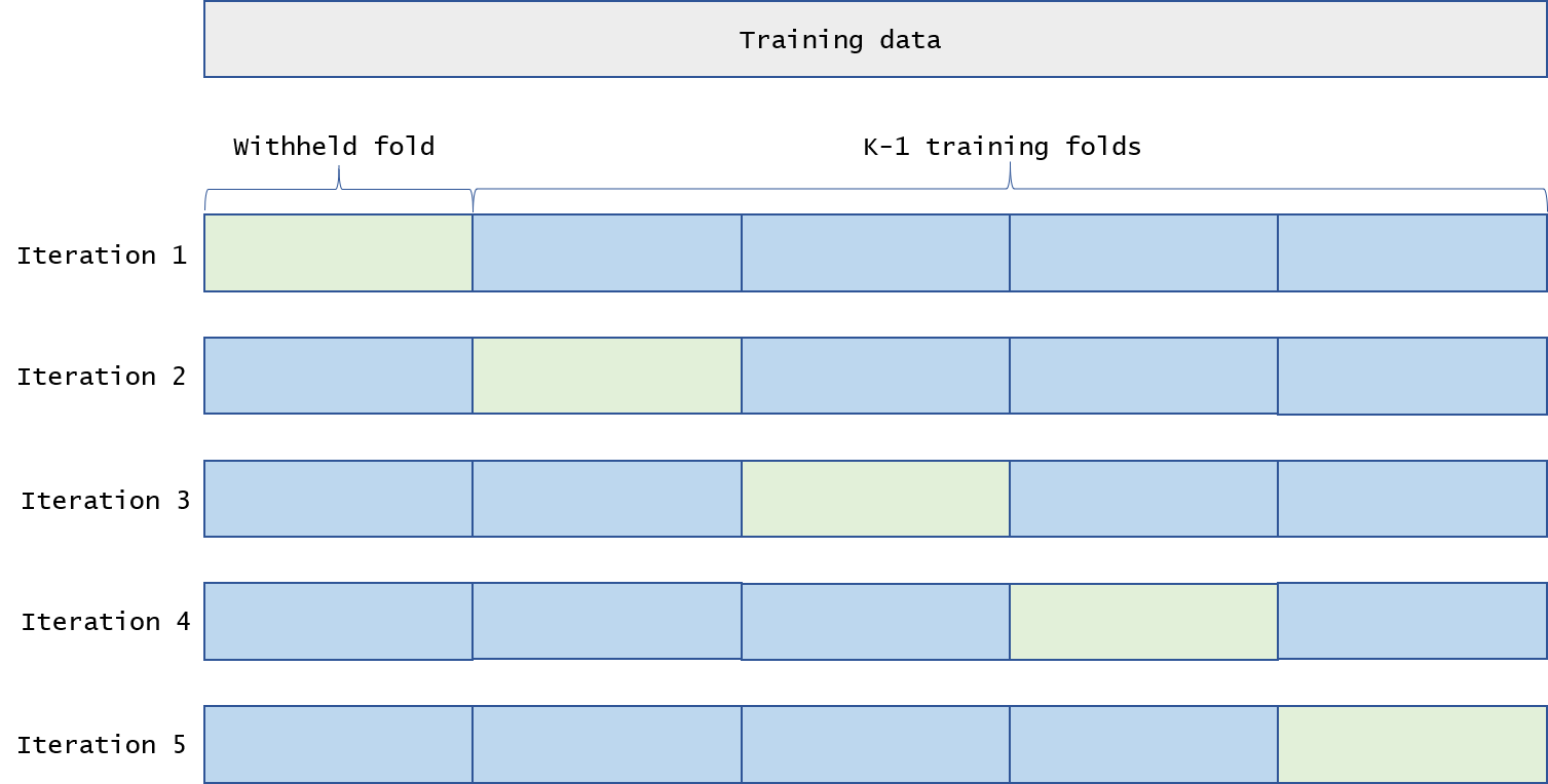
Figure 6: $k$-fold cross-validation. We represent the training data as a light grey rectangle, and we illustrate $5$-fold cross-validation on the training data. In each iteration, the withheld fold is colored light green and the $4$ training folds are colored light blue. We note that each of the withheld folds is used exactly once as the validation data.

Next, we repeat the following two steps $k$ times with each of the withheld folds used exactly once as the validation data:

• Of the $k$ folds, we withhold one for validation. A single-target boosting algorithm receives the remaining $k-1$ folds as training data, and we request a single-target regressor as output.

• We evaluate the induced single-target regressor on the withheld fold from the previous step by computing the average loss of the single-target regressor.

Then, we average the $k$ results from the second step, and we refer to this average as cross-validation error. This completes a single loop of the $k$-fold cross-validation method. In best practices of machine learning, this method is preferred over leave-one-out cross-validation, wherein $k=m_{train}$ Hastie_2009 ; Cawley_2010 ; Sklearn_2011 .

In nested cross-validation, the estimation method utilizes an outer loop of $k$ non-overlapping folds and an inner loop of $l$ non-overlapping folds. The outer loop is utilized to estimate the $j$th mean absolute error Eq. 8 and the inner loop is utilized to select the (hyper)parameters in Alg. 1, such as the choice of basis function or value of $K_{j}$ in Eq. 2. The method begins by randomly partitioning Eq. 11 into $k$ non-overlapping folds. Next, we repeat the following two steps $k$ times with each of the withheld folds in the outer loop used exactly once as the validation data:

• Of the $k$ folds, we withhold a fold for validation. In the inner loop, we apply $l$-fold cross-validation to the remaining $k-1$ folds for multiple single-target boosting algorithms with differing (hyper)parameters. After completing the inner loop, we select the best performing single-target boosting algorithm based on the minimum inner loop cross-validation error.

• The selected single-target boosting algorithm receives the $k-1$ folds from the previous step as training data, and we request a single-target regressor as output. We evaluate the induced single-target regressor on the withheld fold from the previous step by computing the average loss of the single-target regressor.

Then, we average the $k$ results from the second step, and we use this average to approximate the $j$th mean absolute error Eq. 8. In practice, we usually execute nested cross-validation within an exhaustive hyperparameter search tool, such as $GridSearchCV$ by scikit-learn Sklearn_2011 (see Supplementary Information for implementation details).

After completing nested cross-validation, we repeat the second step in the learning framework. In the $j$th single-target regression subtask, Alg. 2 utilizes Eq. 11 in a modified $k$-fold cross-validation procedure to select either the incumbent smooth term from the base regressor or the candidate additive expansion Eq. 2 as the induced single-target regressor. This entails modifying the second step in the aforedescribed $k$-fold cross-validation method, namely

• We independently evaluate the smooth term and the induced single-target regressor on the withheld fold from the previous step by computing the average loss of the smooth term and the single-target regressor. We note that the smooth term always predicts the $j$th feature, given an example from the withheld fold.

Then, we independently average their $k$ results, and we refer to these averages as the incumbent error and the cross-validation error, respectively. The inbuilt model selection step in Alg. 2 selects the better algorithm based on the minimum error. Subsequently, the boosting algorithm completes each single-target regression subtask, and the boosting algorithm returns the induced multi-target regressor for evaluation on the test data.

Single-target gradient boosting – For the $j$th single-target regression subtask, the single-target boosting algorithm Alg. 1 takes as input training examples Eq. 11, number of iterations $K_{j},$ single-target loss functions $\{\ell_{j},\tilde{\ell}_{j}\},$ and basis function $b$ characterized by parameter set $\theta.$

Input : training examples

number of iterations $K_{j}$

single-target loss functions $\{\ell_{j},\tilde{\ell}_{j}\}$

basis function $b$ characterized by parameter set $\theta$

Initialize: $h_{j,0}(X)=X_{j}$ for each example

for $k=1$ to $K_{j}$ do

1.  

   for $i=1$ to $m_{train}$ do

             Compute pseudo-residuals

               $r^{(i)}_{j,k}=-\frac{\partial\ell_{j}(Y_{j}^{(i)},h_{j}(X^{(i)}))}{\partial h_{j}(X^{(i)})}\bigg{|}_{h_{j}(X^{(i)})=h_{j,k-1}(X^{(i)})}$

       end for

Induce a basis function on $\{X^{(i)},r_{j,k}^{(i)}\}_{i=1}^{m_{train}}$ to learn the parameter set $\theta_{j,k}$ (c)   Solve the one-dimensional optimization problem to learn the expansion coefficient

$\alpha_{j,k}=\operatorname*{\arg\!\min}_{\alpha}\sum_{i=1}^{m_{train}}\tilde{\ell}_{j}(Y^{(i)}_{j},h_{j,k-1}(X^{(i)})+\alpha b(X^{(i)};\theta_{j,k}))$

 

Sequentially append the induced basis function to the additive expansion

       $h_{j,k}(X)=h_{j,k-1}(X)+\alpha_{j,k}b(X;\theta_{j,k})$

end for

Output : Single-target regressor $\hat{h}_{j}=h_{j,K_{j}}$

Algorithm 1 $BaseBoost$

For instance, the parameter set would encode the split features, split locations, and the terminal node means of the individual trees, if the choice of basis function were a shallow decision tree; see for example Friedman_2001 ; Friedman_2003 ; Hastie_2009 ; Chen_2016 ; Ke_2017 . In the application, we choose a stacking regressor Wolpert_1992 ; Breiman_1996 ; Sklearn_2011 as the basis function, which is a two layer ensemble of single-target regressors (see Supplementary Information).

In Alg. 1, the first line initializes to the smooth term for each example in Eq. 11. In the for loop, line (a) computes the pseudo-residuals with single-target loss function $\ell_{j},$ whereby the term pseudo-residual emanates from the term residual in least squares fitting and reroughing Tukey_1977 ; Friedman_2001 ; Friedman_2003 ; Hastie_2009 . Line (b) enables the boosting algorithm to work for any given single-target learning algorithm Friedman_2001 ; Friedman_2003 ; Hastie_2009 , whereby the labels are the pseudo-residuals from line (a). Line (c) computes the one-dimensional line search with single-target loss function $\tilde{\ell}_{j}.$ Line (d) sequentially appends the basis function to the additive expansion. The output is the induced single-target regressor $\hat{h}_{j}$.

In the application, we modify line (c) in Alg. 1 to include $\mbox{L}^{1}$ regularization (see the Supplementary Information). In relation to previous work, the initialization step in Alg. 1 depends upon the examples, whereas the standard form of gradient boosting initializes to the optimal constant model: $\operatorname*{\arg\!\min}_{c}\sum_{i=1}^{m_{train}}\ell_{j}(Y_{j}^{(i)},c);$ see references Friedman_2001 ; Friedman_2003 ; Hastie_2009 . In matching pursuit and its extensions, the greedy stagewise algorithms initialize to the zero vector, and they sequentially transform the signal into a negligible residual; see references Mallat_1993 ; Vincent_2002 ; Donoho_2012 for the algorithmic body differences and further details.

For the $j$th single-target regression subtask, the augmented version of the single-target boosting algorithm Alg. 2 takes as input training examples Eq. 11, number of iterations $K_{j},$ single-target loss functions $\{\ell_{j},\tilde{\ell}_{j}\},$ basis function $b$ characterized by parameter set $\theta,$ number of cross-validation folds $k,$ and $k$-fold cross-validation single-target loss function.

Input : training examples

number of iterations $K_{j}$

single-target loss functions $\{\ell_{j},\tilde{\ell}_{j}\}$

basis function $b$ characterized by parameter set $\theta$

number of cross-validation folds $k$

$k$-fold cross-validation single-target loss function

Model selection: Perform modified $k$-fold cross-validation for the incumbent smooth term and the candidate $BaseBoost.$ If the incumbent error is less than or equal to the cross-validation error, then break $\hat{h}_{j}(X)=X_{j}.$ Otherwise, call $BaseBoost.$

Output : Single-target regressor $\hat{h}_{j}$

Algorithm 2 $BaseBoostCV$

The inbuilt model selection step in Alg. 2 selects the incumbent smooth term as the induced single-target regressor, if the incumbent error is less than or equal to the cross-validation error, otherwise Alg. 2 calls Alg. 1 ($k$-fold cross-validation details in previous section). The output is the induced single-target regressor $\hat{h}_{j}$.

Explainable machine learning – In machine learning competitions and products, complex models, such as ensemble and deep learning models, are omnipresent. Understanding why these models make certain predictions is the focus of explainable machine learning Lundberg_2017 ; Molnar_2020 . The SHAP framework unifies several approaches in explainable machine learning to replicate individual predictions generated by a single-target regressor with a simpler linear explanation model whose coefficients measure feature importance Lundberg_2017 . In the work of S̆trumbelj and Kononenko, these coefficients, known as SHAP values Lundberg_2017 , were shown to be equivalent to the Shapley value in cooperative game theory Strumbelj_2014 . The explanation model is defined as a linear function of binary variables

$$g(z^{\prime})=\phi_{0}+\sum_{k=1}^{M}\phi_{k}z^{\prime}_{k}$$ (12)

where $z^{\prime}\in\{0,1\}^{M}$ is a set of binary variables, $M$ is the number of features under consideration, and $\phi_{k}$ is a real-valued feature attribution, known as a SHAP value, for the $k$th feature. As the computation of Shapley values has an exponential time complexity Strumbelj_2014 , the SHAP software approximates the coefficients with insights from additive feature attribution methods; see Lundberg_2017 .

In the application, we utilize the model-agnostic approximation method, known as Kernel SHAP, to compute the SHAP values Lundberg_2017 . This enables us to ascertain a simpler explanation model to approximate each training data prediction generated by the induced fully-connected neural networks Sklearn_2011 , where $M=9$ in Eq. 12 for the control voltage features (see the Supplementary Information). The importance $I$ of each feature is defined as the sum of absolute SHAP values

$$I_{k}=\sum_{i=1}^{m_{train}}|\phi_{k}^{(i)}|,$$ (13)

which enables an ordering to be defined. The features are sorted in ascending order from bottom to top in each summary plot Lundberg_2017 ; Molnar_2020 .

Data Availability

All data, relevant to the information and figures presented in this manuscript, are available upon reasonable request.

Author Contributions

A.W. designed the learning approach, implemented the learning system, and performed the data analysis. All authors contributed to the interpretation of the data and to writing the manuscript.

in 1,…,8 See pages \x, of supplementary

References

- [1] David Hume. A Treatise of Human Nature. Clarendon Press, 1739.
- [2] David Haussler. Quantifying inductive bias: AI learning algorithms and Valiant’s learning framework. Artificial Intelligence, 36:177–221, 1988.
- [3] Tom Mitchell. The need for biases in learning generalisation. In Jude Shavlik and Thomas Dietterich, editors, Readings in Machine Learning. Morgan Kaufmann, 1991.
- [4] David Wolpert and William Macready. No free lunch theorems for optimization. IEEE Transactions on Evolutionary Computation, 1(1), 1997.
- [5] Rich Caruana. Multitask learning. Machine Learning, 28:41–75, 1997.
- [6] Jonathan Baxter. A model of inductive bias learning. Journal of Artificial Intelligence Research, 12:149–198, 2000.
- [7] Steven Brunton, Joshua Proctor, and José Nathan Kutz. Discovering governing equations from data by sparse identification of nonlinear dynamical systems. Proceedings of the National Academy of Sciences of the United States of America, 113(15):3932–3937, 2016.
- [8] Pedram Roushan et al. Spectroscopic signatures of localization with interacting photons in superconducting qubits. Science, 358:1175–1179, 2017.
- [9] Keith Butler et al. Machine learning for molecular and materials science. Nature, 559:547–555, 2018.
- [10] Charles Neill et al. A blueprint for demonstrating quantum supremacy with superconducting qubits. Science, 360:195–199, 2018.
- [11] Benjamin Chiaro et al. Growth and preservation of entanglement in a many-body localized system. arXiv:1910.06024, 2019.
- [12] Michael Schmidt and Hod Lipson. Distilling free-form natural laws from experimental data. Science, 324:81–85, 2009.
- [13] Juan Carrasquilla and Roger Melko. Machine learning phases of matter. Nature Physics, 13:431–434, 2017.
- [14] Alexey Melnikov et al. Active learning machine learns to create new quantum experiments. Proceedings of the National Academy of Sciences of the United States of America, 115(6):1221–1226, 2018.
- [15] Maciej Koch-Janusz and Zohar Ringel. Mutual information, neural networks and the renormalization group. Nature Physics, 14:578–582, 2018.
- [16] Giacomo Torlai et al. Neural-network quantum state tomography. Nature Physics, 14:447–450, 2018.
- [17] Tailin Wu and Max Tegmark. Toward an artificial intelligence physicist for unsupervised learning. Physical Review E, 100:033311, 2019.
- [18] Raban Iten et al. Discovering physical concepts with neural networks. Physical Review Letters, 124:010508, 2020.
- [19] Sebastian Wetzel et al. Discovering symmetry invariants and conserved quantities by interpreting siamese neural networks. arXiv:2003.04299, 2020.
- [20] Hanen Borchani et al. A survey on multi-output regression. Wiley Interdisciplinary Reviews: Data Mining and Knowledge Discovery, 2015.
- [21] Willem Waegeman, Krzysztof Dembczyński, and Eyke Hüllermeier. Multi-target prediction: A unifying view on problems and methods. Data Mining and Knowledge Discovery, 33:293–324, 2019.
- [22] Fabian Pedregosa et al. Scikit-learn: machine learning in python. Journal of Machine Learning Research, 12:2825–2830, 2011.
- [23] Alvaro Pascual-Leone et al. The plastic human brain cortex. Annual Review of Neuroscience, 28:377–401, 2005.
- [24] Yu Chen et al. Qubit architecture with high coherence and fast tunable coupling. Physical Review Letters, 113:220502, 2014.
- [25] Ehsan Zahedinejad, Joydip Ghosh, and Barry Sanders. Designing high-fidelity single-shot three-qubit gates: a machine-learning approach. Physical Review Applied, 6:054005, 2016.
- [26] Henry Lin, Max Tegmark, and David Rolnick. Why does deep and cheap learning work so well? Journal of Statistical Physics, 168(6):1223–1247, 2017.
- [27] Jacob Biamonte et al. Quantum machine learning. Nature, 549:195–202, 2017.
- [28] Vedran Dunjko and Hans Briegel. Machine Learning & Artificial Intelligence in the Quantum Domain: A Review of Recent Progress. Reports on Progress in Physics, 81(7), 2018.
- [29] Giuseppe Carleo et al. Machine learning and the physical sciences. Reviews of Modern Physics, 91:045002, 2019.
- [30] Pankaj Mehta et al. A high-bias, low-variance introduction to Machine Learning for physicists. Physics Reports, 810:1–124, 2019.
- [31] Silviu-Marian Udrescu and Max Tegmark. AI Feynman: A physics-inspired method for symbolic regression. Science Advances, 6(16), 2020.
- [32] Scott Lundberg and Su-In Lee. A unified approach to interpreting model predictions. In Advances in Neural Information Processing Systems 30, pages 4765–4774. Curran Associates, Inc., 2017.
- [33] Christoph Molnar. Interpretable machine learning: a guide for making black box models explainable. christophm.github.io/interpretable-ml-book, 2020.
- [34] Norbert Linke et al. Experimental comparison of two quantum computing architectures. Proceedings of the National Academy of Sciences of the United States of America, 114(13):3305–3310, 2017.
- [35] Julian Kelly et al. Physical qubit calibration on a directed acyclic graph. arXiv:1803.03226, 2018.
- [36] David Wolpert. Stacked generalization. Neural Networks, 5:241–259, 1992.
- [37] Leo Breiman. Stacked regressions. Machine Learning, 24:49–64, 1996.
- [38] Leo Breiman and Jerome Friedman. Predicting multivariate responses in multiple linear regression. Royal Statistical Society Series B, 59:3–54, 1997.
- [39] Dumitru Erhan et al. Why does unsupervised pre-training help deep learning? Journal of Machine Learning Research, 11:625–660, 2010.
- [40] David Haussler. Decision theoretic generalizations of the PAC model for neural net and other learning applications. Information and Computation, 100:78–150, 1992.
- [41] Michael Kearns and Robert Schapire. Efficient distribution-free learning of probabilistic concepts. Journal of Computer and Systems Science, 48:464–497, 1994.
- [42] Michael Kearns, Robert Schapire, and Linda Sellie. Toward efficient agnostic learning. Machine Learning, 17:115–141, 1994.
- [43] Jerome Friedman. Greedy function approximation: A gradient boosting machine. Annals of Statistics, 29(5):1189–1232, 2001.
- [44] Jerome Friedman and Bogdan Popescu. Importance sampled learning ensembles. Technical report, Stanford University, Department of Statistics, 2003.
- [45] Trevor Hastie, Robert Tibshirani, and Jerome Friedman. The Elements of Statistical Learning. Springer, 2009.
- [46] Andrew Ng. Machine learning yearning. deeplearning.ai project, 2020.
- [47] Michael Powell. Radial basis functions for multivariable interpolation: a review. In Algorithms for Approximation. Clarendon Press, 1987.
- [48] Michael Kearns and Leslie Valiant. Learning boolean formulae or finite automata is as hard as factoring. Technical Report TR-14-88, Harvard University Aiken Computation Laboratory, 1988.
- [49] Trevor Hastie and Robert Tibshirani. Generalized Additive Models. Chapman and Hall, London, 1990.
- [50] Robert Schapire. The strength of weak learnability. Machine Learning, 5:197–227, 1990.
- [51] Michael Kearns and Leslie Valiant. Cryptographic limitations on learning boolean formulae and finite automata. Journal of the Association for Computing Machinery, 41:67–95, 1994.
- [52] Yoav Freund. Boosting a weak learning algorithm by majority. Information and Computation, 121:256–285, 1995.
- [53] Yoav Freund and Robert Schapire. A decision-theoretic generalization of on-line learning and an application to boosting. Journal of Computer and System Sciences, 55:119–139, 1997.
- [54] Leo Breiman. Arcing the edge. Technical report, Stanford University, Department of Statistics, 1997.
- [55] Llew Mason et al. Boosting algorithms as gradient descent. In NIPS: Proceedings of the th International Conference on Neural Information Processing, pages 512––518, 1999.
- [56] Robert Schapire et al. Incorporating prior knowledge into boosting. In ICML’02: Proceedings of the Nineteenth International Conference on Machine Learning, pages 538–545, 2002.
- [57] Tianqi Chen and Carlos Guestrin. XGBoost: a scalable tree boosting system. In KDD’16: Proceedings of the nd ACM SIGKDD International Conference on Knowledge Discovery and Data Mining, pages 785–794, 2016.
- [58] Guolin ke et al. LightGBM: a highly efficient gradient boosting decision tree. In Advances in Neural Information Processing Systems 30, pages 3149–3157. Curran Associates, Inc., 2017.
- [59] John Tukey. Exploratory Data Analysis. Addison-Wesley, 1977.
- [60] Jerome Friedman, Trevor Hastie, and Robert Tibshirani. Additive logistic regression: A statistical view of boosting. The Annals of Statistics, 28(2):337–407, 2000.
- [61] Stéphane Mallat and Zhifeng Zhang. Matching pursuits with time-frequency dictionaries. IEEE Transactions on Signal Processing, 41(12):3397–3415, 1993.
- [62] Pascal Vincent and Yoshua Bengio. Kernel matching pursuit. Machine Learning, 48:165–187, 2002.
- [63] David Donoho et al. Sparse solution of underdetermined systems of linear equations by stagewise orthogonal matching pursuit. IEEE Transactions on Information Theory, 58(2):1094–1121, 2012.
- [64] Xinran He et al. Practical lessons from predicting clicks on ads at facebook. In ADKDD’14: Proceedings of the Eighth International Workshop on Data Mining for Online Advertising, 2014.
- [65] Cosma Shalizi and James Crutchfield. Computational mechanics: Pattern and prediction, structure and simplicity. Journal of Statistical Physics, 104(3-4):817–879, 2001.
- [66] Mile Gu et al. Quantum mechanics can reduce the complexity of classical models. Nature communications, 3(1):1–5, 2012.
- [67] Gavin Cawley and Nicola Talbot. On over-fitting in model selection and subsequent selection bias in performance evaluation. Journal of Machine Learning Research, 11:2079–2107, 2010.
- [68] Erik S̆trumbelj and Igor Kononenko. Explaining prediction models and individual predictions with feature contributions. Knowledge and Information Systems, 41:647–665, 2014.