AMYTISS: Parallelized Automated Controller Synthesis for Large-Scale Stochastic Systems

Abstract.

In this paper, we propose a software tool, called AMYTISS, implemented in C++/OpenCL, for designing correct-by-construction controllers for large-scale discrete-time stochastic systems. This tool is employed to (i) build finite Markov decision processes (MDPs) as finite abstractions of given original systems, and (ii) synthesize controllers for the constructed finite MDPs satisfying bounded-time high-level properties including safety, reachability and reach-avoid specifications. In AMYTISS, scalable parallel algorithms are designed such that they support the parallel execution within CPUs, GPUs and hardware accelerators (HWAs). Unlike all existing tools for stochastic systems, AMYTISS can utilize high-performance computing (HPC) platforms and cloud-computing services to mitigate the effects of the state-explosion problem, which is always present in analyzing large-scale stochastic systems. We benchmark AMYTISS against the most recent tools in the literature using several physical case studies including robot examples, room temperature and road traffic networks. We also apply our algorithms to a $3$-dimensional autonomous vehicle and $7$-dimensional nonlinear model of a BMW $320$i car by synthesizing an autonomous parking controller.

1. Introduction

1.1. Motivations

Large-scale stochastic systems are an important modeling framework to describe many real-life safety-critical systems such as power grids, traffic networks, self-driving cars, and many other applications. For this type of complex systems, automating the controller synthesis procedure to achieve high-level specifications, e.g., those expressed as linear temporal logic (LTL) formulae [Pnu77], is inherently very challenging mainly due to their computational complexity arising from uncountable sets of states and actions. To mitigate the encountered difficulty, finite abstractions, i.e., systems with finite state sets, are usually employed as replacements of original continuous-space systems in the controller synthesis procedure. More precisely, one can first abstract a given continuous-space system by a simpler one, e.g., a finite Markov decision process (MDP), and then perform analysis and synthesis over the abstract model (using algorithmic techniques from computer science [BK08]). Finally, the results are carried back to the original system, while providing a guaranteed error bound [LSMZ17, LSZ20c, LSZ18a, LSZ18b, LSZ19a, LSZ19b, LSZ20b, LZ19a, LSZ20a, LSZ19c, LZ19b, Lav19, MSSM19, HS18].

Unfortunately, construction of finite MDPs for large-scale complex systems suffers severely from the so-called curse of dimensionality: the computational complexity grows exponentially as the number of state variables increases. To alleviate this issue, one promising solution is to employ high-performance computing (HPC) platforms together with cloud-computing services to mitigate the state-explosion problem. In particular, HPC platforms have a large number of processing elements (PEs) and this significantly affects the time complexity when serial algorithms are parallelized [Jaj92].

1.2. Contributions

In this paper, we propose novel scalable parallel algorithms and efficient distributed data structures for first constructing finite MDPs of large-scale discrete-time stochastic systems. We then automate the computation of their correct-by-construction controllers given high-level specifications such as safety, reachability and reach-avoid. The main contributions and merits of this work are:

• We propose a novel data-parallel algorithm for constructing finite MDPs from discrete-time stochastic systems and storing them in efficient distributed data containers. The proposed algorithm handles large-scale systems.

• We propose a parallel algorithm for synthesizing discrete controllers using the constructed MDPs to satisfy safety, reachability, or reach-avoid specifications. More specifically, we introduce a parallel algorithm for the iterative computation of Bellman equation in standard dynamic programming [Sou14, SA13].

• Unlike the existing tools in the literature, AMYTISS accepts bounded disturbances and natively supports both additive and multiplicative noises with different practical distributions including normal, uniform, exponential, and beta.

We apply the proposed implementations to real-world applications including robot examples, room temperature and road traffic networks, and autonomous vehicles. This extends the applicability of formal methods to some safety-critical real-world applications with high dimensions. The results show remarkable reductions in the memory usage and computation time outperforming all existing tools in the literature.

We provide AMYTISS as an open-source tool. After compilation, AMYTISS is loaded via pFaces [KZ19] and launched for parallel execution within available parallel computing resources. The source of AMYTISS and detailed instructions on its building and running can be found in:

https://github.com/mkhaled87/pFaces-AMYTISS

1.3. Related Literature

There exist several software tools on verification and synthesis of stochastic systems with different classes of models. SReachTools [VGO19] performs stochastic reachability analysis for linear, potentially time-varying, discrete-time stochastic systems. ProbReach [SZ15] is a tool for verifying the probabilistic reachability for stochastic hybrid systems. SReach [WZK⁺15] solves probabilistic bounded reachability problems for two classes of models: (i) nonlinear hybrid automata with parametric uncertainty, and (ii) probabilistic hybrid automata with additional randomness for both transition probabilities and variable resets. Modest Toolset [HH14] performs modeling and analysis for hybrid, real-time, distributed and stochastic systems. Two competitions on tools for formal verification and policy synthesis of stochastic models are organized with reports in [ABC⁺18, ABC⁺19].

FAUST² [SGA15] generates formal abstractions for continuous-space discrete-time stochastic processes, and performs verification and synthesis for safety and reachability specifications. However, FAUST² is originally implemented in MATLAB and suffers from the curse of dimensionality due to its lack of scalability for large-scale models. StocHy [CA19] provides the quantitative analysis of discrete-time stochastic hybrid systems such that it constructs finite abstractions, and performs verification and synthesis for safety and reachability specifications.

AMYTISS differs from FAUST² and StocHy in two main directions. First, AMYTISS implements novel parallel algorithms and data structures targeting HPC platforms to reduce the undesirable effects of the state-explosion problem. Accordingly, it is able to perform parallel execution in different heterogeneous computing platforms including CPUs, GPUs and HWAs. Whereas, FAUST² and StocHy can only run serially on one CPU, and consequently, it is limited to small systems. Additionally, AMYTISS can handle the abstraction construction and controller synthesis for two and a half player games (e.g., stochastic systems with bounded disturbances), whereas FAUST² and StocHy only handle one and a half player games (e.g., disturbance-free systems).

Unlike all existing tools, AMYTISS offers highly scalable, distributed execution of parallel algorithms utilizing all available processing elements (PEs) in any heterogeneous computing platform. To the best of our knowledge, AMYTISS is the only tool of its kind for continuous-space stochastic systems that is able to utilize all types of compute units (CUs), simultaneously.

We compare AMYTISS with FAUST² and StocHy in Table 1 in detail in terms of different technical aspects. Although there have been some efforts in FAUST² and StocHy for parallel implementations, these are not compatible with HPC platforms. Specifically, FAUST² employs some parallelization techniques using parallel for-loops and sparse matrices inside Matlab, and StocHy uses Armadillo, a multi-threaded library for scientific computing. However, these tools are not designed for the parallel computation on HPC platforms. Consequently, they can only utilize CPUs and cannot run on GPUs or HWAs. In comparison, AMYTISS is developed in OpenCL, a language specially designed for data-parallel tasks, and supports heterogeneous computing platforms combining CPUs, GPUs and HWAs.

Table 1. Comparison between AMYTISS, FAUST² and StocHy based on native features.

Aspect	FAUST2	StocHy	AMYTISS
Platform	CPU	CPU	All platforms
Algorithms	Serial on HPC	Serial on HPC	Parallel on HPC
Model	Stochastic control systems: linear, bilinear	Stochastic hybrid systems: linear, bilinear	Stochastic control systems: nonlinear
Specification	Safety, reachability	Safety, reachability	Safety, reachability, reach-avoid
Stochasticity	Additive noise	Additive noise	Additive & multiplicative noises
Distribution	Normal, user-defined	Normal, user-defined	Normal, uniform, exponential, beta, user-defined
Disturbance	Not supported	Not supported	Supported

Note that FAUST² and StocHy do not natively support reach-avoid specifications in the sense that users can explicitly provide some avoid sets. Implementing this type of properties requires some modifications inside those tools. In addition, we do not make a comparison here with SReachTools since it is mainly for stochastic reachability analysis of linear, potentially time-varying, discrete-time stochastic systems, while AMYTISS is not limited to reachability analysis and can handle nonlinear systems as well.

Note that we also provide a script in the tool repository that converts the MDPs constructed by AMYTISS into PRISM-input-files [KNP02]. In particular, AMYTISS can natively construct finite MDPs from continuous-space stochastic control systems. PRISM can then be employed to perform the controller synthesis for those classes of complex specifications that AMYTISS does not support.

2. Notations and Preliminaries

We use the following notations throughout the paper. Sets of nonnegative and positive integers are denoted by $\mathbb{N}:=\{0,1,2,\ldots\}$ and $\mathbb{N}_{\geq 1}:=\{1,2,3,\ldots\}$, respectively. Notations $\mathbb{R}$, $\mathbb{R}_{>0}$, and $\mathbb{R}_{\geq 0}$ denote, respectively, sets of real, positive and nonnegative real numbers. For any set $X$, we denote by $2^{X}$ the power set of $X$, i.e., the set of all subsets of $X$. We also denote by $|X|$ the cardinality of $X$. For an $n$-dimensional vector $x\in\mathbb{R}^{n}$, $x_{i}$, where $i\in\{1,\ldots,n\}$, denotes the $i$-th component of $x$.

Any $n$-dimensional hyper-rectangle (a.k.a. hyper interval) is characterized by two corner vectors $x_{lb},x_{ub}\in\mathbb{R}^{n}$ and we denote it by $[\![x_{lb},x_{ub}]\!]:=[x_{lb,1},x_{ub,1}]\times[x_{lb,2},x_{ub,2}]\times\cdots\times[x_{lb,n},x_{ub,n}]$. We denote by $\|x\|$ the infinity norm of $x$. Given $N$ vectors $x_{i}\in\mathbb{R}^{n_{i}}$, $n_{i}\in\mathbb{N}_{\geq 1}$, and $i\in\{1,\ldots,N\}$, we use $x=[x_{1};\ldots;x_{N}]$ to denote the corresponding augmented vector of the dimension $\sum_{i}n_{i}$. Given a matrix $A$ in $\mathbb{R}^{n\times m}$, $A(:,b)$ denotes the $b$-th column of $A$, and $A(b,:)$ the $b$-th row of $A$.

A probability space is a tuple $(\Omega,\mathcal{F}_{\Omega},\mathbb{P}_{\Omega})$, where $\Omega$ is the sample space, $\mathcal{F}_{\Omega}$ is a $\sigma$-algebra on $\Omega$, which comprises subsets of $\Omega$ as events, and $\mathbb{P}_{\Omega}$ is a probability measure that assigns probabilities to events. A random variable $X$ is a measurable function $X:(\Omega,\mathcal{F}_{\Omega})\rightarrow(S_{X},\mathcal{F}_{X})$ inducing a probability measure on its space $(S_{X},\mathcal{F}_{X})$ as $Prob\{A\}=\mathbb{P}_{\Omega}\{X^{-1}(A)\}$ for any $A\in\mathcal{F}_{X}$. We directly present the probability measure on $(S_{X},\mathcal{F}_{X})$ without explicitly mentioning the underlying probability space and the function $X$ itself.

A topological space $S$ is a Borel space if it is homeomorphic to a Borel subset of a Polish space (i.e., a separable and completely metrizable space). The Euclidean spaces $\mathbb{R}^{n}$, its Borel subsets endowed with a subspace topology, and hybrid spaces are examples of Borel spaces. A Borel $\sigma$-algebra is denoted by $\mathcal{B}(S)$, and any Borel space $S$ is assumed to be endowed with it. A map $f:S\rightarrow Y$ is measurable if it is Borel measurable.

3. Discrete-Time Stochastic Control Systems

We formally introduce discrete-time stochastic control systems (dt-SCS) below.

Definition 3.1.

A discrete-time stochastic control system (dt-SCS) is a tuple

$$\Sigma=\left(X,U,W,\varsigma,f\right)\!,$$ (3.1)

where,

• $X\subseteq\mathbb{R}^{n}$ is a Borel space as the state set and $(X,\mathcal{B}(X))$ is its measurable space;

• $U\subseteq\mathbb{R}^{m}$ is a Borel space as the input set;

• $W\subseteq\mathbb{R}^{p}$ is a Borel space as the disturbance set;

• $\varsigma$ is a sequence of independent and identically distributed (i.i.d.) random variables from a sample space $\Omega$ to a measurable set $\mathcal{V}_{\varsigma}$

  $$\varsigma:=\{\varsigma(k):\Omega\rightarrow\mathcal{V}_{\varsigma},\,\,k\in{\mathbb{N}}\};$$

• $f:X\times U\times W\rightarrow X$ is a measurable function characterizing the state evolution of the system.

The state evolution of $\Sigma$, for a given initial state $x(0)\in X$, an input sequence $\nu(\cdot):\mathbb{N}\rightarrow U$, and a disturbance sequence $w(\cdot):\mathbb{N}\rightarrow W$, is characterized by the difference equations

$$\Sigma:x(k+1)=f(x(k),\nu(k),w(k))+\Upsilon(k),\quad\quad k\in\mathbb{N},$$ (3.2)

where $\Upsilon(k):=\varsigma(k)$ with $\mathcal{V}_{\varsigma}=\mathbb{R}^{n}$ for the case of the additive noise, and $\Upsilon(k):=\varsigma(k)x(k)$ with $\mathcal{V}_{\varsigma}$ equals to the set of diagonal matrices of the dimension $n$ for the case of the multiplicative noise [LTS05]. We keep the notation $\Sigma$ to indicate both cases and use respectively $\Sigma_{\mathfrak{a}}$ and $\Sigma_{\mathfrak{m}}$ when discussing these cases individually.

We should mention that our parallel algorithms are independent of the noise distribution. For an easier presentation of the contribution, we present our algorithms and case studies based on normal distributions but our tool natively supports other practical distributions including uniform, exponential, and beta. In addition, we provide a subroutine in our software tool so that the user can still employ the parallel algorithms by providing the density function of the desired class of distributions.

We are interested in Markov policies to control dt-SCS $\Sigma$ as defined below.

Definition 3.2.

For the dt-SCS $\Sigma$ in (3.1), a Markov policy is a sequence $\rho=(\rho_{0},\rho_{1},\rho_{2},\ldots)$ of universally measurable stochastic kernels $\rho_{n}$ [BS96], each defined on the input space $U$ given $X$ and such that for all $x_{n}\in X$, $\rho_{n}(U|x_{n})=1$. The class of all such Markov policies is denoted by $\Pi_{M}$.

Remark 3.3.

Our synthesis is based on a $\max$-$\min$ optimization problem for two and a half player games by considering the disturbance and input of the system as players [KDS⁺11]. Particularly, we consider the disturbance affecting the system as an adversary and maximize the probability of satisfaction under the worst-case strategy of a rational adversary. Hence, we minimize the probability of satisfaction with respect to disturbances, and maximize it over control inputs.

One may be interested in analyzing dt-SCSs without disturbances (cf. case studies). In this case, the tuple (3.1) reduces to

$$\Sigma=(X,U,\varsigma,f),$$ (3.3)

where $f:X\times U\rightarrow X$, and the equation (3.2) can be re-written as

$$\Sigma:x(k+1)=f(x(k),\nu(k))+\Upsilon(k),\quad\quad k\in\mathbb{N}.$$ (3.4)

Note that input models in this tool paper are given inside configuration text files. Systems are described by stochastic difference equations as (3.2)-(3.4), and the user should provide the right-hand-side of equations. In the next section, we formally define MDPs and discuss how to build finite MDPs from given dt-SCSs.

4. Finite Markov Decision Processes (MDPs)

A dt-SCS $\Sigma$ in (3.1) is equivalently represented by the following MDP [Kal97, Proposition 7.6]:

$$\Sigma=\left(X,U,W,T_{\mathsf{x}}\right)\!,$$

where the map $T_{\mathsf{x}}:\mathcal{B}(X)\times X\times U\times W\rightarrow[0,1]$, is a conditional stochastic kernel that assigns to any $x\in X$, $\nu\in U$, and $w\in W$​, a probability measure $T_{\mathsf{x}}(\cdot|x,\nu,w)$ on the measurable space $(X,\mathcal{B}(X))$ so that for any set $\mathcal{A}\in\mathcal{B}(X)$,

$$\mathbb{P}(x(k+1)\in\mathcal{A}\,|\,x(k),\nu(k),w(k))=\int_{\mathcal{A}}T_{\mathsf{x}}(\mathsf{d}x(k+1)|x(k),\nu(k),w(k)).$$

For given input $\nu(\cdot),$ and disturbance $w(\cdot),$ the stochastic kernel $T_{\mathsf{x}}$ captures the evolution of the state of $\Sigma$ and can be uniquely determined by the pair $(\varsigma,f)$ from (3.1). In other words, $T_{\mathsf{x}}$ contains the information of the function $f$ and the distribution of noise $\varsigma(\cdot)$ in the dynamical representation.

The alternative representation as the MDP is utilized in [SAM15] to approximate a dt-SCS $\Sigma$ with a finite MDP $\widehat{\Sigma}$ using an abstraction algorithm. This algorithm first constructs a finite partition of the state set $X=\cup_{i}\mathsf{X}_{i}$, the input set $U=\cup_{i}\mathsf{U}_{i}$, and the disturbance set $W=\cup_{i}\mathsf{W}_{i}$. Then representative points $\bar{x}_{i}\in\mathsf{X}_{i}$, $\bar{\nu}_{i}\in\mathsf{U}_{i}$, and $\bar{w}_{i}\in\mathsf{W}_{i}$ are selected as abstract states, inputs, and disturbances. The transition probability matrix for the finite MDP $\widehat{\Sigma}$ is also computed as

$$\hat{T}_{\mathsf{x}}(x^{\prime}|x,\nu,w)=T_{\mathsf{x}}(\Xi(x^{\prime})|x,\nu,w),$$ (4.1)

$\forall x,x^{\prime}\in\hat{X},\forall\nu\in\hat{U},\forall w\in\hat{W}$, where the map $\Xi:X\rightarrow 2^{X}$ assigns to any $x\in X$, the corresponding partition element it belongs to, i.e., $\Xi(x)=\mathsf{X}_{i}$ if $x\in\mathsf{X}_{i}$. Since $\hat{X}$, $\hat{U}$ and $\hat{W}$ are finite sets, $\hat{T}_{\mathsf{x}}$ is a static map. It can be represented with a matrix and we refer to it, from now on, as the transition probability matrix.

Given a dt-SCS $\Sigma=\left(X,U,W,\varsigma,f\right)$, the finite MDP $\widehat{\Sigma}$ can be represented as a finite dt-SCS

$$\widehat{\Sigma}=(\hat{X},\hat{U},\hat{W},\varsigma,\hat{f}),$$ (4.2)

where $\hat{f}:\hat{X}\times\hat{U}\times\hat{W}\rightarrow\hat{X}$ is defined as

$$\hat{f}(\hat{x},\hat{\nu},\hat{w})=\Pi_{x}(f(\hat{x},\hat{\nu},\hat{w})),$$

and $\Pi_{x}:X\rightarrow\hat{X}$ is a map that assigns to any $x\in X$, the representative point $\bar{x}\in\hat{X}$ of the corresponding partition set containing $x$. The Map $\Pi_{x}$ satisfies the inequality

$$\|\Pi_{x}(x)-x\|\leq\delta,\quad\forall x\in X,$$ (4.3)

where $\delta:=\sup\{\|x-x^{\prime}\|,\,\,x,x^{\prime}\in\mathsf{X}_{i},\,i=1,2,\ldots,n_{x}\}$ is the state discretization parameter. The initial state of $\widehat{\Sigma}$ is also selected according to $\hat{x}_{0}:=\Pi_{x}(x_{0})$ with $x_{0}$ being the initial state of $\Sigma$.

For a given logic specification $\varphi$ and accuracy level $\epsilon$, the discretization parameter $\delta$ can be selected a priori such that

$$|\mathbb{P}(\Sigma\vDash\varphi)-\mathbb{P}(\widehat{\Sigma}\vDash\varphi)|\leq\epsilon,$$ (4.4)

where $\epsilon$ depends on the horizon of formula $\varphi$, the Lipschitz constant of the stochastic kernel, and $\delta$ (cf. [SAM15, Theorem 9]).

In the next sections, we propose novel parallel algorithms for the construction of finite MDPs and the synthesis of their controllers.

5. Parallel Construction of Finite MDPs

In this section, we propose an approach to efficiently compute the transition probability matrix $\hat{T}_{\mathsf{x}}$ of the finite MDP $\widehat{\Sigma}$, which is essential for any controller synthesis procedure, as we discuss later in Section 6.

Algorithm 1 presents the traditional serial algorithm for computing $\hat{T}_{\mathsf{x}}$. Note that if there are no disturbances in the given dynamics as discussed in (3.3), one can still employ Algorithm 1 to compute the transition probability matrix but without step 3.

Algorithm 1 Traditional serial algorithm for computing $\hat{T}_{\mathsf{x}}$

0:  $\hat{X},\hat{U},\hat{W}$, and a noise covariance matrix $\mathsf{\Sigma}\in\mathbb{R}^{n\times n}$

0:  Transition probability matrix $\hat{T}_{\mathsf{x}}$ with the dimension of $(n_{x}\times n_{\nu}\times n_{w},n_{x})$

1:   for all $\bar{x}_{i}\in\hat{X},\text{s.t. }i\in\{1,...,n_{x}\},$ do

2:    for all $\bar{\nu}_{j}\in\hat{U},\text{s.t. }j\in\{1,...,n_{\nu}\},$ do

3:     for all $\bar{w}_{k}\in\hat{W},\text{s.t. }k\in\{1,...,n_{w}\},$ do

4:      Compute mean $\mu$ as $\mu=f(\bar{x}_{i},\bar{\nu}_{j},\bar{w}_{k},0)$

5:      for all $\bar{x}^{\prime}_{l}\in\hat{X},\text{s.t. }l\in\{1,...,n_{x}\},$ do

$$\hat{T}_{\mathsf{x}}(\bar{x}^{\prime}_{l}|\bar{x}_{i},\bar{\nu}_{j},\bar{w}_{k}) :=\int_{\Xi(x^{\prime})}\text{PDF}(\mathsf{d}x|\,\mu,\mathsf{\Sigma}),$$

   where PDF here is the probability density function of the normal distribution.

6:     end

7:    end

8:   end

9:  end

In Subsections 5.1 and 5.2, we address improvements of Algorithm 1. Each subsection targets one inefficient aspect of Algorithm 1 and discusses how to improve it. In Subsection 5.3, we combine the proposed improvements and introduce a parallel algorithm for constructing $\hat{T}_{\mathsf{x}}$.

5.1. Data-Parallel Threads for Computing $\hat{T}_{\mathsf{x}}$

The inner steps inside the nested for-loops 1, 2, and 3 in Algorithm 1 are computationally independent. More specifically, the computations of mean $\mu=f(\bar{x}_{i},\bar{\nu}_{j},\bar{w}_{k},0)$, $\text{PDF}(x\,|\,\mu,\mathsf{\Sigma})$, where PDF stands for probability density functions and $\mathsf{\Sigma}$ is a noise covariance matrix, and of $\hat{T}_{\mathsf{x}}$ all do not share data from one inner-loop to another. Hence, this is an embarrassingly data-parallel section of the algorithm. pFaces [KZ19] can be utilized to launch necessary number of parallel threads on the employed hardware configuration (HWC) to improve the computation time of the algorithm. Each thread will eventually compute and store, independently, its corresponding values within $\hat{T}_{\mathsf{x}}$.

5.2. Less Memory for Post States in $\hat{T}_{\mathsf{x}}$

$\hat{T}_{\mathsf{x}}$ is a matrix with the dimension of $(n_{x}\times n_{\nu}\times n_{w},n_{x})$. The number of columns is $n_{x}$ as we need to compute and store the probability for each reachable partition element $\Xi(x^{\prime}_{l})$, corresponding to the representing post state $x^{\prime}_{l}$. Here, we consider the Gaussian PDFs for the sake of a simpler presentation. For simplicity, we now focus on the computation of tuple $(\bar{x}_{i},\bar{\nu}_{j},\bar{w}_{k})$. In many cases, when the PDF is decaying fast, only partition elements near $\mu$ have high probabilities of being reached, starting from $\bar{x}_{i}$ and applying an input $\bar{\nu}_{j}$.

We set a cutting probability threshold $\gamma\in[0,1]$ to control how many partition elements around $\mu$ should be stored. For a given mean value $\mu$, a covariance matrix $\mathsf{\Sigma}$ and a cutting probability threshold $\gamma$, $x\in X$ is called a PDF cutting point if $\gamma=\text{PDF}(x|\mu,\mathsf{\Sigma})$. Since Gaussian PDFs are symmetric, by repeating this cutting process dimension-wise, we end up with a set of points forming a hyper-rectangle in $X$, which we call it the cutting region and denote it by $\hat{X}^{\mathsf{\Sigma}}_{\gamma}$. This is visualized in Figure 1 for a 2-dimensional system. Any partition element $\Xi(x^{\prime}_{l})$ with $x^{\prime}_{l}$ outside the cutting region is considered to have zero probability of being reached. Such approximation allows controlling the sparsity of the columns of $\hat{T}_{\mathsf{x}}$. The closer the value of $\gamma$ to zero, the more accurate $\hat{T}_{\mathsf{x}}$ in representing transitions of $\widehat{\Sigma}$. On the other hand, the closer the value of $\gamma$ to one, less post state values need to be stored as columns in $\hat{T}_{\mathsf{x}}$. The number of probabilities to be stored for each $(\bar{x}_{i},\bar{\nu}_{j},\bar{w}_{k})$ is then $|\hat{X}^{\mathsf{\Sigma}}_{\gamma}|$. Figure 1 visualizes how the proposed $\gamma$ can help controlling the required memory for storing the transitions in $\hat{T}_{\mathsf{x}}$.

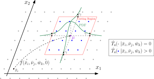
Figure 1. A 2-dimensional visualization of the cutting probability region (shown in red) with a cutting threshold of $\gamma$. The cutting region encloses representative post states (blue dots) that have non-zero probabilities in $\hat{T}_{\mathsf{x}}$. Other post states outside of the cutting region are considered to have zero probabilities in $\hat{T}_{\mathsf{x}}$.

Note that since $\mathsf{\Sigma}$ is fixed prior to running the algorithm, number of columns needed for a fixed $\gamma$ can be identified before launching the computation. We can then accurately allocate a uniform fixed number of memory locations for any tuple $(\bar{x}_{i},\bar{\nu}_{j},\bar{w}_{k})$ in $\hat{T}_{\mathsf{x}}$. Hence, there is no need for a dynamic sparse matrix data structure and $\hat{T}_{\mathsf{x}}$ is now a matrix with a dimension of $(n_{x}\times n_{\nu}\times n_{w},|\hat{X}^{\mathsf{\Sigma}}_{\gamma}|)$.

Remark 5.1.

Construction of $\hat{X}^{\mathsf{\Sigma}}_{\gamma}$ is practically a simple process. We start by solving the equation $\text{PDF}(x^{*}\,|\,0,\mathsf{\Sigma})=\gamma$ for $x^{*}\in\mathbb{R}^{n}_{>0}$ and computing the zero-mean cutting points at each dimension. Now, since the PDF is symmetric, one obtains

$$\centering\hat{X}^{\mathsf{\Sigma}}_{\gamma}=\{\bar{x}\in\hat{X}|\bar{x}\in[\![\mu-x^{*},\mu+x^{*}]\!]\}.\@add@centering$$

Remark 5.2.

The reduction in memory usage discussed in this subsection is tailored to Gaussian distributions for the sake of a better presentation of the idea. Users interested in adding additional distributions to AMYTISS have the option of providing a subroutine that describes how other distributions should behave in terms of required memory and with respect to the cutting threshold $\gamma$.

5.3. A Parallel Algorithm for Constructing Finite MDP $\widehat{\Sigma}$

We present a novel parallel algorithm (Algorithm 2) to efficiently construct and store $\hat{T}_{\mathsf{x}}$ as a successor to Algorithm 1. We employ the discussed enhancements in Subsections 5.1 and 5.2 within the proposed algorithm. We do not parallelize the for-loop in Algorithm 2, Step 2, to avoid excessive parallelism (i.e., we parallelize loops only over $X$ and $U$, but not over $W$). Note that, practically, for large-scale systems, $|\hat{X}\times\hat{U}|$ can reach up to billions. We are interested in the number of parallel threads that can be scheduled reasonably by available HW computing units.

Algorithm 2 Proposed parallel algorithm for computing $\hat{T}_{\mathsf{x}}$

0:  $\hat{X},\hat{U},\hat{W},\gamma$, and a noise covariance matrix $\mathsf{\Sigma}\in\mathbb{R}^{n\times n}$

0:  Transition probability matrix $\hat{T}_{\mathsf{x}}$ with the dimension of $(n_{x}\times n_{\nu}\times n_{w},|\hat{X}^{\mathsf{\Sigma},W}_{\gamma}|)$

1:  for all $(\bar{x},\bar{\nu})\in\hat{X}\times\hat{U}$ in parallel do

2:    for all $\bar{w}\in\hat{W}$ do

3:    Set $\mu=f(\bar{x},\bar{\nu},\bar{w})$

4:    Construct $\hat{X}^{\mathsf{\Sigma}}_{\gamma}$ as described in Remark 5.1

5:    for all $x^{*}\in\hat{X}^{\mathsf{\Sigma}}_{\gamma}$ do

6:     Set $\hat{T}_{\mathsf{x}}(x^{*}|\bar{x},\bar{\nu},\bar{w}):=\int_{\Xi(x^{*})}\text{PDF}(\mathsf{d}x|\mu,\mathsf{\Sigma})$

7:    end

8:   end

9:  end

6. Parallel Synthesis of Controllers

In this section, we employ dynamic programming to synthesize controllers for constructed finite MDPs $\widehat{\Sigma}$ satisfying safety, reachability, and reach-avoid properties [Sou14, SA13]. We first present the traditional serial algorithm in Algorithm 3. Note that if there are no disturbances in the given dynamics, Steps 15 and 16 of Algorithm 3 are to be excluded.

Algorithm 3 Traditional serial algorithm for controller synthesis satisfying safety, reachability and reach-avoid specifications

0:  $\hat{X}$, $\hat{U}$, $\hat{W}$, bounded time horizon $T_{d}$, $specs\in\{Safety,Reachability,$ $Reach$-$Avoid\}$, target set $\mathcal{T}$ (in case $specs=Reachability,Reach$-$Avoid$), and avoid set $\mathcal{A}$ (in case $specs=Reach$-$Avoid$).

0:  Optimal satisfaction probability $V_{v}$ at time step $T_{d}=1$, and optimal policy $\nu^{\star}$ corresponding to the optimal satisfaction probability.

1:  Compute $\hat{T}_{\mathsf{x}}$ as presented in Algorithm 1.

2:  if $specs==Safety$ do

3:    Set value function $V_{v}:=ones(n_{x},T_{d}+1)$

4:  else

5:    Compute a transition probability matrix $\hat{T}_{0\mathsf{x}}$ from $\hat{X}\backslash(\mathcal{T}\cup\mathcal{A})$ to $\mathcal{T}$

6:    Set $\hat{T}_{\mathsf{x}}$ to zero for any post-state in $(\mathcal{T}\cup\mathcal{A})$.

7:    Set value function $V_{v}:=zeros(n_{x},T_{d}+1)$

8:  end

9:   for $k=T_{d}:-1:1$ (backward in time) do

10:    if $specs==Safety$ do

11:     Set $V_{in}=\hat{T}_{\mathsf{x}}V_{v}(:~{}\!,k+1)$ {$V_{in}$ has the dimension of $(n_{x}\times n_{\nu}\times n_{w},1)$}

12:    else

13:     Set $V_{in}=\hat{T}_{0\mathsf{x}}+\hat{T}_{\mathsf{x}}V_{v}(:~{}\!,k+1)$ {$V_{in}$ has the dimension of $(n_{x}\times n_{\nu}\times n_{w},1)$}

14:    end

15:    Reshape $V_{in}$ to a matrix $\bar{V}_{in}$ of the dimension $(n_{x}\times n_{\nu},n_{w})$

16:    Minimize $\bar{V}_{in}$ with respect to disturbance set $\hat{W}$ as $V_{min}$

17:    Reshape $V_{min}$ to a matrix $\bar{V}_{min}$ of the dimension $(n_{x},n_{\nu})$

18:    Maximize $\bar{V}_{min}$ with respect to input set $\hat{U}$ as $V_{max}$ of the dimension $(n_{x},1)$

19:    Update $V_{v}(:,k):=V_{max}$

20:  end

The serial algorithm does, repetitively, matrix multiplications in each loop that corresponds to different time instance of the bounded time $T_{d}$. We cannot parallelize the for-loop in Step 9 over time-steps due to the data dependency, however, we can parallelize the contents of this loop by simply considering standard parallel algorithms for the matrix multiplication.

Algorithm 4 Proposed parallel algorithm for controller synthesis satisfying safety, reachability and reach-avoid specifications

0:  $\hat{X}$, $\hat{U}$, $\hat{W}$, bounded time horizon $T_{d}$, $specs\in\{Safety,Reachability,$ $Reach$-$Avoid\}$, target set $\mathcal{T}$ (in case $specs=Reachability,Reach$-$Avoid$), and avoid set $\mathcal{A}$ (in case $specs=Reach$-$Avoid$).

0:  Optimal satisfaction probability $V_{v}$ at time step $T_{d}=1$, and optimal policy $\nu^{\star}$ corresponding to the optimal satisfaction probability.

1:   Compute $\hat{T}_{\mathsf{x}}$ in parallel as presented in Algorithm 2.

2:  if $specs==Safety$ do

3:    Set value function $V_{v}:=ones(n_{x},T_{d}+1)$

4:  else

5:     Compute a transition probability matrix $\hat{T}_{0\mathsf{x}}$ from $\hat{X}\backslash(\mathcal{T}\cup\mathcal{A})$ to $\mathcal{T}$

6:    Set $\hat{T}_{\mathsf{x}}$ to zero for any post-state in $(\mathcal{T}\cup\mathcal{A})$.

7:    Set value function $V_{v}:=zeros(n_{x},T_{d}+1)$

8:  end

9:  for $k=T_{d}:-1:1$ (backward in time) do

10:    for all $(\bar{x},\bar{\nu})\in\hat{X}\times\hat{U}$ in parallel do

11:     for all $\bar{w}\in\hat{W}$

12:     Construct $\hat{X}^{\mathsf{\Sigma}}_{\gamma}$ as discussed in Subsection 5.2

13:      Set $V_{in}(\bar{x},\bar{\nu},\bar{w}):=\underset{x^{*}\in\hat{X}^{\mathsf{\Sigma}}_{\gamma}}{\sum}V_{v}(x^{*},k+1)T_{\mathsf{x}}(x^{*}|\bar{x},\bar{\nu},\bar{w})$

14:     if $specs==Reach$-$Avoid$ and $\bar{x}\not\in(\mathcal{T}\cup\mathcal{A})$ do

15:       Set $V_{in}(\bar{x},\bar{\nu},\bar{w}):=V_{in}(\bar{x},\bar{\nu},\bar{w})+T_{0\mathsf{x}}(\bar{x},\bar{\nu},\bar{w})$

16:     end

17:    end

18:   end

19:    for all $\bar{x}\in\hat{X}$ in parallel do

20:    Set $V_{v}(\bar{x},k):=\underset{\bar{\nu}\in\hat{U}}{\max}\{\underset{\bar{w}\in\hat{W}}{\min}\{V_{in}(\bar{x},\bar{\nu},\bar{w})\}\}$

21:    Set $\nu^{\star}(\bar{x},k):=\underset{\bar{\nu}\in\hat{U}}{\text{argmax}}\{\underset{\bar{w}\in\hat{W}}{\min}\{V_{in}(\bar{x},\bar{\nu},\bar{w})\}\}$

22:   end

23:  end

Algorithm 4 is a parallelization of Algorithm 3. Step 10 in Algorithm 4 is the parallel implementation of the matrix multiplication in Algorithm 3. Step 19 in Algorithm 4 selects and stores the input $\bar{\nu}$ that maximizes the probabilities of enforcing the specifications.

A significant reduction in the computation of the intermediate matrix $V_{in}$ is also introduced in Algorithm 4. In Algorithm 3, Step 11, the computation of $V_{in}$ requires a matrix multiplication between $T_{\mathsf{x}}$ (with a dimension of $(n_{x}\times n_{\nu}\times n_{w},n_{x})$) and $V_{v}(:,\cdot)$ (with a dimension of $(n_{x},1)$). On the other hand, in the parallel version in Algorithm 4, for each $\bar{w}$, the corresponding computation is done for $V_{in}$ such that each element, i.e., $V_{in}(\bar{x},\bar{\nu},\bar{w})$, requires only $|\hat{X}^{\mathsf{\Sigma}}_{\gamma}|$ scalar multiplications. Here, we clearly utilize the technique discussed in Subsection 5.2 to consider only those post states in the cutting region $\hat{X}^{\mathsf{\Sigma}}_{\gamma}$. Remember that other post states outside $\hat{X}^{\mathsf{\Sigma}}_{\gamma}$ are considered to have the probability zero which means we can avoid their scalar multiplications.

6.1. On-the-Fly Construction of $\hat{T}_{\mathsf{x}}$

In AMYTISS, we also use another technique that further reduces the required memory for computing $\hat{T}_{\mathsf{x}}$. We refer to this approach as on-the-fly abstractions (OFA). In OFA version of Algorithm 4, we skip computing and storing the MDP $\hat{T}_{\mathsf{x}}$ and the matrix $\hat{T}_{0\mathsf{x}}$ (i.e., Steps 1 and 5). We instead compute the required entries of $\hat{T}_{\mathsf{x}}$ and $\hat{T}_{0\mathsf{x}}$ on-the-fly as they are needed (i.e., Steps 13 and 15). This significantly reduces the required memory for $\hat{T}_{\mathsf{x}}$ and $\hat{T}_{0\mathsf{x}}$ but at the cost of repeated computation of their entries in each time step from $1$ to $T_{d}$. This gives the user an additional control over the trade-off between the computation time and memory.

6.2. Supporting Multiplicative Noises and Practical Distributions

AMYTISS natively supports multiplicative noises and practical distributions such as uniform, exponential, and beta distributions. The technique introduced in Subsection 5.2 for reducing the memory usage is also tuned for other distributions based on the support of their PDFs. Since AMYTISS is designed for extensibility, it allows also for customized distributions. Users need to specify their desired PDFs and hyper-rectangles enclosing their supports so that AMYTISS can include them in the parallel computation of $\hat{T}_{\mathsf{x}}$. Further details on specifying customized distributions are provided in the README file.

AMYTISS also supports multiplicative noises as introduced in (3.2). Currently, the memory reduction technique of Subsection 5.2 is disabled for systems with multiplicative noises. This means users should expect larger memory requirements for systems with multiplicative noises. However, users can still benefit from the proposed OFA version to compensate for the increase in memory requirement. We plan to include this feature for multiplicative noises in a future update of AMYTISS. Note that for a better demonstration, previous sections were presented by the additive noise and Gaussian normal PDF to introduce the concepts.

7. AMYTISS by Example

AMYTISS is self-contained and requires only a modern C++ compiler. It supports the three major operating systems: Windows, Linux and Mac OS. We tested AMYTISS on Windows 10 x64, MacOS Mojave, Ubuntu 16.04, and Ubuntu 18.04, and found no major computation time differences. Once compiled, utilizing AMYTISS is a matter of providing text configuration files and launching the tool. Please refer to the provided README file in the repository of AMYTISS for a general installation instruction.

For the sake of better illustrating the proposed algorithms and the usage of AMYTISS, we first introduce a simple 2-dimensional example. Consider a robot described by the following difference equations:

$$\begin{bmatrix}x_{1}(k+1)\\ x_{2}(k+1)\\ \end{bmatrix}=\begin{bmatrix}x_{1}(k)+\tau\nu_{1}(k)\text{cos}(\nu_{2}(k))+w(k)+\varsigma_{1}(k)\\ x_{2}(k)+\tau\nu_{2}(k)\text{sin}(\nu_{2}(k))+w(k)+\varsigma_{2}(k)\\ \end{bmatrix}\!\!,$$ (7.1)

where $(x_{1},x_{2})\in X:=[-10,10]^{2}$ is a state vector representing a spacial coordinate, $(\nu_{1},\nu_{2})\in U:=[-1,1]^{2}$ is an input vector, $w\in W:=[-1,1]$ is a disturbance, $(\varsigma_{1},\varsigma_{2})$ is a noise following a Gaussian distribution with the covariance matrix $\mathsf{\Sigma}:=\textsf{diag}(0.75,0.75)$, and $\tau:=10$ is a constant.

To construct MDPs approximating the system, we consider a state quantization parameter of $(0.5,0.5)$, an input quantization parameter of $(0.1,0.1)$, a disturbance quantization parameter of $0.2$, and a cutting probability threshold $\gamma$ of $0.001$. Using such quantization parameters, the number of state-input pairs $|\hat{X}\times\hat{U}|$ in $\widehat{\Sigma}$ is 203401. We use $|\hat{X}\times\hat{U}|$ as an indicator of the size of the system.

System descriptions and controller synthesis requirements are provided to AMYTISS as text configuration files. The configuration files of this example is located in the directory %AMYTISS%/examples/ex_toy_XXXX, where %AMYTISS% is the installation directory of AMYTISS and XXXX should be replaced by the controller synthesis specification of interest and can be any of: safety, reachability, or reach-avoid. For a detailed description of the key-value pairs in each configuration file, refer to the README file in the repository of AMYTISS.

7.1. Synthesis for Safety Specifications

We synthesize a controller for the robot system in (7.1) to keep the state of the robot inside $X$ within 8 time steps. The synthesized controller should enforce the safety specification in the presence of the disturbance and noise. The corresponding configuration file is located in file %AMYTISS%/examples/ex_toy_safety/toy2d.cfg, which describes the system in (7.1) and its safety requirement. To launch AMYTISS and run it for synthesizing the safety controller for this example, navigate to the install directory %AMYTISS% and run the command:

⬇

$ pfaces -CGH -d 1 -k amytiss.cpu@./kernel-pack -cfg ./examples/ex_toy_safety/toy2d.cfg -p

where pfaces calls pFaces, -CGH -d 1 asks pFaces to consider the first device from all CPU, GPU and HWA devices, -k amytiss.cpu@./kernel-pack asks pFaces to launch AMYTISS’s kernel from its main source folder, -cfg ./examples/ex_toy _safety/toy2d.cfg asks pFaces to hand the configuration file to AMYTISS, and -p asks pFaces to collect profiling information.

This launches AMYTISS to construct an MDP of the robot system and synthesize a safety controller for it. The results are stored in an output file specified in the configuration file. Using the provided MATLAB interface in AMYTISS, we visualize some transitions of the constructed MDP and show them in Figure 2. The used MATLAB script is located in %AMYTISS%/examples/ex_toy_safety/make_figs.m.

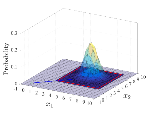
Figure 2. A visualization of transitions for one source state $x:=(0,0)$ and input $\nu=(0.7,0.8)$ of the MDP approximating the robot example. The green point is the source state, the transparent bell-like shape is the PDF and the red rectangle is the cutting region. Probabilities of reaching the partition elements inside the cutting regions are shown as bars below the PDF.

The output file contains also the control strategy which we use to simulate the closed-loop behavior of the system. Again, we rely on the the provided MATLAB interface in AMYTISS to simulate the closed-loop behavior. The MATLAB script in %AMYTISS%/examples/ex_toy_safety/closedloop.m simulates the system with random choices on $\bar{w}\in\hat{W}$ and random values for the noise according to the given covariance matrix. At each time step, the simulation queries the strategy from the output file and applies it to the system. We repeat the simulation 100 times. Figure 3 shows the closed-loop simulation results. Note that the input is always fixed at the time step $k=0$. This is because we store only one input, which is the one maximizing the probability of satisfaction. After the time step $k=0$ and due to the noise/disturbance, the system lands in different states which requires applying different inputs to satisfy the specification.

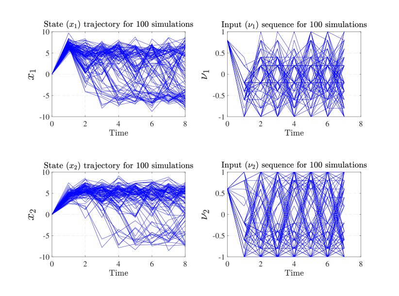
Figure 3. 100 different simulations of the closed-loop behavior of the robot under a safety controller synthesized for maintaining the robot inside $X$. At left, we show the state trajectory of the system at each time step. At right, we show the applied input at each time step. For the sake of readability, the input plots are shown as piece-wise linear signal.

7.2. Synthesis for Reach-Avoid Specifications

We synthesize a controller for the robot system in (7.1) to reach the set $[5,7]^{2}$ while avoiding the set $[-2,2]^{2}$ within 16 time steps. To launch AMYTISS and run it for synthesizing the reach-avoid controller for this example, navigate to the install directory %AMYTISS% and run the command:

⬇

$ pfaces -CGH -k amytiss.cpu@./kernel-pack -cfg ./examples/ex_toy_reachavoid/toy2d.cfg -d 1 -p

This launches AMYTISS to construct an MDP of the robot system and synthesize a reach-avoid controller for it. A MATLAB script simulates the closed-loop and it is located in %AMYTISS%/examples/ex_toy_reachavoid/closed
loop.m. This runs 9 different simulations from 9 different initial states. Figure 4 shows the closed-loop simulation results.

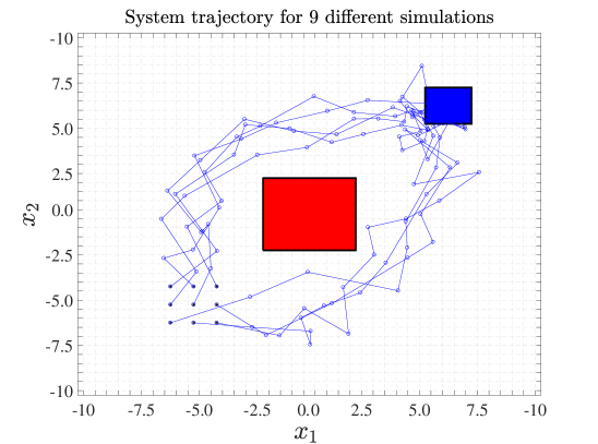
Figure 4. 9 different simulations of the closed-loop behavior of the robot example under a synthesized controller enforcing the robot to reach a target set while avoiding an avoid set. The 9 dots at the left bottom correspond to 9 initial states for 9 different simulation runs. The red rectangle is the avoid set of states. The blue rectangle is the target set of states.

8. Benchmarking and Case Studies

8.1. Controlling the Computational Complexities

AMYTISS implements scalable parallel algorithms that run on top of pFaces. Hence, users can utilize computing power in HPC platforms and cloud computing to scale the computation and control the computational complexities of their problems. We fix the system (i.e., the robot example) in hand and show how AMYTISS scales with respect to different computing platforms. Table 2 lists the HW configuration we use to benchmark AMYTISS. The devices range from local devices in laptops and desktop computers to advanced compute devices in Amazon AWS cloud computing services.

Table 2. HW configurations for benchmarking AMYTISS.

Id	Description	PEs	Frequency
CPU1	Local machine: Intel Xeon E5-1620	8	3.6 GHz
CPU2	Macbook Pro 15: Intel i9-8950HK	12	2.9 GHz
CPU3	AWS instance c5.18xlarge: Intel Xeon Platinum 8000	72	3.6 GHz
GPU1	Macbook Pro 15 laptop laptop: Intel UHD Graphics 630	23	0.35 GHz
GPU2	Macbook Pro 15 laptop: AMD Radeon Pro Vega 20	1280	1.2 GHz
GPU3	AWS p3.2xlarge instance: NVIDIA Tesla V100	5120	0.8 GHz

Table 4 shows the benchmarking results running AMYTISS with these HWCs for several case studies and makes comparisons between AMYTISS, FAUST², and StocHy. We employ a machine with Windows operating system (Intel i7@3.6GHz CPU and 16 GB of RAM) for FAUST², and StocHy. It should be mentioned that FAUST² predefines a minimum number of representative points based on the desired abstraction error, and accordingly the computation time and memory usage reported in Table 4 are based on the minimum number of representative points. In addition, to have a fair comparison, we run all the case studies with additive noises since neither FAUST² nor StocHy supports multiplicative noises.

For each HWC, we show the time in seconds to solve the problem. Clearly, employing HWCs with more PEs reduces the time to solve the problem. This is a strong indication for the scalability of the proposed algorithms. This also becomes very useful in real-time applications, where users can control the computation time of their problems by adding more resources. Since, AMYTISS is the only tool that can utilize the reported HWCs, we do not compare it with other similar tools.

To show the applicability of our results to large-scale stochastic systems, we apply our proposed techniques to several physical case studies. First, we synthesize a controller for $3$- and $5$-dimensional room temperature networks to keep temperature of rooms in a comfort zone. Then we synthesize a controller for road traffic networks with $3$ and $5$ dimensions to keep the density of the traffic below some level. We then consider $3$- and $7$-dimensional nonlinear models of an autonomous vehicle and synthesize reach-avoid controllers to automatically park the vehicles. For each case study, we compare our tool with FAUST² and StocHy and report the technical details in Table 4.

8.2. Room Temperature Network

8.2.1. 5-Dimensional System.

We first apply our results to the temperature regulation of $5$ rooms each equipped with a heater and connected on a circle. The model of this case study is borrowed from [LSZ18b]. The evolution of temperatures $T_{x_{i}}$ can be described by individual rooms as

$$\Sigma_{\mathfrak{a}_{i}}:\left\{\begin{array}[]{l}T_{x_{i}}(k+1)=a_{ii}T_{x_{i}}(k)+\gamma T_{h}\nu_{i}(k)+\eta w_{i}(k)+\beta T_{ei}+0.01\varsigma_{i}(k),i\in\{1,3\},\\ T_{x_{i}}(k+1)=b_{ii}T_{x_{i}}(k)+\eta w_{i}(k)+\beta T_{ei}+0.01\varsigma_{i}(k),i\in\{2,4,5\},\\ y_{i}(k)=T_{x_{i}}(k),\\ \end{array}\right.$$

where $a_{ii}=(1-2\eta-\beta-\gamma\nu_{i}(k))$, $b_{ii}=(1-2\eta-\beta)$, and $w_{i}(k)=T_{x_{i-1}}(k)+T_{x_{i+1}}(k)$ (with $T_{x_{0}}=T_{x_{n}}$ and $T_{x_{n+1}}=T_{x_{1}}$). Parameters $\eta=0.3$, $\beta=0.022$, and $\gamma=0.05$ are conduction factors, respectively, between rooms $i\pm 1$ and the room $i$, between the external environment and the room $i$, and between the heater and the room $i$. Moreover, $T_{ei}=-1\,^{\circ}C$, $T_{h}=50\,^{\circ}C$ are outside and heater temperatures, and $T_{i}(k)$ and $\nu_{i}(k)$ are taking values in sets $[19,21]$ and $[0,1]$, respectively, $\forall i\in\{1,\ldots,n\}$.

Let us now synthesize a controller for $\Sigma_{\mathfrak{a}}$ via the abstraction $\widehat{\Sigma}_{\mathfrak{a}}$ such that the controller maintains the temperature of any room in the safe set $[19,21]$ for at least $8$ time steps.

8.2.2. 3-Dimensional System.

We also apply our algorithms to a smaller version of this case study ($3$-dimensional system) with the results reported in Table 4.

8.3. Road Traffic Network

8.3.1. 5-Dimensional System.

Consider a road traffic network divided in $5$ cells of $500$ meters with $2$ entries and $2$ ways out, as schematically depicted in Figure 5. The model of this case study is borrowed from [LCGG13] by including the stochasticity in the model as the additive noise.

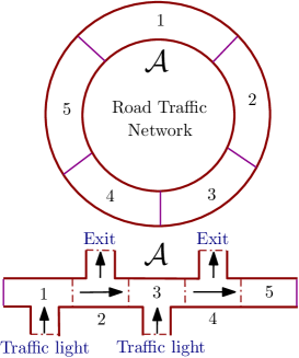
Figure 5. Model of a road traffic network composed of $5$ cells of $500$ meters with $2$ entries and $2$ ways out.

The two entries are controlled by traffic lights, denoted by $\nu_{1}$ and $\nu_{3}$, that enable (green light) or not (red light) the vehicles to pass. In this model, the length of a cell is in kilometers [km] and the flow speed of vehicles is $100$ kilometers per hour [km/h]. Moreover, during the sampling time interval $\tau=6.48$ seconds, it is assumed that $6$ vehicles pass the entry controlled by the light $\nu_{1}$, $8$ vehicles pass the entry controlled by the light $\nu_{3}$, and one quarter of vehicles that leave cells $1$ and $3$ goes out on the first exit (its ratio denoted by $q$). We want to observe the density of the traffic $x_{i}$, given in vehicles per cell, for each cell $i$ of the road. The model of cells is described by:

$$x_{1}(k+1) =(1-\frac{\tau v_{1}}{L_{1}})x_{1}(k)+\frac{\tau v_{5}}{L_{5}}w_{1}(k)+6\nu_{1}(k)+0.7\varsigma_{1}(k),$$

$$x_{i}(k+1) =(1-\frac{\tau v_{i}}{L_{i}}-q)x_{i}(k)+\frac{\tau v_{i-1}}{L_{i-1}}w_{i}(k)+0.7\varsigma_{i}(k),\quad i\in\{2,4\},$$

$$x_{3}(k+1) =(1-\frac{\tau v_{3}}{L_{3}})x_{3}(k)+\frac{\tau v_{2}}{L_{2}}w_{3}(k)+8\nu_{3}(k)+0.7\varsigma_{3}(k),$$

$$x_{5}(k+1) =(1-\frac{\tau v_{5}}{L_{5}})x_{5}(k)+\frac{\tau v_{4}}{L_{4}}w_{5}(k)+0.7\varsigma_{5}(k),$$

where $w_{i}(k)=x_{i-1}(k)$ (with $x_{0}=x_{5}$). We are interested first in constructing the finite MDP of the given $5$-dimensional system and then synthesizing policies keeping the density of the traffic lower than $10$ vehicles per cell.

For this example, we have $X:=[0,10]^{5}$ with a quantization parameter of $(0.37,0.37,0.37,0.37,0.37)$, $U=[0,1]^{2}$ with a quantization parameter of $(1,1)$, a noise covariance matrix $\mathsf{\Sigma}:=\textsf{diag}(0.7,0.7,0.7,0.7,0.7)$, and a cutting probability level $\gamma$ of $2e-2$.

8.3.2. 3-Dimensional System.

We also apply our algorithms to the same case study but with $3$ dimensions for the sake of benchmarking.

8.4. Autonomous Vehicle

8.4.1. 7-Dimensional BMW $320$i.

Here, to show the applicability of our approaches to nonlinear models, we consider a vehicle described by the following hybrid $7$-dimensional nonlinear single track (ST) model of a BMW $320$i car [Alt19, Section 5.1] by including the stochasticity inside the dynamics as the additive noise:

For $|x_{4}(k)|<0.1$:

$$x_{i}(k+1) =x_{i}(k)+\tau a_{i}(k)+R_{i}\varsigma_{i}(k),\quad i\in\{1,\dots,7\}\backslash\{3,4\},$$

$$x_{3}(k+1) =x_{3}(k)+\tau\text{Sat}_{1}(\nu_{1})+0.2\varsigma_{3}(k),$$

$$x_{4}(k+1) =x_{4}(k)+\tau\text{Sat}_{2}(\nu_{2})+0.1\varsigma_{4}(k),$$

for $|x_{4}(k)|\geq 0.1$:

$$x_{i}(k+1) =x_{i}(k)+\tau b_{i}(k)+R_{i}\varsigma_{i}(k),\quad i\in\{1,\dots,7\}\backslash\{3,4\},$$

$$x_{3}(k+1) =x_{3}(k)+\tau\text{Sat}_{1}(\nu_{1})+0.2\varsigma_{3}(k),$$

$$x_{4}(k+1) =x_{4}(k)+\tau\text{Sat}_{2}(\nu_{2})+0.1\varsigma_{4}(k),$$

where,

$$R_{1} =R_{2}=0.25,\quad R_{5}=R_{6}=R_{7}=0.2,\quad a_{1}=x_{4}\text{cos}(x_{5}(k)),\quad a_{2}=x_{4}\text{sin}(x_{5}(k)),$$

$$\quad a_{5} =\frac{x_{4}}{l_{wb}}\text{tan}(x_{3}(k)),\quad a_{6}=\frac{\nu_{2}(k)}{l_{wb}}\text{tan}(x_{3}(k))+\frac{x_{4}}{l_{wb}\text{cos}^{2}(x_{3}(k))}\nu_{1}(k),\quad a_{7}=0,$$

$$b_{1} =x_{4}(k)\text{cos}(x_{5}(k)+x_{7}(k)),\quad b_{2}=x_{4}(k)\text{sin}(x_{5}(k)+x_{7}(k)),\quad b_{5}=x_{6}(k),$$

$$b_{6} =\frac{\bar{\mu}m}{I_{z}(l_{r}+l_{f})}(l_{f}C_{S,f}(gl_{r}-\nu_{2}(k)h_{cg})x_{3}(k)+(l_{r}C_{S,r}(gl_{f}+\nu_{2}(k)h_{cg})-l_{f}C_{S,f}(gl_{r}-\nu_{2}(k)h_{cg}))x_{7}(k)$$

$$\quad-(l_{f}^{2}C_{S,f}(gl_{r}-\nu_{2}(k)h_{cg})+l_{r}^{2}C_{S,r}(gl_{f}+\nu_{2}(k)h_{cg}))\frac{x_{6}(k)}{x_{4}(k)}),$$

$$b_{7} =\frac{\bar{\mu}_{f}}{x_{4}(k)(l_{r}+l_{f})}(C_{S,f}(gl_{r}-\nu_{2}(k)h_{cg})x_{3}(k)+(C_{S,r}(gl_{f}+\nu_{2}(k)h_{cg})+C_{S,f}(gl_{r}-\nu_{2}(k)h_{cg}))x_{7}(k)$$

$$\quad-(l_{f}C_{S,f}(gl_{r}-\nu_{2}(k)h_{cg})-l_{r}C_{S,r}(gl_{f}+\nu_{2}(k)h_{cg}))\frac{x_{6}(k)}{x_{4}(k)})-x_{6}(k).$$

Here, $\text{Sat}_{1}(\cdot)$ and $\text{Sat}_{2}(\cdot)$ are input saturation functions introduced in [Alt19, Section 5.1], $x_{1}$ and $x_{2}$ are the position coordinates, $x_{3}$ is the steering angle, $x_{4}$ is the heading velocity, $x_{5}$ is the yaw angle, $x_{6}$ is the yaw rate, and $x_{7}$ is the slip angle. Variables $\nu_{1}$ and $\nu_{2}$ are inputs and they control the steering angle and heading velocity, respectively.

The model takes into account the tire slip making it a good candidate for studies that consider planning of evasive maneuvers that are very close to physical limits. We consider an update period $\tau=0.1$ seconds and the following parameters for a BMW $320$i car: $l_{wb}=2.5789$ as the wheelbase, $m=1093.3$ [kg] as the total mass of the vehicle, $\bar{\mu}=1.0489$ as the friction coefficient, $l_{f}=1.156$ [m] as the distance from the front axle to the center of gravity (CoG), $l_{r}=1.422$ [m] as the distance from the rear axle to CoG, $h_{cg}=0.6137$ [m] as the hight of CoG, $I_{z}=1791.6$ [kg m²] as the moment of inertia for entire mass around $z$ axis, $C_{S,f}=20.89$ [$1$/rad] as the front cornering stiffness coefficient, and $C_{S,r}=20.89$ [$1$/rad] as the rear cornering stiffness coefficient.

To construct a finite MDP $\widehat{\Sigma}_{\mathfrak{a}}$, we consider a bounded version of the state set $X:=[-10.0,10.0]\times[-10.0,10.0]\times[-0.40,0.40]\times[-2,2]\times[-0.3,0.3]\times[-0.4,0.4]\times[-0.04,0.04]$, a state discretization vector $[4.0;4.0;0.2;1.0;0.1;0.2;\\ 0.02]$, an input set $U:=[-0.4,0.4]\times[-4,4]$, and an input discretization vector $[0.2;2.0]$.

We are interested in an autonomous operation of the vehicle. The vehicle should park itself automatically in the parking lot located in the projected set $[-1.5,0.0]\times[0.0,1.5]$ within 32 time steps. The vehicle should avoid hitting a barrier represented by the set $[-1.5,0.0]\times[-0.5,0.0]$.

8.4.2. 3-Dimensional Autonomous Vehicle.

We also apply our algorithms to a $3$-dimensional autonomous vehicle [RWR16, Section IX-A] for the sake of benchmarking.

8.5. Benchmark in StocHy

We benchmark our results against the ones provided by StocHy [CA19]. We employ the same case study as in [CA19, Case study 3] which starts from 2-dimensional to $12$-dimensional continuous-space systems with the same parameters.

To have a fair comparison, we utilize a machine with the same configuration as the one employed in [CA19] (a laptop having an Intel Core i$7-8550$U CPU at $1.80$GHz with $8$ GB of RAM). We build a finite MDP for the given model and compare our computation time with the results provided by StocHy.

Table 3 shows the comparison between StocHy and AMYTISS. StocHy suffers significantly from the state-explosion problem as seen from its exponentially growing computation time. AMYTISS, on the other hand, outperforms StocHy and can handle bigger systems using the same hardware. This comparison shows speedups up to maximum $375$ times for the $12$-dimensional system. Note that we only reported up to 12-dimensions but AMYTISS can readily go beyond this limit for this example. For instance, AMYTISS managed to handle the 20-dimensional version of this system in 1572 seconds using an NVIDIA Tesla V100 GPU in Amazon AWS.

Table 3. Comparison between StocHy and AMYTISS for a continuous-space system with dimensions up to 12. The reported system is autonomous and, hence, $\hat{U}$ is singleton. $|\hat{X}|$ refers to the size of the system.

Dimension	2	3	4	5	6	7	8	9	10	11	12
$|\hat{X}|$	4	8	16	32	64	128	265	512	1024	2048	4096
Time (s) - StocHy	0.015	0.08	0.17	0.54	2.17	9.57	40.5	171.6	385.5	1708.2	11216
Time (s) - AMYTISS	0.02	0.92	0.20	0.47	1.02	1.95	3.52	6.32	10.72	17.12	29.95

Readers are highly advised to pay attention to the size of the system $|\hat{X}\times\hat{U}|$ (or $|\hat{X}|$ when $\hat{U}$ is singleton), not to its dimension. Actually, here, the 12-dimensional system, which has a size of 4096 state-input pairs is much smaller than the 2-dimensional illustrative example we introduced in Section 7, which has a size of 203401 state-input pairs. The current example has a small size due to the very coarse quantization parameters and the tight bounds used to quantize $X$.

As seen in Table 4, AMYTISS outperforms FAUST² and StocHy in all the case studies (maximum speedups up to $692000$ times). Moreover, AMYTISS is the only tool that can utilize the available HW resources. The OFA feature in AMYTISS reduces dramatically the required memory, while still solves the problems in a reasonable time. FAUST² and StocHy fail to solve many of the problems since they lack the native support for nonlinear systems, they require large amounts of memory, or they do not finish computing within 24 hours.

Table 4. Comparison between AMYTISS, FAUST² and StocHy based on their native features for several (physical) case studies. CSB refers to the continuous-space benchmark provided in [CA19]. $\dagger$ refers to cases when we run AMYTISS with the OFA algorithm. N/M refers to the situation when there is not enough memory to run the case study. N/S refers to the lack of native support for nonlinear systems. (Kx) refers to an $1000$-times speedup. The presented speedup is the maximum speedup value across all reported devices. The required memory usage and computation time for FAUST² and StocHy are reported for just constructing finite MDPs. The reported times and memories are respectively in seconds and MB, unless other units are denoted.

				AMYTISS (time)							FAUST2		StocHy		Speedup w.r.t
Problem	Spec.	$|\hat{X}\times\hat{U}|$	$T_{d}$	Mem.	CPU1	CPU2	CPU3	GPU1	GPU2	GPU3	Mem.	Time	Mem.	Time	FAUST	StocHy
$2$-d StocHy CSB	Safety	4	6	$\leq$ 1.0	$\leq$ 1.0	$\leq$ 1.0	$\leq$ 1.0	$\leq$ 1.0	$\leq$ 1.0	0.0001	$\leq$ 1.0	0.002	8.5	0.015	20 x	150 x
$3$-d StocHy CSB	Safety	8	6	$\leq$ 1.0	$\leq$ 1.0	$\leq$ 1.0	$\leq$ 1.0	$\leq$ 1.0	$\leq$ 1.0	0.0001	$\leq$ 1.0	0.002	8.5	0.08	20 x	800 x
$4$-d StocHy CSB	Safety	16	6	$\leq$ 1.0	$\leq$ 1.0	$\leq$ 1.0	$\leq$ 1.0	$\leq$ 1.0	$\leq$ 1.0	0.0002	$\leq$ 1.0	0.01	8.5	0.17	50 x	850 Kx
$5$-d StocHy CSB	Safety	32	6	$\leq$ 1.0	$\leq$ 1.0	$\leq$ 1.0	$\leq$ 1.0	$\leq$ 1.0	$\leq$ 1.0	0.0003	$\leq$ 1.0	0.01	8.7	0.54	33 x	1.8 Kx
$6$-d StocHy CSB	Safety	64	6	$\leq$ 1.0	$\leq$ 1.0	$\leq$ 1.0	$\leq$ 1.0	$\leq$ 1.0	$\leq$ 1.0	0.0006	4.251	1.2	9.6	2.17	2.0 Kx	3.6 Kx
$7$-d StocHy CSB	Safety	128	6	$\leq$ 1.0	$\leq$ 1.0	$\leq$ 1.0	$\leq$ 1.0	$\leq$ 1.0	$\leq$ 1.0	0.0012	38.26	6	12.9	9.57	5 Kx	7.9 Kx
$8$-d StocHy CSB	Safety	256	6	$\leq$ 1.0	$\leq$ 1.0	$\leq$ 1.0	$\leq$ 1.0	$\leq$ 1.0	$\leq$ 1.0	0.0026	344.3	37	26.6	40.5	14.2 Kx	15.6 Kx
$9$-d StocHy CSB	Safety	512	6	1.0	$\leq$ 1.0	$\leq$ 1.0	$\leq$ 1.0	$\leq$ 1.0	$\leq$ 1.0	0.0057	3 GB	501	80.7	171.6	87.8 Kx	30.1 Kx
$10$-d StocHy CSB	Safety	1024	6	4.0	$\leq$ 1.0	$\leq$ 1.0	$\leq$ 1.0	$\leq$ 1.0	$\leq$ 1.0	0.0122	N/M		297.5	385.5	N/A	32 Kx
$11$-d StocHy CSB	Safety	2048	6	16.0	1.0912	$\leq$ 1.0	$\leq$ 1.0	$\leq$ 1.0	$\leq$ 1.0	0.0284	N/M		1 GB	1708.2	N/A	60 Kx
$12$-d StocHy CSB	Safety	4096	6	64.0	4.3029	4.1969	$\leq$ 1.0	$\leq$ 1.0	$\leq$ 1.0	0.0624	N/M		4 GB	11216	N/A	179 Kx
$13$-d StocHy CSB	Safety	8192	6	256.0	18.681	19.374	1.8515	1.6802	$\leq$ 1.0	0.1277	N/M		N/A	$\geq$ 24h	N/A	$\geq$676 Kx
$14$-d StocHy CSB	Safety	16384	6	1024.0	81.647	94.750	7.9987	7.3489	6.1632	0.2739	N/M		N/A	$\geq$ 24h	N/A	$\geq$320 Kx
$2$-d Robot$\dagger$	Safety	203401	8	$\leq$ 1.0	8.5299	5.0991	0.7572	$\leq$ 1.0	$\leq$ 1.0	0.0154	N/A		N/A		N/A	N/A
$2$-d Robot	R.Avoid	741321	16	482.16	48.593	18.554	4.5127	2.5311	3.4353	0.3083	N/S		N/S		N/A	N/A
$2$-d Robot$\dagger$	R.Avoid	741321	16	4.2484	132.10	41.865	11.745	5.3161	3.6264	0.1301	N/A		N/A		N/A	N/A
$3$-d Room Temp.	Safety	7776	8	6.4451	0.1072	0.0915	0.0120	$\leq$ 1.0	$\leq$ 1.0	0.0018	3.12	1247	N/M		692 Kx	N/A
$3$-d Room Temp.$\dagger$	Safety	7776	8	$\leq$ 1.0	0.5701	0.3422	0.0627	$\leq$ 1.0	$\leq$ 1.0	0.0028	N/A		N/A		N/A	N/A
$5$-d Room Temp.	Safety	279936	8	3338.4	200.00	107.93	19.376	10.084	N/M	1.8663	2 GB	3248	N/M		1740 x	N/A
$5$-d Room Temp.$\dagger$	Safety	279936	8	1.36	716.84	358.23	63.758	30.131	22.334	0.5639	N/A		N/A		N/A	N/A
$3$-d Road Traffic	Safety	2125764	16	1765.7	29.200	131.30	3.0508	5.7345	10.234	1.2895	N/M		N/M		N/A	N/A
$3$-d Road Traffic$\dagger$	Safety	2125764	16	14.19	160.45	412.79	13.632	12.707	11.657	0.3062	N/A		N/A		N/A	N/A
$5$-d Road Traffic	Safety	68841472	7	8797.4	N/M	537.91	38.635	N/M	N/M	4.3935	N/M		N/M		N/A	N/A
$5$-d Road Traffic$\dagger$	Safety	68841472	7	393.9	1148.5	1525.1	95.767	44.285	36.487	0.7397	N/A		N/A		N/A	N/A
$3$-d Vehicle	R.Avoid	1528065	32	1614.7	2.5h	1.1h	871.89	898.38	271.41	10.235	N/S		N/S		N/A	N/A
$3$-d Vehicle$\dagger$	R.Avoid	1528065	32	11.17	2.8h	1.9h	879.78	903.2	613.55	107.68	N/A		N/A		N/A	N/A
$7$-d BMW $320$i	R.Avoid	3937500	32	10169.4	N/M	$\geq$ 24h	21.5h	N/M	N/M	825.62	N/S		N/S		N/A	N/A
$7$-d BMW $320$i$\dagger$	R.Avoid	3937500	32	30.64	$\geq$ 24h	$\geq$ 24h	$\geq$ 24h	$\geq$ 24h	$\geq$ 24h	1251.7	N/A		N/A		N/A	N/A

9. Discussion and Future Work

In this paper, we introduced AMYTISS as a software tool for parallel automated controller synthesis of large-scale discrete-time stochastic control systems. This tool is developed in C++/OpenCL for constructing finite MDPs and synthesizing controllers satisfying some high-level specifications. The tool can run in HPC platforms together with cloud computing services to reduce the problem of state-explosion. We proposed parallel algorithms to target HPC platforms and then implemented them within AMYTISS. As illustrated, AMYTISS significantly outperforms FAUST² and StocHy w.r.t. the computation time and memory usage. Providing a tool for large-scale continuous-time stochastic control systems is under investigation as a future work.

10. Acknowledgment

The authors would like to thank Thomas Gabler for his help in implementing traditional serial algorithms for the purpose of analysis and then comparing with the parallel ones.

^∗Both authors have contributed equally.

References

- [ABC+18] A. Abate, H. Blom, N. Cauchi, S. Haesaert, A. Hartmanns, K. Lesser, M. Oishi, V. Sivaramakrishnan, S. Soudjani, C. I. Vasile, et al. ARCH-COMP18 category report: Stochastic modelling. In ARCH@ ADHS, pages 71–103, 2018.
- [ABC+19] A. Abate, H. Blom, N. Cauchi, K. Degiorgio, M. Fränzle, E. M. Hahn, S. Haesaert, H. Ma, M. Oishi, C. Pilch, et al. ARCH-COMP19 category report: Stochastic modelling. EPiC Series in Computing, 61:62–102, 2019.
- [Alt19] M. Althof. Commonroad: Vehicle models (version 2018a). Tech. rep. In Technical University of Munich, 85748 Garching, Germany (October 2018), https://commonroad.in.tum.de. 2019.
- [BK08] C. Baier and J.-P. Katoen. Principles of model checking. MIT press, 2008.
- [BS96] D. P. Bertsekas and S. E. Shreve. Stochastic Optimal Control: The Discrete-Time Case. Athena Scientific, 1996.
- [CA19] N. Cauchi and A. Abate. StocHy: Automated verification and synthesis of stochastic processes. In TACAS’19, volume 11428 of Lecture Notes in Computer Science, pages 247–264. 2019.
- [HH14] A. Hartmanns and H. Hermanns. The modest toolset: An integrated environment for quantitative modelling and verification. In International Conference on Tools and Algorithms for the Construction and Analysis of Systems, pages 593–598, 2014.
- [HS18] Sofie Haesaert and Sadegh Soudjani. Robust dynamic programming for temporal logic control of stochastic systems. CoRR, abs/1811.11445, 2018.
- [Jaj92] Joseph Jaja. An introduction to parallel algorithms. Addison-Wesley, 1992.
- [Kal97] O. Kallenberg. Foundations of modern probability. Springer-Verlag, New York, 1997.
- [KDS+11] M. Kamgarpour, J. Ding, S. Summers, A. Abate, J. Lygeros, and C. Tomlin. Discrete time stochastic hybrid dynamical games: Verification & controller synthesis. In Proceedings of the 50th IEEE Conference on Decision and Control and European Control Conference, pages 6122–6127, 2011.
- [KNP02] M. Kwiatkowska, G. Norman, and D. Parker. PRISM: Probabilistic symbolic model checker. In Proceedings of the International Conference on Modelling Techniques and Tools for Computer Performance Evaluation, pages 200–204, 2002.
- [KZ19] Mahmoud Khaled and Majid Zamani. pFaces: An acceleration ecosystem for symbolic control. In Proceedings of the 22nd ACM International Conference on Hybrid Systems: Computation and Control, pages 252–257, 2019.
- [Lav19] A. Lavaei. Automated Verification and Control of Large-Scale Stochastic Cyber-Physical Systems: Compositional Techniques. PhD thesis, Technische Universität München, Germany, 2019.
- [LCGG13] E.l Le Corronc, A. Girard, and G. Goessler. Mode sequences as symbolic states in abstractions of incrementally stable switched systems. In Proceedings of the 52th IEEE Conference on Decision and Control, pages 3225–3230, 2013.
- [LSMZ17] A. Lavaei, S. Soudjani, R. Majumdar, and M. Zamani. Compositional abstractions of interconnected discrete-time stochastic control systems. In Proceedings of the 56th IEEE Conference on Decision and Control, pages 3551–3556, 2017.
- [LSZ18a] A. Lavaei, S. Soudjani, and M. Zamani. Compositional synthesis of finite abstractions for continuous-space stochastic control systems: A small-gain approach. In Proceedings of the 6th IFAC Conference on Analysis and Design of Hybrid Systems, volume 51, pages 265–270, 2018.
- [LSZ18b] A. Lavaei, S. Soudjani, and M. Zamani. From dissipativity theory to compositional construction of finite Markov decision processes. In Proceedings of the 21st ACM International Conference on Hybrid Systems: Computation and Control, pages 21–30, 2018.
- [LSZ19a] A. Lavaei, S. Soudjani, and M. Zamani. Compositional abstraction-based synthesis of general MDPs via approximate probabilistic relations. arXiv: 1906.02930, 2019.
- [LSZ19b] A. Lavaei, S. Soudjani, and M. Zamani. Compositional construction of infinite abstractions for networks of stochastic control systems. Automatica, 107:125–137, 2019.
- [LSZ19c] A. Lavaei, S. Soudjani, and M. Zamani. Compositional synthesis of not necessarily stabilizable stochastic systems via finite abstractions. In Proceedings of the 18th European Control Conference, pages 2802–2807, 2019.
- [LSZ20a] A. Lavaei, S. Soudjani, and M. Zamani. Compositional abstraction-based synthesis for networks of stochastic switched systems. Automatica, 114, 2020.
- [LSZ20b] A. Lavaei, S. Soudjani, and M. Zamani. Compositional abstraction of large-scale stochastic systems: A relaxed dissipativity approach. Nonlinear Analysis: Hybrid Systems, 36, 2020.
- [LSZ20c] A. Lavaei, S. Soudjani, and M. Zamani. Compositional (in)finite abstractions for large-scale interconnected stochastic systems. IEEE Transactions on Automatic Control, DOI: 10.1109/TAC.2020.2975812, 2020.
- [LTS05] W. Li, E. Todorov, and R. E. Skelton. Estimation and control of systems with multiplicative noise via linear matrix inequalities. In Proceedings of the American Control Conference, pages 1811–1816, 2005.
- [LZ19a] A. Lavaei and M. Zamani. Compositional construction of finite MDPs for large-scale stochastic switched systems: A dissipativity approach. Proceedings of the 15th IFAC Symposium on Large Scale Complex Systems: Theory and Applications, 52(3):31–36, 2019.
- [LZ19b] A. Lavaei and M. Zamani. Compositional verification of large-scale stochastic systems via relaxed small-gain conditions. In Proceedings of the 58th IEEE Conference on Decision and Control, pages 2574–2579, 2019.
- [MSSM19] K. Mallik, A. Schmuck, S. Soudjani, and R. Majumdar. Compositional synthesis of finite-state abstractions. IEEE Transactions on Automatic Control, 64(6):2629–2636, 2019.
- [Pnu77] A. Pnueli. The temporal logic of programs. In Proceedings of the 18th Annual Symposium on Foundations of Computer Science, pages 46–57, 1977.
- [RWR16] G. Reissig, A. Weber, and M. Rungger. Feedback refinement relations for the synthesis of symbolic controllers. IEEE Transactions on Automatic Control, 62(4):1781–1796, 2016.
- [SA13] S. Soudjani and A. Abate. Adaptive and sequential gridding procedures for the abstraction and verification of stochastic processes. SIAM Journal on Applied Dynamical Systems, 12(2):921–956, 2013.
- [SAM15] S. Soudjani, A. Abate, and R. Majumdar. Dynamic Bayesian networks as formal abstractions of structured stochastic processes. In Proceedings of the 26th International Conference on Concurrency Theory, pages 1–14, 2015.
- [SGA15] S. Soudjani, C. Gevaerts, and A. Abate. FAUST: Formal abstractions of uncountable-state stochastic processes. In TACAS’15, volume 9035 of Lecture Notes in Computer Science, pages 272–286. 2015.
- [Sou14] S. Soudjani. Formal Abstractions for Automated Verification and Synthesis of Stochastic Systems. PhD thesis, Technische Universiteit Delft, The Netherlands, 2014.
- [SZ15] F. Shmarov and P. Zuliani. ProbReach: verified probabilistic delta-reachability for stochastic hybrid systems. In Proceedings of the 18th International Conference on Hybrid Systems: Computation and Control, pages 134–139, 2015.
- [VGO19] A. P. Vinod, J. D. Gleason, and M. M. Oishi. SReachTools: A MATLAB stochastic reachability toolbox. In Proceedings of the 22nd ACM International Conference on Hybrid Systems: Computation and Control, pages 33–38, 2019.
- [WZK+15] Q. Wang, P. Zuliani, S. Kong, S. Gao, and E. M. Clarke. SReach: A probabilistic bounded delta-reachability analyzer for stochastic hybrid systems. In Proceedings of the International Conference on Computational Methods in Systems Biology, pages 15–27, 2015.