Magnetic circular dichroism spectra from resonant and damped coupled cluster response theory

Abstract

A computational expression for the Faraday ${\mathcal{A}}$ term of magnetic circular dichroism (MCD) is derived within coupled cluster response theory and alternative computational expressions for the ${\mathcal{B}}$ term are discussed. Moreover, an approach to compute the (temperature-independent) MCD ellipticity in the context of coupled cluster damped response is presented, and its equivalence with the stick-spectrum approach in the limit of infinite lifetimes is demonstrated. The damped response approach has advantages for molecular systems or spectral ranges with a high density of states. Illustrative results are reported at the coupled cluster singles and doubles level and compared to time-dependent density functional theory results.

I Introduction

In magnetic circular dichroism (MCD) spectroscopy, the sample is probed with circularly polarized light in presence of a relatively strong magnetic field oriented parallel to the direction of propagation of the light beam. The external magnetic field induces a differential absorption of the right- and left- circularly polarized light. Mason (2007) MCD can provide insight to the geometric, electronic, and magnetic properties of chemical systems. The applied magnetic field couples to the (spin and/or orbital) angular momentum, lifting the degeneracies among ground and excited states (by Zeeman splitting), and giving rise to additional spectroscopic features compared to the zero-field case. Since the MCD spectral features are signed and depend upon molecular magnetic moments in electronic states and the direction of the field, MCD yields additional information when combined with conventional absorption spectroscopy. MCD spectra can be obtained from gases, solutions, or isotropic solids. Also, MCD can be observed for any sample of molecules independent of whether they are chiral or not. One can use MCD to study molecules of high symmetry, and to probe degenerate electronic ground and excited states.

About fifty years ago, Buckingham and Stephens Buckingham and Stephens (1966) described in an elegant and incisive way the theoretical foundation of MCD. For an electronic transition, the intensity of the signal is given by the contribution of three effects called ${\mathcal{A}}$, ${\mathcal{B}}$ and ${\mathcal{C}}$ terms. The ${\mathcal{A}}$ term originates from the Zeeman splitting of degenerate excited states. The ${\mathcal{B}}$ term arises from the mixing of the zero-field wavefunctions between nondegenerate states in the presence of a magnetic field. The ${\mathcal{C}}$ term is a temperature-dependent effect and originates from the Zeeman splitting of a degenerate ground state. Each term is associated with a characteristic band shape. After the seminal work of Buckingham and Stephens, the MCD spectra of several molecules were rationalized and understood qualitatively based on Hückel molecular orbital, the Pariser- Parr-Pople (PPP) model, and the Complete Neglect of Differential Overlap/Spectroscopic (CNDO/S) method. Michl (1976); Castellan and Michl (1978); Meier (1987)

The challenging aspect of the ab initio computation of MCD spectra derives from the need to consider both the perturbation of a static magnetic field and the perturbation of an oscillating electric field. In the last twenty years, several approaches have been proposed for the simulation of MCD, see e.g. Ref. 6 for a review up to 2012. Among them, response theory Olsen and Jørgensen (1985); Helgaker et al. (2012); Norman (2011) has been employed to formulate MCD in different forms, for instance as single residue of dipole-dipole-magnetic quadratic response functions, Coriani et al. (1999) as a complex polarization propagator, Solheim et al. (2008a); Seth et al. (2008a) or a damped response function, Kjærgaard et al. (2011) to avoid divergences, and by magnetically-perturbed time-dependent density functional theory (MP-TDDFT) evaluating the perturbations induced into TDDFT excitation energies and transition densities by a static magnetic field. Seth et al. (2008a, b) In the complex polarization propagator/damped response framework, the MCD signal is computed directly, without separation into MCD terms. Solheim et al. (2008b) MCD spectra have also been calculated with sum-over-states (SOS) methods for the individual terms at the Hartree-Fock and DFT levels Stepanek and Bour (2013) of theory and within full configuration interaction (CI). Honda et al. (2005) For the treatment of MCD arising from transition metals, DFT and HF may be inadequate, thus multi-configurational self-consistent-field with the treatment of spin-orbit coupling (SOC) and spin-spin coupling (SSC) using complete active space self-consistent field (CASSCF) Ganyushin and Neese (2008) and restricted active space (RAS) Heit, Sergentu, and Autschbach (2019) wavefunctions have been implemented. Gauge-origin independent formulations of MCD using the perturbative approach with London orbitals have been developed within DFT, Krykunov et al. (2007); Kjærgaard et al. (2009) Hartree-Fock, Kjærgaard et al. (2009) and coupled cluster (CC) frameworks. Coriani et al. (2000); Kjærgaard et al. (2007) Calculations of MCD within a variational treatment of the magnetic field have also been proposed. Lee, Yabana, and Bertsch (2011); Sun, Williams-Young, and Li (2019)

In this work we re-analyze the derivation of the MCD ${\mathcal{B}}$ term within resonant CC response function theory and extend the theory to the computation of the ${\mathcal{A}}$ term. Then, we derive the CC damped response expression for the MCD ellipticity. Compared to the computation of induced transition strengths for stick spectra, the calculation of the damped response function is computationally more efficient for large chromophores or spectral regions with a high density of states. Norman (2011) In these cases the computation of the stick spectra requires the convergence of eigenvectors, and the calculation of (derivatives of) transition moments for many states. The costs for the calculations of the damped response function depends mainly on the size of the frequency range and the frequency resolution, but is almost insensitive to the density of states. To show the equivalence of the two approaches, illustrative numerical results are reported at the coupled cluster singles and doubles (CCSD) level for the molecular systems cyclopropane and urea. These are compared with TDDFT (CAM-B3LYP) results.

II Theory

II.1 ${\mathcal{A}}$ and ${\mathcal{B}}$ terms from resonant CC response theory

Following Ref. 13, we write the ellipticity $\theta$ of plane-polarized light traveling in the $Z$ direction of a space-fixed frame through a sample of randomly moving molecules in the presence of a magnetic field directed along $Z$ as

$$\theta=\frac{1}{6}\mu_{0}clNB_{z}\theta_{{MCD}}$$ (1)

where, in atomic units,

$$\theta_{{MCD}}={-}\omega\sum_{f}\bigg{\{}\frac{\partial g(\omega,\omega_{f})}{\partial\omega}\mathcal{A}(0\to{f})+g(\omega,\omega_{f})\mathcal{B}(0\to{f})\bigg{\}}$$ (2)

In the equations above, $N$ is the number density, $c$ is the velocity of light in vacuo, $\mu_{0}$ is the permeability in vacuo, $l$ is the length of the sample, $\omega$ is the circular frequency, $B_{z}$ is the strength of the external magnetic field, and $g(\omega,\omega_{j})$ is a lineshape function. We adopt the sign convention used by Michl. Michl (1978) Thus, the contribution to $\theta_{MCD}$ of a transition $0\to f$ can consists of a positive (when $B<0$) or negative (when $B>0$) band of absorption-like shape centered at the position of the absorption band. If the transition is degenerate, the absorption-like band is superimposed to a s-like (dispersive) shape, centered at the position of the absorption band, with a positive wing at lower energies and a negative one at higher energies (when $A<0$) or with a negative wing at lower energies and a positive one at higher energies (when $A>0$). Note that, in the expression of the MCD ellipticity $\theta_{{MCD}}$ in Eq. (2), we have omitted the temperature-dependent term, proportional to $\frac{\mathcal{C}(0\to{f})}{kT}$, as it only contributes for systems with a degenerate ground state.

The spectral representation of the ${\mathcal{A}}$ term for a non-degenerate ground state $0$ is Buckingham and Stephens (1966); Barron (2004)

$$\mathcal{A}(0\to{f})=\tfrac{1}{2}\varepsilon_{\alpha\beta\gamma}\sum_{f^{\prime}\in\mathfrak{D}_{f}}\operatorname{Im}\left[\langle 0|\mu_{\alpha}|f\rangle\langle f|m_{\gamma}|f^{\prime}\rangle\langle f^{\prime}|\mu_{\beta}|0\rangle\right]$$ (3)

where $\mu_{\alpha}$ and $\mu_{\beta}$ are components of the electric dipole operator, $m_{\gamma}$ is a component of the magnetic dipole operator, and $\varepsilon_{\alpha\beta\gamma}$ is the Levi-Civita tensor. Implicit summation over repeated Greek indices is assumed. $\mathfrak{D}_{f}$ is the set of degenerate states of which $f$ is a part. Buckingham and Stephens (1966) The $\mathcal{A}$ term vanishes for a non-degenerate excited state (as the magnetic moment is quenched). Piepho and Schatz (1983)

The spectral representation of the ${\mathcal{B}}$ term is given by Buckingham and Stephens (1966); Barron (2004)

$${\mathcal{B}}(0\rightarrow{f})=\varepsilon_{\alpha\beta\gamma}\operatorname{Im}\Bigg{[}\sum_{k\neq 0}\frac{\langle k|m_{\gamma}|0\rangle}{\omega_{k}}{\langle 0|\mu_{\alpha}|f\rangle}{\langle f|\mu_{\beta}|k\rangle}+\sum_{k\notin\mathfrak{D}_{f}}\frac{\langle f|m_{\gamma}|k\rangle}{\omega_{k}-\omega_{f}}{\langle 0|\mu_{\alpha}|f\rangle}{\langle k|\mu_{\beta}|0\rangle}\Bigg{]}$$ (4)

A connection has previously been made between the $\mathcal{B}$ term of a non degenerate state and the derivative of the transition strength matrix. Coriani et al. (2000) We will here extend this definition in order to include the $\mathcal{A}$-term. For exact states, the magnetic-field derivative of the electric-dipole transition strength, $S_{of}^{\mu_{\alpha}\mu_{\beta}}={\langle 0|\mu_{\alpha}|f\rangle}{\langle f|\mu_{\beta}|0\rangle}$, is

$$\tfrac{1}{2}\operatorname{Im}\left(\frac{dS_{of}^{\mu_{\alpha}\mu_{\beta}}}{dB_{\gamma}}\right)=\operatorname{Im}\Bigg{[}\sum_{k\neq 0}\frac{\langle k|m_{\gamma}|0\rangle}{\omega_{k}}{\langle 0|\mu_{\alpha}|f\rangle}{\langle f|\mu_{\beta}|k\rangle}+\sum_{k\neq f}\frac{\langle f|m_{\gamma}|k\rangle}{\omega_{k}-\omega_{f}}{\langle 0|\mu_{\alpha}|f\rangle}{\langle k|\mu_{\beta}|0\rangle}\Bigg{]}$$ (5)

which is exactly the expression for the contributions to the $\mathcal{B}$ term if the state $f$ is non-degenerate. If $f$ is degenerate, however, the second sum contains additional terms, explicitly excluded from Eq. (4), involving the states degenerate with the final state. If we assume that the degeneracy can be broken by an infinitesimal amount, $\eta=\omega_{f^{\prime}}-\omega_{f}$, the $\mathcal{A}$ term can be defined as the residue

$$\mathcal{A}(0\rightarrow{f})=\tfrac{1}{4}\varepsilon_{\alpha\beta\gamma}\lim_{\eta\to 0}\eta\operatorname{Im}\left(\frac{dS_{0f}^{\mu_{\alpha}\mu_{\beta}}}{dB_{\gamma}}\right)$$ (6)

Similarly, the expression for the $\mathcal{B}$ term in Eq. (4) is obtained by defining the $\mathcal{B}$ term as what remains of the transition-moment derivative once the singularities are removed, i.e. any degeneracy is projected out of the excited state wavefunction response.

In CC response theory, the transition strength is given as the product of distinct left and right transition moments Christiansen, Jørgensen, and Hättig (1998); Hättig, Christiansen, and Jørgensen (1998); Coriani et al. (1999); Helgaker et al. (2012)

$$S_{0f}^{\mu_{\alpha}\mu_{\beta}} =\tfrac{1}{2}T_{0f}^{\mu_{\alpha}}T_{f0}^{\mu_{\beta}}+\tfrac{1}{2}(T_{0f}^{\mu_{\beta}}T_{f0}^{\mu_{\alpha}})^{*},$$ (7)

$$T_{0f}^{\mu_{\alpha}} =\eta^{\mu_{\alpha}}R_{f}+{{M}}_{f}\xi^{\mu_{\alpha}},$$ (8)

$$T_{f0}^{\mu_{\beta}} =L_{f}\xi^{\mu_{\beta}}.$$ (9)

The eigenvectors are obtained by solving the right and left eigenvalue equations

$$(\textbf{A}-\omega_{f}\textbf{1})R_{f}=\textbf{0}$$ (10)

$$L_{f}(\textbf{A}-\omega_{f}\textbf{1})=\textbf{0}$$ (11)

under the biorthogonality condition ${L}_{k}{R}_{l}=\delta_{lk}$, and the transition multipliers $M_{f}(\omega_{f})$ are the solution of the linear equation

$$M_{f}(\omega_{f})(\textbf{A}+\omega_{f}\textbf{1})=-\textbf{F}R_{f}~{}~{}.$$ (12)

For ease of notation we have omitted the overbar on the transition multiplier. The definitions of the Jacobian matrix A, the matrix F and of the property gradients, $\xi^{X}$ and $\eta^{X}$, for any generic operator $X$, can be found, e.g., in Ref. 29.

Let us start by considering the case where the final state $f$ is not degenerate. Straightforward differentiation of the CC left and right ground-to-excited-state transition moments yields

$$\frac{dT_{0f}^{\mu_{\alpha}}}{dB_{\gamma}} =-T_{0f}^{\mu_{\alpha}m_{\gamma}}=\eta^{\mu_{\alpha}}R_{f}^{m_{\gamma}}+(\mathbf{F}^{\mu_{\alpha}}t^{m_{\gamma}}+\bar{t}^{m_{\gamma}}\mathbf{A}^{\mu_{\alpha}})R_{f}+M_{f}^{m_{\gamma}}\xi^{\mu_{\alpha}}+M_{f}\mathbf{A}^{\mu_{\alpha}}t^{m_{\gamma}}$$ (13)

$$\frac{dT_{f0}^{\mu_{\beta}}}{dB_{\gamma}} =-T_{f0}^{\mu_{\beta}m_{\gamma}}=L_{f}^{m_{\gamma}}\xi^{\mu_{\beta}}+L_{f}\mathbf{A}^{\mu_{\beta}}t^{m_{\gamma}}$$ (14)

where $t^{m_{\gamma}}$ and $\bar{t}^{m_{\gamma}}$ are the zero-frequency derivatives, with respect to the magnetic field, of the CC amplitudes and Lagrangian multipliers, respectively, obtained solving usual right and left response equations:

$$(\mathbf{A}-\omega_{A}{\bf{1}})t^{X}(\omega_{X}) =-\xi^{X}$$ (15)

$$\bar{t}^{X}(\omega_{X})(\mathbf{A}+\omega_{X}{\bf{1}}) =-(\eta^{X}+{\bf{F}}t^{X}(\omega_{X}))~{}$$

$$=-\bar{\xi}^{X}(\omega_{X})$$ (16)

for operator $X$ equal to $m_{\gamma}$ and $\omega_{X}=0$.

The equations determining the magnetic-field derivatives, $L_{f}^{m_{\gamma}}$ and $R_{f}^{m_{\gamma}}$, of the left and right eigenvectors, as well as the magnetic-field derivative ${{M}}_{f}^{m_{\gamma}}$ of the transition multipliers, are

$$(\mathbf{A}-\omega_{f}\mathbf{1})R_{f}^{m_{\gamma}}= -\left(\mathbf{A}^{m_{\gamma}}+\mathbf{B}t^{m_{\gamma}}-\omega_{f}^{m_{\gamma}}\mathbf{1}\right)R_{f},$$ (17)

$$L_{f}^{m_{\gamma}}(\mathbf{A}-\omega_{f}\mathbf{1})= -L_{f}\left(\mathbf{A}^{m_{\gamma}}+\mathbf{B}t^{m_{\gamma}}-\omega_{f}^{m_{\gamma}}\mathbf{1}\right),$$ (18)

$$M_{f}^{m_{\gamma}}(\mathbf{A}+\omega_{f}\mathbf{1})= -\mathbf{F}R_{f}^{m_{\gamma}}-(\mathbf{F}^{m_{\gamma}}+\mathbf{G}t^{m_{\gamma}}+\bar{t}^{m_{\gamma}}\mathbf{B})R_{f}-M_{f}(\mathbf{A}^{m_{\gamma}}+\omega_{f}^{m_{\gamma}}\mathbf{1}+\mathbf{B}t^{m_{\gamma}})$$ (19)

where

$$\omega_{f}^{m_{\gamma}}=L_{f}(\mathbf{A}^{m_{\gamma}}+\mathbf{B}t^{m_{\gamma}})R_{f}~{}.$$ (20)

See again Ref. 29 for the definition of the remaining CC matrices.

While $(\mathbf{A}-\omega_{f}\mathbf{1})$ in Eqs. (17) and (18) is singular, it is easy to show that the right hand sides are orthogonal to $R_{f}$ and $L_{f}$, respectively. It is sufficient to insert $\omega_{f}^{m_{\gamma}}$ in their definition and to project them against $L_{f}$ and $R_{f}$, respectively. Thus, for non-degenerate final states $f$, Eqs. (17) and (18) can be solved in the orthogonal complement to the singularity without loss of generality. Coriani et al. (2000); Hättig, Christiansen, and Jørgensen (1998); Hättig and Jørgensen (1998) In practice, this is achieved by introducing the projector

$$P_{f}=1-R_{f}L_{f}$$ (21)

and the projected derivative eigenvectors

$${}^{\perp}R_{f}^{m_{\gamma}}= P_{f}R_{f}^{m_{\gamma}}$$ (22)

$${}^{\perp}L_{f}^{m_{\gamma}}= L_{f}^{m_{\gamma}}P_{f}$$ (23)

which are obtained solving

$$P_{f}(\mathbf{A}-\omega_{f}){}^{\perp}R_{f}^{m_{\gamma}}= -P_{f}\left(\mathbf{A}^{m_{\gamma}}+\mathbf{B}t^{m_{\gamma}}\right)R_{f},$$ (24)

$${}^{\perp}L_{f}^{m_{\gamma}}(\mathbf{A}-\omega_{f})P_{f}= -L_{f}\left(\mathbf{A}^{m_{\gamma}}+\mathbf{B}t^{m_{\gamma}}\right)P_{f}.$$ (25)

In addition, we use the notation ${}^{\perp}M_{f}^{m_{\gamma}}$ to emphasize that the Lagrange multiplier responses are calculated using the non-singular derivative of the eigenvector, i.e.

$${}^{\perp}M_{f}^{m_{\gamma}}(\mathbf{A}+\omega_{f})=-\mathbf{F}{}^{\perp}R_{f}^{m_{\gamma}}-(\mathbf{F}^{m_{\gamma}}+\mathbf{G}t^{m_{\gamma}}+\bar{t}^{m_{\gamma}}\mathbf{B})R_{f}-M_{f}(\mathbf{A}^{m_{\gamma}}+\omega_{f}^{m_{\gamma}}+\mathbf{B}t^{m_{\gamma}})$$ (26)

If the final state $f$ is degenerate (i.e., it belongs to the set $\mathfrak{D}_{f}$), the projector is generalized as

$$P_{f}=1-\sum_{f^{\prime}\in\mathfrak{D}_{f}}R_{f^{\prime}}L_{f^{\prime}}~{}.$$ (27)

Then, we introduce a distinction between the two kinds of contributions, i.e., the $\mathcal{A}$ and the $\mathcal{B}$ term: In accordance with exact theory, we define the $\mathcal{B}$ term as the term obtained by projecting out the singularity and otherwise continuing as in the non-degenerate case. The $\mathcal{A}$ term, on the other hand, will be defined as the residue of the term involving the singularity.

Thus, the CC $\mathcal{B}$ term will be obtained as

$$\mathcal{B}_{\mathrm{CC}}(0\to f)=-\tfrac{1}{2}\varepsilon_{\alpha\beta\gamma}\left({}^{\perp}T^{\mu_{\alpha}m_{\gamma}}_{0f}T^{\mu_{\beta}}_{f0}+T^{\mu_{\alpha}}_{0f}{}^{\perp}T^{\mu_{\beta}m_{\gamma}}_{f0}\right)$$ (28)

where the perpendicular perturbed transition moments (${}^{\perp}T^{\mu_{\alpha}m_{\gamma}}_{0f}$ and ${}^{\perp}T^{\mu_{\beta}m_{\gamma}}_{f0}$) are defined by introducing ${}^{\perp}R_{f}^{m_{\gamma}}$, ${}^{\perp}L_{f}^{m_{\gamma}}$ and ${}^{\perp}M_{f}^{m_{\gamma}}$ in place of their non-$\perp$ equivalents into Eqs. (13) and (14). The formulation of the derivative transition moments as in Eqs. (13) and (14) is attractive as all dependencies on the electric dipole components $\mu_{\alpha}$ and $\mu_{\beta}$ are explicit, allowing for the identification of derivative left and right transition densities.

An alternative expression of the (orthogonal) left moment is obtained by eliminating $M_{f}^{m_{\gamma}}$ (or ${}^{\perp}M_{f}^{m_{\gamma}}$) from Eq. (13) using Eq. (19) (or Eq (26))

$$M_{f}^{m_{\gamma}}\xi^{\mu_{\alpha}} =-\Big{[}\mathbf{F}R_{f}^{m_{\gamma}}+(\mathbf{F}^{m_{\gamma}}+\mathbf{G}t^{m_{\gamma}}+\bar{t}^{m_{\gamma}}\mathbf{B})R_{f}$$

$$\quad+M_{f}(\mathbf{A}^{m_{\gamma}}+\omega_{f}^{m_{\gamma}}\mathbf{1}+\mathbf{B}t^{m_{\gamma}})\Big{]}\Big{(}\mathbf{A}+\omega_{f}\mathbf{1}\Big{)}^{-1}\xi^{\mu_{\alpha}}$$

$$=\Big{[}\mathbf{F}R_{f}^{m_{\gamma}}+(\mathbf{F}^{m_{\gamma}}+\mathbf{G}t^{m_{\gamma}}+\bar{t}^{m_{\gamma}}\mathbf{B})R_{f}$$

$$\quad+M_{f}(\mathbf{A}^{m_{\gamma}}+\omega_{f}^{m_{\gamma}}\mathbf{1}+\mathbf{B}t^{m_{\gamma}})\Big{]}t^{\mu_{\alpha}}(-\omega_{f}),$$ (29)

$$T^{\mu_{\alpha}m_{\gamma}}_{0f}= \big{[}\mathbf{G}t^{m_{\gamma}}t^{\mu_{\alpha}}(-\omega_{f})+\mathbf{F}^{m_{\gamma}}t^{\mu_{\alpha}}(-\omega_{f})+\mathbf{F}^{\mu_{\alpha}}t^{m_{\gamma}}\big{]}R_{f}$$

$$+M_{f}\big{[}\mathbf{A}^{\mu_{\alpha}}t^{m_{\gamma}}+\mathbf{A}^{m_{\gamma}}t^{\mu_{\alpha}}(-\omega_{f})+\mathbf{B}t^{m_{\gamma}}t^{\mu_{\alpha}}(-\omega_{f})\big{]}$$

$$+\big{[}\eta^{\mu_{\alpha}}+\mathbf{F}t^{\mu_{\alpha}}(-\omega_{f})\big{]}R^{m_{\gamma}}_{f}$$

$$+\omega^{m_{\gamma}}_{f}\cdot M_{f}t^{\mu_{\alpha}}(-\omega_{f})$$

$$+\bar{t}^{m_{\gamma}}\big{[}\mathbf{A}^{\mu_{\alpha}}+\mathbf{B}t^{\mu_{\alpha}}(-\omega_{f})\big{]}R_{f}$$ (30)

The last term in Eq. (30) can be further replaced by

$$\big{(}\eta^{m_{\gamma}}+\mathbf{F}t^{m_{\gamma}}\big{)}R^{\mu_{\alpha}}_{f}(-\omega_{f})={\bar{\xi}}^{m_{\gamma}}(0)R^{\mu_{\alpha}}_{f}(-\omega_{f})$$ (31)

which now involves $R^{\mu_{\alpha}}_{f}(-\omega_{f})$, the first-order response to the electric field of the right eigenvector in a non-phase-isolated (i.e. unprojected) form. Hättig and Jørgensen (1998) Similarly, the third term can be recast as

$$\big{[}\eta^{\mu_{\alpha}}+\mathbf{F}t^{\mu_{\alpha}}(-\omega_{f})\big{]}{}^{\perp}R^{m_{\gamma}}_{f}=-{}^{\perp}\bar{t}(-\omega_{f})\left(\mathbf{A}^{m_{\gamma}}+\mathbf{B}t^{m_{\gamma}}-\omega_{f}^{m_{\gamma}}\mathbf{1}\right)R_{f}$$ (32)

Eq. (30) is formally the approach taken in the implementation in Dalton Coriani et al. (2000); Aidas et al. (2014) and Turbomole, Khani et al. (2019); Furche et al. (2014) the latter also employing Eq. (32). Khani et al. (2019); Furche et al. (2014) If the final states $f$ are non-degenerate, both approaches (Eq. (13) and (30)) require the solution of the same amount of linear equations. In the case of degenerate states, however, the latter is advantageous as the dipole response amplitudes $t^{\mu_{\alpha}}(-\omega_{f})$ need to be calculated only once for each degenerate set.

To obtain the CC expression for the $\mathcal{A}$ term, we perform a residue analysis according to Eq. (6), i.e.

$$\mathcal{A}_{\mathrm{CC}}(0\rightarrow{f})=-\tfrac{1}{4}\varepsilon_{\alpha\beta\gamma}\lim_{\eta\to 0}\eta\operatorname{Im}\left(T^{\mu_{\alpha}m_{\gamma}}_{0f}T^{\mu_{\beta}}_{f0}+T^{\mu_{\alpha}}_{0f}T^{\mu_{\beta}m_{\gamma}}_{f0}\right)$$ (33)

which requires the residues

$${}^{\parallel}\!T_{0f}^{\mu_{\alpha}m_{\gamma}} =\lim_{\eta\to 0}\ \eta\ T_{0f}^{\mu_{\alpha}m_{\gamma}}=-\eta^{\mu_{\alpha}}\ {}^{\parallel}\!R_{f}^{m_{\gamma}}-{}^{\parallel}\!M_{f}^{m_{\gamma}}\ \xi^{\mu_{\alpha}}~{},$$ (34)

$${}^{\parallel}\!T_{f0}^{\mu_{\beta}m_{\gamma}} =\lim_{\eta\to 0}\ \eta\ T_{f0}^{\mu_{\beta}m_{\gamma}}=-{}^{\parallel}\!L_{f}^{m_{\gamma}}\xi^{\mu_{\beta}}~{}.$$ (35)

The response of the eigenvectors parallel to the degenerate set $\mathcal{D}_{f}$ are defined as residues of non-phase isolated derivatives of the eigenvectors Hättig and Jørgensen (1998)

$${}^{\parallel}\!R_{f}^{m_{\gamma}}=\lim_{\eta\to 0}\ \eta\ R_{f}^{m_{\gamma}}=-\sum_{\scriptsize{\begin{array}[]{c}f^{\prime}\in\mathfrak{D}_{f},\\ f^{\prime}\neq f\end{array}}}R_{f^{\prime}}L_{f^{\prime}}(\mathbf{A}^{m_{\gamma}}+\mathbf{B}t^{m_{\gamma}})R_{f}=-\sum_{\scriptsize{\begin{array}[]{c}f^{\prime}\in\mathfrak{D}_{f},\\ f^{\prime}\neq f\end{array}}}R_{f^{\prime}}T^{m_{\gamma}}_{f^{\prime}f}$$ (36)

$${}^{\parallel}\!L_{f}^{m_{\gamma}}=\lim_{\eta\to 0}\ \eta\ L_{f}^{m_{\gamma}}=-\sum_{\scriptsize{\begin{array}[]{c}f^{\prime}\in\mathfrak{D}_{f},\\ f^{\prime}\neq f\end{array}}}L_{f}(\mathbf{A}^{m_{\gamma}}+\mathbf{B}t^{m_{\gamma}})R_{f^{\prime}}L_{f^{\prime}}=-\sum_{\scriptsize{\begin{array}[]{c}f^{\prime}\in\mathfrak{D}_{f},\\ f^{\prime}\neq f\end{array}}}T^{m_{\gamma}}_{ff^{\prime}}L_{f^{\prime}}$$ (37)

and

$${}^{\parallel}\!M_{f}^{m_{\gamma}} =-\mathbf{F}\ {}^{\parallel}\!R_{f}^{m_{\gamma}}(\mathbf{A}+\omega_{f}{\bf{1}})^{-1}=-\sum_{\scriptsize{\begin{array}[]{c}f^{\prime}\in\mathfrak{D}_{f},\\ f^{\prime}\neq f\end{array}}}M_{f^{\prime}}T^{m_{\gamma}}_{f^{\prime}f}~{},$$ (40)

In the equations above, simplifications have been made by identifying the conventional CC expression for transition moments between excited states, e.g. $T_{ff^{\prime}}^{m_{\gamma}}=L_{f}(\mathbf{A}^{m_{\gamma}}+\mathbf{B}t^{m_{\gamma}})R_{f^{\prime}}$. This allows us to write the $\mathcal{A}_{\mathrm{CC}}$ term as

$$\mathcal{A}_{\mathrm{CC}}(0\rightarrow{f})=-\tfrac{1}{4}\varepsilon_{\alpha\beta\gamma}\operatorname{Im}\sum_{\scriptsize{\begin{array}[]{c}f^{\prime}\in\mathfrak{D}_{f},\\ f^{\prime}\neq f\end{array}}}\left(T^{\mu_{\alpha}}_{0f^{\prime}}T^{m_{\gamma}}_{f^{\prime}f}T^{\mu_{\beta}}_{f0}+T^{\mu_{\alpha}}_{0f}T^{m_{\gamma}}_{ff^{\prime}}T^{\mu_{\beta}}_{f^{\prime}0}\right)$$ (41)

or, when summed over the whole degenerate set,

$$\mathcal{A}_{\mathrm{CC}}(0\rightarrow{\mathfrak{D}_{f}})=-\tfrac{1}{2}\varepsilon_{\alpha\beta\gamma}\operatorname{Im}\sum_{f^{\prime},f^{\prime\prime}\in\mathfrak{D}_{f}}(1-\delta_{f^{\prime}f^{\prime\prime}})\left(T^{\mu_{\alpha}}_{0f^{\prime}}T^{m_{\gamma}}_{f^{\prime}f^{\prime\prime}}T^{\mu_{\beta}}_{f^{\prime\prime}0}\right)~{}.$$ (42)

Note that the $\mathcal{A}$ term has previously been formulated as the derivative of the excitation frequency Krykunov et al. (2007); Kjærgaard et al. (2011); Barron (2004)

$$\mathcal{A}(0\to{f})=-\tfrac{1}{2}\varepsilon_{\alpha\beta\gamma}\sum_{f\in\mathfrak{D}_{f}}\left(\frac{\partial\omega_{f}}{\partial B_{\gamma}}\right)\operatorname{Im}\left\{\mu_{\alpha}^{0\tilde{f}}\mu_{\beta}^{\tilde{f}0}\right\}$$ (43)

where the real degenerate states $f$ are (typically) expanded in complex states $\tilde{f}$, which diagonalize the imaginary operator $m_{\gamma}$. Krykunov et al. (2007); Kjærgaard et al. (2011) This is consistent with our derivation, as we can identify

$$\frac{\partial\omega_{{f}}}{\partial B_{\gamma}}=L_{f}(\mathbf{A}^{m_{\gamma}}+\mathbf{B}t^{m_{\gamma}})R_{f^{\prime}}=T_{f{f^{\prime}}}$$ (44)

Our derivation highlights how the transformation to the diagonal basis for $m_{\gamma}$ can be avoided.

II.2 MCD spectra from CC damped response theory

Within damped response theory, the MCD ellipticity can be obtained directly from the magnetic field derivative of the damped polarizability:

$$\theta_{{MCD}}=-\;\omega\epsilon_{\alpha\beta\gamma}\operatorname{Re}\left(\frac{d\langle\langle\mu_{\alpha};\mu_{\beta}\rangle\rangle_{\omega+i\varpi}}{dB_{\gamma}}\right)_{B=0}.$$ (45)

In coupled cluster theory, the damped polarizability can be written as given in Refs. 35; 36; 37:

$$\langle\langle\mu_{\alpha};\mu_{\beta}\rangle\rangle_{\omega+i\varpi}=\frac{1}{2}C^{\pm\omega}\big{\{} \eta^{\mu_{\alpha}}t^{\mu_{\beta}}(\omega+i\varpi)+$$ (46)

$$\eta^{\mu_{\beta}}t^{\mu_{\alpha}}(-\omega-i\varpi)+$$

$$\mathbf{F}t^{\mu_{\beta}}(\omega+i\varpi)t^{\mu_{\alpha}}(-\omega-i\varpi)\big{\}}.$$

The complex amplitudes are found solving the complex linear equations:

$$[\mathbf{A}-(\omega+i\varpi)\bm{1}]t^{\mu_{\alpha}}(\omega+i\varpi)=-\xi^{\mu_{\alpha}}.$$ (47)

We refer to our previous work Kauczor et al. (2013); Faber and Coriani (2019, 2020) for details on how to solve the complex equations in Eq. (47).

Typically, the CC response functions need to be explicitly symmetrized, Christiansen, Jørgensen, and Hättig (1998) as indicated in Eq. (46) by the $\frac{1}{2}C^{\pm\omega}$ operator. However, the Levi-Civita symbol in Eq. (45) makes this symmetrization redundant. Taking the first derivative of the non-symmetric CC linear response function, i.e. the term in brackets in Eq. (46), we obtain:

$$\frac{d\langle\langle\mu_{\alpha};\mu_{\beta}\rangle\rangle_{\omega+i\varpi}}{dB_{\gamma}}=\;\mathbf{F}^{m_{\gamma}}t^{\mu_{\beta}}(\omega+i\varpi)t^{\mu_{\alpha}}(-\omega-i\varpi)\\ +\Big{[}\mathbf{F}^{\mu_{\alpha}}t^{\mu_{\beta}}(\omega+i\varpi)+\mathbf{F}^{\mu_{\beta}}t^{\mu_{\alpha}}(-\omega-i\varpi)\\ +\mathbf{G}t^{\mu_{\beta}}(\omega+i\varpi)t^{\mu_{\alpha}}(-\omega-i\varpi)\Big{]}t^{m_{\gamma}}\\ +\bar{t}^{m_{\gamma}}\Big{[}\mathbf{A}^{\mu_{\alpha}}t^{\mu_{\beta}}(\omega+i\varpi)+\mathbf{A}^{\mu_{\beta}}t^{\mu_{\alpha}}(-\omega-i\varpi)\\ +\mathbf{B}t^{\mu_{\beta}}(\omega+i\varpi)t^{\mu_{\alpha}}(-\omega-i\varpi)\Big{]}\\ +\left[\mathbf{F}t^{\mu_{\alpha}}(-\omega-i\varpi)+\eta^{\mu_{\alpha}}\right]t^{\mu_{\beta}m_{\gamma}}(\omega+i\varpi)\\ +\left[\mathbf{F}t^{\mu_{\beta}}(\omega+i\varpi)+\eta^{\mu_{\beta}}\right]t^{\mu_{\alpha}m_{\gamma}}(-\omega-i\varpi)$$ (48)

The above expression contains the doubly perturbed amplitudes, which are defined by the second-order response equations

$$\left[\mathbf{A}+(\omega+i\varpi)\right]t^{\mu_{\alpha}m_{\gamma}}(-\omega-i\varpi)=-\mathbf{A}^{\mu_{\alpha}}t^{m_{\gamma}}-\mathbf{A}^{m_{\gamma}}t^{\mu_{\alpha}}(-\omega-i\varpi)-\mathbf{B}t^{m_{\gamma}}t^{\mu_{\alpha}}(-\omega-i\varpi).$$ (49)

However, the expression by which $t^{\mu_{\alpha}m_{\gamma}}(-\omega-i\varpi)$ is multiplied is exactly the right hand side of the equations that determine ${\bar{t}}^{\mu_{\beta}}(\omega+i\varpi)$, so that this term can be eliminated according to:

$$\left[\mathbf{F}t^{\mu_{\beta}}(\omega+i\gamma)+\eta^{\mu_{\beta}}\right]t^{\mu_{\alpha}m_{\gamma}}(-\omega-i\varpi)=\\ {\bar{t}}^{\mu_{\beta}}(\omega+i\gamma)\left[\mathbf{A}^{\mu_{\alpha}}t^{m_{\gamma}}+\mathbf{A}^{m_{\gamma}}t^{\mu_{\alpha}}(-\omega-i\varpi)+\mathbf{B}t^{m_{\gamma}}t^{\mu_{\alpha}}(-\omega-i\varpi)\right].$$ (50)

This leads to a more convenient computational expression, which shows the symmetry between the perturbations:

$$\frac{d\langle\langle\mu_{\alpha};\mu_{\beta}\rangle\rangle_{\omega+i\varpi}}{dB_{\gamma}}=\;\mathbf{F}^{m_{\gamma}}t^{\mu_{\beta}}(\omega+i\varpi)t^{\mu_{\alpha}}(-\omega-i\varpi)\\ +\Big{[}\mathbf{F}^{\mu_{\alpha}}t^{\mu_{\beta}}(\omega+i\varpi)+\mathbf{F}^{\mu_{\beta}}t^{\mu_{\alpha}}(-\omega-i\varpi)+\mathbf{G}t^{\mu_{\beta}}(\omega+i\varpi)t^{\mu_{\alpha}}(-\omega-i\varpi)\Big{]}t^{m_{\gamma}}\\ +\bar{t}^{m_{\gamma}}\Big{[}\mathbf{A}^{\mu_{\alpha}}t^{\mu_{\beta}}(\omega+i\varpi)+\mathbf{A}^{\mu_{\beta}}t^{\mu_{\alpha}}(-\omega-i\varpi)+\mathbf{B}t^{\mu_{\beta}}(\omega+i\varpi)t^{\mu_{\alpha}}(-\omega-i\varpi)\Big{]}\\ +{\bar{t}}^{\mu_{\alpha}}(-\omega-i\varpi)\big{[}\mathbf{A}^{\mu_{\beta}}t^{m_{\gamma}}+\mathbf{A}^{m_{\gamma}}t^{\mu_{\beta}}(\omega+i\varpi)+\mathbf{B}t^{m_{\gamma}}t^{\mu_{\beta}}(\omega+i\varpi)\big{]}\\ +{\bar{t}}^{\mu_{\beta}}(\omega+i\varpi)\big{[}\mathbf{A}^{\mu_{\alpha}}t^{m_{\gamma}}+\mathbf{A}^{m_{\gamma}}t^{\mu_{\alpha}}(-\omega-i\varpi)+\mathbf{B}t^{m_{\gamma}}t^{\mu_{\alpha}}(-\omega-i\varpi)\big{]}$$ (51)

The connection to the quadratic response function expression $\langle\langle\mu_{\alpha};\mu_{\beta},m_{\gamma}\rangle\rangle_{\omega,0}$ (in the limit of $\varpi=0$) is apparent. Coriani et al. (2000); Christiansen, Jørgensen, and Hättig (1998)

III Results and discussion

The calculation of the $\mathcal{A}_{\mathrm{CC}}(0\rightarrow{f})$ and $\mathcal{B}_{\mathrm{CC}}(0\rightarrow{f})$ terms in gas phase according to the expressions in Eqs. (28) and (42) as well as that of the MCD ellipticity according to the CPP algorithm discussed in Section II.2 have been implemented at CCSD level in the our stand-alone python CC response platform. Faber and Coriani (2019); Faber (2020) Two illustrative cases were considered, cyclopropane, C₃H₆, and urea, H₂N(CO)NH₂. Cyclopropane has D_3h symmetry and thus possesses degenerate excited states, yielding spectral features that arise from the ${\mathcal{A}}$-term. Urea belongs to the C_2v (or lower) point group and does not support degenerate excited states per symmetry. Experimental results in gas phase as well as computational (TDDFT and SOS-HF) results for cyclopropane are available in the literature. Solheim et al. (2008a); Goldstein, Vijaya, and Segal (1980) To the best of our knowledge, the MCD spectrum of urea has neither been measured nor simulated before.

The geometry of urea was optimized at the CCSD/aug-cc-pVDZ level, whereas the geometry of cyclopropane was optimized at the CCSD(T)/aug-cc-pVTZ level.

The MCD spectra resulting from the calculated individual $\mathcal{A}_{\mathrm{CC}}(0\rightarrow{f})$ and $\mathcal{B}_{\mathrm{CC}}(0\rightarrow{f})$ terms were generated according to Eq. (2) with a Lorentzian lineshape function

$$g(\omega,\omega_{f})= \frac{\varpi}{\pi}\frac{1}{(\omega-\omega_{f})^{2}+\varpi^{2}}$$ (52)

$$\frac{\partial g(\omega,\omega_{f})}{\partial\omega}= -\frac{2\varpi}{\pi}\frac{\omega-\omega_{f}}{\left[(\omega-\omega_{f})^{2}+\varpi^{2}\right]^{2}}$$ (53)

and the same $\varpi=0.0045563~{}\mathrm{a.u.}\approx 1000~{}\mathrm{cm}^{-1}$ was used for the broadening adopted in the damped response calculations. The CCSD results are compared with CAM-B3LYP results obtained using LSDalton Aidas et al. (2014). The values of the excitation energies and MCD terms for cyclopropane, obtained from resonant response theory, are collected in Table 1.

Table 1: Computed spectral parameters for cyclopropane: excitation energies ($\omega_{f}$), dipole oscillator strengths (f), and MCD $\mathcal{A}$ and $\mathcal{B}$ terms.

Symm	$\omega_{f}$/eV (f)	$\mathcal{A}$/a.u.	$\mathcal{B}$/a.u.
CCSD/aug-cc-pVDZ
E′	7.686 (0.0001)	$-$0.00018785	0.24123551
E′	8.305 (0.16)	0.05915707	2.57266636
E′	9.361 (0.009)	$-$0.01141625	3.48280434
A${}^{\prime\prime}_{2}$	9.557 (0.0098)	0.00000000	$-$4.51643887
CAM-B3LYP/aug-cc-pVDZ
E′	7.476 (0.0001)	$-$0.00003014	0.18798269
E′	8.105 (0.156)	0.05278849	1.97266712
E′	9.168 (0.0088)	$-$0.01079584	2.96404589
A${}^{\prime\prime}_{2}$	9.286 (0.0096)	0.00000000	$-$3.61714300

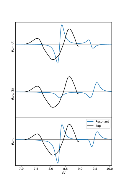
Figure 1: Cyclopropane. CCSD relative contributions of ${\mathcal{A}}_{\rm{CC}}$ (upper panel) and ${\mathcal{B}}_{\rm{CC}}$ (mid panel) terms of resonant response theory to the total (lower panel) broadened MCD spectrum. The experimental spectrum was taken from Ref. 40.

Based on the values in Table 1, Figure 1 illustrates the relative importance of the ${\mathcal{A}}$ and ${\mathcal{B}}$ terms. Clearly, the bisignate spectral feature centered at 8.30 eV is dominated by the positive ${\mathcal{A}}$ term contribution of the second E^′ excited state, where the ${\mathcal{B}}$ term is causing the slightly asymmetry of the dispersion band. The second bisignate feature at around 9.5 eV is the result of the fine balance of the negative ${\mathcal{A}}$ term for the third E^′ state and the oppositely signed pseudo ${\mathcal{A}}$ due to the ${\mathcal{B}}$ terms of the close-lying third E^′ state and the non-degenerate A${}^{\prime\prime}_{2}$ state.

The total MCD spectrum generated by Lorentzian broadening of the ${\mathcal{A}}$ and ${\mathcal{B}}$ terms is compared with the spectrum obtained directly from damped response theory in Figure 2. The broadened spectrum is basically identical to the one of damped response theory. The CAM-B3LYP spectrum is red-shifted compared to the CCSD one, and with slightly weaker intensities, but otherwise the spectral profiles are similar.

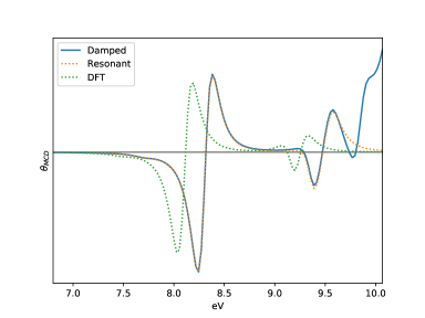
Figure 2: Cyclopropane. CCSD/aug-cc-pVDZ MCD spectra from damped and resonant response theory, and comparison with the CAM-B3LYP spectrum from resonant response theory.

Table 2 collects the values of the excitation energies and MCD spectral parameters for urea, as obtained from resonant response theory. Only ${\mathcal{B}}$ terms are possible by symmetry. The corresponding MCD spectra, including the ones obtained from damped response, are shown in Figure 3. Also in this case, damped and resonant theories yield almost identical spectra up to the number of frequencies that have been considered. The CAM-B3LYP spectrum is qualitatively very similar, yet with larger intensities from the two excited states at around 8 eV.

Table 2: Urea. Computed spectral parameters: excitation energies ($\omega_{f}$), oscillator strengths (f) and and MCD $\mathcal{B}$ terms. Basis set aug-cc-pVDZ.

CCSD		CAM-B3LYP
$\omega_{f}$/eV (f)	${\mathcal{B}}$/a.u.	$\omega_{f}$/eV (f)	${\mathcal{B}}$/a.u.
6.420 (0.031)	$-$4.78769	6.354 (0.025)	$-$4.91873
6.754 (0.033)	5.23536	6.612 (0.033)	5.66315
7.524 (0.009)	$-$0.67620	7.371 (0.012)	$-$0.62543
7.623 (0.036)	$-$7.46470	7.463 (0.021)	$-$7.63975
7.731 (0.014)	1.53604	7.587 (0.020)	1.83269
7.832 (0.002)	5.05075	7.674 (0.009)	4.95339
8.019 (0.14)	84.0208	7.928 (0.18)	80.3061
8.054 (0.20)	$-$84.0705	8.010 (0.13)	$-$80.2552
8.634 (0.059)	$-$4.23649	8.518 (0.07)	$-$4.09754
8.671 (0.003)	3.05857	8.557 (0.004)	3.01059

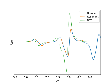
Figure 3: Urea. CCSD/aug-cc-pVDZ MCD spectrum from damped and resonant response theory, and comparison with the CAM-B3LYP one from resonant response theory.

IV Conclusions

We have presented a computational approach to obtain the ${\mathcal{A}}$ term of MCD within CC (resonant) response theory, together with alternative computational recipes for the ${\mathcal{B}}$ term, Moreover, we have derived the computational expression of the MCD ellipticity (temperature-independent part) within CC damped response theory. The latter can prove particularly convenient when the system under investigation is characterized by a large density of excited states. Illustrative results have been reported for cyclopropane and urea, and compared with results from a previous B3LYP implementation of the ${\mathcal{A}}$ and ${\mathcal{B}}$ terms. The spectral profiles were found qualitatively similar, though with noticeable differences on the intensity scale and the usual shifts in the position of the excited states.

Data availability

The data that support the findings of this study are available from the corresponding author upon reasonable request.

V Appendix: The residues of the derivative of the damped CC linear response function

For the analysis of the residues of the derivative of $\langle\langle\mu_{\alpha};\mu_{\beta}\rangle\rangle_{\omega+i\varpi}$ with respect to $B_{\gamma}$ we define the non-phase-isolated derivatives of the eigenvectors with respect to the electric fields:

$$R^{\mu_{\alpha}}_{f}(-\omega) =-\big{(}\mathbf{A}-(\omega_{f}-\omega)\mathbf{1}\big{)}^{-1}\big{(}\mathbf{A}^{\mu_{\alpha}}+\mathbf{B}t^{\mu_{\alpha}}(\omega)\big{)}R_{f}$$ (54)

Of the amplitude and Lagrange multiplier vectors in Eq. (48) only the vectors $t^{\mu_{\beta}}(\omega)$, $\bar{t}^{\mu_{\beta}}(\omega)$, and $\bar{t}^{\mu_{\alpha}}(-\omega)$ have nonvanishing residues in the limit $\omega\to\omega_{f}$:

$$\lim_{\omega\to\omega_{f}}(\omega-\omega_{f})t^{\mu_{\beta}}(\omega) =\sum_{f^{\prime}\in\mathfrak{D}_{f}}R_{f^{\prime}}T^{\mu_{\beta}}_{f^{\prime}0}$$ (55)

$$\lim_{\omega\to\omega_{f}}(\omega-\omega_{f})\bar{t}^{\mu_{\beta}}(\omega) =\sum_{f^{\prime}\in\mathfrak{D}_{f}}T^{\mu_{\beta}}_{f^{\prime}0}\cdot M_{f^{\prime}}$$ (56)

$$\lim_{\omega\to\omega_{f}}(\omega-\omega_{f})\bar{t}^{\mu_{\alpha}}(-\omega) =\sum_{f^{\prime}\in\mathfrak{D}_{f}}T^{\mu_{\alpha}}_{0f^{\prime}}\cdot L_{f^{\prime}}$$ (57)

We get for the non-singular part of residue (simple pole) for the limit $\omega\to\omega_{f}$:

$$\lim_{\omega+i\varpi\to\omega_{f}}(\omega+i\varpi-\omega_{f})\frac{d\langle\!\langle\mu_{\alpha};\mu_{\beta}\rangle\!\rangle_{\omega+i\varpi}}{d\epsilon_{\gamma}}\bigg{|}_{\text{non-res}}$$

$$= \frac{1}{2}\mathcal{P}^{\alpha\beta}\sum_{f^{\prime}\in\mathfrak{D}_{f}}\bigg{\{}\big{(}\mathbf{F}^{m_{\gamma}}t^{\mu_{\alpha}}(-\omega_{f})R_{f^{\prime}}\big{)}\cdot T^{\mu_{\beta}}_{f^{\prime}0}$$ (58)

$$+\Big{(}\Big{[}\mathbf{F}^{\mu_{\alpha}}+\mathbf{G}t^{\mu_{\alpha}}(-\omega_{f})\Big{]}{R}_{f^{\prime}}t^{m_{\gamma}}\Big{)}\cdot T^{\mu_{\beta}}_{f^{\prime}0}$$

$$+\Big{(}\bar{t}^{m_{\gamma}}\Big{[}\mathbf{A}^{\mu_{\alpha}}+\mathbf{B}t^{\mu_{\alpha}}(-\omega_{f})\Big{]}{R}_{f^{\prime}}\Big{)}\cdot T^{\mu_{\beta}}_{f^{\prime}0}$$

$$+\Big{(}{{}^{\perp}\bar{t}}^{\mu_{\alpha}}(-\omega_{f})\Big{[}\mathbf{A}^{m_{\gamma}}+\mathbf{B}t^{m_{\gamma}}\Big{]}{R}_{f^{\prime}}\Big{)}\cdot T^{\mu_{\beta}}_{f^{\prime}0}$$

$$+L_{f^{\prime}}\Big{[}\mathbf{A}^{\mu_{\beta}}t^{m_{\gamma}}+\mathbf{A}^{m_{\gamma}}{{}^{\perp}t}^{\mu_{\beta}}(\omega_{f})+\mathbf{B}t^{m_{\gamma}}{{}^{\perp}t}^{\mu_{\beta}}(\omega_{f})\Big{]}\cdot T^{\mu_{\alpha}}_{0f^{\prime}}$$

$$+M_{f^{\prime}}\Big{[}\mathbf{A}^{\mu_{\alpha}}t^{m_{\gamma}}+\mathbf{A}^{m_{\gamma}}t^{\mu_{\alpha}}(-\omega_{f})+\mathbf{B}t^{m_{\gamma}}t^{\mu_{\alpha}}(-\omega_{f})\Big{]}\cdot T^{\mu_{\beta}}_{f^{\prime}0}\bigg{\}}$$

$$= \frac{1}{2}\mathcal{P}^{\alpha\beta}\sum_{f^{\prime}\in\mathfrak{D}_{f}}\bigg{\{}\Big{(}\bar{\xi}^{m_{\gamma}}R^{\mu_{\alpha}}_{f^{\prime}}(-\omega_{f})\Big{)}\cdot T^{\mu_{\beta}}_{f^{\prime}0}$$ (59)

$$+\Big{(}\bar{\xi}^{\mu_{\alpha}}(-\omega_{f}){{}^{\perp}R}_{f^{\prime}}^{m_{\gamma}}\Big{)}\cdot T^{\mu_{\beta}}_{f^{\prime}0}$$

$$+\Big{(}\Big{[}\mathbf{F}^{m_{\gamma}}t^{\mu_{\alpha}}(-\omega_{f})+\mathbf{F}^{\mu_{\alpha}}t^{m_{\gamma}}+\mathbf{G}t^{\mu_{\alpha}}(-\omega_{f})t^{m_{\gamma}}\Big{]}R_{f^{\prime}}\Big{)}\cdot T^{\mu_{\beta}}_{f^{\prime}0}$$

$$+M_{f^{\prime}}\Big{[}\mathbf{A}^{\mu_{\alpha}}t^{m_{\gamma}}+\mathbf{A}^{m_{\gamma}}t^{\mu_{\alpha}}(-\omega_{f})+\mathbf{B}t^{m_{\gamma}}t^{\mu_{\alpha}}(-\omega_{f})\Big{]}\cdot T^{\mu_{\beta}}_{f^{\prime}0}$$

$$+T^{\mu_{\alpha}}_{0f^{\prime}}\cdot\Big{(}L_{f^{\prime}}\mathbf{A}^{\mu_{\beta}}t^{m_{\gamma}}+{{}^{\perp}L}^{m_{\gamma}}_{f^{\prime}}\xi^{\mu_{\beta}}\Big{)}\bigg{\}}$$

$$= \frac{1}{2}\mathcal{P}^{\alpha\beta}\sum_{f^{\prime}\in\mathfrak{D}_{f}}\bigg{\{}\frac{dT^{\mu_{\alpha}}_{0f^{\prime}}}{d\epsilon_{\gamma}}T^{\mu_{\beta}}_{f^{\prime}0}+T^{\mu_{\alpha}}_{0f^{\prime}}\cdot\frac{dT^{\mu_{\beta}}_{f^{\prime}0}}{d\epsilon_{\gamma}}\bigg{\}}$$ (60)

Only one contribution to the derivative of the damped linear response function, $\bar{t}^{\mu_{\alpha}}(-\omega-i\varpi)\big{[}\mathbf{A}^{m_{\gamma}}+\mathbf{B}t^{m_{\gamma}}]t^{\mu_{\beta}}(\omega+i\varpi)$, contains two vectors that become singular for $\omega\to\omega_{f}$ and contributes to the second-order residue:

$$\lim_{\omega+i\varpi\to\omega_{f}} (\omega+i\varpi-\omega_{f})^{2}\frac{d\langle\!\langle\mu_{\alpha};\mu_{\beta}\rangle\!\rangle_{\omega+i\varpi}}{d\epsilon_{\gamma}}$$ (61)

$$=\frac{1}{2}\mathcal{P}^{\alpha\beta}\sum_{{f,f^{\prime}\in\mathfrak{D}_{f}}}T^{\mu_{\alpha}}_{0f^{\prime}}\cdot\Big{(}L_{f^{\prime}}\Big{[}\mathbf{A}^{m_{\gamma}}+\mathbf{B}t^{m_{\gamma}}\Big{]}R_{f}\Big{)}T^{\mu_{\beta}}_{f0}$$

$$=\mathcal{P}^{\alpha\beta}\sum_{f<f^{\prime}\in\mathfrak{D}_{f}}T^{\mu_{\alpha}}_{0f^{\prime}}\cdot T^{m_{\gamma}}_{f^{\prime}f}\cdot T^{\mu_{\beta}}_{f0}$$ (62)

If we include the Levi-Civita tensor and the negative sign from Eq. (45), the results agree with definition of the $\mathcal{B}$ and $\mathcal{A}$ terms in Eqs. (28) and (42).

References

• Mason (2007) W. R. Mason, A Practical Guide to Magnetic Circular Dichroism Spectroscopy (Wiley, New York, 2007).
• Buckingham and Stephens (1966) A. Buckingham and P. Stephens, “Magnetic optical activity,” Ann. Rev. Phys. Chem. 17, 399 (1966).
• Michl (1976) J. Michl, “Use of semi-empirical models for calculation of b terms in mcd spectra. aromatic hydrocarbons: prediction of substituent and heteroatom effects from ppp model,” Chem. Phys. Lett. 39, 386–390 (1976).
• Castellan and Michl (1978) A. Castellan and J. Michl, “Magnetic Circular Dichroism of Cyclic $\pi$-Electron Systems. Aza Analogues of Benzene,”  100, 6824 (1978).
• Meier (1987) G. Meier, A. A.; Wagnière, “The long-wavelength mcd of some quinones and its interpretation by semi-empirical mo methods,” Chem. Phys. 113, 287–307 (1987).
• Kjærgaard, Coriani, and Ruud (2012) T. Kjærgaard, S. Coriani,  and K. Ruud, “Ab initio calculation of magnetic circular dichroism,” WIREs Computational Molecular Science 2, 443–455 (2012).
• Olsen and Jørgensen (1985) J. Olsen and P. Jørgensen, “Linear and nonlinear response functions for an exact state and for an mcscf state,” J. Chem. Phys. 82, 3235 (1985).
• Helgaker et al. (2012) T. Helgaker, S. Coriani, P. Jørgensen, K. Kristensen, J. Olsen,  and K. Ruud, “Recent advances in wave function-based methods of molecular-property calculations,” Chem. Rev. 112, 543–631 (2012).
• Norman (2011) P. Norman, “A perspective on non resonant and resonant electronic response theory for time-dependent molecular properties,”  12, 20519–20535 (2011).
• Coriani et al. (1999) S. Coriani, P. Jørgensen, K. Ruud, A. Rizzo,  and J. Olsen, “Ab Initio Determinations of Magnetic Circular Dichroism,” Chem. Phys. Lett. 300, 61–68 (1999).
• Solheim et al. (2008a) H. Solheim, K. Ruud, S. Coriani,  and P. Norman, “Complex Polarization Propagator Calculations of Magnetic Circular Dichroism Spectra.” J. Chem. Phys. 128, 094103 (2008a).
• Seth et al. (2008a) M. Seth, M. Krykunov, T. Ziegler,  and J. Autschbach, “Application of Magnetically Perturbed Time-Dependent Density Functional Theory to Magnetic Circular Dichroism. II. Calculation of ${\mathcal{A}}$ Terms,” J. Chem. Phys. 128, 234102 (2008a).
• Kjærgaard et al. (2011) T. Kjærgaard, K. Kristensen, J. Kauczor, P. Jørgensen, S. Coriani,  and A. J. Thorvaldsen, “Comparison of standard and damped response formulations of magnetic circular dichroism,” J. Chem. Phys. 135, 024112 (2011).
• Seth et al. (2008b) M. Seth, M. Krykunov, T. Ziegler, J. Autschbach,  and A. Banerjee, “Application of Magnetically Perturbed Time-Dependent Density Functional Theory to Magnetic Circular Dichroism: Calculation of ${\mathcal{B}}$ Terms,” J. Chem. Phys. 128, 144105 (2008b).
• Solheim et al. (2008b) H. Solheim, K. Ruud, S. Coriani,  and P. Norman, “The A and B Terms of Magnetic Circular Dichroism Revisited,” J. Phys. Chem. A 112, 9615–9618 (2008b).
• Stepanek and Bour (2013) P. Stepanek and P. Bour, “Computation of magnetic circular dichroism by sum-over-states summations,” J. Comput. Chem. 34, 1531–1539 (2013).
• Honda et al. (2005) Y. Honda, M. Hada, M. Ehara, H. Nakatsuji,  and J. Michl, “Theoretical Studies on Magnetic Circular Dichroism by the Finite Perturbation Method with Relativistic Corrections,” J. Chem. Phys. 123, 164113 (2005).
• Ganyushin and Neese (2008) D. Ganyushin and F. Neese, “First-Principles Calculations of Magnetic Circular Dichroism Spectra,” J. Chem. Phys. 128, 114117 (2008).
• Heit, Sergentu, and Autschbach (2019) Y. N. Heit, D.-C. Sergentu,  and J. Autschbach, “Magnetic circular dichroism spectra of transition metal complexes calculated from restricted active space wavefunctions,” Phys. Chem. Chem. Phys. 21, 5586–5597 (2019).
• Krykunov et al. (2007) M. Krykunov, M. Seth, T. Ziegler,  and J. Autschbach, “Calculation of the Magnetic Circular Dichroism B Term from the Imaginary Part of the Verdet Constant using Damped Time-Dependent Density Functional Theory,” J. Chem. Phys. 127, 244102 (2007).
• Kjærgaard et al. (2009) T. Kjærgaard, P. Jørgensen, A. Thorvaldsen, P. Sałek,  and S. Coriani, “Gauge-origin Independent Formulation and Implementation of Magneto-Optical Activity within Atomic-Orbital-Density Based Hartree-Fock and Kohn-Sham Response Theories,” J. Chem. Theory Comp. 5, 1997–2020 (2009).
• Coriani et al. (2000) S. Coriani, C. Hättig, P. Jørgensen,  and T. Helgaker, “Gauge-origin independent magneto-optical activity within coupled cluster response theory,” J. Chem. Phys. 113, 3561 (2000).
• Kjærgaard et al. (2007) T. Kjærgaard, B. Jansík, P. Jørgensen, S. Coriani,  and J. Michl, “Gauge-origin-independent Coupled Cluster Singles and Doubles Calculation of Magnetic Circular Dichroism of Azabenzenes and Phosphabenzene using London Orbitals,” J. Phys. Chem. A 111, 11278–11286 (2007).
• Lee, Yabana, and Bertsch (2011) K.-M. Lee, K. Yabana,  and G. F. Bertsch, “Magnetic Circular Dichroism in Real-Time Time-Dependent Density Functional Theory,” J. Chem. Phys. 134, 144106 (2011).
• Sun, Williams-Young, and Li (2019) S. Sun, D. Williams-Young,  and X. Li, “An ab initio linear response method for computing magnetic circular dichroism spectra with nonperturbative treatment of magnetic field,” J. Chem. Theory Comput. 15, 3162–3169 (2019).
• Michl (1978) J. Michl, “Magnetic circular dichroism of cyclic $\pi$-electron systems. 1. Algebraic solution of the perimeter model for the $A$ and $B$ terms of high-symmetry systems with a (4N + 2)-electron [n]annulene perimeter,” J. Am. Chem. Soc. 100, 6801–6811 (1978).
• Barron (2004) L. D. Barron, Molecular light scattering and optical activity (Cambridge University Press, Cambridge, 2004).
• Piepho and Schatz (1983) S. B. Piepho and P. N. Schatz, Group Theory in Spectroscopy with Applications to Magnetic Circular Dichroism (John Wiley and Sons Inc, New York, 1983).
• Christiansen, Jørgensen, and Hättig (1998) O. Christiansen, P. Jørgensen,  and C. Hättig, “Response functions from fourier component variational perturbation theory applied to a time-averaged quasienergy,” Int. J. Quantum Chem. 98, 1 (1998).
• Hättig, Christiansen, and Jørgensen (1998) C. Hättig, O. Christiansen,  and P. Jørgensen, “Multiphoton transition moments and absorption cross sections in coupled cluster response theory employing variational transition moment functionals.” J. Chem. Phys. 108, 8331–8354 (1998).
• Hättig and Jørgensen (1998) C. Hättig and P. Jørgensen, “Derivation of coupled cluster excited states response functions and multiphoton transition moments between two excited states as derivatives of variational functionals,” J. Chem. Phys. 109, 9219 (1998).
• Aidas et al. (2014) K. Aidas, C. Angeli, K. L. Bak, V. Bakken, R. Bast, L. Boman, O. Christiansen, R. Cimiraglia, S. Coriani, P. Dahle, E. K. Dalskov, U. Ekström, T. Enevoldsen, J. J. Eriksen, P. Ettenhuber, B. Fernández, L. Ferrighi, H. Fliegl, L. Frediani, K. Hald, A. Halkier, C. Hättig, H. Heiberg, T. Helgaker, A. C. Hennum, H. Hettema, E. Hjertenæs, S. Høst, I.-M. Høyvik, M. F. Iozzi, B. Jansik, H. J. A. Jensen, D. Jonsson, P. Jørgensen, J. Kauczor, S. Kirpekar, T. Kjærgaard, W. Klopper, S. Knecht, R. Kobayashi, H. Koch, J. Kongsted, A. Krapp, K. Kristensen, A. Ligabue, O. B. Lutnæs, J. I. Melo, K. V. Mikkelsen, R. H. Myhre, C. Neiss, C. B. Nielsen, P. Norman, J. Olsen, J. M. H. Olsen, A. Osted, M. J. Packer, F. Pawlowski, T. B. Pedersen, P. F. Provasi, S. Reine, Z. Rinkevicius, T. A. Ruden, K. Ruud, V. V. Rybkin, P. Salek, C. C. M. Samson, A. S. de Merás, T. Saue, S. P. A. Sauer, B. Schimmelpfennig, K. Sneskov, A. H. Steindal, K. O. Sylvester-Hvid, P. R. Taylor, A. M. Teale, E. I. Tellgren, D. P. Tew, A. J. Thorvaldsen, L. Thøgersen, O. Vahtras, M. A. Watson, D. J. D. Wilson, M. Ziolkowski,  and H. Ågren, “The Dalton quantum chemistry program system,” WIREs Computational Molecular Science 4, 269 (2014).
• Khani et al. (2019) S. K. Khani, R. Faber, F. Santoro, C. Hättig,  and S. Coriani, “Uv absorption and magnetic circular dichroism spectra of purine, adenine, and guanine: A coupled cluster study in vacuo and in aqueous solution,” J. Chem. Theory Comput. 15, 1242–1254 (2019).
• Furche et al. (2014) F. Furche, R. Ahlrichs, C. Hättig, W. Klopper, M. Sierka,  and F. Weigend, WIREs Computational Molecular Science 4, 91–100 (2014).
• Kauczor et al. (2013) J. Kauczor, P. Norman, O. Christiansen,  and S. Coriani, “Communication: A reduced-space algorithm for the solution of the complex linear response equations used in coupled cluster damped response theory,” J. Chem. Phys. 139, 211102 (2013).
• Faber and Coriani (2019) R. Faber and S. Coriani, “Resonant inelastic x-ray scattering and nonesonant x-ray emission spectra from coupled-cluster (damped) response theory,” J. Chem. Theory Comput. 15, 520–528 (2019).
• Faber and Coriani (2020) R. Faber and S. Coriani, “Core–valence-separated coupled-cluster-singles-and-doubles complex-polarization-propagator approach to x-ray spectroscopies,” Phys. Chem. Chem. Phys. 22, 2642–2647 (2020).
• Faber (2020) R. Faber, “py-ccrsp, Python module for CC response experiments,”  (2020).
• Goldstein, Vijaya, and Segal (1980) E. Goldstein, S. Vijaya,  and G. A. Segal, “Theoretical study of the optical absorption and magnetic circular dichroism spectra of cyclopropane,” J. Am. Chem. Soc. 102, 6198–6204 (1980).
• Gedanken and Schnepp (1976) A. Gedanken and O. Schnepp, “The excited states of cyclopropane. MCD spectrum, and CD spectrum of an optically active derivative,” Chem. Phys. 12, 341–348 (1976).