Continuation methods with the trusty time-stepping scheme for linearly constrained optimization with noisy data

Abstract

The nonlinear optimization problem with linear constraints has many applications in engineering fields such as the visual-inertial navigation and localization of an unmanned aerial vehicle maintaining the horizontal flight. In order to solve this practical problem efficiently, this paper constructs a continuation method with the trusty time-stepping scheme for the linearly equality-constrained optimization problem at every sampling time. At every iteration, the new method only solves a system of linear equations other than the traditional optimization method such as the sequential quadratic programming (SQP) method, which needs to solve a quadratic programming subproblem. Consequently, the new method can save much more computational time than SQP. Numerical results show that the new method works well for this problem and its consumed time is about one fifth of that of SQP (the built-in subroutine fmincon.m of the MATLAB2018a environment) or that of the traditional dynamical method (the built-in subroutine ode15s.m of the MATLAB2018a environment). Furthermore, we also give the global convergence analysis of the new method.

1 Introduction

In this article, we consider the following linearly equality-constrained optimization problem

$$\min_{x\in\Re^{n}}\;f(x)$$

$$\text{subject to}\;\;Ax=b,$$ (1)

where matrix $A\in\Re^{m\times n}$ and vector $b\in\Re^{m}$ may have random noise. This problem has many applications in engineering fields such as the visual-inertial navigation of an unmanned aerial vehicle maintaining the horizontal flight CMFO2009 ; LLS2020 ; ZS2015 , and there are many practical methods to solve it such as the sequential quadratic programming (SQP) method NW1999 or the penalty function method FM1990 .

The penalty function method obtains the solution of the linearly equality-constrained optimization problem (1) via solving the following sequential unconstrained minimization

$$\min_{x\in\Re^{n}}\;P_{\sigma}(x)=f(x)+\sigma\|Ax-b\|^{2},$$ (2)

with increasing $\sigma$. If we denote the global optimal solution of the unconstrained optimization problem (2) as $x_{\sigma}^{\ast}$, it is well known that

$$\lim_{\sigma\to\infty}\;x_{\sigma}^{\ast}=x^{\ast},$$

where $x^{\ast}$ is the optimal solution of the original constrained optimization problem (1) FM1990 . The penalty function method has the asymptotic convergence as $\sigma\to\infty$ for the constrained optimization problem (1). However, in practice, it will meet the ill conditioning which depends on the ratio of the largest to the smallest eigenvalue (the condition number) of the Hessian matrix $\nabla_{xx}^{2}P_{\sigma}(x_{\sigma}^{\ast})$, and this ratio tends to increase with $\sigma$ (pp. 475-476, Bertsekas2018 ). It can be roughly shown as follows.

We denote the rank of matrix $A$ as $r$ and assume that $r<\min\{m,\,n\}$. From problem (2), we obtain the Hessian matrix $H_{\sigma}(x)$ of $P_{\sigma}(x)$ via the simple calculation as follows:

$$H_{\sigma}(x)=\nabla_{xx}^{2}P_{\sigma}(x)=\nabla^{2}f(x)+2\sigma A^{T}A.$$ (3)

We define $\mu_{i}(B)\,(i=1,\,2,\ldots,\,n)$ as the eigenvalues of matrix $B\in\Re^{n\times n}$. $\mu_{min}(B)$ and $\mu_{max}(B)$ represent the smallest and largest eigenvalues of matrix $B$, respectively. From the Courant-Fisher minimax theorem (p. 441, GV2013 ) and equation (3), we have

$$\mu_{min}\left(\nabla^{2}f(x)\right)\leq\mu_{min}(H_{\sigma}(x))=\min_{\|y\|=1}y^{T}H_{\sigma}(x)y\leq\min_{\|y\|=1,\;Ay=0}y^{T}H_{\sigma}(x)y$$

$$\quad=\min_{\|y\|=1,\;Ay=0}y^{T}\nabla^{2}f(x)y\leq\mu_{max}\left(\nabla^{2}f(x)\right)\leq\max_{i=1,\,2,\,\ldots,\,n}\left|\mu_{i}\left(\nabla^{2}f(x)\right)\right|\triangleq M(x).$$ (4)

By combining $\mu_{min}\left(\nabla^{2}f(x)\right)\geq-M(x)$ with equation (4), we have

$$\min_{1\leq i\leq n}\left|\mu_{i}(H_{\sigma}(x))\right|\leq\left|\mu_{min}(H_{\sigma}(x))\right|\leq M(x).$$ (5)

Similarly, from equation (3), we have

$$\mu_{max}(H_{\sigma}(x))=\max_{\|y\|=1}y^{T}H_{\sigma}(x)y=\max_{\|y\|=1}\left(\sigma y^{T}A^{T}Ay+y^{T}\nabla^{2}f(x)y\right)$$

$$\quad\geq\max_{\|y\|=1}\left(\sigma y^{T}A^{T}Ay+\min_{\|y\|=1}y^{T}\nabla^{2}f(x)y\right)=\max_{\|y\|=1}\sigma y^{T}A^{T}Ay+\min_{\|y\|=1}y^{T}\nabla^{2}f(x)y$$

$$\quad=\sigma\mu_{max}\left(A^{T}A\right)+\min_{\|y\|=1}y^{T}\nabla^{2}f(x)y=\sigma\mu_{max}\left(A^{T}A\right)+\mu_{min}\left(\nabla^{2}f(x)\right).$$ (6)

From equations (5)-(6), we obtain

$$\lim_{\sigma\to\infty}\frac{\mu_{max}(H_{\sigma}(x))}{\min_{1\leq i\leq n}|\mu_{i}(H_{\sigma}(x))|}\geq\lim_{\sigma\to\infty}\frac{\sigma\mu_{max}(A^{T}A)+\mu_{min}\left(\nabla^{2}f(x)\right)}{M(x)}=\infty.$$ (7)

That is to say, the condition number of the Hessian matrix $H_{\sigma}(x)$ tends to infinity.

In order to overcome the numerical difficulty of the penalty function method near the optimal point $x^{\ast}$ of the constrained optimization problem (1), there are some promising methods such as the dynamical methods AG2003 ; CKK2003 ; Goh2011 ; KLQCRW2008 ; Tanabe1980 or the SQP methods Bertsekas2018 ; Heinken1996 ; NW1999 for this problem via handling its first-order Karush-Kuhn-Tucker conditions directly. The advantage of the dynamical method over the SQP method is that the dynamical method is capable of finding many local optimal points of non-convex optimization problems by tracking the trajectories, and it is even possible to find the global optimal solution BB1989 ; Schropp2000 ; Yamashita1980 . However, the dynamical method requires more iteration steps and consumes more time than SQP. In order to improve the computational efficiency of the dynamical method, we consider a continuation method with the new time-stepping scheme based on the trust-region technique in this article.

The rest of the paper is organized as follows. In section 2, we construct a new continuation method with the trusty time-stepping scheme for the linearly equality-constrained optimization problem (1). In section 3, we give the global convergence analysis of this new method. In section 4, we report some promising numerical results of the new method, in comparison to the traditional SQP method and the traditional dynamical method for some large scale test problems and a real-world optimization problem which arises from the visual-inertial navigation and localization problem with or without the random errors. Finally, we give some discussions and conclusions in section 5.

2 Continuation Methods with the Trusty Time-stepping Scheme

In this section, we construct a continuation method with the new time-stepping scheme based on the trust-region technique Yuan2015 for the linearly equality-constrained optimization problem (1) via following the trajectory of the differential-algebraic dynamical system to obtain its equilibrium point.

2.1 The Differential-Algebraic Dynamical System

For the linearly constrained optimization problem (1), it is well known that its optimal solution $x^{\ast}$ needs to satisfy the Karush-Kuhn-Tucker conditions (p. 328, NW1999 ) as follows:

$$\nabla_{x}L(x,\lambda) =\nabla f(x)+A^{T}\lambda=0,$$ (8)

$$Ax-b =0,$$ (9)

where the Lagrangian function $L(x,\lambda)$ is defined by

$$L(x,\;\lambda)=f(x)+\lambda^{T}(Ax-b).$$ (10)

Similarly to the method of the negative gradient flow for the unconstrained optimization problem LKLT2009 , from the first-order necessary conditions (8)-(9), we can construct a dynamical system of differential-algebraic equations for problem (1) LL2010 ; Luo2012 ; LLW2013 ; Schropp2003 as follows:

$$\frac{dx}{dt}=-\nabla L_{x}(x,\lambda)=-\left(\nabla f(x)+A^{T}\lambda\right),$$ (11)

$$Ax-b=0.$$ (12)

By differentiating the algebraic constraint (12) with respect to $t$ and replacing it into the differential equation (11), we obtain

$$A\frac{dx}{dt}=-A\left(\nabla f(x)+A^{T}\lambda\right)=-A\nabla f(x)-AA^{T}\lambda=0.$$ (13)

If we assume that matrix $A$ has full row rank further, from equation (13), we obtain

$$\lambda=-\left(AA^{T}\right)^{-1}A\nabla f(x).$$ (14)

By replacing $\lambda$ of equation (14) into equation (11), we obtain the dynamical system of ordinary differential equations (ODEs) as follows:

$$\frac{dx}{dt}=-\left(I-A^{T}\left(AA^{T}\right)^{-1}A\right)\nabla f(x).$$ (15)

Thus, we also obtain the projection gradient flow for the constrained optimization problem Tanabe1980 .

For convenience, we denote the projection matrix $P$ as

$$P=I-A^{T}\left(AA^{T}\right)^{-1}A.$$ (16)

It is not difficult to verify $P^{2}=P$ and $PA^{T}=0$. That is to say, $P$ is a symmetric projection matrix and its eigenvalues are 0 or 1. From Theorem 2.3.1 in p. 73 of GV2013 , we know that its matrix 2-norm is

$$\|P\|=1.$$ (17)

Remark 1

If $x(t)$ is the solution of ODEs (15), it is not difficult to verify that $x(t)$ satisfies $A(dx/dt)=0$. That is to say, if the initial point $x_{0}$ of ODEs (15) satisfies $Ax_{0}=b$, the solution $x(t)$ of ODEs (15) also satisfies $Ax(t)=b,\;\forall t\geq 0$.

Remark 2

If we assume that $x(t)$ is the solution of ODEs (15), from equations (16)-(17), we obtain

$$\frac{df(x)}{dt} =\left(\nabla f(x)\right)^{T}\frac{dx}{dt}=-(\nabla f(x))^{T}P\nabla f(x)=-(\nabla f(x))^{T}P^{2}\nabla f(x)$$

$$=-(P\nabla f(x))^{T}(P\nabla f(x))=-\|P\nabla f(x)\|_{2}^{2}\leq 0.$$

That is to say, $f(x)$ is monotonically decreasing along the solution curve $x(t)$ of the dynamical system (15). Furthermore, the solution $x(t)$ converges to $x^{\ast}$ when $t$ tends to infinity Schropp2000 ; Tanabe1980 , where $x^{\ast}$ satisfies the first-order Karush-Kuhn-Tucker conditions (8)-(9). Thus, we can follow the trajectory $x(t)$ of the ordinary differential equation (15) or the trajectory $(x(t),\,\lambda(t))$ of differential-algebraic equations (11)-(12) to obtain their equilibrium point $x^{\ast}$, which is also one saddle point of the original optimization problem (1).

2.2 Continuation Methods

The solution curve of general differential-algebraic equations is not efficiently followed on an infinite interval by the traditional ODE method AP1998 ; BCP1996 ; HW1996 ; LF2000 , so one needs to construct the particular method for this problem (11)-(12). We regard the algebraic equation (12) as a degenerate differential equation BCP1996 ; CKK2003 ; Shampine2002 , and apply the first-order implicit Euler method to the system of differential-algebraic equations (11)-(12), then we obtain

$$x_{k+1}=x_{k}-\Delta t_{k}\left(\nabla f(x_{k+1})+A^{T}\lambda_{k+1}\right),$$ (18)

$$Ax_{k+1}-b=0,$$ (19)

where $\Delta t_{k}$ is the time-stepping size.

Since the system of equations (18)-(19) is a nonlinear system which is not directly solved, we seek for its explicit approximation formula. We denote $s_{k}=x_{k+1}-x_{k}$. By using the first-order Taylor expansion, we have the linear approximation $\nabla f(x_{k})+\nabla^{2}f(x_{k})s_{k}$ of $\nabla f(x_{k+1})$. From equation (14) and the first-order Taylor expansion, we have

$$\lambda_{k+1} =-(AA^{T})^{-1}A\nabla f(x_{k+1})\approx-(AA^{T})^{-1}A\nabla f(x_{k})-(AA^{T})^{-1}A\nabla^{2}f(x_{k})s_{k}$$

$$=\lambda_{k}-(AA^{T})^{-1}A\nabla^{2}f(x_{k})s_{k}.$$

By replacing them into equation (18), we obtain the predictor $x_{k+1}^{P}$ of $x_{k+1}$ as follows:

$$\left({1}/{\Delta t_{k}}I+B_{k}\right)d_{k} =-p_{g_{k}},$$ (20)

$$x_{k+1}^{P} =x_{k}+d_{k},$$ (21)

where $B_{k}$ equals the Jacobian matrix $\nabla^{2}f(x_{k})+A^{T}\frac{\partial}{\partial x}\lambda(x_{k})$ ($\lambda(x)$ defined by equation (14)) or its quasi-Newton approximation matrix, and

$$p_{g_{k}}=\nabla_{x}L(x_{k},\;\lambda_{k})=\nabla f(x_{k})+A^{T}\lambda_{k}.$$ (22)

The predicted point $x_{k+1}^{P}$ will escape from the constraint plane (12), so we pull it back to the constraint plane by solving the following projection problem:

$$\min_{x\in\Re^{n}}\;\left\|x-x_{k+1}^{P}\right\|^{2}\;\text{subject to}\hskip 5.69054ptAx=b.$$ (23)

It is not difficult to obtain the solution of the linearly constrained least-squares problem (23) via using the Lagrangian multiplier method (p. 479, Bertsekas2018 ) as follows:

$$x_{k+1}=x_{k+1}^{P}+A^{T}\left(AA^{T}\right)^{-1}\left(b-Ax_{k+1}^{P}\right).$$ (24)

Notice that $x_{k+1}$ satisfies the constraint $Ax=b$. From equation (21) and equation (24), we have

$$x_{k+1} =x_{k+1}^{P}+A^{T}\left(AA^{T}\right)^{-1}\left(b-Ax_{k+1}^{P}\right)=x_{k}+d_{k}+A^{T}\left(AA^{T}\right)^{-1}\left(Ax_{k}-Ax_{k+1}^{P}\right)$$

$$=x_{k}+d_{k}-A^{T}\left(AA^{T}\right)^{-1}Ad_{k}=x_{k}+\left(I-A^{T}\left(AA^{T}\right)^{-1}A\right)d_{k}$$

$$=x_{k}+Pd_{k},$$ (25)

where the projection matrix $P$ is defined by equation (16).

After solving $x_{k+1}$ from equation (20) and equation (25), according to equation (14), we obtain the Lagrangian multiplier $\lambda_{k+1}$ as follows:

$$\lambda_{k+1}=-\left(AA^{T}\right)^{-1}A\nabla f(x_{k+1}).$$ (26)

By replacing $\lambda_{k+1}$ of equation (26) into equation (22), we also obtain

$$p_{g_{k}}=\nabla_{x}L(x_{k},\;\lambda_{k})=\nabla f(x_{k})+A^{T}\lambda_{k}=\left(I-A^{T}\left(AA^{T}\right)^{-1}A\right)\nabla f(x_{k})=Pg_{k},$$ (27)

where $g_{k}=\nabla f(x_{k})$ and the projection matrix $P$ is defined by equation (16).

2.3 The Trusty Time-stepping Scheme

Another issue is how to adaptively adjust the time-stepping size $\Delta t_{k}$ at every iteration. We borrow the adjustment method of the trust-region radius from the trust-region method due to its robust convergence and fast local convergence CGT2000 . Since $x_{k+1}$ is the solution of the linearly constrained least-squares problem (23), $x_{k+1}$ maintains the feasibility. Therefore, we use the objective function $f(x)$ instead of the nonsmooth penalty function $f(x)+\sigma\|Ax-b\|_{1}$ as the cost function.

When we use the trust-region technique to adaptively adjust time-stepping size $\Delta t_{k}$ Higham1999 , we also need to construct a local approximation model of the objective $f(x)$ around $x_{k}$. Here, we adopt the following quadratic function as its approximation model:

$$q_{k}(x)=f(x_{k})+(x-x_{k})^{T}g_{k}+{1}/{2}(x-x_{k})^{T}B_{k}(x-x_{k}).$$ (28)

where $g_{k}=\nabla f(x_{k})$ and the symmetric matrix $B_{k}$ equals $\nabla^{2}f(x_{k})+A^{T}\frac{\partial}{\partial x}\lambda(x_{k})$ ($\lambda$ defined by equation (14)) or its quasi-Newton approximation matrix. We enlarge or reduce the time-stepping size $\Delta t_{k}$ at every iteration according to the following ratio:

$$\rho_{k}=\frac{f(x_{k})-f(x_{k+1})}{q_{k}(x_{k})-q_{k}(x_{k+1})}.$$ (29)

A particular adjustment strategy is given as follows:

$$\Delta t_{k+1}=\begin{cases}\gamma_{1}\Delta t_{k},&{if\hskip 2.84526pt0\leq\left|1-\rho_{k}\right|\leq\eta_{1},}\\ \Delta t_{k},&{if\hskip 2.84526pt\eta_{1}<\left|1-\rho_{k}\right|<\eta_{2},}\\ \gamma_{2}\Delta t_{k},&{if\hskip 2.84526pt\left|1-\rho_{k}\right|\geq\eta_{2},}\end{cases}$$ (30)

where the constants are selected as $\eta_{1}=0.25,\;\gamma_{1}=2,\;\eta_{2}=0.75,\;\gamma_{2}=0.5$ according to numerical experiments.

2.4 The Treatments of Deficient Rank and Infeasible Initial Points

For a real-world problem, the rank of matrix $A$ may be deficient and even the constraint system may be inconsistent when the data ($A,\,b$) have random noise. We handle this problem via solving the following best approximation problem

$$\min_{x\in\Re^{n}}\;\|Ax-b\|^{2}$$ (31)

to obtain the reduced constraint system of problem (1).

First, we factorize matrix $A$ with its singular value decomposition (pp. 76-80, GV2013 ) as follows:

$$A=U\Sigma V^{T},\;\Sigma=diag(\sigma_{1},\,\sigma_{2},\,\ldots,\,\sigma_{r},0,\,\ldots,\,0),\;\sigma_{1}\geq\sigma_{2}\geq\ldots\geq\sigma_{r}>0,$$ (32)

where $U\in\Re^{m\times m}$ and $V\in\Re^{n\times n}$ are orthogonal matrices, and $r$ is the rank of matrix $A$. Thus, problem (31) equals the following linear least-squares problem

$$\min_{x\in\Re^{n}}\;\|\Sigma V^{T}x-U^{T}b\|^{2},$$ (33)

which leads to the reduced constraint system

$$V_{r}^{T}x=b_{r},$$ (34)

where $V_{r}=V(1:n,1:r)$,   $V_{r}^{T}V_{r}=I$, and $b_{r}=((U^{T}b)(1:r))./diag(\Sigma(1:r,\,1:r))$.

Therefore, when the constraint system of problem (1) is consistent, it equals the following problem

$$\min_{x\in\Re^{n}}\;f(x)\;\text{subject to}\;V_{r}^{T}x=b_{r}.$$ (35)

When the constraint system of problem (1) is inconsistent, problem (35) is the best relaxation approximation of the original optimization problem (1). After this preprocess, we reformulate the projection matrix $P$ defined by equation (16) as follows:

$$P=I-V_{r}V_{r}^{T}.$$ (36)

Consequently, in subsection 2.2, we only need to replace matrix $A$ and vector $b$ with matrix $V_{r}^{T}$ and vector $b_{r}$ respectively, then the continuation method (25) can handle the deficient rank problem.

For a real-world optimization problem (1), we probably meet the infeasible initial point $x_{0}$. That is to say, the initial point can not satisfy the constraint (34). We handle this problem by solving the following projection problem:

$$\min_{x\in\Re^{n}}\;\left\|x-x_{0}\right\|^{2}\;\text{subject to}\hskip 5.69054ptV_{r}^{T}x=b_{r},$$ (37)

where $V_{r}\in\Re^{n\times r}$ satisfies $V_{r}^{T}V_{r}=I$. By using the Lagrangian multiplier method to solve problem (37), we obtain the initial feasible point $x_{0}^{F}$ of problem (35) as follows:

$$x_{0}^{F}=x_{0}+V_{r}\left(b_{r}-V_{r}^{T}x_{0}\right).$$ (38)

For convenience, we set $x_{0}=x_{0}^{F}$ in line 4, Algorithm 1.

2.5 The BFGS Quasi-Newton Updating Method

For the large-scale problem, the numerical estimation of the Hessian matrix $\nabla^{2}f(x_{k})$ consumes much time. In order to overcome this shortcoming, we use the BFGS quasi-Newton formula (pp. 194-198, NW1999 ) to update the approximation $B_{k}$ of $\nabla^{2}f(x_{k})+A^{T}\frac{\partial}{\partial x}\lambda(x_{k})$, where $\lambda(x)$ is defined by equation (14). The BFGS updating formula can be written as

$$B_{k+1}=B_{k}-\frac{B_{k}s_{k}s_{k}^{T}B_{k}}{s_{k}^{T}B_{k}s_{k}}+\frac{y_{k}y_{k}^{T}}{y_{k}^{T}s_{k}},$$ (39)

where $s_{k}=x_{k+1}-x_{k}$ and $y_{k}=\nabla_{x}L(x_{k+1},\,\lambda_{k+1})-\nabla_{x}L(x_{k},\,\lambda_{k})$ ($\nabla_{x}L(x_{k},\,\lambda_{k})$ defined by equation (22)). The initial matrix $B_{0}$ can be simply selected by the identity matrix.

The BFGS updating formula (39) has some nice properties such as the symmetric positive definite property of matrix $B_{k+1}$ if $B_{k}$ is symmetric positive definite and $y_{k}^{T}s_{k}>0$. Its proof can be found in p. 199, NW1999 . For convenience, we state its brief proof as follows.

Since matrix $B_{k}$ is symmetric positive definite, we have its Cholesky factorization $B_{k}=L_{k}L_{k}^{T}$ and denote

$$\alpha_{k}=L_{k}^{T}s_{k},\;\text{and}\;\beta_{k}=L_{k}^{T}z\;\text{for any}\;z\in\Re^{n}.$$

Thus, for any nonzero $z\in\Re^{n}$, from equation (39) and the assumption $y_{k}^{T}s_{k}>0$, we have

$$z^{T}B_{k+1}z=z^{T}B_{k}z-\frac{(z^{T}B_{k}s_{k})^{2}}{s_{k}^{T}B_{k}s_{k}}+\frac{(z^{T}y_{k})^{2}}{y_{k}^{T}s_{k}}=\|\beta_{k}\|^{2}-\frac{(\alpha_{k}^{T}\beta_{k})^{2}}{\|\alpha_{k}\|^{2}}+\frac{(z^{T}y_{k})^{2}}{y_{k}^{T}s_{k}}\geq 0.$$ (40)

In the last inequality of equation (40), we use the Cauchy-Schwartz inequality $\|\alpha_{k}\|\|\beta_{k}\|$ $\geq|\alpha_{k}^{T}\beta_{k}|$. Its equality holds if only if $\beta_{k}=t\alpha_{k}$. In this case, we have $s_{k}=tz$ since $\alpha_{k}=L_{k}^{T}s_{k}=t\beta_{k}=tL_{k}^{T}z$. Thus, we have $(z^{T}y_{k})^{2}/y_{k}^{T}s_{k}=t^{2}>0$, which leads to $z^{T}B_{k+1}z>0$.

According to the above discussions, we give the detailed implementation of the continuation method with the trusty time-stepping scheme for the linearly equality-constrained optimization problem (1) in Algorithm 1.

Algorithm 1 Continuation methods with the trusty time-stepping scheme for the linearly equality-constrained optimization problem (the Ptctr method)

0:    the objective function: $f(x)$; the linear constraint: $Ax=b$; the initial point: $x_{0}$   (optional); the terminated parameter: $\epsilon$   (optional).

0:    the optimal approximation solution $x^{\ast}$.

1:  If the called function does not provide the initial values $x_{0}$ and $\epsilon$, we set $x_{0}=[1,\,1,\,\ldots,\,1]^{T}$ and $\epsilon=10^{-6}$, respectively.

2:  Initialize the parameters: $\eta_{a}=10^{-6},\;\eta_{1}=0.25,\;\gamma_{1}=2,\;\eta_{2}=0.75,\;\gamma_{2}=0.5$.

3:  Factorize matrix $A$ with the singular value decomposition as follows:

$$A=U\Sigma V^{T},\;\Sigma=diag(\sigma_{1},\,\sigma_{2},\,\ldots,\,\sigma_{r},\,0,\,\ldots,\,0),$$

and denote $V_{r}=V(1:n,1:r)$, $b_{r}=((U^{T}b)(1:r))./diag(\Sigma(1:r,\,1:r))$, where $r$ is the rank of matrix $A$.

4:  Compute

$$x_{0}\leftarrow x_{0}+V_{r}\left(b_{r}-V_{r}^{T}x_{0}\right),$$

such that $x_{0}$ satisfies the linear system of constraints $V_{r}^{T}x=b_{r}$.

5:  Set $k=0$ and $B_{0}=I$. Evaluate $f_{0}=f(x_{0})$ and $g_{0}=\nabla f(x_{0})$.

6:  Compute the projection gradient $p_{g_{0}}=g_{0}-V_{r}\left(V_{r}^{T}g_{0}\right)$.

7:  Compute the initial time-stepping size

$$\Delta t_{0}=\min\left\{10^{-2},\;{1}/{\|p_{g_{0}}\|}\right\}.$$

8:  while $\|p_{g_{k}}\|>\epsilon$ do

9:     if $\left(\frac{1}{\Delta t_{k}}I+B_{k}-P^{T}B_{k}P\right)\succ 0$ && $\left(\frac{1}{\Delta t_{k}}I+B_{k}\right)\succ 0$ then

10:        Solve the linear system (20) by the Cholesky factorization to obtain the search direction $d_{k}$, and compute

$$x_{k+1}=x_{k}+Pd_{k}=x_{k}+\left(I-V_{r}V_{r}^{T}\right)d_{k}=x_{k}+d_{k}-V_{r}\left(V_{r}^{T}d_{k}\right).$$

11:        Evaluate $f_{k+1}=f(x_{k+1})$ and compute the ratio $\rho_{k}$ from equations (28)-(29).

12:     else

13:        Let $\rho_{k}=-1$.

14:     end if

15:     if $\rho_{k}\leq\eta_{a}$ then

16:        Set $x_{k+1}=x_{k},\;f_{k+1}=f_{k},\;p_{g_{k+1}}=p_{g_{k}},\;g_{k+1}=g_{k},\;B_{k+1}=B_{k}.$

17:     else

18:        Evaluate $g_{k+1}=\nabla f(x_{k+1})$, and update $B_{k+1}$ by the BFGS formula (39).

19:        Compute the projection gradient

$$p_{g_{k+1}}=Pg_{k+1}=\left(I-V_{r}V_{r}^{T}\right)g_{k+1}=g_{k+1}-V_{r}\left(V_{r}^{T}g_{k+1}\right).$$

20:     end if

21:     Adjust the time-stepping size $\Delta t_{k+1}$ based on the trust-region updating scheme (30).

22:     Set $k\leftarrow k+1$.

23:  end while

3 Algorithm Analysis

In this section, we analyze the global convergence of the continuation method with the trusty time-stepping scheme for the linearly equality-constrained optimization problem (i.e. Algorithm 1). Firstly, we give a lower-bounded estimate of $q_{k}(x_{k})-q_{k}(x_{k+1})$ $(k=1,\,2,\,\ldots)$. This result is similar to that of the trust-region method for the unconstrained optimization problem Powell1975 . For simplicity, we assume that the rank of matrix $A$ is full and the constraint $Ax=b$ is consistent.

Lemma 1

Assume that the quadratic model $q_{k}(x)$ is defined by equation (28) and $d_{k}$ is the solution of equation (20). Furthermore, we suppose that the time-stepping size $\Delta t_{k}$ satisfies

$$\left(1/{\Delta t_{k}}\,I+B_{k}\right)\succ 0\;\text{and}\;\left({1}/{\Delta t_{k}}\,I+B_{k}-P^{T}B_{k}P\right)\succ 0,$$ (41)

where matrix $P$ is defined by equation (36). Then, we have

$$q_{k}(x_{k})-q_{k}(x_{k}+Pd_{k})\geq{1}/{2}\left\|p_{g_{k}}\right\|\min\left\{\left\|Pd_{k}\right\|,\;\|p_{g_{k}}\|/(3\|B_{k}\|)\right\},$$ (42)

where the projection gradient $p_{g_{k}}=Pg_{k}$.

Proof.  Let $\tau_{k}=1/\Delta t_{k}$. From equation (20), we obtain

$$q_{k}(x_{k}) -q_{k}(x_{k}+Pd_{k})=-{1}/{2}\left(d_{k}^{T}P^{T}B_{k}Pd_{k}\right)-(Pg_{k})^{T}d_{k}$$

$$=-{1}/{2}\left(d_{k}^{T}P^{T}B_{k}Pd_{k}\right)+p_{g_{k}}^{T}\left(\tau_{k}I+B_{k}\right)^{-1}p_{g_{k}}$$

$$={1}/{2}\left(p_{g_{k}}^{T}\left(\tau_{k}I+B_{k}\right)^{-1}p_{g_{k}}+d_{k}^{T}\left(-P^{T}B_{k}P+\tau_{k}I+B_{k}\right)d_{k}\right).$$ (43)

We denote $\mu_{min}\left(B_{k}-P^{T}B_{k}P\right)$ as the smallest eigenvalue of matrix $\left(B_{k}-P^{T}B_{k}P\right)$, and set

$$\tau_{lb}=\min\left\{0,\;\mu_{min}\left(B_{k}-P^{T}B_{k}P\right)\right\}.$$ (44)

From equations (41), (43)-(44) and the bound on the eigenvalues of matrix $(\tau_{k}I+B_{k})^{-1}$, we obtain

$$q_{k}(x_{k})-q_{k}(x_{k}+Pd_{k})\geq{1}/{2}\left(p_{g_{k}}^{T}\left(\tau_{k}I+B_{k}\right)^{-1}p_{g_{k}}+\left(\tau_{k}+\tau_{lb}\right)\left\|d_{k}\right\|^{2}\right)$$

$$\quad\geq{1}/{2}\left({\left\|p_{g_{k}}\right\|^{2}}/{\left(\tau_{k}+\left\|B_{k}\right\|\right)}+\left(\tau_{k}+\tau_{lb}\right)\left\|d_{k}\right\|^{2}\right).$$ (45)

In the above second inequality, we use the property $|\mu_{i}(B_{k})|\leq\|B_{k}\|$, where $\mu_{i}(B_{k})$ is an eigenvalue of matrix $B_{k}$.

Now we consider the properties of the function

$$\varphi(\tau)\triangleq\tau\left\|d_{k}\right\|^{2}+{\left\|p_{g_{k}}\right\|^{2}}/\left(\tau-\tau_{lb}+\left\|B_{k}\right\|\right).$$ (46)

It is not difficult to verify that the second-order derivative of $\varphi(\tau)$ is positive when $\left(\tau-\tau_{lb}+\|B_{k}\right\|)>0$ since $\varphi^{{}^{\prime\prime}}(\tau)=2\|p_{g_{k}}\|^{2}/\left(\tau-\tau_{lb}+\|B_{k}\|\right)^{3}\geq 0$. Thus, the function $\varphi(\tau)$ attains its minimum $\varphi(\tau_{min})$ when $\tau_{min}$ satisfies $\varphi^{{}^{\prime}}(\tau_{min})=0$ and $\tau\geq-(-\tau_{lb}+\|B_{k}\|)$. That is to say, we have

$$\varphi(\tau_{min})=2\|p_{g_{k}}\|\|d_{k}\|+\left(\tau_{lb}-\|B_{k}\|\right)\|d_{k}\|^{2},$$ (47)

where

$$\tau_{min}=\|p_{g_{k}}\|/\|d_{k}\|+\tau_{lb}-\|B_{k}\|.$$ (48)

We prove the property (42) when $\tau_{min}\geq 0$ or $\tau_{min}<0$ separately as follows.

(i) When $\left(\|p_{g_{k}}\|/\|d_{k}\|+\left(\tau_{lb}-\|B_{k}\|\right)\right)\geq 0$, from equation (48), we have $\tau_{min}\geq 0$. From the assumption (41) and the definition (44) of $\tau_{lb}$, we have $\tau_{k}\geq-\tau_{lb}$. Thus, from equations (45)–(48), we obtain

$$q_{k}(x_{k})-q_{k}(x_{k}+Pd_{k})\geq{1}/{2}\left((\tau_{k}+\tau_{lb})\|d_{k}\|^{2}+{\|p_{g_{k}}\|^{2}}/\left(\tau_{k}+\|B_{k}\|\right)\right)$$

$$\quad=1/2\varphi(\tau_{k}+\tau_{lb})\geq{1}/{2}\varphi(\tau_{min})$$

$$\quad={1}/{2}\left(\|p_{g_{k}}\|\|d_{k}\|+\left(\|p_{g_{k}}\|\|d_{k}\|+\left(\tau_{lb}-\|B_{k}\|\right)\|d_{k}\|^{2}\right)\right)\geq{1}/{2}\|p_{g_{k}}\|\|d_{k}\|.$$ (49)

(ii) The other case is $\left(\|p_{g_{k}}\|/\|d_{k}\|+\left(\tau_{lb}-\|B_{k}\|\right)\right)<0$. In this case, from equation (48), we have $\tau_{min}<0$. It is not difficult to verify that $\varphi(\tau)$ is monotonically increasing when $\tau\geq 0$ and $\tau_{min}<0$. From the definition (44) of $\tau_{lb}$ and the property (17), we have

$$|\tau_{lb}| \leq\left|\mu_{min}\left(B_{k}-P^{T}B_{k}P\right)\right|\leq\|B_{k}-P^{T}B_{k}P\|\leq\|B_{k}\|+\|P^{T}B_{k}P\|$$

$$\leq\|B_{k}\|+\|P^{T}\|\|B_{k}\|\|P\|=2\|B_{k}\|.$$

By using this property and the monotonicity of $\varphi(\tau)$, from equations (45)-(46), we obtain

$$q_{k}(x_{k})-q_{k}(x_{k}+Pd_{k})\geq{1}/{2}\left((\tau_{k}+\tau_{lb})\|d_{k}\|^{2}+{\|p_{g_{k}}\|^{2}}/\left(\tau_{k}+\|B_{k}\|\right)\right)$$

$$\quad=\frac{1}{2}\varphi(\tau_{k}+\tau_{lb})\geq\frac{1}{2}\varphi(0)=\frac{1}{2(-\tau_{lb}+\|B_{k}\|)}\|p_{g_{k}}\|^{2}\geq\frac{1}{6\|B_{k}\|}\|p_{g_{k}}\|^{2}.$$ (50)

From equations (49)-(50), we get

$$q_{k}(x_{k})-q_{k}(x_{k}+Pd_{k})\geq{1}/{2}\|p_{g_{k}}\|\min\left\{\|d_{k}\|,\;{\|p_{g_{k}}\|}/{(3\|B_{k}\|)}\right\}.$$ (51)

By using the property (17) of matrix $P$, we have

$$\|Pd_{k}\|\leq\|P\|\|d_{k}\|=\|d_{k}\|.$$ (52)

Therefore, from inequalities (51)-(52), we obtain the estimate (42). ∎

In order to prove that $p_{g_{k}}$ converges to zero when $k$ tends to infinity, we need to estimate the lower bound of time-stepping sizes $\Delta t_{k}\,(k=1,\,2,\,\ldots)$ when $\|p_{g_{k}}\|\geq\epsilon_{p_{g}}>0,\;k=1,\,2,\,\ldots$.

Lemma 2

Assume that $f:\;\Re^{n}\rightarrow\Re$ is twice continuously differentiable and the constrained level set

$$S_{f}=\left\{x:\;f(x)\leq f(x_{0}),\;Ax=b\right\}$$ (53)

is bounded. We assume that the Hessian matrix function $\nabla^{2}f(\cdot)$ is Lipschitz continuous. That is to say, it exists a positive constant $L_{c}$ such that

$$\left\|\nabla^{2}f(x)-\nabla^{2}f(y)\right\|\leq L_{c}\|x-y\|,\;\forall x,\,y\in\Re^{n}.$$ (54)

We suppose that the sequence $\{x_{k}\}$ is generated by Algorithm 1 and the quasi-Newton matrices $B_{k}\,(k=1,\,2,\,\ldots)$ are bounded. That is to say, it exists a positive constant $M_{B}$ such that

$$\|B_{k}\|\leq M_{B},\;k=1,\,2,\ldots.$$ (55)

Furthermore, we assume that it exists a positive constant $\epsilon_{p_{g}}$ such that

$$\|p_{g_{k}}\|\geq\epsilon_{p_{g}}>0,\;k=1,\,2,\ldots,$$ (56)

where $p_{g_{k}}=Pg_{k}$,   $g_{k}=\nabla f(x_{k})$, and $P$ is defined by equation (36). Then, it exists a positive constant $\delta_{\Delta t}$ such that

$$\Delta t_{k}\geq\gamma_{2}\delta_{\Delta t}>0,\;k=1,\;2,\dots,$$ (57)

where $\Delta t_{k}$ is adaptively adjusted by the trust-region updating scheme (28)-(30).

Proof.  Since the level set $S_{f}$ is bounded, according to Proposition A.7 in pp. 754-755 of reference Bertsekas2018 , $S_{f}$ is closed. Thus, it exists two positive constants $M_{g}$ and $M_{G}$ such that

$$\|g_{k}\|\leq M_{g},\;\|G_{k}\|\leq M_{G},\;k=1,\;2,\dots,$$ (58)

where $g_{k}=\nabla f(x_{k})$ and $G_{k}=\nabla^{2}f(x_{k})$. From equation (17), we know $\|P\|=1$. By using this property and the assumption (55), we have

$$\left|\mu_{min}\left(B_{k}-P^{T}B_{k}P\right)\right|\leq\left\|B_{k}-P^{T}B_{k}P\right\|$$

$$\quad\leq\|B_{k}\|+\|P^{T}\|\|B_{k}\|\|P\|=2\|B_{k}\|\leq 2M_{B},\;k=1,\,2,\ldots,$$ (59)

where $\mu_{min}(B)$ represents the smallest eigenvalue of matrix $B$. Thus, from equation (59), we obtain

$$\mu_{min}\left({1}/{\Delta t_{k}}I+B_{k}-P^{T}B_{k}P\right)={1}/{\Delta t_{k}}+\mu_{min}\left(B_{k}-P^{T}B_{k}P\right)$$

$$\quad\geq{1}/{\Delta t_{k}}-2M_{B},\;k=1,\,2,\ldots.$$ (60)

Similarly, from the assumption (55), we have

$$\mu_{min}\left({1}/{\Delta t_{k}}I+B_{k}\right)={1}/{\Delta t_{k}}+\mu_{min}\left(B_{k}\right)\geq{1}/{\Delta t_{k}}-M_{B},\;k=1,\,2,\ldots.$$ (61)

Therefore, the positive definite conditions of equation (41) are satisfied when $\Delta t_{k}<1/(2M_{B})\,(k=1,\,2,\ldots)$.

From a second-order Taylor expansion, we have

$$f(x_{k}+Pd_{k})=f(x_{k})+g_{k}^{T}(Pd_{k})+1/2(Pd_{k})^{T}\nabla^{2}f(\tilde{x}_{k})(Pd_{k}),$$ (62)

where $\tilde{x}_{k}=x_{k}+\theta_{k}(Pd_{k}),\;0\leq\theta_{k}\leq 1$. From the Lipschitz continuity (54) of $\nabla^{2}f(\cdot)$ and the boundedness (58) of $\nabla^{2}f(x_{k})$, we have

$$\left\|\nabla^{2}f(\tilde{x}_{k})\right\|\leq\left\|\nabla^{2}f(\tilde{x}_{k})-\nabla^{2}f(x_{k})\right\|+\left\|\nabla^{2}f(x_{k})\right\|\leq L_{c}\|Pd_{k}\|+M_{G}.$$ (63)

Thus, from equations (29), (42), (58), (62)-(63), when $\Delta t_{k}\leq 1/(2M_{B})$, we have

$$\left|\rho_{k}-1\right|=\left|\frac{(f(x_{k})-f(x_{k}+Pd_{k}))-(q_{k}(x_{k})-q_{k}(x_{k}+Pd_{k}))}{q_{k}(x_{k})-q_{k}(x_{k}+Pd_{k})}\right|$$

$$\quad=\left|\frac{0.5(Pd_{k})^{T}\left(B_{k}-\nabla^{2}f(\tilde{x}_{k})\right)(Pd_{k})}{q_{k}(x_{k})-q_{k}(x_{k}+Pd_{k})}\right|\leq\frac{0.5(M_{B}+M_{G}+L_{c}\|Pd_{k}\|)\|Pd_{k}\|^{2}}{|q_{k}(x_{k})-q_{k}(x_{k}+Pd_{k})|}$$

$$\quad\leq\frac{(M_{B}+M_{G}+L_{c}\|Pd_{k}\|)\|Pd_{k}\|^{2}}{\left\|p_{g_{k}}\right\|\min\left\{\left\|Pd_{k}\right\|,\;\|p_{g_{k}}\|/(3\|B_{k})\|\right\}}\leq\frac{(M_{B}+M_{G}+L_{c}\|Pd_{k}\|)\|Pd_{k}\|^{2}}{\epsilon_{p_{g}}\min\left\{\left\|Pd_{k}\right\|,\;\epsilon_{p_{g}}/(3M_{B})\right\}},$$ (64)

where the last inequality is obtained from the assumption (56) of $p_{g_{k}}$. We denote

$$M_{d}\triangleq\min\left\{\frac{\eta_{1}\epsilon_{p_{g}}}{M_{B}+M_{G}+L_{c}\epsilon_{p_{g}}/(3M_{B})},\;\frac{\epsilon_{p_{g}}}{3M_{B}}\right\}.$$ (65)

Then, from equation (64)-(65), when $\|Pd_{k}\|\leq M_{d}$, it is not difficult to verify

$$\left|\rho_{k}-1\right|\leq\eta_{1}.$$ (66)

From equations (20), (52), (58) and (61), when $\Delta t_{k}\leq 1/(2M_{B})$, we have

$$\|Pd_{k}\|\leq\left\|d_{k}\right\|=\left\|\left(1/{\Delta t_{k}}I+B_{k}\right)^{-1}p_{g_{k}}\right\|\leq{\|p_{g_{k}}\|}/(1/\Delta t_{k}-\|B_{k}\|)$$

$$\quad\leq{\|g_{k}\|}/(1/\Delta t_{k}-\|B_{k}\|)\leq{M_{g}}/(1/\Delta t_{k}-M_{B}).$$ (67)

We denote

$$\delta_{\Delta t}\triangleq\min\left\{M_{d}/(M_{g}+M_{d}M_{B}),\;1/(2M_{B})\right\}.$$ (68)

Thus, from equations (67)-(68), when $\Delta t_{k}\leq\delta_{\Delta t}$, we have $\|Pd_{k}\|\leq M_{d}$. That is to say, the condition of inequality (66) holds.

We assume that $K$ is the first index such that $\Delta t_{K}\leq\delta_{\Delta t}$ where $\delta_{\Delta t}$ is defined by equation (68). Then, from equations (66)-(68), we know that $|\rho_{K}-1|\leq\eta_{1}$. According to the time-stepping adjustment formula (30), $x_{K}+Pd_{K}$ will be accepted and the time-stepping size $\Delta t_{K+1}$ will be enlarged. Consequently, the time-stepping size $\Delta t_{k}$ holds $\Delta t_{k}\geq\gamma_{2}\delta_{\Delta t}$ for all $k=1,\,2,\ldots$. ∎

By using the results of Lemma 1 and Lemma 2, we prove the global convergence of Algorithm 1 for the linearly constrained optimization problem (1) as follows.

Theorem 3.1

Assume that $f:\;\Re^{n}\rightarrow\Re$ is twice continuously differentiable and $\nabla^{2}f(\cdot)$ is Lipschitz continuous. Moreover, we assume that the level set $S_{f}$ defined by equation (53) and the quasi-Newton matrices $B_{k}\,(k=1,\,2,\,\ldots)$ are bounded. The sequence $\{x_{k}\}$ is generated by Algorithm 1. Then, we have

$$\lim_{k\to\infty}\inf\|p_{g_{k}}\|=0,$$

where $p_{g_{k}}=P\nabla f(x_{k})$ and matrix $P$ is defined by equation (16).

Proof.  We prove this result by contradiction as follows. Assume that the conclusion is not true. Then, it exists a positive constant $\epsilon_{p_{g}}$ such that

$$\|p_{g_{k}}\|\geq\epsilon_{p_{g}}>0,\;k=1,\,2,\ldots.$$ (69)

According to Lemma 2, we know that it exists an infinite subsequence $\{x_{k_{i}}\}$ such that trial steps $Pd_{k_{i}}$ are accepted, i.e., $\rho_{k_{i}}\geq\eta_{a},\,i=1,\,2,\ldots$. Otherwise, all steps are rejected after a given iteration index, then the time-stepping size will keep decreasing, which contradicts (57). Therefore, from equation (29), we have

$$f_{0}-\lim_{k\to\infty}f_{k}=\sum_{k=0}^{\infty}(f_{k}-f_{k+1})\geq\eta_{a}\sum_{i=0}^{\infty}\left(q_{k_{i}}(x_{k_{i}})-q_{k_{i}}(x_{k_{i}}+Pd_{k_{i}})\right),$$ (70)

where $d_{k_{i}}$ is computed by equation (20).

From the bounded assumption of $f(x)$ on the level set $S_{f}$ and equation (70), we have

$$\lim_{k_{i}\to\infty}\left(q_{k_{i}}(x_{k_{i}})-q_{k_{i}}(x_{k_{i}}+Pd_{k_{i}})\right)=0.$$ (71)

By substituting the estimate (42) into equation (71), we obtain

$$\lim_{k_{i}\to\infty}\|p_{g_{k_{i}}}\|\min\left\{\left\|Pd_{k_{i}}\right\|,\;{\|p_{g_{k_{i}}}\|}/\left(3\|B_{k_{i}}\|\right)\right\}=0.$$ (72)

According to the bounded assumptions of the level set $S_{f}$ and the quasi-Newton matrices $B_{k}\,(k=1,\,2,\,\ldots)$, it exists two positive constants $M_{p_{g}}$ and $M_{B}$ such that

$$\|p_{g_{k}}\|\leq M_{p_{g}},\;\|B_{k}\|\leq M_{B},\;k=1,\,2,\,\ldots.$$ (73)

By substituting the bounded assumption (69) of $p_{g_{k}}\,(k=1,\,2,\,\ldots)$ and the bounded assumption (73) of matrices $B_{k}\,(k=1,\,2,\,\ldots)$ into equation (72), we have

$$\lim_{k_{i}\to\infty}\|Pd_{k_{i}}\|=0.$$ (74)

From the Lipschitz continuous assumption (54) of $\nabla^{2}f(\cdot)$, the bounded assumption (73) of matrices $B_{k}\,(k=1,\,2,\,\ldots)$ and the bounded assumption of the level set $S_{f}$, we know that the result (57) of Lemma 2 is true. That is to say, it exists a positive constant $\delta_{\Delta t}$ such that

$$\Delta t_{k}\geq\gamma_{2}\delta_{\Delta t}>0,\;k=1,\,2,\ldots.$$ (75)

From equation (20) and the property $P^{2}=P$ of the projection matrix $P$, we obtain

$$Pd_{k_{i}}=\left(P\left({1}/{\Delta t_{k_{i}}}I+B_{k_{i}}\right)^{-1}P\right)p_{g_{k_{i}}}.$$ (76)

Thus, we have

$$p_{g_{k_{i}}}^{T}Pd_{k_{i}}=p_{g_{k_{i}}}^{T}\left(P\left({1}/{\Delta t_{k_{i}}}I+B_{k_{i}}\right)^{-1}P\right)p_{g_{k_{i}}}$$

$$\quad=p_{g_{k_{i}}}^{T}\left({1}/{\Delta t_{k_{i}}}I+B_{k_{i}}\right)^{-1}p_{g_{k_{i}}}\geq\|p_{g_{k_{i}}}\|^{2}/(1/(\gamma_{2}\delta_{\Delta t})+M_{B}).$$ (77)

By applying the Cauchy-Schwartz inequality $|x^{T}y|\leq\|x\|\|y\|$ to inequality (77), we have

$$\|p_{g_{k_{i}}}\|^{2}/(1/(\gamma_{2}\delta_{\Delta t})+M_{B})\leq|p_{g_{k_{i}}}^{T}Pd_{k_{i}}|\leq\|p_{g_{k_{i}}}\|\|Pd_{k_{i}}\|.$$

That is to say, we have

$$\|p_{g_{k_{i}}}\|\leq\left({1}/(\gamma_{2}\delta_{\Delta t})+M_{B}\right)\|Pd_{k_{i}}\|.$$ (78)

By substituting the estimate (78) into equation (74), we obtain

$$\lim_{{k_{i}}\to\infty}\|p_{g_{k_{i}}}\|=0,$$ (79)

which contradicts the bounded assumption (69) of $p_{g_{k}}\,(k=1,\,2,\,\ldots)$. ∎

4 Numerical Experiments

In this section, some numerical experiments are executed to test the performance of Algorithm 1 (the Ptctr method). The codes are performed by a Dell G3 notebook with the Intel quad-core CPU and 8G memory. In subsection 4.1, we compare Ptctr with the traditional optimization methods, i.e. the penalty function method (PFM) Bertsekas2018 and SQP (the built-in subroutine fmincon.m of the MATLAB2018a environment) FP1963 ; Goldfarb1970 ; MATLAB ; NW1999 , and the traditional dynamical method, i.e. the backward differentiation formulas (the built-in subroutine ode15s.m of the MATLAB2018a environment MATLAB ; Shampine2002 ), for some large-scale linearly constrained-equality optimization problems which are listed in Appendix A.

According to the numerical results of Figures 2-2 and Tables 1- 2, we find that Ptctr is superior to the other three methods. Especially, the consumed time of Ptctr is much less than that of the other three methods. In order to verify the performance of Ptctr further, we apply it to a real-world optimization problem which arises from the visual-inertial navigation localization when the unmanned aerial vehicle maintains the horizontal flight, and compare it with SQP and the traditional dynamical method in subsection 4.2.

For fairness, we use the pre-treatments of the constraints and the initial point before we call the compared methods to solve the optimization problem (1) in the following test problems. The pre-processing methods are stated in subsection 2.4.

4.1 Statistical Analysis of Numerical Results

Here, the penalty factors $\sigma_{k}\,(k=1,\,2,\,\ldots)$ of PFM (2) are selected as $\sigma_{k+1}=10\sigma_{k}\;(k=1,\,2,\,\ldots)$ for the sequential unconstrained optimization subproblem. The subproblem $\min_{x\in\Re^{n}}P_{\sigma_{k}}(x)$ is solved by the built-in subroutine fminunc.m of the MATLAB2018a environment and its Hessian matrices are updated by the BFGS method (pp. 194-198, NW1999 ). We set the termination condition of fminunc.m as

$$\|P_{\sigma_{k}}(x)\|_{\infty}\,\leq 1.0\times 10^{-8},\;k=1,\,2,\,\ldots.$$

The initial point of the subproblem is the optimal solution of the previous subproblem.

We adopt ode15s.m to solve the ODE (15) on the time interval $[0,\;\infty)$ as the compared traditional dynamical method. Its relative tolerance and absolute tolerance are both set by $1.0\times 10^{-6}$.

The termination conditions of the four compared methods are all set by

$$\|\nabla_{x}L(x_{k},\,\lambda_{k})\|_{\infty}\leq 1.0\times 10^{-6},$$ (80)

$$\|Ax_{k}-b\|_{\infty}\leq 1.0\times 10^{-6},\;k=1,\,2,\,\ldots,$$ (81)

where the Lagrange function $L(x,\,\lambda)$ is defined by equation (10) and $\lambda$ is defined by equation (14).

Ten large-scale test problems are listed in Appendix A. Firstly, we test one set of data for those ten problems with $n\approx 1000$. The numerical results are put in Table 1 and Figure 2. From Table 1, we find that Ptctr and SQP can correctly solve those ten test problems with $n\approx 1000$. However, PFM only approaches the correct solutions of eight test problems since it can not attain the KKT termination condition (80) of those test problems. From Table 1 and Figure 2, we find that the consumed time of Ptctr and SQP are far less than those of the other two methods, respectively.

In order to discriminate the performances of Ptctr and SQP further, we test another set of data for these ten problems with $n\approx 5000$. The numerical results are put in Table 2 and Figure 2. From Table 2 and Figure 2, we find that Ptctr and SQP can correctly solve those ten test problems with $n\approx 5000$ and the consumed time of Ptctr is significantly less than that of SQP for every test problem (the consumed time of Ptctr is about one fifth of that of SQP for the non-quadratic programming problem).

From those test sets of data, we find that Ptctr works significantly better than the other three methods, respectively. One of reasons is that Ptctr only solves a linear system of equations with an $n\times n$ symmetric definite coefficient matrix at every iteration and it requires about $n^{3}/3$ flops since we use the Cholesky factorization to solve it (p. 169, GV2013 ). However, SQP needs to solve a linear system of equations with dimension $(m+n)$ when it solves a quadratic programming subproblem at every iteration (pp. 531-532, NW1999 ) and it requires about $2(m+n)^{3}/3$ flops (p. 116, GV2013 ). The other two methods need to solve a nonlinear system of equations (ode15s), or an unconstrained optimization subproblem (PFM) at every iteration.

Table 1: Numerical results of test problems with $n\approx 1000$.

Problems	Ptctr		SQP		PFM		ode15s
	steps (time)	$f(x^{\star})$	steps (time)	$f(x^{\star})$	steps (time)	$f(x^{\star})$	steps (time)	$f(x^{\star})$
Exam. 1 (n = 1000, m = n/2)	11 (0.27)	7.27E+03	2 (0.26)	7.27E+03	18 (22.75)	7.27E+03 (close)	81 (25.96)	7.27E+03
Exam. 2 (n = 1000, m = n/3)	18 (0.67)	1.29E+03	17 (1.86)	1.29E+03	14 (41.28)	1.29E+03 (close)	123 (34.27)	1.29E+03
Exam. 3 (n = 1200, m = 2n/3)	12 (0.45)	714.67	2 (0.56)	714.67	15 (65.36)	714.67	66 (78.57)	714.67
Exam. 4 (n = 1000, m = n/2)	11 (0.28)	97.96	6 (0.52)	97.96	15 (34.53)	97.96 (close)	62 (21.56)	97.96
Exam. 5 (n = 1000, m = n/2)	14 (0.31)	82.43	11 (0.96)	82.43	15 (72.05)	82.53 (close)	173 (53.88)	82.43
Exam. 6 (n = 1200, m = 2n/3)	13 (0.51)	514.48	9 (1.56)	514.48	15 (106.19)	514.48 (close)	66 (136.97)	514.48
Exam. 7 (n = 1000, m = n/2)	10 (0.28)	1.19E+04	6 (0.56)	1.19E+04	16 (34.43)	1.19E+04 (close)	77 (21.34)	1.19E+04
Exam. 8 (n = 1200, m = n/3)	38 (1.46)	196.24	26 (2.71)	196.24	16 (52.20)	197.83 (close)	147 (60.41)	196.24
Exam. 9 (n = 1000, m = n/2)	13 (0.41)	4.42E+04	29 (2.01)	4.42E+04	17 (63.61)	4.42E+04 (close)	118 (41.81)	4.42E+04
Exam. 10 (n = 1200, m = n/3)	16 (0.50)	0.50	14 (1.41)	0.50	11 (49.17)	0.50	179 (79.25)	0.50

Table 2: Numerical results of test problems with $n\approx 5000$.

Problems	Ptctr		SQP
	steps (time)	$f(x^{\star})$	steps (time)	$f(x^{\star})$
Exam. 1 (n = 5000, m = n/2)	11 (15.17)	3.636364E+04	2 (41.96)	3.636364E+04
Exam. 2 (n = 5000, m = n/3)	16 (16.84)	5.179806E+03	6 (205.50)	5.179806E+03
Exam. 3 (n = 4800, m = 2n/3)	12 (22.80)	2.858667E+03	2 (51.79)	2.858667E+03
Exam. 4 (n = 5000, m = n/2)	11 (15.42)	4.937947E+02	6 (105.43)	4.937947E+02
Exam. 5 (n = 5000, m = n/2)	14 (17.53)	4.321521E+02	11 (187.08)	4.321521E+02
Exam. 6 (n = 4800, m = 2n/3)	13 (24.06)	2.057906E+03	11 (194.38)	2.057906E+03
Exam. 7 (n = 5000, m = n/2)	10 (14.79)	5.944739E+04	6 (106.72)	5.944739E+04
Exam. 8 (n = 4800, m = n/3)	38 (38.17)	7.768754E+02	28 (218.80)	7.768754E+02
Exam. 9 (n = 5000, m = n/2)	12 (22.47)	2.211073E+05	22 (339.47)	2.211073E+05
Exam. 10 (n = 4800, m = n/3)	16 (13.06)	2.002622E+00	14 (110.11)	2.002622E+00

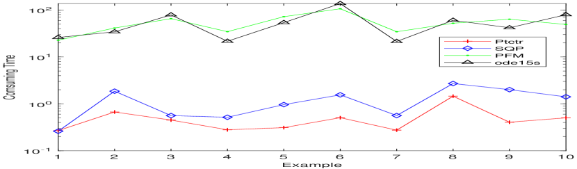
Figure 1: The consumed CPU time (s) of Ptctr,   SQP,   PFM,   ode15s for test problems with $n\approx 1000$.

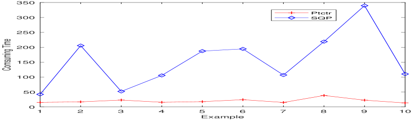
Figure 2: The consumed CPU time (s) of Ptctr,   SQP for test problems with $n\approx 5000$.

4.2 The Visual-Inertial Navigation Localization Problems

In this subsection, in order to verify the performance of Ptctr further, we apply it to a real-world problem which arises from the visual-inertial navigation localization problem when the unmanned aerial vehicle maintains the horizontal flight, and compare it with SQP and ode15s.

When an unmanned aerial vehicle flies with a speed of about 200 m/s at a kilometer altitude for an hour, the positioning error of the pure inertial navigation system is about ten kilometers, which cannot meet the requirement of the positioning accuracy, i.e. less than one kilometer. Therefore, we consider the visual-inertial navigation localization method for this problem EBM2018 ; LLS2020 .

For the visual part, we convert the world coordinate system of landmarks to the camera coordinate system by the pinhole camera model HZ2003 . The pinhole model is illustrated in Figure 3. There are two coordinate systems, which are depicted specifically there. $O$ represents the optical centre of the camera lens and $f_{c}$ refers to the focal length of the camera. The $X^{{}^{\prime}}$-axis and $Y{{}^{\prime}}$ in the camera coordinate system are parallel to the $X$-axis and the $Y$-axis in the world coordinate system, respectively. The position of the $k$-th camera in the world coordinate system is denoted as $(x_{k},\;y_{k},\,z_{k})$. $(x_{ln},\;y_{ln},\;z_{ln})$ denotes the position of the $n$-th landmark in the world coordinate system. The vertical distance between the $n$-th landmark and the camera position of the $k$-th frame is denoted as $h_{n}^{k}=z_{k}-z_{ln}$. $\Delta{x_{n}^{k}},\,\Delta{y_{n}^{k}}$ respectively represent the $X$-axis and $Y$-axis coordinate differences between the $n$-th landmark and the $k$-th camera in the world coordinate system. $(x_{pn}^{k},\;y_{pn}^{k})$ represents the coordinate in the camera coordinate system of the $k$-th frame, which is projected from the $n$-th landmark in the world coordinate system. $\theta$ denotes the line-of-sight angle of the landmark relative to the optical center of the camera.

Figure 3: The pinhole camera model.

Thus, by combining the visual information provided by the camera and the distance information $dist_{hor}$ obtained from Inertial Measurement Units (IMU) between the $k$-th frame camera and the $(k+1)$-th frame camera, we obtain the position of $(x_{k+1},\;y_{k+1})$ of the $(k+1)$-th frame camera in the world coordinate system via solving the following $(k+1)$-th optimization problem:

$$\min_{(x_{k+1},\;y_{k+1})}\quad \left(\sqrt{(x_{k+1}-x_{k})^{2}+(y_{k+1}-y_{k})^{2}}-dist_{hor}\right)^{2}$$ (82)

subject to $$x_{ln}+\frac{x_{pn}^{k}}{f_{c}}h_{n}^{k}=x_{k},$$

$$y_{ln}+\frac{y_{pn}^{k}}{f_{c}}h_{n}^{k}=y_{k},$$ (83)

$$x_{k+1}-x_{ln}-\frac{x_{pn}^{k+1}}{f_{c}}h_{n}^{k}=\frac{\Delta{h_{k}^{k+1}}}{f_{c}}x_{pn}^{k+1},$$

$$y_{k+1}-y_{ln}-\frac{y_{pn}^{k+1}}{f_{c}}h_{n}^{k}=\frac{\Delta{h_{k}^{k+1}}}{f_{c}}y_{pn}^{k+1},$$

where $(x_{k+1},\,y_{k+1})$, $(x_{k},\,y_{k})$ respectively represent the $x$-$y$ axis coordinates of the camera at the $(k+1)$-th frame and the $k$-th frame in the world coordinate system, $(x_{ln},\,y_{ln})$ represents the coordinate of the $n$-th landmark in the world coordinate system, and $(x_{pn}^{k},\,y_{pn}^{k})$, $(x_{pn}^{k+1},\,y_{pn}^{k+1})$ respectively represent the coordinates in the camera coordinate system at the $k$-th frame and the $(k+1)$-th frame, which are projected from the $n$-th landmark in the world coordinate system. In equation (83), $\Delta{h_{k}^{k+1}}$ is the altitude difference obtained by an altimeter between the $k$-th camera position and the $(k+1)$-th camera position, and $dist_{hor}$ represents the horizontal Euclidean distance provided by the IMU between the $k$-th camera position and the $(k+1)$-th camera position.

For the optimization problem (82)-(83), $(x_{k+1},\;y_{k+1})$, $(x_{ln},\;y_{ln})$ and $\Delta{h_{k}^{k+1}}$ are unknown. Obviously, this is an under-determined system if we only use one landmark and we can not uniquely determine the position $(x_{k+1},\;y_{k+1})$ of the camera at the $(k+1)$-th frame. Therefore, we use five landmarks to determine the position of the camera at the $(k+1)$-th frame, and rearrange the constraint system (83) as follows:

$$A_{k+1}w=b_{k+1},\;A_{k+1}=\begin{bmatrix}B&C_{1}&O&O&O&O\\ B&O&C_{2}&O&O&O\\ B&O&O&C_{3}&O&O\\ B&O&O&O&C_{4}&O\\ B&O&O&O&O&C_{5}\\ \end{bmatrix},$$ (84)

where $O\in\Re^{4\times 3}$ represents a zero matrix, and matrix $B$, matrices $C_{n}\,(n=1,\,2,\,\ldots,\,5)$, the constant vector $b_{k+1}$, and the variable $w$ are defined as follows:

$$\hskip 56.9055ptB=\begin{bmatrix}0&0\\ 0&0\\ 1&0\\ 0&1\\ \end{bmatrix},\;C_{n}=\begin{bmatrix}1&0&\frac{x_{pn}^{k}}{f_{c}}\\ 0&1&\frac{y_{pn}^{k}}{f_{c}}\\ -1&0&-\frac{x_{pn}^{k+1}}{f_{c}}\\ 0&-1&-\frac{y_{pn}^{k+1}}{f_{c}}\\ \end{bmatrix},\;n=1,\,2,\,\ldots,\,5,$$

$$b_{k+1}=\left[x_{k},\,y_{k},\,\frac{\Delta{h_{k}^{k+1}}}{f_{c}}x_{p1}^{k+1},\,\frac{\Delta{h_{k}^{k+1}}}{f_{c}}y_{p1}^{k+1},\,\ldots,\,x_{k},\,y_{k},\,\frac{\Delta{h_{k}^{k+1}}}{f_{c}}x_{p5}^{k+1},\,\frac{\Delta{h_{k}^{k+1}}}{f_{c}}y_{p5}^{k+1}\right]^{T},$$

$$w=[x_{k+1},\,y_{k+1},\,x_{l1},\,y_{l1},\,h_{1}^{k},\,\ldots,\,x_{l5},\,y_{l5},\,h_{5}^{k}]^{T}.$$

After simple calculations, we know that the rank of the linear system (84) is deficient when $\Delta h_{k}^{k+1}=0$, where $\Delta h_{k}^{k+1}$ represents the altitude difference between the $k$-th frame and the $(k+1)$-th frame of the camera.

Due to the measurement error for a real-world problem, the linear system (84) has the following general form:

$$A_{k+1}(\varepsilon)w=b_{k+1}(\varepsilon),$$ (85)

where $A_{k+1}(\varepsilon)$ includes the visual measurement error $\varepsilon_{\theta}$ and the altimeter measurement error $\varepsilon_{h}$, $b_{k+1}(\varepsilon)$ is the constant vector with noisy data. Thus, the visual-inertial navigation localization problem (82)-(84) is extended by the following linearly equality-constrained optimization problem with noisy data:

$$\min_{w\in\Re^{17}}\quad f_{k}(w)=\left(\sqrt{(x_{k+1}-x_{k})^{2}+(y_{k+1}-y_{k})^{2}}-dist_{hor,\varepsilon}\right)^{2}$$ (86)

subject to $$A_{k+1}(\varepsilon)s=b_{k+1}(\varepsilon),$$ (87)

where matrix $A_{k+1}(\varepsilon)$ and vector $b_{k+1}(\varepsilon)$ are defined by equation (84).

After establishing the mathematical model (86)-(87) of the visual-inertial navigation localization problem, we simulate the trajectories of the unmanned aerial vehicle maintaining the horizontal flight. By using the optimization method to solve the linearly equality-constrained optimization problem (86)-(87) at every sampling time, we obtain the error propagation of the unmanned aerial vehicle flying for one hour.

According to the given condition from the industry, we assume that the unmanned aerial vehicle flies horizontally for an hour at an altitude of 1200 meters with speed 235 meters per second and the sampling period is half a second. The camera focal length $f_{c}$ is set by $f_{c}=24\times 10^{-3}$ meter. We simulate three simple trajectories with or without measurement errors. The first trajectory is represented as follows:

$$\text{trj 1:}\;(x_{k},\,y_{k},\,z_{k})=(0,\,117.5\,k,\,1200),\;k=1,\,2,\,\ldots,7200.$$ (88)

The second trajectory is represented as follows:

$$\text{trj 2:}\;(x_{k},\,y_{k},\,z_{k})=\left(\frac{1}{2}d_{k},\,\frac{\sqrt{3}}{2}d_{k},\,1200\right),\;d_{k}=117.5\,k,\;k=1,\,2,\,\ldots,\,1800,$$

$$\text{and}\;(x_{k},\,y_{k},\,z_{k})=\left(\frac{1}{2}d_{1800},\,\frac{\sqrt{3}}{2}d_{1800}+d_{k},\,1200\right),\;d_{k}=117.5\,k,$$

$$k=1801,\,1802,\,\ldots,\,7200.$$ (89)

The third trajectory is represented as follows:

$$\text{trj 3:}\;(x_{k},\,y_{k},\,z_{k})=\left(\frac{1}{2}d_{k},\,\frac{\sqrt{3}}{2}d_{k},\,1200\right),\;d_{k}=117.5\,k,\;k=1,\,2,\,\ldots,\,7200.$$ (90)

Thus, based on the known trajectory, we set the coordinate $(x_{ln},\,y_{ln},\,z_{ln})_{k}$ of the $n$-th landmark observed by the $k$-th camera in the world coordinate system as follows:

$$(x_{ln},\,y_{ln},\,z_{ln})_{k}=\left(x_{k}+\frac{58.75n}{N},\,y_{k}+\frac{58.75n}{N},\,\frac{40n}{N}\right),\;n=1,\,2,\,\ldots,\,N.$$ (91)

According to the principle of pinhole imaging, from equations (83) and (91), we generate the image coordinate $\left(x_{pn}^{k},\,y_{pn}^{k}\right)$ of the $n$-th landmark in the $k$-th camera coordinate system as follows:

$$x_{pn}^{k}=\frac{x_{k}-x_{ln}}{h_{n}^{k}}f_{c},\;y_{pn}^{k}=\frac{y_{k}-y_{ln}}{h_{n}^{k}}f_{c},\;n=1,\,2,\ldots,\,N,$$ (92)

where the altitude difference $h_{n}^{k}$ between the $k$-th camera and the $n$-th landmark in the world coordinate system is computed by $h_{n}^{k}=z_{k}-z_{ln}$. The altitude difference $\Delta{h_{k}^{k+1}}$ between the $k$-th camera position and the $(k+1)$-th camera position is computed by $\Delta{h_{k}^{k+1}}=z_{k+1}-z_{k}$.

First, we simulate three trajectories defined by equations (88)-(90) without measurement errors via using Ptctr, SQP and ode15s respectively to solve a series of optimization problems (86)-(87). The initial point of the $(k+1)$-th optimization problem is set by the optimal solution of the $k$-th optimization problem. The simulation results are presented in Table 3 and Figure 5. From Table 3 and Figure 5, we find the consumed time of Ptctr is about one-fifth of that ot SQP and ode15s, and the trajectories computed by Ptctr and ode15s are more accurate than those computed by SQP.

Generally, the measurement data contain errors. According to the provided industrial parameters, we assume that the measurement error $\varepsilon_{h}$ of altitude satisfies the Gaussian distribution $N(\mu_{h},\;\sigma_{h})$ with the variance $\sigma^{2}_{h}=1$ and the mean $\mu_{h}=0$. We assume that the measurement error $\varepsilon_{d}$ of inertial distance satisfies an uniform distribution on the interval $[-2.57,\;2.57]$, i.e. $dist_{hor,\varepsilon}=dist_{hor}+\varepsilon_{d}$.

The angular error $\varepsilon_{\theta}$ of imaging affects the image coordinate $\left(x_{pn}^{k}(\varepsilon_{\theta}),\;y_{pn}^{k}(\varepsilon_{\theta})\right)$ of the $n$-th landmark $(x_{ln},\,y_{ln},\,z_{ln})_{k}$ in the $k$-th camera coordinate system as follows:

$$\theta_{xn}^{k}=\arctan\left(\frac{x_{k}-x_{ln}}{h_{n}^{k}}\right),\;\theta_{yn}^{k}=\arctan\left(\frac{y_{k}-y_{ln}}{h_{n}^{k}}\right),$$

$$\theta_{xn}^{k}(\varepsilon_{\theta})=\theta_{xn}^{k}+\varepsilon_{\theta},\;\theta_{yn}^{k}(\varepsilon_{\theta})=\theta_{yn}^{k}+\varepsilon_{\theta},$$

$$x_{pn}^{k}(\varepsilon_{\theta})=f_{c}\tan\left(\theta_{xn}^{k}(\varepsilon_{\theta})\right),\;y_{pn}^{k}(\varepsilon_{\theta})=f_{c}\tan\left(\theta_{yn}^{k}(\varepsilon_{\theta})\right),\;n=1,\,2,\ldots,N,$$ (93)

where the altitude difference $h_{n}^{k}$ between the $k$-th camera and the $n$-th landmark in the world coordinate system is computed by $h_{n}^{k}=z_{k}-z_{ln}$. Here, we assume that the angular error $\varepsilon_{\theta}$ satisfies an uniform distribution on the interval $[-0.2,\;0.2]$.

For conforming to the real environment of the unmanned aerial vehicle maintaining the horizontal flight, we simulate three trajectories defined by equations (88)-(90) with measurement errors via using Ptctr, SQP and ode15s respectively to solve a series of optimization problems (86)-(87). The measurement errors $\varepsilon_{h},\;\varepsilon_{d},\;\varepsilon_{\theta}$ are stated by the previous several paragraphs of this subsection. The numerical results are presented in Table 4 and Figure 5. From Table 4 and Figure 5, we find that these three algorithms all work well for this problem and the consumed time of Ptctr is one fifth of that of SQP and ode15s, respectively.

Table 3: The visual-inertial positioning
problems without random errors.

Trajectories	Ptctr	SQP	ode15s
	CPU Time (s)	CPU Time (s)	CPU Time (s)
trj 1	6.908	36.126	36.134
trj 2	6.891	37.608	37.614
trj 3	6.792	38.814	38.821

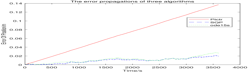
(a) trajectory 1

(b) trajectory 2

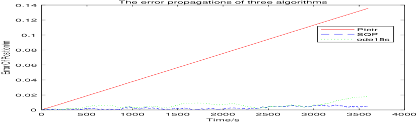
(c) trajectory 3

Figure 4: The visual-inertial positioning
problems without random errors.

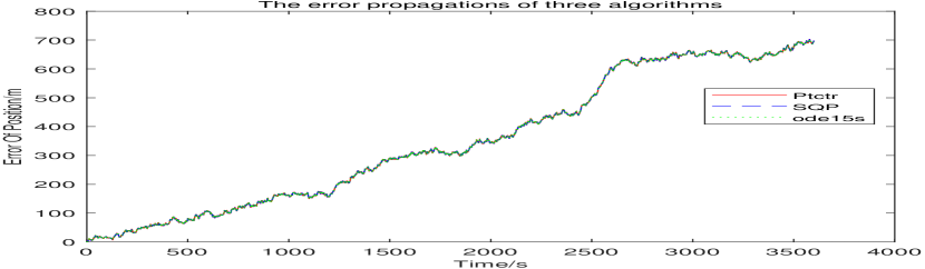
(a) trajectory 1

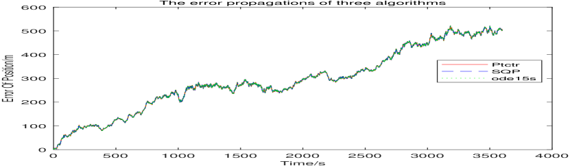
(b) trajectory 2

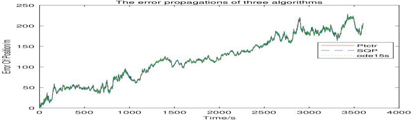
(c) trajectory 3

Figure 5: The visual-inertial positioning problems with random errors.

Table 4: The visual-inertial positioning
problems with random errors.

Trajectories	Ptctr	SQP	ode15s
	CPU Time (s)	CPU Time (s)	CPU Time (s)
trj 1	6.572	37.885	37.893
trj 2	6.695	38.216	38.225
trj 3	5.618	32.023	32.029

5 Conclusion and Future Work

In this paper, we give a continuation method with the trusty time-stepping scheme (Ptctr) for linearly equality-constrained optimization problems. Ptctr only needs to solve a linear system of equations at every iteration, other than the traditional optimization method such as SQP, which needs to solve a quadratic programming subproblem at every iteration. This means that Ptctr can save much more computational time than SQP. Numerical results also show that the consumed time of Ptctr is about one fifth of that of SQP, which is the best method of the three methods (SQP, PFM, ode15s). Furthermore, Ptctr works well for simulating the trajectory of the unmanned aerial vehicle maintaining the horizontal flight for a long time. Therefore, Ptctr is worth investigating further, and we will extend it to the general nonlinear optimization problem in the future.

Appendix A Test Problems

Example 1.

$$\quad m =n/2$$

$$\min_{x\in\Re^{n}}\;f(x) =\sum_{k=1}^{n/2}\;\left(x_{2k-1}^{2}+10x_{2k}^{2}\right),\;\text{subject to}\;x_{2i-1}+x_{2i}=4,\;i=1,\,2,\ldots,\,m.$$

This problem is extended from the problem of Kim2010 . We assume that the feasible initial point is $(2,\,2,\,\ldots,\,2,\,2)$.

Example 2.

$$\quad m =n/3$$

$$\min_{x\in\Re^{n}}\;f(x) =\sum_{k=1}^{n/2}\;\left(\left(x_{2k-1}-2\right)^{2}+2\left(x_{2k}-1\right)^{4}\right)-5,\;\text{subject to}\;x_{3i-2}+4x_{3i-1}+2x_{3i}=3,\;i=1,\,2,\ldots,\,n/3.$$

We assume that the infeasible initial point is $(-0.5,\,1.5,\,1,\,0,\,\ldots,\,0,\,0)$.

Example 3.

$$\quad m =(2/3)n$$

$$\min_{x\in\Re^{n}}\;f(x) =\sum_{k=1}^{n}\;x_{k}^{2},\;\text{subject to}\;x_{3i-2}+2x_{3i-1}+x_{3i}=1,\;2x_{3i-2}-x_{3i-1}-3x_{3i}=4,\;i=1,\,2,\ldots,\,n/3.$$

This problem is extended from the problem of Osborne2016 . The infeasible initial point is $(1,\,0.5,\,-1,\,\ldots,\,1,\,0.5,\,-1)$.

Example 4.

$$\quad m =n/2$$

$$\min_{x\in\Re^{n}}\;f(x) =\sum_{k=1}^{n/2}\;\left(x_{2k-1}^{2}+x_{2k}^{6}\right)-1,\;\text{subject to}\;x_{2i-1}+x_{2i}=1,\;i=1,\,2,\,\ldots,\,n/2.$$

This problem is modified from the problem of MAK2019 . We assume that the infeasible initial point is $(1,\,1,\,\ldots,\,1)$.

Example 5.

$$\quad m =n/2$$

$$\min_{x\in\Re^{n}}\;f(x) =\sum_{k=1}^{n/2}\;\left(\left(x_{2k-1}-2\right)^{4}+2\left(x_{2k}-1\right)^{6}\right)-5,\;\text{subject to}\;x_{2i-1}+4x_{2i}=3,\;i=1,\,2,\,\ldots,\,m.$$

We assume that the feasible initial point is $(-1,\,1,\,-1,\,1,\,\ldots,\,-1,\,1)$.

Example 6.

$$\quad m =(2/3)n$$

$$\min_{x\in\Re^{n}}\;f(x) =\sum_{k=1}^{n/3}\;\left(x_{3k-2}^{2}+x_{3k-1}^{4}+x_{3k}^{6}\right),$$

subject to $${x_{3i-2}}+2{x_{3i-1}}+{x_{3i}}=1,\;2{x_{3i-2}}-{x_{3i-1}}-3{x_{3i}}=4,\;i=1,\,2,\,\ldots,\,m/2.$$

This problem is extended from the problem of Osborne2016 . We assume that the infeasible initial point is $(2,\,0,\,\ldots,\,0)$.

Example 7.

$$\quad m =n/2$$

$$\min_{x\in\Re^{n}}\;f(x) =\sum_{k=1}^{n/2}\;\left(x_{2k-1}^{4}+3x_{2k}^{2}\right),\;\text{subject to}\;x_{2i-1}+x_{2i}=4,\;i=1,\,2,\,\ldots,\,n/2.$$

This problem is extended from the problem of Carlberg2009 . We assume that the infeasible initial point is $(2,\,2,\,0,\,\ldots,\,0,\,0)$.

Example 8.

$$\quad m =n/3$$

$$\min_{x\in\Re{{}^{n}}}\;f(x) =\sum_{k=1}^{n/3}\;\left(x_{3k-2}^{2}+x_{3k-2}^{2}\,x_{3k}^{2}+2x_{3k-2}\,x_{3k-1}+x_{3k-1}^{4}+8x_{3k-1}\right),$$

subject to $$2x_{3i-2}+5x_{3i-1}+x_{3i}=3,\;i=1,\,2,\,\ldots,\,m.$$

We assume that the infeasible initial point is $(1.5,\,0,\,0,\,\ldots,\,0)$.

Example 9.

$$\quad m =n/2$$

$$\min_{x\in\Re^{n}}\;f(x) =\sum_{k=1}^{n/2}\;\left(x_{2k-1}^{4}+10x_{2k}^{6}\right),\;\text{subject to}\;x_{2i-1}+x_{2i}=4,\;i=1,\,2,\,\ldots,\,m.$$

This problem is extended from the problem of Kim2010 . We assume that the feasible initial point is $(2,\,2,\,\ldots,\,2,\,2)$.

Example 10.

$$\quad m =n/3$$

$$\min_{x\in\Re^{n}}\;f(x) =\sum_{k=1}^{n/3}\;\left(x_{3k-2}^{8}+x_{3k-1}^{6}+x_{3k}^{2}\,\right),\;\text{subject to}\;x_{3i-2}+2x_{3i-1}+2x_{3i}=1,\;i=1,\,2,\,\ldots,\,m.$$

This problem is modified from the problem of Yamashita1980 . The feasible initial point is $(1,\,0,\,0,\,\ldots,\,1,\,0,\,0)$.