Deep Completion Autoencoders for
Radio Map Estimation

Abstract

Radio maps provide metrics such as power spectral density for every location in a geographic area and find numerous applications such as UAV communications, interference control, spectrum management, resource allocation, and network planning to name a few. Radio maps are constructed from measurements collected by spectrum sensors distributed across space. Since radio maps are complicated functions of the spatial coordinates due to the nature of electromagnetic wave propagation, model-free approaches are strongly motivated. Nevertheless, all existing schemes for radio occupancy map estimation rely on interpolation algorithms unable to learn from experience. In contrast, this paper proposes a novel approach in which the spatial structure of propagation phenomena such as shadowing is learned beforehand from a data set with measurements in other environments. Relative to existing schemes, a significantly smaller number of measurements is therefore required to estimate a map with a prescribed accuracy. As an additional novelty, this is also the first work to estimate radio occupancy maps using deep neural networks. Specifically, a fully convolutional deep completion autoencoder architecture is developed to effectively exploit the manifold structure of this class of maps.

I Introduction

Spectrum cartography comprises a collection of techniques to construct radio maps, which provide channel metrics such as received signal power, interference power, power spectral density (PSD), electromagnetic absorption, or channel gain across a geographic area; see e.g. [2, 3, 4, 5]. Besides applications related to localization [3, 6] and radio tomography [7, 8], radio maps find a myriad of applications in wireless communications such as network planning, interference coordination, power control, spectrum management, resource allocation, handoff procedure design, dynamic spectrum access, and cognitive radio; see e.g. [9, 10, 11]. More recently, radio maps have been widely recognized as an enabling technology for UAV communications because they allow autonomous UAVs to account for communication constraints when planning a mission; see e.g. [12, 13, 14, 15].

The problem of predicting the received signal strength at a given location or channel gain between a pair of locations, termed radio propagation prediction, has been initially tackled through modeling. This includes empirical models [16, Ch. 2], the dominant path model[17], and the more sophisticated ray-tracing algorithms (see e.g. [18]) to name a few. Due to the inherent limitations of modeling, data-driven alternatives that learn from channel measurements have been recently developed [19, 20, 21, 22, 23, 24, 25]. The main limitation of these approaches is that the number, locations, and (generally) power of all transmitters need to be known. Besides, these data-driven approaches are sensitive to interference since they assume that the measurements contain only power received from a single transmitter with known power and location. Furthermore, most of these schemes for radio propagation prediction suffer from a large computational complexity when predictions must be provided at a large set of locations.

To address these limitations, approaches for radio (occupancy) map estimation target the aggregate power from all active transmitters and predict power or channel gain across the area of interest without knowledge of the number, locations, and power of the transmitters. This is a critical benefit especially in scenarios with a large number of transmitters, as in the uplink of a cellular network or in device-to-device communications, since this information is typically unreliable and costly to maintain. Most approaches for radio occupancy map estimation build upon some interpolation algorithm. For example, power maps have been constructed through kriging [2, 27, 26, 28], compressive sensing [4], dictionary learning [29, 30], matrix completion [31], Bayesian models [32], radial basis functions [33, 34], and kernel methods [35]. PSD map estimators have been developed using sparse learning [3], thin-plate spline regression [36], kernel-based learning [37, 11], and tensor completion [38, 39]. Related approaches have been adopted in [40, 41, 8, 42] to propose channel-gain map estimators. Unfortunately, none of these approaches for radio occupancy map estimation can learn from experience, which suggests that their estimation performance can be significantly improved along this direction.

To this end, this work puts forth a data-driven paradigm for radio occupancy map estimation. The idea is to learn the spatial structure of relevant propagation phenomena such as shadowing, reflection, and diffraction using a data set of past measurements in different environments. Intuitively, learning how these phenomena evolve across space can significantly reduce the number of measurements required to achieve a given estimation accuracy. This is a critical aspect since the time interval in which measurements are collected needs to be sufficiently short relative to the temporal variations of the target map in real-world scenarios (coherence time). The main contribution of this work is to build upon this idea to develop a PSD map estimation algorithm based on a deep neural network. To cope with the variable number of measurements, a tensor completion task is formulated based on a spatial discretization of the area of interest and addressed by means of a completion network with an encoder-decoder architecture, which belongs to a broad family of networks with well-documented merits in other wireless communications contexts [44]. This structure is motivated by the observation that radio maps lie close to a low-dimensional manifold embedded in a high-dimensional space. Extensive experiments using a realistic data set obtained with Remcom’s Wireless InSite simulator reveal that the proposed algorithm markedly outperforms state-of-the-art radio map estimators and exhibits strong out-of-sample generalization capabilities. This data set is available along with the code at https://github.com/yvestegnya2/deep-
autoencoders-cartography.

The novelty of this work is twofold: (i) it is the first to propose data-driven radio occupancy map estimation by learning from experience; (ii) it is the first to propose a deep learning algorithm for radio occupancy map estimation.

The rest of this paper is organized as follows. Sec. II formulates the problem of PSD map estimation. Sec. III introduces the aforementioned data-driven radio map estimation paradigm and proposes a deep neural network architecture based on completion autoencoders. Simulations, conclusions, and a discussion are provided in Secs. IV and V.

Notation: $|\mathcal{A}|$ denotes the cardinality of set $\mathcal{A}$. Bold uppercase (lowercase) letters denote matrices or tensors (column vectors), $[\bm{a}]_{i}$ is the $i$-th entry of vector $\bm{a}$, $[\bm{A}]_{i,j}$ is the $(i,j)$-th entry of matrix $\bm{A}$, and $[\bm{B}]_{i,j,k}$ is the $(i,j,k)$-th entry of tensor $\bm{B}$. Finally, $\bm{A}^{\top}$ is the transpose of matrix $\bm{A}$.

II PSD Map Estimation Problem

This section formulates the problem of PSD map estimation. The problem where power maps are estimated can be recovered as a special case of PSD map estimation in a single frequency.

Consider ${{\color[rgb]{0,0,0}S}}$ transmitters, or sources, located in a geographic region of interest $\mathcal{X}\subset\mathbb{R}^{2}$ and operating in a certain frequency band. Let ${{\color[rgb]{0,0,0}\Upsilon}}_{{{\color[rgb]{0,0,0}s}}}(f)$ denote the transmit PSD of the ${{\color[rgb]{0,0,0}s}}$-th source and let $H_{{{\color[rgb]{0,0,0}s}}}(\bm{x},f)$ represent the frequency response of the channel between the ${{\color[rgb]{0,0,0}s}}$-th source and a receiver with an isotropic antenna at location $\bm{x}\in\mathcal{X}$. Both ${{\color[rgb]{0,0,0}\Upsilon}}_{{{\color[rgb]{0,0,0}s}}}(f)$ and $H_{{{\color[rgb]{0,0,0}s}}}(\bm{x},f)$ are assumed to remain constant over time; see Remark 2.

If the ${{\color[rgb]{0,0,0}S}}$ signals are uncorrelated, the PSD at $\bm{x}\in\mathcal{X}$ is

$${\color[rgb]{0,0,0}\Psi}(\bm{x},f)=\textstyle\sum_{{{\color[rgb]{0,0,0}s}}=1}^{{{\color[rgb]{0,0,0}S}}}{{\color[rgb]{0,0,0}\Upsilon}}_{{{\color[rgb]{0,0,0}s}}}(f)|H_{{{\color[rgb]{0,0,0}s}}}(\bm{x},f)|^{2}+\upsilon(\bm{x},f),$$ (1)

where $\upsilon(\bm{x},f)$ models thermal noise, background radiation noise, and interference from remote sources. A certain number of devices with sensing capabilities, e.g. user terminals in a cellular network, collect PSD measurements $\{{{\color[rgb]{0,0,0}\tilde{\color[rgb]{0,0,0}\Psi}}}(\bm{x}_{n},f)\}_{n=1}^{N}$ at $N$ locations $\{\bm{x}_{n}\}_{n=1}^{N}\subset\mathcal{X}$ and at a finite set of frequencies $f\in\mathcal{F}$; see also Remark 2. These frequency measurements can be obtained using e.g. periodograms or spectral analysis methods such as the Bartlett or Welch method [45].

These measurements are sent to a fusion center, which may be e.g. a base station, a mobile user, or a cloud server, depending on the application. Given $\{(\bm{x}_{n},{{\color[rgb]{0,0,0}\tilde{\color[rgb]{0,0,0}\Psi}}}(\bm{x}_{n},f)),~{}n=1,\ldots,N,~{}f\in\mathcal{F}\}$, the problem that the fusion center needs to solve is to find an estimate ${{\color[rgb]{0,0,0}\hat{\color[rgb]{0,0,0}\Psi}}}(\bm{x},f)$ of ${\color[rgb]{0,0,0}\Psi}(\bm{x},f)$ at every location $\bm{x}\in\mathcal{X}$ and frequency $f\in\mathcal{F}$. Function ${\color[rgb]{0,0,0}\Psi}(\bm{x},f)$ is typically referred to as the true map, whereas ${{\color[rgb]{0,0,0}\hat{\color[rgb]{0,0,0}\Psi}}}(\bm{x},f)$ is the map estimate. An algorithm that produces ${{\color[rgb]{0,0,0}\hat{\color[rgb]{0,0,0}\Psi}}}(\bm{x},f)$ is termed map estimator.

A natural error metric is the energy $\sum_{f}\int_{\mathcal{X}}|{\color[rgb]{0,0,0}\Psi}(\bm{x},f)-{{\color[rgb]{0,0,0}\hat{\color[rgb]{0,0,0}\Psi}}}(\bm{x},f)|^{2}d\bm{x}$. One can quantify the performance of a map estimator in terms of the expectation of this error for a given $N$ or, equivalently, in terms of the minimum $N$ required to guarantee that the expected error is below a prescribed bound.

Remark 1

The channel $H_{{{\color[rgb]{0,0,0}s}}}(\bm{x},f)$ is usually decomposed into path loss, shadowing, and fast fading components. Whereas path loss and shadowing typically vary in a scale of meters, fast fading changes in a scale comparable to the wavelength. Since contemporary wireless communication systems utilize wavelengths in the order of millimeters or centimeters, estimating this fast fading component would require knowing the sensor locations $\{\bm{x}_{n}\}_{n}$ with an accuracy in the order of millimeters, which is not possible e.g. with current global navigation satellite systems (GNSSs). Thus, it is customary to assume that the effects of fast fading have been averaged out and, hence, $H_{{{\color[rgb]{0,0,0}s}}}(\bm{x},f)$ captures only path loss and shadowing. This is especially well-motivated in scenarios where sensors acquire measurements while moving.

Remark 2

${{\color[rgb]{0,0,0}\Upsilon}}_{{{\color[rgb]{0,0,0}s}}}(f)$ and $H_{{{\color[rgb]{0,0,0}s}}}(\bm{x},f)$ can be assumed constant over time so long as the measurements are collected within an interval of shorter length than the channel coherence time and time scale of changes in ${{\color[rgb]{0,0,0}\Upsilon}}_{{{\color[rgb]{0,0,0}s}}}(f)$. The latter is highly dependent on the specific application. For example, one expects that significant variations in DVB-T bands occur in a scale of several months, whereas ${{\color[rgb]{0,0,0}\Upsilon}}_{{{\color[rgb]{0,0,0}s}}}(f)$ in LTE bands may change in a scale of milliseconds. In any case, a sensor that moves may collect multiple measurements over this interval where ${{\color[rgb]{0,0,0}\Upsilon}}_{{{\color[rgb]{0,0,0}s}}}(f)$ and $H_{{{\color[rgb]{0,0,0}s}}}(\bm{x},f)$ remain approximately constant, which could render the number of measurements significantly larger than the number of sensors.

III Data-Driven Radio Map Estimation

All existing occupancy map estimators rely on interpolation algorithms that do not learn from experience. However, it seems natural that an algorithm can be trained to learn how to solve the problem in Sec. II using a record of past measurements, possibly in other geographic regions. Specifically, besides ${{\color[rgb]{0,0,0}\mathcal{D}}}{:=}\{(\bm{x}_{n},{{\color[rgb]{0,0,0}\tilde{\color[rgb]{0,0,0}\Psi}}}(\bm{x}_{n},f)),\bm{x}_{n}\in\mathcal{X},~{}f\in\mathcal{F},~{}n=1,\ldots,N\}$, a number of measurement records of the form ${{\color[rgb]{0,0,0}\mathcal{D}}}_{t}{:=}\{(\bm{x}_{nt},{{\color[rgb]{0,0,0}\tilde{\color[rgb]{0,0,0}\Psi}}}_{t}(\bm{x}_{nt},f)),~{}\bm{x}_{nt}\in\mathcal{X}_{t},~{}f\in\mathcal{F},~{}n=1,\ldots,N_{t}\}$, $t=1,\ldots,T$, may be available, where ${{\color[rgb]{0,0,0}\mathcal{D}}}_{t}$ contains $N_{t}$ measurements collected in the geographic area $\mathcal{X}_{t}$; see Sec. III-E. With this additional data, a better performance is expected when estimating ${\color[rgb]{0,0,0}\Psi}(\bm{x},f)$.

The rest of this section develops deep learning estimators that address this data-aided formulation. To this end, Sec. III-A starts by reformulating the problem at hand as a tensor completion task amenable to application of deep neural networks. Subsequently, Sec. III-B addresses unique aspects of tensor/matrix completion via deep learning. Sec. III-C discusses how to exploit structure in the frequency domain. Finally, Secs. III-D and III-E respectively describe how to learn the spatial structure of propagation phenomena via the notion of completion autoencoders and how these networks can be trained in real-world scenarios.

III-A Map Estimation as a Tensor Completion Task

Observe that $N$ and $N_{t}$ depend on the number and movement of the sensors relative to the time-scale of temporal variations in ${\color[rgb]{0,0,0}\Psi}(\bm{x},f)$ and ${\color[rgb]{0,0,0}\Psi}_{t}(\bm{x},f)$, respectively; cf. Remark 2. In principle, one could think of using a separate map estimator for each possible value of $N$. Each estimator could be relatively simple since it would always take the same number of inputs. However, such an approach would be highly inefficient in terms of memory, computation, and prone to erratic behavior since each estimator would have different parameters or be trained with a different data set. Thus, it is more practical to rely on a single estimator that can accommodate an arbitrary number of measurements.

Given their well-documented merits in a number of tasks, deep neural networks constitute a sensible framework to develop radio map estimators. However, regular feedforward neural networks cannot directly accommodate inputs of variable size. To bypass this difficulty, the approach pursued here relies on a spatial discretization amenable to application of feedforward architectures [46, Ch. 6]. Similar discretizations have been applied in [8, 47, 31, 38].

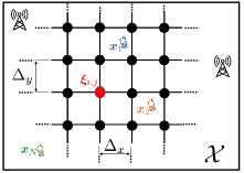
Figure 1: Model setup and area discretization.

To introduce the appropriate notation, this discretization is briefly outlined for ${{\color[rgb]{0,0,0}\mathcal{D}}}$; the extension to ${{\color[rgb]{0,0,0}\mathcal{D}}}_{t}$ follows the same lines. Define an $N_{y}\times N_{x}$ rectangular grid over $\mathcal{X}$, as depicted in Fig. 1. This grid comprises points ${{\color[rgb]{0,0,0}\bm{\xi}}}_{i,j}$ evenly spaced by $\Delta_{x}$ and $\Delta_{y}$ along the $x$- and $y$-axes respectively, that is, the $(i,j)$-th grid point is given by ${{\color[rgb]{0,0,0}\bm{\xi}}}_{i,j}:=\left[j\Delta_{x},~{}i\Delta_{y}\right]^{\top}$, with $~{}i=1,\ldots,N_{y},~{}j=1,\ldots,N_{x}$. For future usage, define $\mathcal{A}_{i,j}\subset\{1,\ldots,N\}$ as the set containing the indices of the measurement locations assigned to the $(i,j)$-th grid point by the criterion of minimum distance, i.e., $n\in\mathcal{A}_{i,j}$ iff $||{{\color[rgb]{0,0,0}\bm{\xi}}}_{i,j}-\bm{x}_{n}||\leq||{{\color[rgb]{0,0,0}\bm{\xi}}}_{i^{\prime},j^{\prime}}-\bm{x}_{n}||~{}\forall i^{\prime},j^{\prime}$.

This grid induces a discretization of ${\color[rgb]{0,0,0}\Psi}(\bm{x},f)$ along the $\bm{x}$ variable. One can therefore collect the true PSD values at the grid points in matrix $\bm{{\color[rgb]{0,0,0}\Psi}}(f)\in\mathbb{R}^{N_{y}\times N_{x}}$, $f\in\mathcal{F}$, whose $(i,j)$-th entry is given by $\left[\bm{{\color[rgb]{0,0,0}\Psi}}(f)\right]_{i,j}={\color[rgb]{0,0,0}\Psi}({{\color[rgb]{0,0,0}\bm{\xi}}}_{i,j},f)$. By letting $\mathcal{F}=\{f_{1},\ldots,f_{N_{f}}\}$, it is also possible to concatenate these matrices to form the tensor $\bm{{\color[rgb]{0,0,0}\Psi}}\in\mathbb{R}^{N_{y}\times N_{x}\times N_{f}}$, where $\left[\bm{{\color[rgb]{0,0,0}\Psi}}\right]_{i,j,n_{f}}={\color[rgb]{0,0,0}\Psi}({{\color[rgb]{0,0,0}\bm{\xi}}}_{i,j},f_{n_{f}})$, $n_{f}=1,\ldots,N_{f}$. For short, the term true map will either refer to ${\color[rgb]{0,0,0}\Psi}(\bm{x},f)$ or $\bm{{\color[rgb]{0,0,0}\Psi}}$.

Similarly, one can collect the measurements in a tensor of the same dimensions. Informally, if the grid is sufficiently fine ($\Delta_{x}$ and $\Delta_{y}$ are sufficiently small), it holds that $\bm{x}_{n}\approx{{\color[rgb]{0,0,0}\bm{\xi}}}_{i,j}$ $\forall n\in\mathcal{A}_{i,j}$ and, correspondingly, ${\color[rgb]{0,0,0}\Psi}(\bm{x}_{n},f)\approx{\color[rgb]{0,0,0}\Psi}({{\color[rgb]{0,0,0}\bm{\xi}}}_{i,j},f)$ $\forall n\in\mathcal{A}_{i,j}$. It follows that, ${\color[rgb]{0,0,0}\Psi}({{\color[rgb]{0,0,0}\bm{\xi}}}_{i,j},f)\approx({1}/{|\mathcal{A}_{i,j}|)}\sum_{n\in\mathcal{A}_{i,j}}{\color[rgb]{0,0,0}\Psi}(\bm{x}_{n},f)$ whenever $|\mathcal{A}_{i,j}|>0$. Therefore, it makes sense to aggregate the measurements assigned to ${{\color[rgb]{0,0,0}\bm{\xi}}}_{i,j}$ as ${{\color[rgb]{0,0,0}\tilde{\color[rgb]{0,0,0}\Psi}}}({{\color[rgb]{0,0,0}\bm{\xi}}}_{i,j},f){:=}({1}/{|\mathcal{A}_{i,j}|})\sum_{n\in\mathcal{A}_{i,j}}{{\color[rgb]{0,0,0}\tilde{\color[rgb]{0,0,0}\Psi}}}(\bm{x}_{n},f)$. Observe that aggregation of this form could alleviate the effects of small scale fading in the channel; see Remark 1. Conversely, when $|\mathcal{A}_{i,j}|=0$, there are no measurements associated with ${{\color[rgb]{0,0,0}\bm{\xi}}}_{i,j}$, in which case one says that there is a miss at ${{\color[rgb]{0,0,0}\bm{\xi}}}_{i,j}$. Upon letting $\Omega\subset\{1,\ldots,N_{y}\}\times\{1,\ldots,N_{x}\}$ be such that $(i,j)\in\Omega$ iff $|\mathcal{A}_{i,j}|>0$, all aggregated measurements ${{\color[rgb]{0,0,0}\tilde{\color[rgb]{0,0,0}\Psi}}}({{\color[rgb]{0,0,0}\bm{\xi}}}_{i,j},f)$ can be collected into ${{\tilde{\bm{{\color[rgb]{0,0,0}\Psi}}}}}(f)\in\mathbb{R}^{N_{y}\times N_{x}}$, defined as $[{{\tilde{\bm{{\color[rgb]{0,0,0}\Psi}}}}}(f)]_{i,j}={{\color[rgb]{0,0,0}\tilde{\color[rgb]{0,0,0}\Psi}}}({{\color[rgb]{0,0,0}\bm{\xi}}}_{i,j},f)$ if $(i,j)\in\Omega$ and $[\tilde{\bm{{\color[rgb]{0,0,0}\Psi}}}(f)]_{i,j}=0$ otherwise. Note that misses have been filled with zeroes, but other values could have been used.

When $(i,j)\in\Omega$, the values of $[\tilde{\bm{{\color[rgb]{0,0,0}\Psi}}}(f)]_{i,j}$ and $[{\bm{{\color[rgb]{0,0,0}\Psi}}}(f)]_{i,j}$ differ due to the error introduced by the spatial discretization as well as due to the measurement error incurred when measuring ${\color[rgb]{0,0,0}\Psi}(\bm{x}_{n},f),~{}n\in\mathcal{A}_{i,j}$. The latter is caused mainly by the finite time devoted by sensors to take measurements, their movement, localization errors, and possible variations of ${\color[rgb]{0,0,0}\Psi}(\bm{x}_{n},f)$ over time.

As before, the matrices ${{\tilde{\bm{{\color[rgb]{0,0,0}\Psi}}}}}(f),~{}f=1,\ldots,N_{f}$ can be concatenated to form ${{\tilde{\bm{{\color[rgb]{0,0,0}\Psi}}}}}\in\mathbb{R}^{N_{y}\times N_{x}\times N_{f}}$, where $[{{\tilde{\bm{{\color[rgb]{0,0,0}\Psi}}}}}]_{i,j,n_{f}}=[{{\tilde{\bm{{\color[rgb]{0,0,0}\Psi}}}}}(f_{n_{f}})]_{i,j}$. For short, this tensor will be referred to as the sampled map. With this notation, the cartography problem stated in Sec. II will be approximated as estimating $\bm{{\color[rgb]{0,0,0}\Psi}}$ given $\Omega$ and ${{\tilde{\bm{{\color[rgb]{0,0,0}\Psi}}}}}$,

III-B Completion Networks for Radio Map Estimation

The data in the problem formulation at the end of Sec. III-A cannot be handled by plain feedforward neural networks since they cannot directly accommodate input misses and set-valued inputs like $\Omega$. This section explores how to bypass this difficulty.

Before that, a swift refresh on deep learning is in order. A feedforward deep neural network is a function ${\color[rgb]{0,0,0}p_{\bm{w}}}$ that can be expressed as the composition ${\color[rgb]{0,0,0}p_{\bm{w}}}({{\color[rgb]{0,0,0}\bm{\Phi}}})={\color[rgb]{0,0,0}p}^{{\color[rgb]{0,0,0}(}{\color[rgb]{0,0,0}L}{\color[rgb]{0,0,0})}}_{\bm{w}_{{\color[rgb]{0,0,0}L}}}({\color[rgb]{0,0,0}p}^{{\color[rgb]{0,0,0}(}{\color[rgb]{0,0,0}L}-1{\color[rgb]{0,0,0})}}_{\bm{w}_{{\color[rgb]{0,0,0}L}-1}}(\ldots{\color[rgb]{0,0,0}p}^{{\color[rgb]{0,0,0}(}1{\color[rgb]{0,0,0})}}_{\bm{w}_{1}}({{\color[rgb]{0,0,0}\bm{\Phi}}})))$ of layer functions ${\color[rgb]{0,0,0}p}^{{\color[rgb]{0,0,0}(}{{\color[rgb]{0,0,0}l}}{\color[rgb]{0,0,0})}}_{\bm{w}_{{\color[rgb]{0,0,0}l}}}$, where ${{\color[rgb]{0,0,0}\bm{\Phi}}}$ is the input. Although there is no commonly agreed definition of layer function, it is typically formed by concatenating simple scalar-valued functions termed neurons that implement a linear aggregation followed by a non-linear function known as activation [46]. The term neuron stems from the resemblance between these functions and certain simple functional models for biological neurons. Similarly, there is no general agreement on which values of ${\color[rgb]{0,0,0}L}$ qualify for ${\color[rgb]{0,0,0}p_{\bm{w}}}$ to be regarded a deep neural network, but in practice ${\color[rgb]{0,0,0}L}$ may range from tens to thousands. With vector $\bm{w}_{{\color[rgb]{0,0,0}l}}$ containing the parameters, or weights, of the ${{\color[rgb]{0,0,0}l}}$-th layer, the parameters of the entire network can be stacked as $\bm{w}{:=}[\bm{w}_{1}^{\top},\ldots,\bm{w}_{{\color[rgb]{0,0,0}L}}^{\top}]^{\top}\in\mathbb{R}^{N_{w}}$. These parameters are learned using a training set in a process termed training.

The rest of this section designs ${\color[rgb]{0,0,0}p}^{{\color[rgb]{0,0,0}(}1{\color[rgb]{0,0,0})}}_{\bm{w}_{1}}$ to cope with missing data, whereas Secs. III-C and III-D will address the design of the other layers. Throughout, the training examples will be represented by $\{({{\tilde{\bm{{\color[rgb]{0,0,0}\Psi}}}}}_{t},\Omega_{t})\}_{t=1}^{T}$, where ${{\tilde{\bm{{\color[rgb]{0,0,0}\Psi}}}}}_{t}$ and $\Omega_{t}$ are obtained from ${{\color[rgb]{0,0,0}\mathcal{D}}}_{t}$ by applying the procedure described in Sec. III-A.

The desired estimator should obtain $\bm{{\color[rgb]{0,0,0}\Psi}}$ as a function of the measurements in ${{\tilde{\bm{{\color[rgb]{0,0,0}\Psi}}}}}$ and $\Omega$. Recall that only a subset of the entries of ${{\tilde{\bm{{\color[rgb]{0,0,0}\Psi}}}}}$ contain actual measurements, whereas the rest have been filled, e.g. with zeros. Unfortunately, it is not directly possible to accommodate variable input supports in regular feedforward neural networks. However, as a first attempt, one could think of directly feeding ${{\tilde{\bm{{\color[rgb]{0,0,0}\Psi}}}}}$ to the neural network and training by only fitting the entries containing measurements as

$$\underset{\bm{w}}{\text{minimize}}\quad \textstyle\frac{1}{T}\sum_{t=1}^{T}\left\|\mathcal{P}_{\Omega_{t}}\left({{\tilde{\bm{{\color[rgb]{0,0,0}\Psi}}}}}_{t}-p_{\bm{w}}({{\tilde{\bm{{\color[rgb]{0,0,0}\Psi}}}}}_{t})\right)\right\|_{F}^{2},$$ (2)

where $||\bm{A}||_{F}^{2}{:=}\sum_{i,j,n_{f}}[\bm{A}]_{i,j,n_{f}}^{2}$ is the squared Frobenius norm of tensor $\bm{A}$ and $\mathcal{P}_{\Omega}(\bm{A})$ is defined by $\left[\mathcal{P}_{\Omega}(\bm{A})\right]_{i,j,n_{f}}=[\bm{A}]_{i,j,n_{f}}$ if $(i,j)\in\Omega$ and $\left[\mathcal{P}_{\Omega}(\bm{A})\right]_{i,j,n_{f}}=0$ otherwise. After (2) is solved, ${{\tilde{\bm{{\color[rgb]{0,0,0}\Psi}}}}}$ could be completed just by evaluating $p_{\bm{w}}({{\tilde{\bm{{\color[rgb]{0,0,0}\Psi}}}}})$. Observe that if the family of candidate functions $\{p_{\bm{w}}:\bm{w}\in\mathbb{R}^{N_{w}}\}$ contains the identity map $p_{\bm{w}}({{\tilde{\bm{{\color[rgb]{0,0,0}\Psi}}}}})={{\tilde{\bm{{\color[rgb]{0,0,0}\Psi}}}}}$, then the minimum of (2) would be attained for such a function. This would clearly render the estimator useless. Thus, one needs to introduce some form of complexity control [49] e.g. by regularization or by limiting the family $\{p_{\bm{w}}:\bm{w}\in\mathbb{R}^{N_{w}}\}$. This work pursues the second strategy by means of an encoder-decoder architecture, as detailed in Sec. III-D.

Because the aforementioned estimator does not account for $\Omega$, poor performance is expected since the network cannot distinguish missing entries from measurements close to the filling value. In the application at hand, one could circumvent this limitation by expressing the entries of ${{\tilde{\bm{{\color[rgb]{0,0,0}\Psi}}}}}$ in natural power units (e.g. Watt) and filling the misses with a negative number such as -1. Unfortunately, the usage of finite-precision arithmetic would introduce large errors in the map estimates and is problematic in our experience. For this reason, expressing ${{\tilde{\bm{{\color[rgb]{0,0,0}\Psi}}}}}$ in logarithmic units such as dBm is preferable. However, in that case, filling misses with negative numbers would not solve the aforementioned difficulty since logarithmic units are not confined to take non-negative values. Hence, a preferable alternative is to complement the input map with a binary mask that indicates which entries are observed, as proposed in the image inpainting literature [50]. Specifically, a mask $\bm{{\color[rgb]{0,0,0}M}}_{\Omega}\in\{0,1\}^{N_{y}\times N_{x}}$ can be used to represent $\Omega$ by setting $[\bm{{\color[rgb]{0,0,0}M}}_{\Omega}]_{i,j}=1$ if $(i,j)\in\Omega$ and $[\bm{{\color[rgb]{0,0,0}M}}_{\Omega}]_{i,j}=0$ otherwise. To simplify notation, let ${{\color[rgb]{0,0,0}{\color[rgb]{0,0,0}\breve{\bm{\Psi}}}}}\in\mathbb{R}^{N_{y}\times N_{x}\times N_{f}+1}$ denote a tensor obtained by concatenating ${{\tilde{\bm{{\color[rgb]{0,0,0}\Psi}}}}}$ and $\bm{{\color[rgb]{0,0,0}M}}_{\Omega}$ along the third dimension. The neural network can therefore be trained as

$$\underset{\bm{w}}{\text{minimize}}\quad \textstyle\frac{1}{T}\sum_{t=1}^{T}\left\|\mathcal{P}_{\Omega_{t}}\left({{\tilde{\bm{{\color[rgb]{0,0,0}\Psi}}}}}_{t}-p_{\bm{w}}({{\color[rgb]{0,0,0}{\color[rgb]{0,0,0}\breve{\bm{\Psi}}}}}_{t})\right)\right\|_{F}^{2},$$ (3)

and, afterwards, a tensor ${{\tilde{\bm{{\color[rgb]{0,0,0}\Psi}}}}}$ can be completed just by evaluating $p_{\bm{w}}({{\color[rgb]{0,0,0}{\color[rgb]{0,0,0}\breve{\bm{\Psi}}}}})$. Then, this scheme is simple to train, inexpensive to test, and exploits information about the location of the misses.

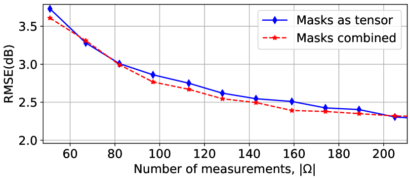
Figure 2: Map estimation RMSE as a function of the number of measurements when the building and measurement masks are separately provided (masks as tensor) or combined into a single mask (masks combined). The training and testing maps were obtained from the Wireless InSite data set; see Sec. IV.

Remark 3

The introduction of a binary mask to indicate the sensor locations suggests an approach along the lines of [20, 23] to accommodate additional side information that may assist in map estimation. For example, one can append an additional mask $\bm{{\color[rgb]{0,0,0}{\color[rgb]{0,0,0}M}^{\prime}}}\in\mathbb{R}^{N_{y}\times N_{x}}$ where $[\bm{{\color[rgb]{0,0,0}{\color[rgb]{0,0,0}M}^{\prime}}}]_{i,j}$ indicates e.g. the height of obstacles such as buildings at ${{\color[rgb]{0,0,0}\bm{\xi}}}_{i,j}$ or the kind of propagation terrain (e.g. urban, suburban, etc) where ${{\color[rgb]{0,0,0}\bm{\xi}}}_{i,j}$ lies. In this case, tensor ${{\color[rgb]{0,0,0}{\color[rgb]{0,0,0}\breve{\bm{\Psi}}}}}\in\mathbb{R}^{N_{y}\times N_{x}\times N_{f}+1}$ can be replaced with its augmented version of size $N_{y}\times N_{x}\times(N_{f}+N_{m})$ obtained by concatenating $N_{m}-1$ such masks to ${{\tilde{\bm{{\color[rgb]{0,0,0}\Psi}}}}}$ and $\bm{{\color[rgb]{0,0,0}M}}_{\Omega}$. Another (possibly complementary) approach is to combine multiple masks into a single matrix. For example, suppose that all measurements are taken outdoors and let ${\color[rgb]{0,0,0}\mathcal{B}}\subset\{1,\ldots,N_{y}\}\times\{1,\ldots,N_{x}\}$ be such that $(i,j)\in{\color[rgb]{0,0,0}\mathcal{B}}$ iff ${{\color[rgb]{0,0,0}\bm{\xi}}}_{i,j}$ is inside a building. Then, the information in ${\color[rgb]{0,0,0}\mathcal{B}}$ and $\Omega$ can be combined into $\bm{{\color[rgb]{0,0,0}M}}_{\Omega,{\color[rgb]{0,0,0}\mathcal{B}}}\in\{0,1,-1\}^{N_{y}\times N_{x}}$, where $[\bm{{\color[rgb]{0,0,0}M}}_{\Omega,{\color[rgb]{0,0,0}\mathcal{B}}}]_{i,j}=1$ if $(i,j)\in\Omega$, $[\bm{{\color[rgb]{0,0,0}M}}_{\Omega,{\color[rgb]{0,0,0}\mathcal{B}}}]_{i,j}=-1$ if $(i,j)\in{\color[rgb]{0,0,0}\mathcal{B}}$, and $[\bm{{\color[rgb]{0,0,0}M}}_{\Omega,{\color[rgb]{0,0,0}\mathcal{B}}}]_{i,j}=0$ otherwise. Masks of this kind can be similarly concatenated to ${{\tilde{\bm{{\color[rgb]{0,0,0}\Psi}}}}}$ to form ${{\color[rgb]{0,0,0}{\color[rgb]{0,0,0}\breve{\bm{\Psi}}}}}$. Combining masks has the benefit of reducing the number of parameters to train without sacrificing performance, as illustrated in Fig. 2; the details about the network and simulation setup can be found in Sec. IV. The rest of the paper will use ${{\color[rgb]{0,0,0}{\color[rgb]{0,0,0}\breve{\bm{\Psi}}}}}$ to refer to the result of concatenating ${{\tilde{\bm{{\color[rgb]{0,0,0}\Psi}}}}}$ with the available masks.

Remark 4

The proposed deep learning framework offers an additional advantage: the tensors in the objective functions throughout (e.g. (2), (3)) can be expressed in dB units. This is not possible in most existing approaches such as  [3, 29, 36, 40, 4, 30, 31, 38, 41, 33, 11, 34, 8, 35, 39], which rely on convex solvers. Consequently, existing algorithms focus on fitting large power values and neglect errors at those locations with low power values. Given its greater practical significance, it will be assumed throughout that all tensors are expressed in dB units before evaluating the Frobenius norms.

III-C Exploiting Structure in the Frequency Domain

In practice, different degrees of prior information may be available when estimating a PSD map. Sec. III-C1 will address the scenario in which no such information is available, whereas Sec. III-C2 will develop an output layer that exploits a common form of prior information available in real-world applications.

III-C1 No Prior Information

It will be first argued that the plain training approach in (3) is likely to be ill-posed in practical scenarios when the network does not enforce or exploit any structure in the frequency domain. To see this, suppose that the number of frequencies $N_{f}$ in $\mathcal{F}$ is significant, e.g. 512 or 1024 as would typically occur in practice, and consider a fully connected first layer ${\color[rgb]{0,0,0}p}^{{\color[rgb]{0,0,0}(}1{\color[rgb]{0,0,0})}}_{\bm{w}_{1}}$ with $N_{N}$ neurons. Its total number of parameters becomes $(N_{y}N_{x}(N_{f}+N_{m})+1)N_{N}$ plus possibly additional parameters of the activation functions. Other layers will experience the same issue to different extents. Since $T$ must be comparable to the number of parameters to train a network effectively, a large $N_{f}$ would drastically limit the number of layers or neurons that can be used for a given $T$.

In absence of further prior information, one possibility to reduce the number of parameters is to separate the problem across frequencies by noting that propagation effects at similar frequencies are expected to be similar. To understand this, it is instructive to note that the maximum difference in the free-space path loss between the lowest and the highest frequencies is $\Delta P_{\text{Rx}}=20\text{log}_{10}((f_{c}+BW/2)/(f_{c}-BW/2))$ where $f_{c}$ and $BW$ are respectively the carrier frequency and bandwidth. For example, when $f_{c}=1400$ MHz and $BW=10$ MHz, $\Delta P_{\text{Rx}}\approx 0.06$ dB. Although fading effects may differ due to constructive/destructive interference, one can claim in narrowband scenarios that propagation approximately affects all frequencies in the same fashion. Building upon this principle, ${\color[rgb]{0,0,0}p_{\bm{w}}}$ can operate separately at each frequency $f$. This means that training can be accomplished through

$$\underset{\bm{w}}{\text{minimize}}~{} \frac{1}{TN_{f}}\sum_{t=1}^{T}\sum_{f\in\mathcal{F}}\left\|\mathcal{P}_{\Omega_{t}}\left({{\tilde{\bm{{\color[rgb]{0,0,0}\Psi}}}}}_{t}(f)-p_{\bm{w}}({{\color[rgb]{0,0,0}{\color[rgb]{0,0,0}\breve{\bm{\Psi}}}}}_{t}(f))\right)\right\|_{F}^{2},$$ (4)

where the input ${{\color[rgb]{0,0,0}{\color[rgb]{0,0,0}\breve{\bm{\Psi}}}}}_{t}(f)\in\mathbb{R}^{N_{y}\times N_{x}\times(1+N_{m})}$ is formed by concatenating ${{\tilde{\bm{{\color[rgb]{0,0,0}\Psi}}}}}_{t}(f)$ and $N_{m}$ masks; see Remark 3.

Observe that the number of variables is roughly reduced by a factor of $N_{f}$, whereas the “effective” number of training examples has been multiplied by $N_{f}$; cf. number of summands in (4). This is a drastic improvement especially for moderate values of $N_{f}$. Thus, such a frequency separation allows an increase in the number of neurons per layer or (typically more useful [46, Ch. 5]) the total number of layers for a given $T$. Although such a network would not exploit structure across the frequency domain, the fact that it would be better trained is likely to counteract this limitation in many setups.

III-C2 Output Layers for Parametric PSD Expansions

Real-world communication systems typically adhere to standards that specify transmission masks by means of carrier frequencies, channel bandwidth, roll-off factors, number of OFDM subcarriers, guard bands, location and power of pilot subcarriers, and so on. It seems, therefore, reasonable to capitalize on such prior information for radio map estimation by means of a basis expansion model in the frequency domain like the one in [51, 52, 11]. Even when the frequency form of the transmit PSD is unknown, a basis expansion model is also motivated due to its capacity to approximate any PSD to some extent; e.g. [36, 3].

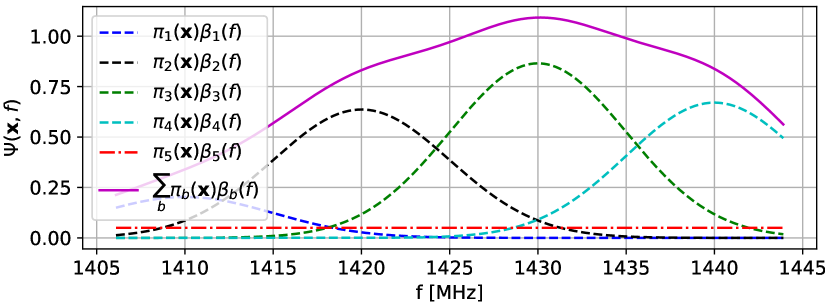
Figure 3: PSD ${\color[rgb]{0,0,0}\Psi}(\bm{x},f)$ at location $\bm{x}$ using a basis expansion model with Gaussian functions.

Under a basis expansion model, the transmit PSD of each source is expressed as

$${{\color[rgb]{0,0,0}\Upsilon}}_{{{\color[rgb]{0,0,0}s}}}(f)=\textstyle\sum_{{{\color[rgb]{0,0,0}b}}=1}^{{{\color[rgb]{0,0,0}B}}-1}{{\color[rgb]{0,0,0}\pi}}_{{{\color[rgb]{0,0,0}s}}{{\color[rgb]{0,0,0}b}}}{{\color[rgb]{0,0,0}\beta}}_{{{\color[rgb]{0,0,0}b}}}(f),$$ (5)

where ${{\color[rgb]{0,0,0}\pi}}_{{{\color[rgb]{0,0,0}s}}{{\color[rgb]{0,0,0}b}}}$ denotes the expansion coefficients and $\{{{\color[rgb]{0,0,0}\beta}}_{{{\color[rgb]{0,0,0}b}}}(f)\}_{{{\color[rgb]{0,0,0}b}}=1}^{{{\color[rgb]{0,0,0}B}}-1}$ is a collection of ${{\color[rgb]{0,0,0}B}}-1$ given basis functions such as raised-cosine or Gaussian functions. Without loss of generality, the basis functions are normalized so that $\int_{-\infty}^{\infty}{{\color[rgb]{0,0,0}\beta}}_{{{\color[rgb]{0,0,0}b}}}(f)df=1$. In this way, if ${{\color[rgb]{0,0,0}\beta}}_{{{\color[rgb]{0,0,0}b}}}(f)$ is the PSD of the ${{\color[rgb]{0,0,0}b}}$-th channel, as possibly specified by a standard, then ${{\color[rgb]{0,0,0}\pi}}_{{{\color[rgb]{0,0,0}s}}{{\color[rgb]{0,0,0}b}}}$ denotes the power transmitted by the ${{\color[rgb]{0,0,0}s}}$-th source in the ${{\color[rgb]{0,0,0}b}}$-th channel. Substituting (5) into (1), the PSD at $\bm{x}\in\mathcal{X}$ reads as

$${\color[rgb]{0,0,0}\Psi}(\bm{x},f) =\sum_{{{\color[rgb]{0,0,0}s}}=1}^{{{\color[rgb]{0,0,0}S}}}\sum_{{{\color[rgb]{0,0,0}b}}=1}^{{{\color[rgb]{0,0,0}B}}-1}{{\color[rgb]{0,0,0}\pi}}_{{{\color[rgb]{0,0,0}s}}{{\color[rgb]{0,0,0}b}}}{{\color[rgb]{0,0,0}\beta}}_{{{\color[rgb]{0,0,0}b}}}(f)|H_{{{\color[rgb]{0,0,0}s}}}(\bm{x},f)|^{2}+\upsilon(\bm{x},f).$$

Now assume that $|H_{{{\color[rgb]{0,0,0}s}}}(\bm{x},f)|^{2}$ remains approximately constant over the support of each basis function, i.e., $|H_{{{\color[rgb]{0,0,0}s}}}(\bm{x},f)|^{2}\approx|H_{{{\color[rgb]{0,0,0}s}}{{\color[rgb]{0,0,0}b}}}(\bm{x})|^{2}$ for all $f$ in the support of ${{\color[rgb]{0,0,0}\beta}}_{{{\color[rgb]{0,0,0}b}}}(f)$. This is a reasonable assumption for narrowband ${{\color[rgb]{0,0,0}\beta}}_{{{\color[rgb]{0,0,0}b}}}(f)$; if it does not hold, one can always split ${{\color[rgb]{0,0,0}\beta}}_{{{\color[rgb]{0,0,0}b}}}(f)$ into multiple basis functions with a smaller frequency support until the assumption holds. Then, the PSD at $\bm{x}$ can be written as

$${\color[rgb]{0,0,0}\Psi}(\bm{x},f)=\sum_{{{\color[rgb]{0,0,0}b}}=1}^{{{\color[rgb]{0,0,0}B}}-1}{{\color[rgb]{0,0,0}\pi}}_{{{\color[rgb]{0,0,0}b}}}(\bm{x}){{\color[rgb]{0,0,0}\beta}}_{{{\color[rgb]{0,0,0}b}}}(f)+\upsilon(\bm{x},f),$$ (6)

where ${{\color[rgb]{0,0,0}\pi}}_{{{\color[rgb]{0,0,0}b}}}(\bm{x}){:=}\textstyle\sum_{{{\color[rgb]{0,0,0}s}}=1}^{{{\color[rgb]{0,0,0}S}}}{{\color[rgb]{0,0,0}\pi}}_{{{\color[rgb]{0,0,0}s}}{{\color[rgb]{0,0,0}b}}}|H_{{{\color[rgb]{0,0,0}s}}{{\color[rgb]{0,0,0}b}}}(\bm{x})|^{2}$. If ${{\color[rgb]{0,0,0}\beta}}_{{{\color[rgb]{0,0,0}b}}}(f)$ models the transmit PSD of the ${{\color[rgb]{0,0,0}b}}$-th channel, then ${{\color[rgb]{0,0,0}\pi}}_{{{\color[rgb]{0,0,0}b}}}(\bm{x})$ corresponds to the power of the ${{\color[rgb]{0,0,0}b}}$-th channel at $\bm{x}$.

Observe that the noise PSD $\upsilon(\bm{x},f)$ can be similarly expressed in terms of a basis expansion. To simplify the exposition, suppose that $\upsilon(\bm{x},f)$ is expanded with a single term as $\upsilon(\bm{x},f)\approx{{\color[rgb]{0,0,0}\pi}}_{{{\color[rgb]{0,0,0}B}}}(\bm{x}){{\color[rgb]{0,0,0}\beta}}_{{\color[rgb]{0,0,0}B}}(f)$, which in turn implies that (6) becomes

$${\color[rgb]{0,0,0}\Psi}(\bm{x},f)=\sum_{{{\color[rgb]{0,0,0}b}}=1}^{{{\color[rgb]{0,0,0}B}}}{{\color[rgb]{0,0,0}\pi}}_{{{\color[rgb]{0,0,0}b}}}(\bm{x}){{\color[rgb]{0,0,0}\beta}}_{{{\color[rgb]{0,0,0}b}}}(f).$$ (7)

Fig. 3 illustrates this expansion for ${{\color[rgb]{0,0,0}B}}=5$ when $\{{{\color[rgb]{0,0,0}\beta}}_{{\color[rgb]{0,0,0}b}}(f)\}_{{{\color[rgb]{0,0,0}b}}=1}^{4}$ are Gaussian radial basis functions and ${{\color[rgb]{0,0,0}\beta}}_{5}(f)$ is set to be constant to model the PSD of white noise. Note that the adopted basis expansion furthermore allows estimation of the noise power ${{\color[rgb]{0,0,0}\pi}}_{{{\color[rgb]{0,0,0}B}}}(\bm{x})$ at every location. This is of special interest in applications such as cognitive radio [53].

With the above expansion, the tensor $\bm{{\color[rgb]{0,0,0}\Psi}}\in\mathbb{R}^{N_{y}\times N_{x}\times N_{f}}$ introduced in Sec. III-A can be expressed as $\left[\bm{{\color[rgb]{0,0,0}\Psi}}\right]_{i,j,n_{f}}=\sum_{{{\color[rgb]{0,0,0}b}}=1}^{{{\color[rgb]{0,0,0}B}}}{{\color[rgb]{0,0,0}\bm{\Pi}}}_{i,j,{{\color[rgb]{0,0,0}b}}}{{\color[rgb]{0,0,0}\beta}}_{{{\color[rgb]{0,0,0}b}}}(f_{n_{f}})$, where ${{\color[rgb]{0,0,0}\bm{\Pi}}}\in\mathbb{R}^{N_{y}\times N_{x}\times{{\color[rgb]{0,0,0}B}}}$ contains the coefficients $\left[{{\color[rgb]{0,0,0}\bm{\Pi}}}\right]_{i,j,{{\color[rgb]{0,0,0}b}}}={{\color[rgb]{0,0,0}\pi}}_{{{\color[rgb]{0,0,0}b}}}({{\color[rgb]{0,0,0}\bm{\xi}}}_{i,j})$. In a deep neural network, this structure can be naturally enforced by setting all but the last layer to obtain an estimate ${{\color[rgb]{0,0,0}{\hat{\bm{\Pi}}}}}$ of ${{\color[rgb]{0,0,0}\bm{\Pi}}}$ and the last layer to produce ${{\color[rgb]{0,0,0}{\hat{\bm{{\color[rgb]{0,0,0}\Psi}}}}}}$. Specifically, the neural network can be expressed schematically as:

$$\begin{aligned} &\mathcal{L}&\overset{{\color[rgb]{0,0,0}\bar{p}_{\bm{w}}}}{\xrightarrow{\hskip 19.91684pt}}&\quad\mathbb{R}^{N_{y}\times N_{x}\times{{\color[rgb]{0,0,0}B}}}&\overset{{\color[rgb]{0,0,0}p}^{{\color[rgb]{0,0,0}(}{\color[rgb]{0,0,0}L}{\color[rgb]{0,0,0})}}}{\xrightarrow{\hskip 19.91684pt}}&\quad\mathbb{R}^{N_{y}\times N_{x}\times N_{f}}\\ &{{\color[rgb]{0,0,0}{\color[rgb]{0,0,0}\breve{\bm{\Psi}}}}}&\xrightarrow{\hskip 19.91684pt}&\quad{{\color[rgb]{0,0,0}{\hat{\bm{\Pi}}}}}&\xrightarrow{\hskip 19.91684pt}&\quad{{\color[rgb]{0,0,0}{\hat{\bm{{\color[rgb]{0,0,0}\Psi}}}}}},\end{aligned}$$

where $\mathcal{L}\subset\mathbb{R}^{N_{y}\times N_{x}\times(N_{f}+N_{m})}$ is the input space, function ${\color[rgb]{0,0,0}\bar{p}_{\bm{w}}}({{\color[rgb]{0,0,0}{\color[rgb]{0,0,0}\breve{\bm{\Psi}}}}}){:=}{\color[rgb]{0,0,0}p}^{{\color[rgb]{0,0,0}(}{\color[rgb]{0,0,0}L}-1{\color[rgb]{0,0,0})}}_{\bm{w}_{{\color[rgb]{0,0,0}L}-1}}(\ldots{\color[rgb]{0,0,0}p}^{{\color[rgb]{0,0,0}(}1{\color[rgb]{0,0,0})}}_{\bm{w}_{1}}({{\color[rgb]{0,0,0}{\color[rgb]{0,0,0}\breve{\bm{\Psi}}}}}))$ groups the first ${\color[rgb]{0,0,0}L}-1$ layers, and ${\color[rgb]{0,0,0}p}^{{\color[rgb]{0,0,0}(}{\color[rgb]{0,0,0}L}{\color[rgb]{0,0,0})}}$ denotes the last layer. With this notation, ${{\color[rgb]{0,0,0}{\hat{\bm{\Pi}}}}}={\color[rgb]{0,0,0}\bar{p}_{\bm{w}}}(\bm{{{\color[rgb]{0,0,0}{\color[rgb]{0,0,0}\breve{\bm{\Psi}}}}}})$ and ${{\color[rgb]{0,0,0}{\hat{\bm{{\color[rgb]{0,0,0}\Psi}}}}}}={\color[rgb]{0,0,0}p}^{{\color[rgb]{0,0,0}(}{\color[rgb]{0,0,0}L}{\color[rgb]{0,0,0})}}({{\color[rgb]{0,0,0}{\hat{\bm{\Pi}}}}})\in\mathbb{R}^{N_{y}\times N_{x}\times N_{f}}$, where $[{{\color[rgb]{0,0,0}{\hat{\bm{{\color[rgb]{0,0,0}\Psi}}}}}}]_{i,j,n_{f}}=\sum_{{{\color[rgb]{0,0,0}b}}=1}^{{{\color[rgb]{0,0,0}B}}}{{\color[rgb]{0,0,0}{\hat{\bm{\Pi}}}}}_{i,j,{{\color[rgb]{0,0,0}b}}}{{\color[rgb]{0,0,0}\beta}}_{{{\color[rgb]{0,0,0}b}}}(f_{n_{f}})$. Observe that, as reflected by the notation, the last layer ${\color[rgb]{0,0,0}p}^{{\color[rgb]{0,0,0}(}{\color[rgb]{0,0,0}L}{\color[rgb]{0,0,0})}}$ does not involve trainable parameters. Furthermore, notice that the number of neurons in the last trainable layer has been reduced from $N_{y}N_{x}N_{f}$ to $N_{y}N_{x}{{\color[rgb]{0,0,0}B}}$.

To sum up, this section presented two possibilities to reduce the number of parameters of the network, which can improve estimation performance for a given training size. Whereas the approach in Sec. III-C1 is more suitable for narrowband channels, the approach in Sec. III-C2 lends itself to wideband communications, where propagation effects may significantly differ across frequencies.

III-D Deep Completion Autoencoders

The previous section addressed design aspects pertaining to the map structure in the frequency domain. In contrast, this section deals with structure across space. In particular, a deep neural network architecture based on fully convolutional autoencoders [54] will be developed.

A (conventional) autoencoder [46, Ch. 12] is a neural network ${\color[rgb]{0,0,0}p_{\bm{w}}}$ that can be expressed as the composition of a function ${\color[rgb]{0,0,0}\epsilon}_{{\color[rgb]{0,0,0}\bm{w}}}$ termed encoder and a function ${\color[rgb]{0,0,0}\delta}_{{\color[rgb]{0,0,0}\bm{w}}}$ called decoder, i.e., ${\color[rgb]{0,0,0}p_{\bm{w}}}({{\color[rgb]{0,0,0}\bm{\Phi}}})={\color[rgb]{0,0,0}\delta}_{{\color[rgb]{0,0,0}\bm{w}}}({\color[rgb]{0,0,0}\epsilon}_{{\color[rgb]{0,0,0}\bm{w}}}({{\color[rgb]{0,0,0}\bm{\Phi}}}))~{}\forall{{\color[rgb]{0,0,0}\bm{\Phi}}}$. The output of the encoder ${\color[rgb]{0,0,0}\bm{\lambda}}{:=}{\color[rgb]{0,0,0}\epsilon}_{{\color[rgb]{0,0,0}\bm{w}}}({{\color[rgb]{0,0,0}\bm{\Phi}}})\in\mathbb{R}^{{\color[rgb]{0,0,0}N_{\lambda}}}$ is referred to as the code or vector of latent variables and is of a typically much lower dimension than the input ${{\color[rgb]{0,0,0}\bm{\Phi}}}$. An autoencoder is trained so that ${\color[rgb]{0,0,0}\delta}_{{\color[rgb]{0,0,0}\bm{w}}}({\color[rgb]{0,0,0}\epsilon}_{{\color[rgb]{0,0,0}\bm{w}}}({{\color[rgb]{0,0,0}\bm{\Phi}}}))\approx{{\color[rgb]{0,0,0}\bm{\Phi}}}~{}\forall{{\color[rgb]{0,0,0}\bm{\Phi}}}$, which forces the encoder to compress the information in ${{\color[rgb]{0,0,0}\bm{\Phi}}}$ into the ${\color[rgb]{0,0,0}N_{\lambda}}$ variables in ${\color[rgb]{0,0,0}\bm{\lambda}}$.

A completion autoencoder adheres to the same principles as conventional autoencoders except for the fact that the encoder must determine the latent variables from a subset of the entries of the input. If a mask is used, then ${{\color[rgb]{0,0,0}\bm{\Phi}}}\approx{\color[rgb]{0,0,0}\delta}_{{\color[rgb]{0,0,0}\bm{w}}}({\color[rgb]{0,0,0}\epsilon}_{{\color[rgb]{0,0,0}\bm{w}}}(\mathcal{P}_{\Omega}({{\color[rgb]{0,0,0}\bm{\Phi}}}),\bm{{\color[rgb]{0,0,0}M}}_{\Omega}))~{}\forall{{\color[rgb]{0,0,0}\bm{\Phi}}}$ if the sampling set $\Omega$ preserves sufficient information for reconstruction – if $\Omega$ does not satisfy this requirement, then reconstructing ${{\color[rgb]{0,0,0}\bm{\Phi}}}$ is impossible regardless of the technique used. In the application at hand and with the notation introduced in previous sections, the above expression becomes $\mathcal{P}_{\Omega}({{\tilde{\bm{{\color[rgb]{0,0,0}\Psi}}}}})\approx\mathcal{P}_{\Omega}({\color[rgb]{0,0,0}\delta}_{{\color[rgb]{0,0,0}\bm{w}}}({\color[rgb]{0,0,0}\epsilon}_{{\color[rgb]{0,0,0}\bm{w}}}({{\color[rgb]{0,0,0}{\color[rgb]{0,0,0}\breve{\bm{\Psi}}}}})))$.

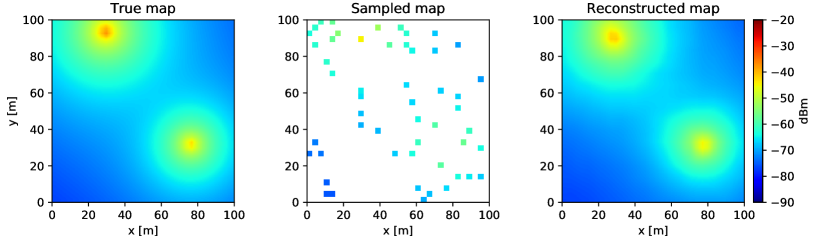
Figure 4: Estimation with $N_{\lambda}=4$ latent variables: (left) true map, (middle) sampled map portraying grid points $\{{{\color[rgb]{0,0,0}\bm{\xi}}}_{i,j}\}$ with $|\mathcal{A}_{i,j}|>0$, and (right) map estimate.

As indicated earlier, autoencoders are useful only when most of the information in the input can be condensed in ${\color[rgb]{0,0,0}N_{\lambda}}$ variables, i.e., when the possible inputs lie close to a manifold of dimension ${\color[rgb]{0,0,0}N_{\lambda}}$. To see that this is indeed the case in radio map estimation, an illustrating toy example is presented next. Consider two sources transmitting with a different but fixed power at arbitrary positions in $\mathcal{X}$ and suppose that propagation occurs in free space. All possible spectrum maps in this setup can therefore be uniquely identified by ${\color[rgb]{0,0,0}N_{\lambda}}=4$ quantities, namely the x and y coordinates of the two sources. Fig. 4 illustrates this effect, where the left panel of Fig. 4 depicts a true map $\bm{{\color[rgb]{0,0,0}\Psi}}$ and the right panel shows its estimate using the proposed completion autoencoder when ${\color[rgb]{0,0,0}N_{\lambda}}=4$. Although the details about the network and simulation setup are deferred to Sec. IV, one can already notice at this point the quality of the estimate, which clearly supports the aforementioned manifold hypothesis. In a real-world scenario, there may be more than two sources, their transmit power may not always be the same, and there are shadowing effects, which means that ${\color[rgb]{0,0,0}N_{\lambda}}\geq 4$ will be generally required.

The rest of this section will describe the main aspects of the architecture developed in this work and summarized in Fig. 5. The main design decisions are supported here by arguments and intuition. Empirical support is provided in Sec. IV-B.

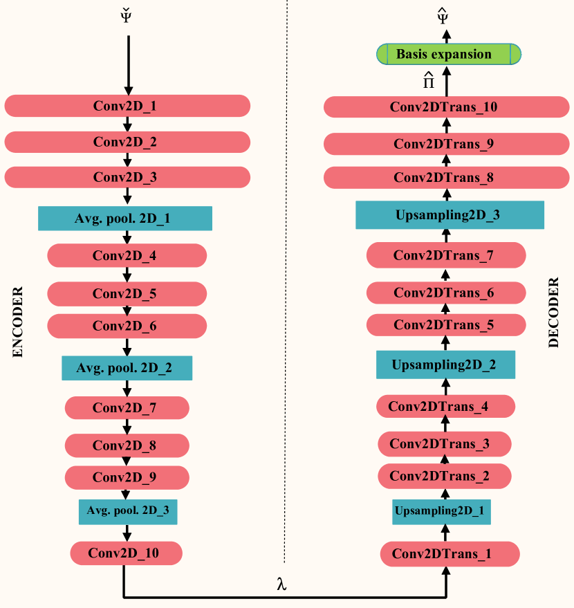
Figure 5: Autoencoder architecture.

The encoder mainly comprises convolutional and pooling layers. The motivation for convolutional layers is three-fold: (i) relative to fully connected layers, they severely reduce the number of parameters to train and, consequently, the amount of data required. Despite this drastic reduction, (ii) convolutional layers are still capable of exploiting the spatial structure of maps and (iii) they result in shift-invariant transfer functions, a desirable property in the application at hand since moving the sources in a certain direction must be corresponded by the same movement in the map estimate. Recall that a convolutional layer with input ${{\color[rgb]{0,0,0}\bm{\Phi}}}^{(I)}$ and output ${{\color[rgb]{0,0,0}\bm{\Phi}}}^{(O)}$ linearly combines 2D convolutions as

$$[{{\color[rgb]{0,0,0}\bm{\Phi}}}^{(O)}]_{i,j,{{\color[rgb]{0,0,0}c_{\text{out}}}}}=\sum_{{{\color[rgb]{0,0,0}c_{\text{in}}}}=1}^{{\color[rgb]{0,0,0}C_{\text{in}}}}\sum_{u=-k}^{k}\sum_{v=-k}^{k}[\bm{F}_{{\color[rgb]{0,0,0}c_{\text{out}}}}]_{u,v,{{\color[rgb]{0,0,0}c_{\text{in}}}}}[{{\color[rgb]{0,0,0}\bm{\Phi}}}^{(I)}]_{i-u,j-v,{{\color[rgb]{0,0,0}c_{\text{in}}}}},$$ (8)

where the ${{\color[rgb]{0,0,0}c_{\text{out}}}}$-th kernel $\bm{F}_{{\color[rgb]{0,0,0}c_{\text{out}}}}$ is of size $2k+1\times 2k+1\times{{\color[rgb]{0,0,0}C_{\text{in}}}}$. Layer indices were omitted in order not to overload notation. The adopted activation functions are parametric leaky rectified linear units (PReLUs) [55], whose leaky parameter is also trained; see also Sec. IV-B. Average pooling layers are used to down-sample the outputs of convolutional layers, thereby condensing the information gradually in fewer features while approximately preserving shift invariance [46, Ch. 9].

As usual in autoencoders, the decoder follows a “reverse” architecture relative to the encoder. Specifically, for each convolutional layer of the encoder, the decoder has a corresponding  convolution transpose layer [56], sometimes called “deconvolutional” layer. Likewise, the pooling layers of the encoder are matched with up-sampling layers. A simple possibility is to implement such an upsampling operation by means of bilinear interpolation. Alternatively, one can replace a convolution transpose layer followed by an interpolation layer with a single convolution layer with a fractional stride [56].

TABLE I: Parameters of the proposed network.

Layers	Parameters
Conv2D/ Conv2DTranspose	Kernel size = $3\times 3$, stride = 1, activation = PLReLU, 32 filters
AveragePooling2D	Pool size = 2, stride = 2
Upsampling2D	Up-sampling factor = $2$, bilinear interpolation

Observe that the proposed network, summarized in Fig. 5 and Table I, is fully convolutional, which means that there are no fully connected layers. This not only leads to a better estimation performance due to the reduced number of parameters to train (cf. Sec. IV), but also enables the possibility of utilizing the same network with any value of $N_{x}$ and $N_{y}$. With fully connected layers, one would generally require a different network for each pair $(N_{x},N_{y})$, which would clearly have negative implications for training.

The computational complexity of the proposed network when estimating a radio map is clearly given by the computational complexity of a forward pass. The latter is dominated by the complexity of the convolutional layers, which, from (8), can be seen to involve $\sum_{\tilde{l}=1}^{\tilde{L}}(2k_{\tilde{l}}+1)^{2}C_{\text{in},\tilde{l}}C_{\text{out},\tilde{l}}N_{x,\tilde{l}}N_{y,\tilde{l}}$ products in total, where $\tilde{l}$ indexes the $\tilde{L}$ convolutional layers, $k_{\tilde{l}}$ and $C_{\text{in},\tilde{l}}$ are such that the kernel of the $\tilde{l}$-th layer is of size $(2k_{\tilde{l}}+1)\times(2k_{\tilde{l}}+1)\times C_{\text{in},\tilde{l}}$, whereas $N_{x,\tilde{l}}$, $N_{y,\tilde{l}}$, and $C_{\text{out},\tilde{l}}$ are such that the output of the $\tilde{l}$-th layer is $N_{x,\tilde{l}}\times N_{y,\tilde{l}}\times C_{\text{out},\tilde{l}}$. Note that these constants are determined by the strides, intermediate pooling layers, and the adopted padding technique.

III-E Learning in Real-World Scenarios

A key novelty in this paper is to obtain map estimators by learning from data. This section describes how to construct a suitable training set in the application at hand. Specifically, three approaches are discussed:

III-E1 Synthetic Training Data

Since collecting a large number of training maps may be slow or expensive, one can instead generate maps using a mathematical model or simulator that captures the structure of the propagation phenomena, such as path loss and shadowing; see e.g. [57]. Fitting ${\color[rgb]{0,0,0}p_{\bm{w}}}$ to data generated by that model would, in principle, yield an estimator that effectively exploits this structure. The idea is, therefore, to generate $T$ maps $\{{\color[rgb]{0,0,0}\Psi}_{t}(\bm{x},f)\}_{t=1}^{T}$ together with $T$ sampling sets $\{\Omega_{t}\}_{t=1}^{T}$. Afterwards, $\{{{\tilde{\bm{{\color[rgb]{0,0,0}\Psi}}}}}_{t}\}_{t=1}^{T}$ and $\{{{\color[rgb]{0,0,0}{\color[rgb]{0,0,0}\breve{\bm{\Psi}}}}}_{t}\}_{t=1}^{T}$ can be formed as described earlier. It is possible to add artificially generated noise to the synthetic measurements in ${{\tilde{\bm{{\color[rgb]{0,0,0}\Psi}}}}}_{t}$ to model the effect of measurement error. This would train the network to counteract the impact of such error, along the lines of denoising autoencoders [46, Ch. 14].

The advantage of this approach is that one has access to the ground truth, i.e., one can use the true maps $\bm{{\color[rgb]{0,0,0}\Psi}}_{t}$ as targets. Specifically, the neural network can be trained on the data $\{({{\color[rgb]{0,0,0}{\color[rgb]{0,0,0}\breve{\bm{\Psi}}}}}_{t},\bm{{\color[rgb]{0,0,0}\Psi}}_{t})\}_{t=1}^{T}$ by solving

$$\mathop{\text{minimize}}_{~{}\bm{w}}\quad\frac{1}{T}\sum_{t=1}^{T}\left\|\bm{{\color[rgb]{0,0,0}\Psi}}_{t}-p_{\bm{w}}({{\color[rgb]{0,0,0}{\color[rgb]{0,0,0}\breve{\bm{\Psi}}}}}_{t})\right\|_{F}^{2}.$$ (9)

If the model or simulator is sufficiently close to the reality, completing a real-world map ${{\color[rgb]{0,0,0}{\color[rgb]{0,0,0}\breve{\bm{\Psi}}}}}$ as ${\color[rgb]{0,0,0}p_{\bm{w}}}({{\color[rgb]{0,0,0}{\color[rgb]{0,0,0}\breve{\bm{\Psi}}}}})$ should produce an accurate estimate.

III-E2 Real Training Data

In practice, real maps may be available for training. However, in most cases, it will not be possible to collect measurements at all grid points within a sufficiently short time interval; see Remark 2. Besides, it is not possible to obtain the entries of $\bm{{\color[rgb]{0,0,0}\Psi}}$ but only measurements of it. This means that a real training set comprises tensors $\{{{\color[rgb]{0,0,0}{\color[rgb]{0,0,0}\breve{\bm{\Psi}}}}}_{t},~{}t=1,\ldots,T\}$ but not $\bm{{\color[rgb]{0,0,0}\Psi}}_{t}$.

For training, one can plug this data directly into (3) or (4). However, ${\color[rgb]{0,0,0}p_{\bm{w}}}$ may then learn to fit just the observed entries $\{[{{\tilde{\bm{{\color[rgb]{0,0,0}\Psi}}}}}_{t}(f)]_{i,j},~{}(i,j)\in\Omega_{t}\}$, as would happen e.g. when ${\color[rgb]{0,0,0}p_{\bm{w}}}$ is the identity mapping. To counteract this trend, one can adopt a sufficiently small ${\color[rgb]{0,0,0}N_{\lambda}}$. The downside is that estimation performance may be damaged. To bypass this difficulty, the approach proposed here is to use part of the measurements as the input and another part as the output (target). Specifically, for each $t$, construct $Q_{t}$ pairs of (not necessarily disjoint) subsets $\Omega_{t,q}^{(I)},\Omega_{t,q}^{(O)}\subset\Omega_{t}$, $q=1,\ldots,Q_{t}$, e.g by drawing a given number of elements of $\Omega_{t}$ uniformly at random without replacement. Using these subsets, subsample ${{\tilde{\bm{{\color[rgb]{0,0,0}\Psi}}}}}_{t}$ to yield ${{\tilde{\bm{{\color[rgb]{0,0,0}\Psi}}}}}_{t,q}^{(I)}{:=}\mathcal{P}_{\Omega^{(I)}_{t,q}}({{\tilde{\bm{{\color[rgb]{0,0,0}\Psi}}}}}_{t})$ and ${{\tilde{\bm{{\color[rgb]{0,0,0}\Psi}}}}}_{t,q}^{(O)}{:=}\mathcal{P}_{\Omega^{(O)}_{t,q}}({{\tilde{\bm{{\color[rgb]{0,0,0}\Psi}}}}}_{t})$. With the resulting $\sum_{t}Q_{t}$ training instances, one can think of solving

$$\begin{split}\mathop{\text{minimize}}_{\bm{w}}&\textstyle\quad\frac{1}{\sum_{t}Q_{t}}\sum_{t=1}^{T}\sum_{q=1}^{Q_{t}}\\ &\left\|\mathcal{P}_{\Omega_{t,q}^{(O)}}\left(\tilde{\bm{{\color[rgb]{0,0,0}\Psi}}}_{t,q}^{(O)}-p_{\bm{w}}\left({{\color[rgb]{0,0,0}{\color[rgb]{0,0,0}\breve{\bm{\Psi}}}}}_{t,q}^{(I)}\right)\right)\right\|_{F}^{2},\end{split}$$ (10)

where ${{\color[rgb]{0,0,0}{\color[rgb]{0,0,0}\breve{\bm{\Psi}}}}}_{t,q}^{(I)}$ is formed by concatenating $\tilde{\bm{{\color[rgb]{0,0,0}\Psi}}}_{t,q}^{(I)}$ and $\bm{{\color[rgb]{0,0,0}M}}_{\Omega_{t,q}^{(I)}}$.

III-E3 Hybrid Training

In practice, one expects to have real data, but only in a limited amount. It then makes sense to apply the notion of transfer learning [46, Ch. 15] as follows: first, learn an initial parameter vector $\bm{w}^{*}$ by solving (9) with synthetic data. Second, solve (10) with real data, but using $\bm{w}^{*}$ as initialization for the optimization algorithm. The impact of choosing this initialization is that the result of solving (10) in the second step will be generally closer to a “better” local optimum than if a random initialization were adopted. Hence, this approach combines the information of both synthetic and real data sets.

IV Numerical Experiments

This section validates the proposed framework and network architecture through numerical experiments.

Unless stated otherwise, the region of interest $\mathcal{X}$ is a square area of side $100$ m, discretized into a grid with $N_{y}=N_{x}=32$. Two data sets are constructed as described next. First, $T=5\cdot 10^{5}$ maps are generated where the two considered transmitters are placed uniformly at random in $\mathcal{X}$, have height 1.5 m, and transmit with power in each channel drawn uniformly at random between $5$ and $11$ dBm. The pathloss exponent is set to 3, whereas the gain at unit distance is $-30$ dB. The lognormal shadowing component adheres to the Gudmundson model [58], which provides the correlation between the shadowing of two links that share an endpoint. Specifically, in this paper, $\mathop{\textrm{E}}\left\{H_{{\color[rgb]{0,0,0}s}}(\bm{x}_{1},f)H_{{\color[rgb]{0,0,0}s}}(\bm{x}_{2},f)\right\}=\sigma_{\text{sh}}^{2}0.95^{||\bm{x}_{1}-\bm{x}_{2}||}$, where $\sigma_{\text{sh}}^{2}=10$ dB² and $||\bm{x}_{1}-\bm{x}_{2}||$ is the distance between $\bm{x}_{1}$ and $\bm{x}_{2}$ in meters. Measurement locations are drawn uniformly at random without replacement across the grid points. Each measurement ${{\color[rgb]{0,0,0}\tilde{\color[rgb]{0,0,0}\Psi}}}(\bm{x}_{n},f)$ is obtained by adding zero-mean Gaussian noise with standard deviation 1 dB to ${\color[rgb]{0,0,0}\Psi}(\bm{x}_{n},f)$.

A second data set of $T=1.25\cdot 10^{5}$ maps is generated using Remcom’s Wireless InSite software in the “urban canyon” scenario, where a pair of transmitters are deployed per map in the downtown of Rosslyn, Virginia. The area is a square of approximately 700 m side, out of which $N_{x}\times N_{y}$ patches are generated by drawing the coordinates of their bottom-left corner uniformly at random. The ray tracing (RT) algorithm used there in combination with a 3D map of the city is based on the shooting and bouncing ray method [59] (see also [60, Ch. 8]) with the maximum number of reflections and diffractions set to 6 and 2, respectively. This data set can be regarded as a realistic surrogate of a data set with real measurements due to the solid theoretical foundations of RT algorithms on Maxwell’s equations. Besides, they are extensively employed to construct data sets in related works [20, 21, 25, 24, 23]. Measurement locations are distributed uniformly at random without replacement across the grid points that lie on the streets. To average out multipath fading present in the generated maps (see Remark 1), ${\color[rgb]{0,0,0}\Psi}({{\color[rgb]{0,0,0}\bm{\xi}}}_{i,j},f)$ is replaced with $({1}/{|\mathcal{N}_{i,j}|)}\sum_{{{\color[rgb]{0,0,0}\bm{\xi}}}\in\mathcal{N}_{i,j}}{\color[rgb]{0,0,0}\Psi}({{\color[rgb]{0,0,0}\bm{\xi}}},f)$, where $\mathcal{N}_{i,j}$ contains the $|\mathcal{N}_{i,j}|=9$ grid points that lie closest to ${{\color[rgb]{0,0,0}\bm{\xi}}}_{i,j}$, including ${{\color[rgb]{0,0,0}\bm{\xi}}}_{i,j}$. A binary mask indicating the position of buildings is combined with the sample mask as indicated at the end of Remark 3.

The network proposed in Sec. III-D with code length ${\color[rgb]{0,0,0}N_{\lambda}}=64$ is implemented in TensorFlow and trained using the Adam solver [61] with learning rate $5\cdot 10^{-4}$, batch-size 64, training epochs 100, and the number of measurements $|\Omega_{t}|,~{}t=1,\ldots,T$, in each training map is drawn uniformly at random between 10 and 400. Quantitative evaluation will compare the root mean square error (RMSE), defined as

$$\text{RMSE}=\sqrt{\frac{\mathbb{E}\{||\bm{{\color[rgb]{0,0,0}\Psi}}-\bm{{{\color[rgb]{0,0,0}\hat{\color[rgb]{0,0,0}\Psi}}}}||_{F}^{2}\}}{N_{x}N_{y}N_{f}}},$$ (11)

where $\bm{{\color[rgb]{0,0,0}\Psi}}$ is the true map, $\bm{{{\color[rgb]{0,0,0}\hat{\color[rgb]{0,0,0}\Psi}}}}$ is the map estimate, and $\mathbb{E}\{\cdot\}$ denotes expectation over noise, and sensor locations. The RMSE will be estimated by averaging over a test data set of $10^{3}$ maps.

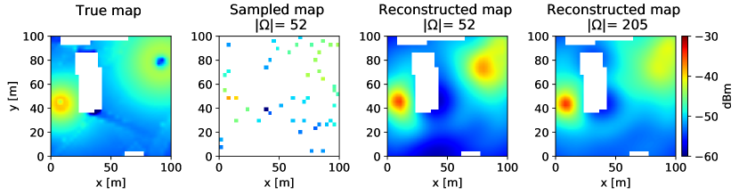
Figure 6: Power map estimate with the proposed neural network. (left): true map, (center left): sampled map portraying the locations of the grid points $\{{{\color[rgb]{0,0,0}\bm{\xi}}}_{i,j}\}$ where $|\mathcal{A}_{i,j}|>0$; (center right) and (right): map estimates for different numbers of measurements $|\Omega|$. White areas represent buildings.

IV-A Power Map Cartography

To analyze the most fundamental radio map estimation aspects, $\mathcal{F}$ is set here to the singleton $\mathcal{F}=\{1400\text{ MHz}\}$ and the bandwidth to 5 MHz in both data sets. To better observe the impact of propagation phenomena, $\upsilon(\bm{x},f)$ is set to 0.

The proposed algorithm is compared against a representative set of competitors, whose parameters were adjusted to approximately yield the best performance. This includes: (i) The kriging algorithm in [2] with regularization parameter $10^{-5}$ and Gaussian radial basis functions with parameter $\sigma_{K}{:=}5\sqrt{{\Delta_{y}N_{y}\Delta_{x}N_{x}}/{|\Omega|}}$, which is approximately 5 times the mean distance between two points at which measurements have been collected. (ii) The multikernel algorithm in [37] with regularization parameter $10^{-4}$ and two kinds of kernels: 20 Laplacian kernels that use a parameter uniformly spaced between $[0.1\sigma_{K},\sigma_{K}]$ and 20 Gaussian kernels that use different parameters between $0.005$ and $100$ m. (iii) Matrix completion via nuclear norm minimization [31] with regularization parameter $10^{-5}$. (iv) Gaussian processes for regression [62, Ch. 5] with regularization parameter $3\cdot 10^{-1}$ and Gaussian radial basis functions. As a benchmark, (v) the $K$-nearest neighbors (KNN) algorithm with $K=5$ is also shown.

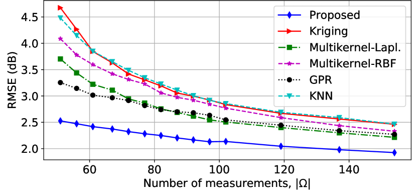
Figure 7: Comparison with state-of-the-art alternatives. Training and testing maps drawn from the Gudmundson data set. The proposed network uses a grid with $N_{y}=N_{x}=64$, two additional Conv2D and Conv2DTranspose layers, code length ${\color[rgb]{0,0,0}N_{\lambda}}=256$, and $T=2.4\cdot 10^{6}$.

IV-A1 Gudmundson Data Set

Performance is assessed next using the training approach in Sec. III-E1 with $\{({{\color[rgb]{0,0,0}{\color[rgb]{0,0,0}\breve{\bm{\Psi}}}}}_{t},\bm{{\color[rgb]{0,0,0}\Psi}}_{t})\}_{t=1}^{T}$ given by the Gudmundson data set.

To analyze estimation of real maps when the proposed network is trained over synthetic data, the first experiment shows two map estimates when the true (test) map is drawn from the Wireless Insite data set. Specifically, the first panel of Fig. 6 depicts the true map, the second shows ${{\tilde{\bm{{\color[rgb]{0,0,0}\Psi}}}}}$, and the remaining two panels show estimates using different numbers of measurements. Observe that with just $|\Omega|=52$ measurements, the estimate is already of a high quality. Note that details due to diffraction, multipath, and antenna directivity are not reconstructed because the Gudmundson data set used to train the network does not capture these effects and, therefore, the network did not learn them.

The second experiment compares the RMSE of the proposed method with that of the competing algorithms. From Fig. 7, the proposed scheme performs approximately a 30 % better than the next competing alternative. Due to the high RMSE of the matrix completion algorithm in [31] for the adopted range of $|\Omega|$ in Fig. 7, its RMSE is not shown in this figure.

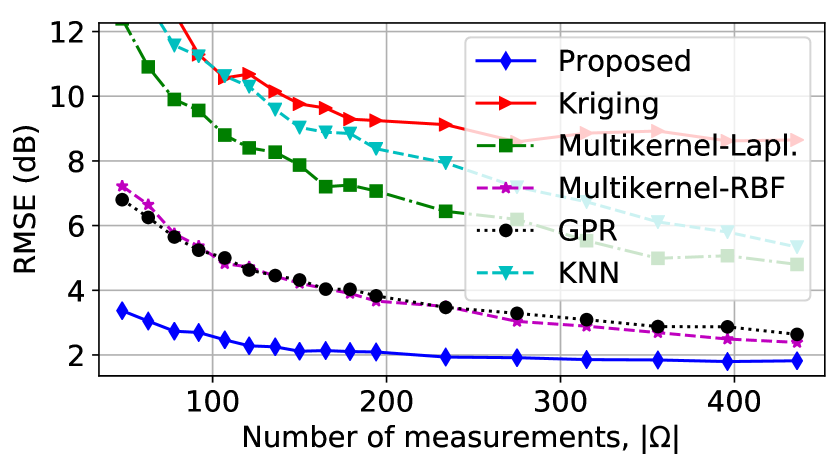
(a)

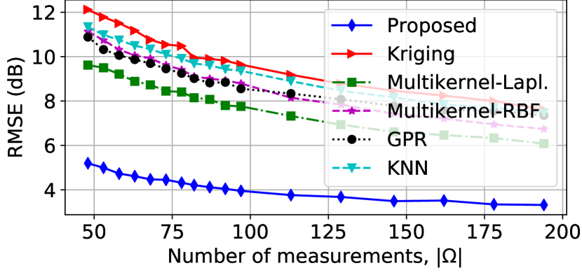
(b)

Figure 8: Comparison with state-of-the-art alternatives when the training and testing maps were obtained from the Wireless InSite data set and $Q_{t}=10$. (a) Square area of side $100$ m with $N_{y}=N_{x}=32$; (b) square area of side $200$ m with $N_{y}=N_{x}=64$. The autoencoder that produces the blue curve in (b) has two additional Conv2D and Conv2DTranspose layers, code length ${\color[rgb]{0,0,0}N_{\lambda}}=256$, and uses $T=1.25\cdot 10^{6}$.

IV-A2 Wireless Insite Data Set

To investigate how the proposed network would perform in a real-world setup, training uses the Wireless Insite data set in combination with the technique in Sec. III-E2, where the sets $\Omega_{t,q}^{(I)}$ and $\Omega_{t,q}^{(O)}$ are drawn from $\Omega_{t}$ uniformly at random without replacement with $|\Omega_{t,q}^{(I)}|=|\Omega_{t,q}^{(O)}|=1/2|\Omega_{t}|$, $q=1,\ldots,Q_{t}$, and $Q_{t}=10~{}\forall t$. Figs. 8a and 8b show the RMSE as a function of $|\Omega|$ for the proposed scheme and competing alternatives with two area sizes. By the performance degradation of all five approaches relative to Fig. 7, it follows that estimating real maps is more challenging than estimating maps in the Gudmundson data set. The performance gap is increased, where the proposed approach now performs roughly 100 and 90 % in Figs. 8a and 8b, respectively, better than the next competing alternative. As in Fig. 7, the algorithm in [31] is not displayed due to a high RMSE.

IV-A3 Hybrid Training

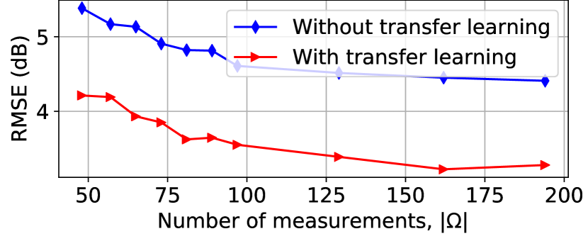
Figure 9: Performance gain due to hybrid training using $T=10^{3}$ maps with $Q_{t}=30$ from the Wireless InSite data set. The initial weights used for the blue curve were drawn at random whereas those for the red curve were obtained by training over the Gudmundson data set.

The performance of the hybrid training scheme from Sec. III-E3 is analyzed in Fig. 9. As expected, transfer learning yields a significant performance improvement.

IV-B Deep Neural Network Design

This section justifies the main design decisions regarding the proposed network. To unveil the influence of each architectural aspect, the number of convolution and convolution-transpose filters is adjusted so that the total number of parameters of the neural network $N_{{\color[rgb]{0,0,0}\bm{w}}}$ remains approximately the same.

The first step is to justify the choice of an autoencoder structure. To this end, Fig. 10 complements the toy example in Fig. 4 by plotting the RMSE as a function of the code length ${\color[rgb]{0,0,0}N_{\lambda}}$ under two setups with pathloss propagation and fixed transmit power: i) Noisy inputs, noiseless targets in the training phase, and noisy inputs, noiseless targets in the testing phase. This corresponds to training as a denoising autoencoder; see Sec. III-E1. ii) Noisy inputs and targets in the training, and noisy inputs, noiseless targets in the testing. This models how a neural network trained over real data estimates a true map. Note that the irregular behavior of the curves for ${\color[rgb]{0,0,0}N_{\lambda}}>5$ owes to the fact that each ${\color[rgb]{0,0,0}N_{\lambda}}$ corresponds to a different network, and therefore a different training process, including the initialization. As observed, the RMSE remains roughly constant for ${\color[rgb]{0,0,0}N_{\lambda}}>5$, which demonstrates that the spectrum maps in this scenario lie close to a low-dimensional manifold. This justifies the autoencoder structure. Besides, training as a denoising autoencoder offers a slight performance advantage, yet it is only possible with synthetic data; see Sec. III-E1. When other propagation phenomena such as shadowing need to be accounted for, ${\color[rgb]{0,0,0}N_{\lambda}}>5$ is however required.

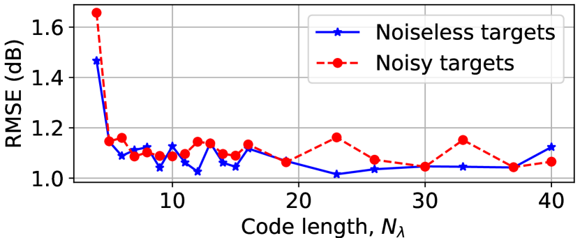
Figure 10: RMSE as a function of the code length ${\color[rgb]{0,0,0}N_{\lambda}}$, $|\Omega|=104$.

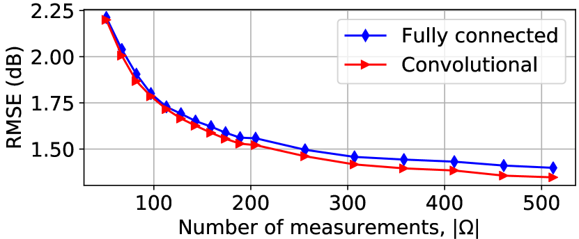
Figure 11: RMSE of the proposed network as a function of $|\Omega|$ for two types of output layers for the encoder.

A second design consideration is whether the last layer of the encoder should be convolutional or fully connected. In the former case, the code would capture shift-invariant features, whereas greater flexibility is allowed in the latter case. This dilemma is ubiquitous in deep learning since convolutional layers constitute a special case of fully connected layers. The decision involves the trade-off between flexibility and information that can be learned with a finite number of training examples. This is investigated in Fig. 11, which shows the RMSE as a function of the number of measurements $|\Omega|$ for these two types of layers. As observed, in the present case, fully convolutional autoencoders perform slightly better. Besides, they accommodate inputs of arbitrary $N_{x}$ and $N_{y}$. For these reasons, the proposed architecture is fully convolutional.

Two more design decisions involve the number of layers ${\color[rgb]{0,0,0}L}$ and the choice of the activation functions. Fig. 12 shows the RMSE as a function of ${\color[rgb]{0,0,0}L}$ with LeakyReLU and PReLU activations [55], where the latter generalize the former to allow training the leaky parameter. Recall that the number of neurons per layer is adjusted to yield approximately the same number of training parameters for all ${\color[rgb]{0,0,0}L}$. Thus, this figure embodies the trade-off between the number and complexity of the features extracted by the network as well as the impact of overfitting. As observed, the best performance in this case is achieved around ${\color[rgb]{0,0,0}L}=26$ layers. Both activations yield roughly the same RMSE, yet the PReLU outperforms the LeakyReLU for shallow architectures.

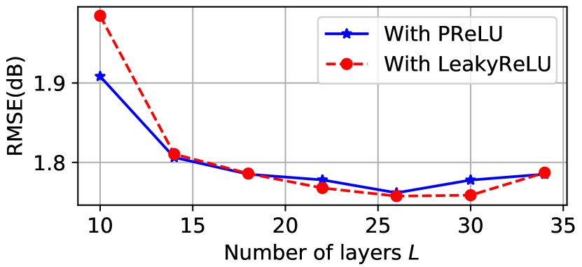
Figure 12: Estimation RMSE of the proposed approach as a function of the number of layers ${\color[rgb]{0,0,0}L}$ of the autoencoder for two different activation functions, $|\Omega|=300$.

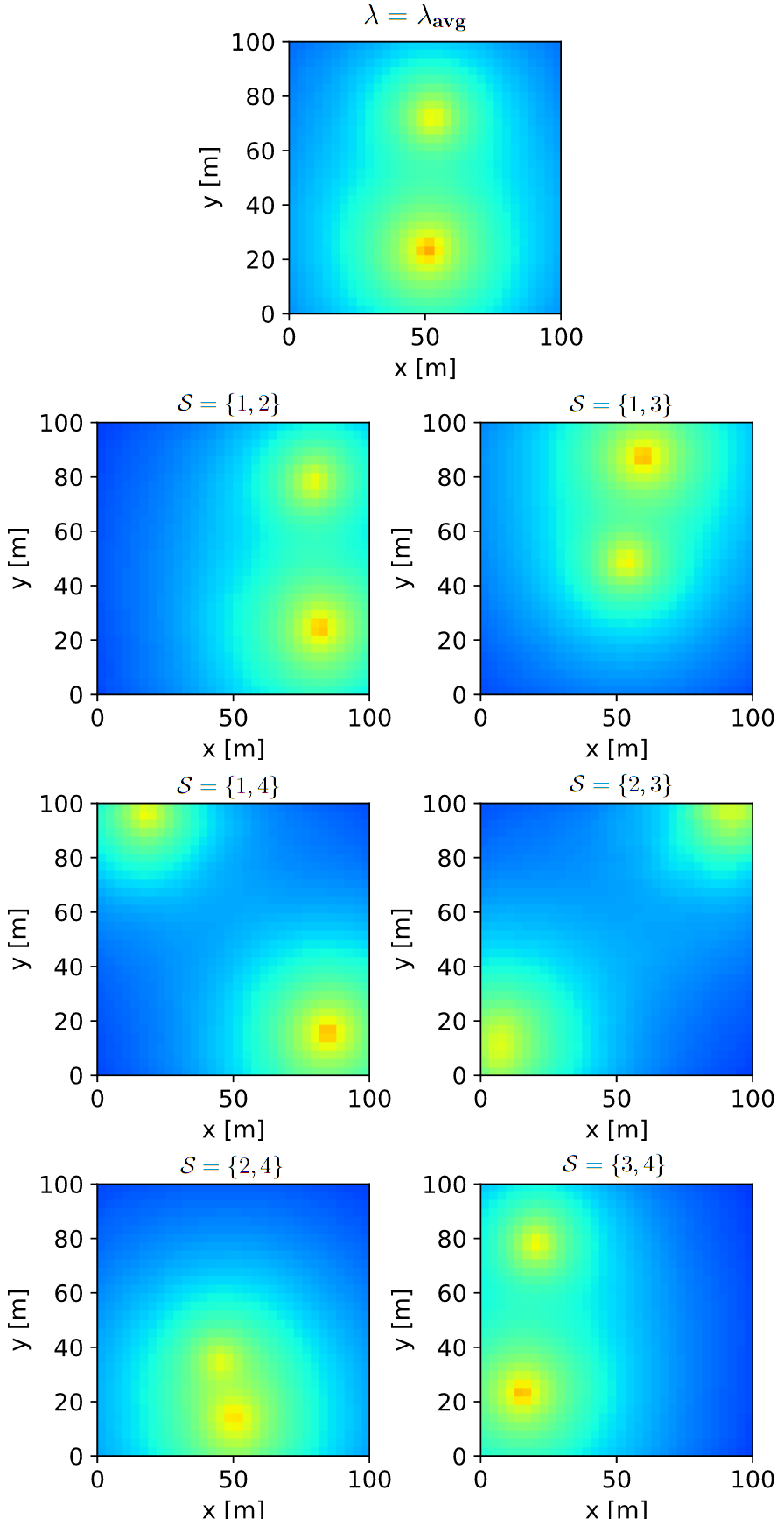
(a)

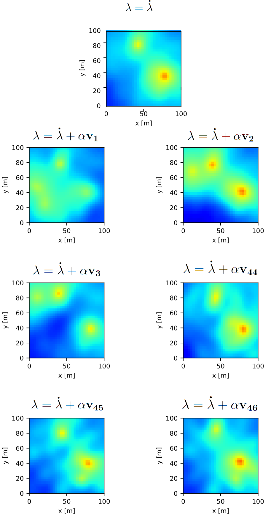
(b)

Figure 13: Decoder outputs of autoencoder architectures with different code length and trained with different data sets: (a) ${\color[rgb]{0,0,0}N_{\lambda}}=4$ with maps from the free-space propagation model, (b) ${\color[rgb]{0,0,0}N_{\lambda}}=64$ with maps from the Gudmundson data set, $\alpha=10$.

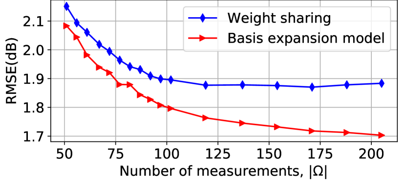
Figure 14: Map estimation RMSE with and without prior information in the frequency domain.

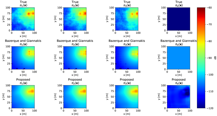
Figure 15: Maps of the true and estimated cofficients $\{{{\color[rgb]{0,0,0}\pi}}_{{\color[rgb]{0,0,0}b}}(\bm{x})\}_{{{\color[rgb]{0,0,0}b}}=1}^{{{\color[rgb]{0,0,0}B}}}$ over $\mathcal{X}$, ${{\color[rgb]{0,0,0}B}}=4$.

IV-C Feature Visualization

Although neural networks are mainly treated as black boxes, some visualization techniques offer interpretability of the features that they extract and, therefore, shed light on the nature of the information that is learned. To this end, the next experiment depicts the decoder output when different latent vectors ${\color[rgb]{0,0,0}\bm{\lambda}}\in\mathbb{R}^{{\color[rgb]{0,0,0}N_{\lambda}}}$ are fed at its input.

First, an instance of the proposed autoencoder with ${\color[rgb]{0,0,0}N_{\lambda}}=4$ is trained with a dataset of $T_{{\color[rgb]{0,0,0}N_{\lambda}}}=3\cdot 10^{3}$ maps generated using the free-space propagation model with two sources transmitting with a fixed power. Since these maps only differ in the x and y coordinates of the sources, they form a $4$-dimensional manifold. Applying the encoder to those maps yields $\{{\color[rgb]{0,0,0}\bm{\lambda}}_{t}\}_{t=1}^{T_{{\color[rgb]{0,0,0}N_{\lambda}}}}$. The top panel of Fig. 13a depicts the output of the trained decoder when ${{\color[rgb]{0,0,0}\bm{\lambda}}}={\color[rgb]{0,0,0}\bm{\lambda}}_{\text{avg}}$, where ${\color[rgb]{0,0,0}\bm{\lambda}}_{\text{avg}}{:=}(1/T_{{\color[rgb]{0,0,0}N_{\lambda}}})\sum_{t}{\color[rgb]{0,0,0}\bm{\lambda}}_{t}$. As expected, the decoder reconstructs a map with two sources.

The code ${\color[rgb]{0,0,0}\bm{\lambda}}$ acts as the coordinates of a map in the learned manifold. To study this manifold, the output of the decoder is depicted for different values of these coordinates. Specifically, each of the remaining panels in Fig. 13a corresponds to a value of ${\color[rgb]{0,0,0}\bm{\lambda}}=\check{\color[rgb]{0,0,0}\bm{\lambda}}$ with $[\check{{\color[rgb]{0,0,0}\bm{\lambda}}}]_{k}=[{\color[rgb]{0,0,0}\bm{\lambda}}_{\text{avg}}]_{k}-[{\color[rgb]{0,0,0}\bm{\lambda}}_{\text{std}}]_{k}$ if $k\in\mathcal{S}$ and $[\check{{\color[rgb]{0,0,0}\bm{\lambda}}}]_{k}=[{\color[rgb]{0,0,0}\bm{\lambda}}_{\text{avg}}]_{k}$ otherwise, where $[{\color[rgb]{0,0,0}\bm{\lambda}}_{\text{std}}]_{k}{:=}\sqrt{\sum_{t}\left([{\color[rgb]{0,0,0}\bm{\lambda}}_{t}]_{k}-[{\color[rgb]{0,0,0}\bm{\lambda}}_{\text{avg}}]_{k}\right)^{2}/T_{{\color[rgb]{0,0,0}N_{\lambda}}}}$ and the set $\mathcal{S}$ is indicated in the panel titles. It can be observed that moving along the manifold coordinates produces maps of the kind in the training set.

These panels focus on path loss. To understand how shadowing is learned, an instance of the proposed autoencoder with code ${\color[rgb]{0,0,0}\bm{\lambda}}\in\mathbb{R}^{{\color[rgb]{0,0,0}N_{\lambda}}},\,{\color[rgb]{0,0,0}N_{\lambda}}=64$, is trained with the Gudmundson data set. The top panel of Fig. 13b depicts the output of the trained decoder for ${{\color[rgb]{0,0,0}\bm{\lambda}}}=\dot{\color[rgb]{0,0,0}\bm{\lambda}}$, where $\dot{\color[rgb]{0,0,0}\bm{\lambda}}$ was chosen uniformly at random among $\{{\color[rgb]{0,0,0}\bm{\lambda}}_{t}\}_{t=1}^{T_{{\color[rgb]{0,0,0}N_{\lambda}}}}$. As expected, the decoder reconstructs a map with two sources and the effects of shadowing are noticeable. To introduce perturbations in this code along directions that are informative to different extents, let ${\color[rgb]{0,0,0}\bm{C}_{\lambda}}{:=}(1/T_{{\color[rgb]{0,0,0}N_{\lambda}}})({\color[rgb]{0,0,0}\bm{\Lambda}}-{\color[rgb]{0,0,0}\bm{\lambda}}_{\text{avg}}\bm{1}^{\top})({\color[rgb]{0,0,0}\bm{\Lambda}}-{\color[rgb]{0,0,0}\bm{\lambda}}_{\text{avg}}\bm{1}^{\top})^{\top}\in\mathbb{R}^{{\color[rgb]{0,0,0}N_{\lambda}}\times{\color[rgb]{0,0,0}N_{\lambda}}}$ denote the sample covariance matrix of the $T_{{\color[rgb]{0,0,0}N_{\lambda}}}$ training codes, where ${\color[rgb]{0,0,0}\bm{\Lambda}}{:=}[{\color[rgb]{0,0,0}\bm{\lambda}}_{1},\ldots,{\color[rgb]{0,0,0}\bm{\lambda}}_{T_{{\color[rgb]{0,0,0}N_{\lambda}}}}]$. The latent vectors are set to ${{\color[rgb]{0,0,0}\bm{\lambda}}}=\dot{\color[rgb]{0,0,0}\bm{\lambda}}+\alpha\bm{v}_{i}$, where $\alpha$ is a fixed constant and $\bm{v}_{i}$ is the $i$-th principal eigenvector of ${\color[rgb]{0,0,0}\bm{C}_{\lambda}}$. The remaining panels of Fig. 13b show the map estimates for $i=1,2,3,44,45,46$ and $\alpha=10$. As anticipated, changes along the directions of high variability yield maps with markedly different shadowing patterns. The opposite is observed by moving along directions of lower variability, where the reconstructed maps are roughly similar to the one in the top panel.

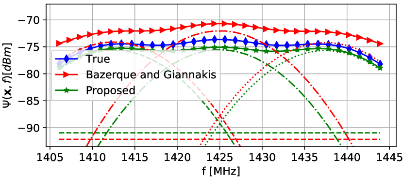
Figure 16: PSD reconstruction at a random location $\bm{x}\in\mathcal{X}$ where the basis expansion model uses Gaussian functions. The non-continuous red (green) curves represent the products ${{\color[rgb]{0,0,0}\hat{\pi}}}_{{\color[rgb]{0,0,0}b}}(\bm{x}){{\color[rgb]{0,0,0}\beta}}_{{{\color[rgb]{0,0,0}b}}}(f)$ estimated by the competing (proposed) algorithm.

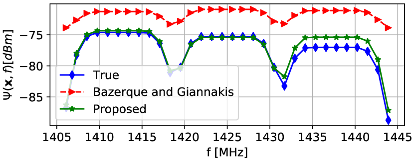
Figure 17: PSD reconstruction at $\bm{x}\in\mathcal{X}$ with a signal basis formed by using raised-cosine functions.

IV-D PSD Cartography

This section provides empirical support for the approach proposed in Sec. III-C2 for PSD cartography. To this end, each sensor samples the received PSD at $N_{f}=32$ uniformly spaced frequency values in the band of interest. The performance of the proposed method is compared with that of the non-negative Lasso algorithm in [3] with regularization parameter $10^{-11}$, which yields approximately the best RMSE. To improve its performance, this algorithm was extended to assume that the noise power is the same at all sensors.

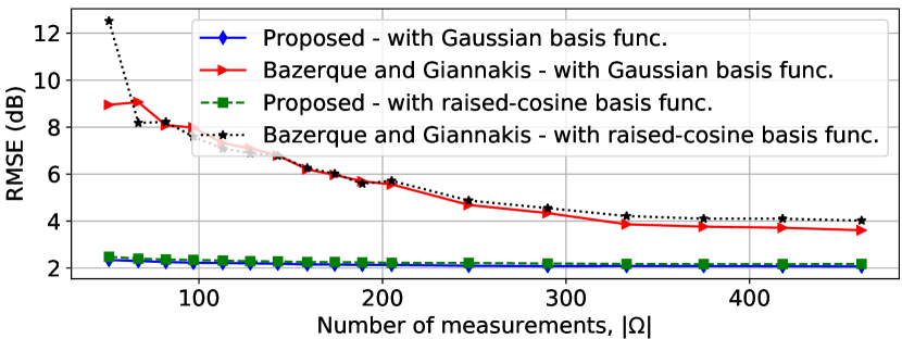
Figure 18: Performance comparison of the proposed scheme with that of the algorithm in [3].

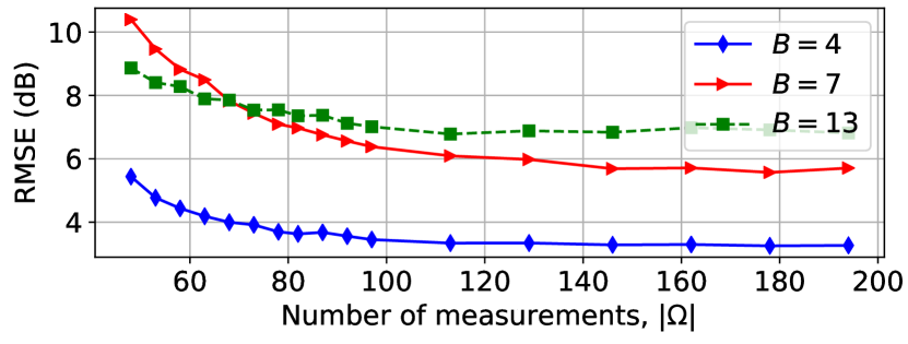
Figure 19: Map estimate RMSE of the proposed scheme for PSD cartography. The training and testing maps were obtained from the Wireless InSite data set, $Q_{t}=5$.

IV-D1 Gudmundson Data Set

The first part of this section evaluates the approaches in Sec. III-C and assesses the performance of the proposed algorithms using the training strategies in Sec. III-E1 when the training and testing maps were obtained from the Gudmundson data set. The $B-1=3$ signal basis functions are uniformly spaced across the band, whereas a fourth constant basis function is introduced to model noise; see Sec. III-C2. Two types of signal basis functions are investigated: Gaussian radial basis functions with standard deviation 5 MHz and raised-cosine functions with roll-off factor 0.4 and bandwidth 10 MHz. The noise basis function is scaled to yield $\upsilon(\bm{x},f)=\upsilon$, where $\upsilon$ is a uniform random variable between $-100$ and $-90$ dBm/MHz.

Fig. 14 demonstrates the superiority of the completion autoencoder when the output layers proposed in Sec. III-C2 are utilized relative to the weight-sharing scheme from Sec. III-C1. The reason is that the latter does not exploit prior information in the frequency domain. This output layer will be used in all remaining experiments.

The top row of Fig. 15 portrays the maps of the true coefficients $\{{{\color[rgb]{0,0,0}\pi}}_{{\color[rgb]{0,0,0}b}}(\bm{x})\}_{{{\color[rgb]{0,0,0}b}}=1}^{4}$ over $\mathcal{X}$; the second and last rows show their estimates with both schemes when $|\Omega|=512$. Visually, the proposed scheme produces better estimates despite the fact that it does not exploit the fact that the noise power is the same at all sensors. To demonstrate the reconstruction quality of the proposed scheme, Figs. 16 and 17 show the true and estimated PSDs at a random location $\bm{x}\in\mathcal{X}$. As observed, the PSD estimate produced by the proposed scheme follows the true PSD more closely compared to the one produced by the competing algorithm. A quantitative comparison is provided in Fig. 18, which shows the RMSE as a function of the number of measurements $|\Omega|$. As observed, the proposed method outperforms the competing approach with significant margin for small $|\Omega|$.

IV-D2 Wireless Insite Data Set

The second part of this section evaluates the performance of the proposed scheme using the training approach in Sec. III-E2, where the sets $\Omega_{t,q}^{(I)}$ and $\Omega_{t,q}^{(O)}$ are drawn from $\Omega_{t}$ uniformly at random without replacement with $|\Omega_{t,q}^{(I)}|=|\Omega_{t,q}^{(O)}|=1/2|\Omega_{t}|$, $q=1,\ldots,Q_{t}$, and $Q_{t}=5~{}\forall t$. The training and testing maps were obtained from the Wireless InSite data set. The transmit PSD is generated with the raised-cosine functions described in Sec. IV-D1. The noise PSD is set to $\upsilon(\bm{x},f)=\upsilon$, where $\upsilon$ is a uniform random variable between $-180$ and $-170$ dBm/MHz. Fig. 19 shows the RMSE of the proposed method as a function of the number of measurements $|\Omega|$. Because of the high RMSE of the competing approach [3] (possibly in part due to the reasons in Remark 4), its performance is not shown on the figure. As observed, the proposed scheme yields a low RMSE in this realistic scenario which emulates training with real measurements.

To conclude, it is worth stressing the computational efficiency of the trained autoencoder when estimating radio maps, since a simple forward pass is required. This contrasts with state-of-the-art alternatives, which generally require the application of iterative algorithms or the inversion of large matrices. As a reference, using our implementations for power map estimation in Fig. 8a on an Intel Core i7-6820HQ CPU, the proposed scheme takes $25\cdot 10^{-3}$ seconds, whereas the kriging, multi-kernel, GPR, and KNN methods respectively need $10^{-1}$, $1.25$, $3\cdot 10^{-1}$, and $4\cdot 10^{-1}$ seconds. For PSD map estimation, the run-time of the proposed algorithm is around $2.12\cdot 10^{-1}$ seconds whereas that of the algorithm in [3] is $6.43$ seconds.

V Conclusions and Discussion

Data-driven radio map estimation has been proposed to learn the spatial structure of propagation phenomena such as shadowing, reflection, and diffraction. Provided that sufficiently realistic data sets are available, learning such structure from past measurements yields estimators that require fewer measurements than state-of-the-art alternatives to attain a target performance. Motivated by the observation that radio maps lie close to a low-dimensional manifold embedded in a high-dimensional space, a deep completion network with an encoder-decoder architecture was proposed to estimate PSD maps. Extensive numerical experiments with two datasets reveal that the resulting scheme can attain an RMSE in the order of 2 dB, significantly better than existing approaches. The price to be paid for such an improved performance is the need for a training data set and increased computational demands compared to traditional “interpolation” approaches. Besides, deep neural networks typically require large data sets and obtaining the latter may be costly when one relies on measurements or ray tracing algorithms. However, this is a common limitation of any reasonable data-driven approach and can be alleviated by means of transfer learning. Future work will include mapping other channel metrics such as channel-gain with alternative network architectures.

References

- [1] Y. Teganya and D. Romero, “Data-driven spectrum cartography via deep completion autoencoders,” in Proc. IEEE Int. Conf. Commun., Dublin, Ireland, Jul. 2020, pp. 1–7.
- [2] A. Alaya-Feki, S. B. Jemaa, B. Sayrac, P. Houze, and E. Moulines, “Informed spectrum usage in cognitive radio networks: Interference cartography,” in Proc. IEEE Int. Symp. Personal, Indoor Mobile Radio Commun., Cannes, France, Sep. 2008, pp. 1–5.
- [3] J.-A. Bazerque and G. B. Giannakis, “Distributed spectrum sensing for cognitive radio networks by exploiting sparsity,” IEEE Trans. Signal Process., vol. 58, no. 3, pp. 1847–1862, Mar. 2010.
- [4] B. A. Jayawickrama, E. Dutkiewicz, I. Oppermann, G. Fang, and J. Ding, “Improved performance of spectrum cartography based on compressive sensing in cognitive radio networks,” in Proc. IEEE Int. Commun. Conf., Budapest, Hungary, Jun. 2013, pp. 5657–5661.
- [5] H. B. Yilmaz, T. Tugcu, F. Alagöz, and S. Bayhan, “Radio environment map as enabler for practical cognitive radio networks,” IEEE Commun. Mag., vol. 51, no. 12, pp. 162–169, Dec. 2013.
- [6] P. Huang, O. Castañeda, E. Gönültaş, S. Medjkouh, O. Tirkkonen, T. Goldstein, and C. Studer, “Improving channel charting with representation-constrained autoencoders,” in Proc. IEEE Int. Workshop Signal Process. Advances Wireless Commun., Cannes, France, Jul. 2019, pp. 1–5.
- [7] N. Patwari and P. Agrawal, “Effects of correlated shadowing: Connectivity, localization, and RF tomography,” in Int. Conf. Info. Process. Sensor Networks, St. Louis, MO, Apr. 2008, pp. 82–93.
- [8] D. Romero, Donghoon Lee, and G. B. Giannakis, “Blind radio tomography,” IEEE Trans. Signal Process., vol. 66, no. 8, pp. 2055–2069, 2018.
- [9] S. Grimoud, S. B. Jemaa, B. Sayrac, and E. Moulines, “A REM enabled soft frequency reuse scheme,” in Proc. IEEE Global Commun. Conf., Miami, FL, Dec. 2010, pp. 819–823.
- [10] E. Dall’Anese, S.-J. Kim, G. B. Giannakis, and S. Pupolin, “Power control for cognitive radio networks under channel uncertainty,” IEEE Trans. Wireless Commun., vol. 10, no. 10, pp. 3541–3551, Aug. 2011.
- [11] D. Romero, S-J. Kim, G. B. Giannakis, and R. López-Valcarce, “Learning power spectrum maps from quantized power measurements,” IEEE Trans. Signal Process., vol. 65, no. 10, pp. 2547–2560, May 2017.
- [12] S. Zhang and R. Zhang, “Radio map based 3d path planning for cellular-connected UAV,” in Proc. IEEE Global Commun. Conf., Waikoloa, HI, Dec. 2019, pp. 1–6.
- [13] D. Romero and G. Leus, “Non-cooperative aerial base station placement via stochastic optimization,” in Proc. IEEE Mobile Ad-hoc Sensor Netw., Shenzhen, China, Dec. 2019, pp. 131–136.
- [14] E. Bulut and I. Guevenc, “Trajectory optimization for cellular-connected uavs with disconnectivity constraint,” in Proc. IEEE Int. Conf. Commun., Kansas City, MO, May 2018, pp. 1–6.
- [15] J. Chen and D. Gesbert, “Optimal positioning of flying relays for wireless networks: A LOS map approach,” in Proc. IEEE Int. Conf. Commun., Paris, France, May 2017, pp. 1–6.
- [16] A. Goldsmith, Wireless Communications, Cambridge University Press, 2005.
- [17] R. Wahl, G. Wölfle, P. Wertz, P. Wildbolz, and F. Landstorfer, “Dominant path prediction model for urban scenarios,” Dresden, Germany, Jun. 2005, pp. 1–5.
- [18] K. R. Schaubach, N. J. Davis, and T. S. Rappaport, “A ray tracing method for predicting path loss and delay spread in microcellular environments,” in Proc. IEEE Veh. Technol. Conf., Denver, CO, USA, May 1992, pp. 932–935.
- [19] C. Parera, Q. Liao, I. Malanchini, C. Tatino, A. E. C. Redondi, and M. Cesana, “Transfer learning for tilt-dependent radio map prediction,” IEEE Trans. Cognitive Commun. Networking, vol. 6, no. 2, pp. 829–843, Jan. 2020.
- [20] T. Imai, K. Kitao, and M. Inomata, “Radio propagation prediction model using convolutional neural networks by deep learning,” in Proc. IEEE European Conf. Antennas Propag., Krakow, Poland, Apr. 2019, pp. 1–5.
- [21] K. Saito, Y. Jin, C. Kang, J.-I. Takada, and J.-S. Leu, “Two-step path loss prediction by artificial neural network for wireless service area planning,” IEICE Commun. Express, vol. 1–6, Sep. 2019.
- [22] T. Hayashi, T. Nagao, and S. Ito, “A study on the variety and size of input data for radio propagation prediction using a deep neural network,” in Proc. IEEE European Conf. Antennas Propag., Copenhagen, Denmark, Jul. 2020, pp. 1–5.
- [23] M. Iwasaki, T. Nishio, M. Morikura, and K. Yamamoto, “Transfer learning-based received power prediction with ray-tracing simulation and small amount of measurement data,” arXiv preprint arXiv:2005.00833, 2020.
- [24] R. Levie, Ç. Yapar, G. Kutyniok, and G. Caire, “Radiounet: Fast radio map estimation with convolutional neural networks,” arXiv preprint arXiv:1911.09002, 2019.
- [25] R. Levie, Ç. Yapar, G. Kutyniok, and G. Caire, “Pathloss prediction using deep learning with applications to cellular optimization and efficient d2d link scheduling,” in Proc. IEEE Int. Conf. Acoust., Speech, Signal Process., Barcelona, Spain, May 2020, pp. 8678–8682.
- [26] A. Agarwal and R. Gangopadhyay, “Predictive spectrum occupancy probability-based spatio-temporal dynamic channel allocation map for future cognitive wireless networks,” Trans. Emerging Telecommun. Technol., vol. 29, no. 8, pp. e3442, 2018.
- [27] G. Boccolini, G. Hernandez-Penaloza, and B. Beferull-Lozano, “Wireless sensor network for spectrum cartography based on kriging interpolation,” in Proc. IEEE Int. Symp. Personal, Indoor Mobile Radio Commun., Sydney, NSW, Nov. 2012, pp. 1565–1570.
- [28] D. Romero, R. Shrestha, Y. Teganya, and S. P. Chepuri, “Aerial spectrum surveying: Radio map estimation with autonomous UAVs,” in Proc. IEEE Int. Workshop Mach. Learn. Signal Process., Espoo, Finland, Sep. 2020, pp. 1–6.
- [29] S.-J. Kim, N. Jain, G. B. Giannakis, and P. Forero, “Joint link learning and cognitive radio sensing,” in Proc. Asilomar Conf. Signal, Syst., Comput., Pacific Grove, CA, Nov. 2011, pp. 1415 –1419.
- [30] S.-J. Kim and G. B. Giannakis, “Cognitive radio spectrum prediction using dictionary learning,” in Proc. IEEE Global Commun. Conf., Atlanta, GA, Dec. 2013, pp. 3206 – 3211.
- [31] G. Ding, J. Wang, Q. Wu, Y.-D. Yao, F. Song, and T. A Tsiftsis, “Cellular-base-station-assisted device-to-device communications in TV white space,” IEEE J. Sel. Areas Commun., vol. 34, no. 1, pp. 107–121, Jul. 2016.
- [32] D.-H. Huang, S.-H. Wu, W.-R. Wu, and P.-H. Wang, “Cooperative radio source positioning and power map reconstruction: A sparse Bayesian learning approach,” IEEE Trans. Veh. Technol., vol. 64, no. 6, pp. 2318–2332, Aug. 2014.
- [33] M. Hamid and B. Beferull-Lozano, “Non-parametric spectrum cartography using adaptive radial basis functions,” in Proc. IEEE Int. Conf. Acoust., Speech, Signal Process., New Orleans, LA, Mar. 2017, pp. 3599–3603.
- [34] S. Zha, J. Huang, Y. Qin, and Z. Zhang, “An novel non-parametric algorithm for spectrum map construction,” in Proc. IEEE Int. Symp. Electromagn. Compat., Amsterdam, Netherlands, Aug. 2018, pp. 941–944.
- [35] Y. Teganya, D. Romero, L. M. Lopez-Ramos, and B. Beferull-Lozano, “Location-free spectrum cartography,” IEEE Trans. Signal Process., vol. 67, no. 15, pp. 4013–4026, Aug. 2019.
- [36] J.-A. Bazerque, G. Mateos, and G. B. Giannakis, “Group-lasso on splines for spectrum cartography,” IEEE Trans. Signal Process., vol. 59, no. 10, pp. 4648–4663, Oct. 2011.
- [37] J.-A. Bazerque and G. B. Giannakis, “Nonparametric basis pursuit via kernel-based learning,” IEEE Signal Process. Mag., vol. 28, no. 30, pp. 112–125, Jul. 2013.
- [38] M. Tang, G. Ding, Q. Wu, Z. Xue, and T. A. Tsiftsis, “A joint tensor completion and prediction scheme for multi-dimensional spectrum map construction,” IEEE Access, vol. 4, pp. 8044–8052, Nov. 2016.
- [39] G. Zhang, X. Fu, J. Wang, and M. Hong, “Coupled block-term tensor decomposition based blind spectrum cartography,” in Proc. Asilomar Conf. Signal, Syst., Comput., Pacific Grove, CA, Nov. 2019, pp. 1644–1648.
- [40] S.-J. Kim, E. Dall’Anese, and G. B. Giannakis, “Cooperative spectrum sensing for cognitive radios using Kriged Kalman filtering,” IEEE J. Sel. Topics Signal Process., vol. 5, no. 1, pp. 24–36, Jun. 2010.
- [41] D. Lee, S.-J. Kim, and G. B. Giannakis, “Channel gain cartography for cognitive radios leveraging low rank and sparsity,” IEEE Trans. Wireless Commun., vol. 16, no. 9, pp. 5953–5966, Jun. 2017.
- [42] D. Lee, D. Berberidis, and G. B. Giannakis, “Adaptive bayesian radio tomography,” IEEE Trans. Signal Process., vol. 67, no. 8, pp. 1964–1977, Mar. 2019.
- [43] X. Han, L. Xue, F. Shao, and Y. Xu, “A power spectrum maps estimation algorithm based on generative adversarial networks for underlay cognitive radio networks,” Sensors, vol. 20, no. 1, pp. 311, Jan. 2020.
- [44] A. Felix, S. Cammerer, S. Dörner, J. Hoydis, and S. Ten Brink, “OFDM-autoencoder for end-to-end learning of communications systems,” in Proc. IEEE Int. Workshop Signal Process. Advances Wireless Commun., Kalamata, Greece, Jun. 2018, pp. 1–5.
- [45] P. Stoica and R. L. Moses, Spectral analysis of signals, Upper Saddle River, NJ, USA: Prentice-Hall, 2005.
- [46] I. Goodfellow, Y. Bengio, and A. Courville, Deep learning, Cambridge, MA, USA: MIT press, 2016.
- [47] B. R. Hamilton, X. Ma, R. J. Baxley, and S. M. Matechik, “Propagation modeling for radio frequency tomography in wireless networks,” IEEE J. Sel. Topics Signal Process., vol. 8, no. 1, pp. 55–65, Feb. 2014.
- [48] J. Fan and T. Chow, “Deep learning based matrix completion,” Neurocomputing, vol. 266, pp. 540–549, Nov. 2017.
- [49] V. Cherkassky and F. M. Mulier, Learning from Data: Concepts, Theory, and Methods, John Wiley & Sons, 2007.
- [50] S. Iizuka, E. Simo-Serra, and H. Ishikawa, “Globally and locally consistent image completion,” ACM Trans. Graphics, vol. 36, no. 4, pp. 107, Jul. 2017.
- [51] G. Vázquez-Vilar and R. López-Valcarce, “Spectrum sensing exploiting guard bands and weak channels,” IEEE Trans. Signal Process., vol. 59, no. 12, pp. 6045–6057, Sep. 2011.
- [52] D. Romero and G. Leus, “Wideband spectrum sensing from compressed measurements using spectral prior information,” IEEE Trans. Signal Process., vol. 61, no. 24, pp. 6232–6246, Dec. 2013.
- [53] R. Tandra and A. Sahai, “SNR walls for signal detection,” IEEE J. Sel. Topics Signal Process., vol. 2, no. 1, pp. 4–17, Feb. 2008.
- [54] M. Ribeiro, A. E. Lazzaretti, and H. S. Lopes, “A study of deep convolutional auto-encoders for anomaly detection in videos,” Pattern Recognition Letters, vol. 105, pp. 13–22, Apr. 2018.
- [55] K. He, X. Zhang, S. Ren, and J. Sun, “Delving deep into rectifiers: Surpassing human-level performance on imagenet classification,” in Proc. IEEE Int. Conf. Comput. Vision, Washington, DC, Dec. 2015, pp. 1026–1034.
- [56] V. Dumoulin and F. Visin, “A guide to convolution arithmetic for deep learning,” arXiv preprint arXiv:1603.07285, 2016.
- [57] M. C Jeruchim, P. Balaban, and K. S. Shanmugan, Simulation of communication systems: modeling, methodology and techniques, New York, NY, USA: Academic, 2006.
- [58] M. Gudmundson, “Correlation model for shadow fading in mobile radio systems,” Electron. Letters, vol. 27, no. 23, pp. 2145–2146, Nov. 1991.
- [59] H. Ling, R.-C. Chou, and S.-W. Lee, “Shooting and bouncing rays: Calculating the rcs of an arbitrarily shaped cavity,” IEEE Trans. Antennas Propag., vol. 37, no. 2, pp. 194–205, Feb. 1989.
- [60] F. Pérez Fontán and P. Mariño Espiñeira, Modeling the wireless propagation channel: a simulation approach with Matlab, Wiley, 2008.
- [61] D. P. Kingma and J. L. Ba, “Adam: A method for stochastic optimization,” arXiv preprint arXiv:1412.6980, 2014.
- [62] C. E. Rasmussen and C. K. I. Williams, Gaussian Processes for Machine Learning, vol. 2, Cambridge, MA, USA: MIT Press, 2006.