Predictive Dirac and Majorana Neutrino Mass Textures from Grand Unified Theories
Abstract
We present simple and predictive realizations of neutrino masses in theories based on the grand unifying group. At the level of the lowest-dimension operators, this class of models predicts a skew-symmetric flavor structure for the Dirac mass term of the neutrinos. In the case that neutrinos are Dirac particles, the lowest-order prediction of this construction is then one massless neutrino and two degenerate massive neutrinos. Higher-dimensional operators suppressed by the Planck scale perturb this spectrum, allowing a good fit to the observed neutrino mass matrix. A firm prediction of this construction is an inverted neutrino mass spectrum with the lightest neutrino hierarchically lighter than the other two, so that the sum of neutrino masses lies close to the lower bound for an inverted hierarchy. In the alternate case that neutrinos are Majorana particles, the mass spectrum can be either normal or inverted. However, the lightest neutrino is once again hierarchically lighter than the other two, so that the sum of neutrino masses is predicted to lie close to the corresponding lower bound for the normal or inverted hierarchy. Near future cosmological measurements will be able to test the predictions of this scenario for the sum of neutrino masses. In the case of Majorana neutrinos that exhibit an inverted hierarchy, future neutrinoless double beta experiments can provide a complementary probe.
I Introduction
Multiple neutrino oscillation experiments over the past two decades have conclusively established that neutrinos have non-vanishing masses Tanabashi:2018oca , thereby providing concrete evidence of new physics beyond the Standard Model (SM). However, although these experiments have measured the neutrino mass splittings and mixing angles, the actual values of the neutrino masses still remain unknown. In particular, it is not known whether the neutrino mass spectrum exhibits a normal or inverted hierarchy. Several medium and long-baseline neutrino oscillation experiments have been proposed to settle this issue Qian:2015waa . At present, the important question of whether neutrinos are Dirac or Majorana fermions also remains unanswered. Future neutrinoless double beta decay () experiments may be able to resolve this question Dolinski:2019nrj .
Grand unification Pati:1974yy ; Georgi:1974sy ; Langacker:1980js is one of the most attractive proposals for physics beyond the SM. In these theories, the strong, weak and electromagnetic interactions of the SM are unified into a larger grand unifying group. The fermions of the SM are embedded into representations of this bigger group, with the result that quarks and leptons are also unified into the same multiplets. These representations often contain additional SM singlets, which can naturally serve the role of right-handed neutrinos in the generation of neutrino masses. The fact that the SM quarks and leptons are now embedded together in the same multiplets often leads to relations between the masses of the different SM fermions Buras:1977yy . If these multiplets also contain right-handed neutrinos, these theories can impose restrictions on the form of the neutrino mass matrix, leading to predictions for the neutrino masses. Familiar examples of unified theories that can relate the masses of the neutrinos to those of the charged fermion include the Pati-Salam Pati:1974yy and Georgi:1974my ; Fritzsch:1974nn gauge groups.
In this paper we explore a class of models based on the grand unified theory (GUT) Kim:1981jw ; Fukugita:1981gn that lead to sharp predictions for the neutrino mass spectrum. In these theories, the right-handed neutrino emerges from the same multiplet as the lepton doublet of the SM. A natural consequence of this construction is that, at the level of the lowest-dimension terms, the Dirac mass term for the neutrinos is skew-symmetric in flavor space, so that the determinant of the Dirac mass matrix vanishes. If neutrinos are Dirac particles that obtain their masses from this term, then, in the absence of corrections to this form from terms of higher dimension, the neutrino mass spectrum consists of two degenerate species and a massless one. Once higher-dimensional terms suppressed by the Planck scale are included, this class of models can easily reproduce the observed spectrum of neutrino masses and mixings. A firm prediction of this construction is that the spectrum of neutrino masses is inverted, with the lightest neutrino hierarchically lighter than the other two. Then the sum of neutrino masses is predicted to lie close to the lower bound of 0.10 eV set by the observed mass splittings in the case of an inverted hierarchy. Future precision cosmological experiments, such as LSST Abell:2009aa , Euclid Amendola:2016saw , DESI Aghamousa:2016zmz , the Simons Observatory Ade:2018sbj , and CMB-S4 Abazajian:2019eic , that have the required sensitivity to the sum of neutrino masses will be able to test this striking prediction. The final phase of Project-8 Esfahani:2017dmu , with an expected sensitivity of 0.04 eV to the absolute electron neutrino mass, will also be able to test this scenario. Similarly, future large-scale long-baseline neutrino oscillation experiments, such as Hyper-K Abe:2018uyc and DUNE Abi:2018dnh , will be able to test the prediction regarding the inverted nature of the mass spectrum.
It is well-established that there is a lower bound on the light neutrino contribution to the process in the case of Majorana neutrinos that exhibit an inverted mass-hierarchy Vissani:1999tu ; Bilenky:2001rz . In particular, it has been pointed out that if long-baseline neutrino experiments determine that the neutrino mass hierarchy is inverted, while no signal is observed in down to the effective Majorana neutrino mass eV, then this would constitute compelling evidence that neutrinos are Dirac rather than Majorana fermions Mohapatra:2005wg . The model we present here is an example of a GUT framework that can naturally accommodate such a scenario.
If, in addition to the skew-symmetric Dirac mass term, there is also a large Majorana mass term for the right-handed neutrinos, the neutrinos will be Majorana particles. In this scenario, the skew-symmetric nature of the Dirac mass term implies that the lightest neutrino is massless, up to small corrections from higher-dimensional operators. In contrast to the case of Dirac neutrinos discussed above, the spectrum of neutrino masses can now exhibit either a normal or inverted hierarchy. However, the lightest neutrino is still predicted to be hierarchically lighter than the other two, so that for both normal and inverted hierarchies the sum of neutrino masses is predicted to lie close to the corresponding lower bound dictated by the observed mass splittings, i.e. 0.06 eV for the normal case and 0.10 eV for the inverted. This is a prediction that can be tested by future cosmological observations once long-baseline experiments have determined whether the spectrum is normal or inverted. In addition, these predictions for the sum of neutrino masses translate into upper and lower bounds on the rate for each of the normal and inverted cases, with important implications for future experiments. In our analysis, we explore both the Dirac and Majorana possibilities in detail and obtain realistic fits to the observed masses and mixings.
To understand the origin of the prediction that the Dirac mass term for the neutrinos is skew-symmetric, we first consider the minimal grand unifying symmetry, namely Georgi:1974sy . In this class of theories the grand unifying symmetry is broken at the unification scale, GeV, down to the SM gauge groups. In simple models based on , all the SM fermions in a single generation arise from the and representations. The is the anti-fundamental representation while the is the tensor representation with two antisymmetric indices. The Higgs field of the SM is contained in the fundamental representation, the . The up-type quark masses arise from Yukawa couplings of the schematic form , where contains the SM Higgs, is the 5-dimensional antisymmetric Levi-Civita tensor, and the Greek letters represent indices. Similarly, the down-type quark and charged lepton masses arise from Yukawa couplings of the form . Although attractive and elegant, the minimal model does not contain SM singlets that can play the role of right-handed neutrinos, and does not make predictions regarding the neutrino masses. Simple extensions of minimal to , however, do contain natural candidates for the role of right-handed neutrinos and also allow for elegant solutions to the doublet-triplet splitting problem Sen:1984aq ; Barr:1997pt ; Berezhiani:1989bd ; Barbieri:1993wz ; Dvali:1993yf ; Chacko:1998zz .
In the simplest extension of to , the SM fermions emerge from the and representations. While the is the antifundamental representation of , the is the tensor representation with two antisymmetric indices. Under the subgroup of , these representations decompose as and , and can be seen to contain particles with the quantum numbers of the SM fermions. But now, in addition, the singlet of contained in the representation is a natural candidate to play the role of the right-handed neutrino. If the SM Higgs emerges from the fundamental representation of , the down-type quarks and charged leptons can obtain masses from terms of the schematic form . However, with this set of representations it is not possible to obtain masses for the up-type quarks of the SM at the renormalizable level. This presents a problem because the top Yukawa coupling is large.
One possible solution to this problem, first explored in Refs. Barbieri:1994kw ; Berezhiani:1995dt , is that the third-generation up-type quarks emerge in part from the of , which is the tensor representation with three antisymmetric indices. This decomposes as under . This allows the third-generation up-type quarks to obtain their masses from a renormalizable term of the form . Nonrenormalizable operators suffice to generate masses for the up-type quarks of the lighter two generations.
The problem of the top quark mass in GUTs admits an alternative solution if electroweak symmetry is broken by two light Higgs doublets rather than one, so that the low-energy theory is a two-Higgs-doublet model. In this framework, one of Higgs doublets, which gives mass to the up-type quarks, is assumed to arise from the of . This allows all the up-type quark masses to be generated from renormalizable terms of the form , where the Higgs doublet is now contained in the Kim:1981jw . The other Higgs doublet, which arises from the of , gives mass to the down-type quarks and charged leptons. The central observation is that the same Higgs doublet in the that generates the large top quark mass can also be used to generate a Dirac neutrino mass term through renormalizable operators of the form , where and are flavor indices. Since the of is antisymmetric in its tensor indices, this vanishes if the flavor indices and are the same. Therefore, this construction naturally leads to a skew-symmetric structure for the Dirac mass matrix of the neutrinos in flavor space.
This framework can naturally accommodate either Dirac or Majorana neutrino masses. The right-handed neutrinos can naturally acquire large Majorana masses of order GeV from nonrenormalizable Planck-suppressed interactions with the Higgs fields that break the GUT symmetry. This naturally leads to Majorana masses for the neutrinos of the right size through the seesaw mechanism Minkowski:1977sc ; Mohapatra:1979ia ; Yanagida:1979as ; GellMann:1980vs . Alternatively, as a consequence of additional discrete symmetries, a Majorana mass term for the right-handed neutrinos may not be allowed, while the coefficient of the Dirac mass term is suppressed. In such a scenario we obtain Dirac neutrino masses. In this paper we will consider both the Dirac and Majorana cases.
This paper is organized as follows. In Section II, we outline the framework that underlies this class of models and show how the pattern of neutrino masses emerges in the Dirac and Majorana cases. In Section III, we present a realistic model in which the neutrino masses are Dirac, and perform a detailed numerical fit to the neutrino masses and mixings using a recent global analysis of the 3-neutrino oscillation data. We show that this framework predicts an inverted spectrum of neutrino masses with one mass eigenstate hierarchically lighter than the others. In Section IV, we present a realistic model in which the neutrino masses are Majorana, and again perform a detailed numerical fit to the neutrino oscillation data. We show that in this scenario one neutrino is again hierarchically lighter than the others, but the spectrum of neutrino masses can now be either normal or inverted. We also explore the implications of this scenario for future experiments and future cosmological observations. Our conclusions are presented in Section V.
II The Framework
Our model is based on the GUT symmetry with the fermions of each family arising from a representation, denoted by , and a rank-two antisymmetric representation , denoted by . For now we omit the generation indices. Note that anomaly cancellation for the group requires that there be two chiral fermion representations for each 15 fermion. We denote the additional of each family by . After the breaking of to , the fields in that carry charges under the SM gauge groups acquire large masses at the GUT scale by marrying the non-SM fermions in the . Therefore, these fields do not play a role in generating the masses of the light fermions. However, the SM-singlet field in , which has no counterpart in the , may remain light. We employ the familiar convention in which all fermions are taken to be left-handed, and the SM fermions are labelled as , with and .
The symmetry is broken near the GUT scale down to , which contains the usual embedding of SM fermions in a and a 10 of . Without loss of generality we take the indices to be , so that the index lies outside . Color indices run over .
We now consider the assignment of fermions under representations of . Under the fermion multiplet that transforms as a , we have
| (4) |
where is the SM lepton doublet, . Note that the Dirac partner of the SM neutrino is embedded in the same multiplet as the left-handed leptons. The fermions in also transform as :
| (8) |
The fermion content of , which transforms as a 15-dimensional representation of , is given by
| (15) |
The breaking of down to at the GUT scale is realized by a Higgs field which transforms as a under and acquires a large vacuum expectation value (VEV) along the SM-singlet direction. A Higgs field , which transforms as an adjoint under , further breaks down to the SM gauge group. The breaking of electroweak symmetry is realized through two Higgs doublets and that arise from different representations. The field , which gives masses to the down-type quarks and charged leptons, emerges from a 6 while , which gives masses to the up-type quarks, arises from a 15. The Higgs fields , and are assumed to have the following VEVs:
| (34) |
The VEV of takes the pattern
| (41) |
The field content is summarized in Table 1. Here denotes the number of flavors.
| Multiplets | representation | ||
| 3 | |||
| fermion | 3 | ||
| 15 | 3 | ||
| 1 | |||
| scalar | 1 | ||
| 1 | |||
| 35 | 1 | ||
We now discuss the generation of fermion masses. The additional fermions , in and , in acquire masses at the GUT scale through interactions with of the form
| (42) |
where we have suppressed the and Lorentz indices and shown only the flavor indices. Consequently, these fields do not play any role in the generation of the masses of the SM fermions. These interactions do not give mass to the SM-singlet field in . However, even if is light, the fact that it is a SM singlet means that in the absence of other interactions its couplings to the SM fields at low energies are very small.
The SM fermions acquire masses from their Yukawa couplings to the Higgs fields and after electroweak symmetry breaking. The -invariant Yukawa couplings take the form
| (43) |
The down-quark and charged-lepton masses arise from the term in the Lagrangian after the Higgs field acquires an electroweak-scale VEV. Similarly the up-quark masses arise from the term in the Lagrangian after acquires a VEV. In general, the masses of the SM fermions also receive contributions from higher-dimensional operators suppressed by the Planck scale () that involve , such as
| (44) |
The VEV of breaks the symmetry that relates quarks and leptons [cf. Eq. (41)]. Therefore these higher-dimensional operators violate the GUT symmetries that relate the masses of the down-type quarks to those of the leptons of the same generation.
A Dirac mass term for the neutrinos may be obtained from interactions of the form
| (45) |
As explained earlier, the fact that is an antisymmetric tensor under implies that is skew-symmetric in flavor space. Consequently, the resulting Dirac mass matrix for the neutrinos has vanishing determinant. We expect corrections to the Dirac mass term from Planck-suppressed higher-dimensional operators, such as
| (46) |
In general, this contribution will be suppressed by a factor relative to that from Eq. (45).
A large Majorana mass term for the right-handed neutrinos can be obtained from Planck-suppressed nonrenormalizable interactions of the form
| (47) |
This leads to Majorana masses for the right-handed neutrinos of order , which is parametrically of order the seesaw scale GeV. Then, from Eqs. (45) and (47), we obtain Majorana neutrino masses of the right size.
If neutrinos are to be Dirac particles, the mass term for the right-handed neutrinos shown in Eq. (47) must be absent. Furthermore, we require the coefficients of the Dirac mass terms to be extremely small, , to reproduce the observed values of the neutrino masses. In Section III, we shall show that the absence of the Majorana mass term for the right-handed neutrinos, Eq. (47), and the smallness of and can be explained on the basis of discrete symmetries.
III Dirac Neutrino Masses
III.1 Pattern of Neutrino Masses
We now present a simple model that realizes the pattern of Dirac neutrino masses discussed in Section II. The model is based on discrete symmetries under which the fermions and Higgs scalars have the charge assignments shown in Table 2.
| Multiplets | representation | quantum number | quantum number | |
|---|---|---|---|---|
| fermion | ||||
| scalar | ||||
| 35 | ||||
| 1 | ||||
The Yukawa couplings that generate masses for the SM fermions, Eqs. (43) and (44), are consistent with the and symmetries. The interaction in Eq. (42) that gives GUT-scale masses to the extra fermions , in and , in is also allowed by the discrete symmetries. However, the renormalizable Dirac mass term for the neutrinos, Eq. (45), is now forbidden by the discrete symmetry. Instead, the leading contribution to the neutrino masses arises from the dimension-5 term
| (48) |
The field , which is a singlet under , is assumed to acquire a VEV, thereby spontaneously breaking the discrete symmetry. For GeV, we obtain Dirac neutrino masses in the right range. Since is in an antisymmetric representation of , these mass terms are antisymmetric in flavor space, i.e.
| (49) |
This leads to a highly predictive spectrum, with one zero eigenvalue, and the other two eigenvalues equal in magnitude and opposite in sign. This corresponds to an inverted mass hierarchy, in which the smaller arises from the difference between the masses of the two heavier eigenstates. We can perform phase rotations on the right-handed neutrinos to ensure that the elements of this mass matrix are real, so that the phase in the PMNS matrix vanishes.
Clearly, the mass pattern above is ruled out experimentally. However, we need to include the effects of higher-dimensional terms, which will give corrections to the pattern above. Since these corrections are expected to be small, we expect to retain the qualitative features of the spectrum above, in particular, an inverted ordering. An example of such a higher-dimensional operator is the dimension-6 term
| (50) |
This correction is parametrically smaller than the antisymmetric contribution in Eq. (48) by a factor .
In order for the terms in Eq. (48) to give rise to the leading contribution to the neutrino masses, other possible mass terms involving the light neutrino fields and must be suppressed. The discrete symmetry forbids Majorana mass terms for and . It also forbids Dirac mass terms between and . A Dirac mass term between and can be generated as a -breaking effect, but only at dimension-8:
| (51) |
This is too small to have any observable effect. Therefore, without loss of generality, the neutrino mass matrix has the form of a real skew-symmetric matrix with a small complex symmetric component. We write the mass term in matrix form as,
| (56) |
It is convenient to decompose the Dirac mass matrix as,
| (57) |
Here is skew-symmetric and takes the form
| (61) |
while is an anarchic symmetric matrix whose entries are parametrically smaller than those in . We can choose and in Eq. (61) to be real without loss of generality. However, in general the elements of are complex.
The PMNS matrix is, as usual, defined to be the rotation matrix that relates the flavor eigenstates of the active neutrinos to the mass eigenstates :
| (68) |
Defining as the diagonalized mass matrix with mass eigenvalues corresponding to the eigenstates , we have
| (69) |
Therefore the PMNS matrix is identified with the matrix that diagonalizes the matrix . By a suitable choice of of , and the elements in , we can fit the observed neutrino mass splittings and mixing angles.
Before proceeding with a numerical scan, we first estimate the region of parameter space consistent with observations. Although there are a large number of free parameters, since only and are expected to be large, this scenario is very predictive. We parametrize the elements of the skew-symmetric matrix as follows:
| (70) |
Since arises from a higher-dimensional operator, it can be treated as a perturbation. At zeroth order in this perturbation, the eigenvalues for are simply . This corresponds to a limiting case of an inverted mass hierarchy in which the smaller (solar) mass splitting vanishes. By convention, in an inverted hierarchy the mass eigenstates are labeled such that corresponds to the mass of the lightest state and the smaller splitting is between and , with . In our case, these correspond to the masses of two degenerate eigenstates with mass . Then the eigenstate with vanishing mass is identified as . The mixing angle mixes states in the degenerate subspace, and hence is arbitrary at this order. It will be fixed by the perturbation. The other two mixing angles are given by and . The Dirac phase can be rotated away at this order as well.
To summarize, for , which corresponds to zeroth order in the perturbation, the model predictions for the solar and atmospheric mass-squared splittings, the mixing angles, and the Dirac phase are given by
| (71) |
where . Once we add the perturbation , the solar splitting and the mixing angle are fixed. The perturbation can be parametrized as , where is an anarchic symmetric matrix with entries of order . The lightest eigenstate acquires a mass of order from the perturbation, and the solar splitting is now
| (72) |
The atmospheric mass splitting continues to remain of the order of . The ratio of the solar and atmospheric splittings determines the parametric size of , which in turn sets the mass of the lightest eigenstate. Putting in the numbers, we have
| (73) |
We see that a satisfactory fit to the data requires the parameter to be of order . Remarkably, this is in excellent agreement with the expected value of from our construction, .
We see that this flavor pattern results in a very predictive spectrum of neutrino masses and mixings. We obtain an inverted mass hierarchy, with one neutrino hierarchically lighter than the other two. This prediction can be conclusively tested in future long-baseline oscillation experiments such as Hyper-K Abe:2018uyc and DUNE Abi:2018dnh . Since the -violating phase in the PMNS matrix vanishes in the limit that is zero, it might have been expected to be small. However, the results of our numerical scans in Section III.2 show that this need not be the case, and that fairly large values of can be obtained even for .
| Fit | ||||||||
|---|---|---|---|---|---|---|---|---|
| Fit 1 (IH) | 0.0620 | 0.0180 | 0.0410 | 0.0088 | 0.0184 | 0.0075 | - | |
| Fit 2 (IH) | 0.1012 | 0.0234 | 0.0202 | 0.0113 | 0.0151 | 0.0022 | - | |
| Fit 3 (IH) | 0.0620 | 0.0604 | 0.0239 | 0.0038 | 0.0236 | 0.0041 |
| Oscillation | allowed range | Model prediction | ||
| parameters | from NuFit4.1 Esteban:2018azc | Fit 1 (IH) | Fit 2 (IH) | Fit 3 (IH) |
| ) | 6.79 - 8.01 | 7.35 | 7.39 | 7.41 |
| 2.416 - 2.603 | 2.540 | 2.506 | 2.540 | |
| 0.275 - 0.350 | 0.319 | 0.314 | 0.305 | |
| 0.430 - 0.612 | 0.557 | 0.558 | 0.559 | |
| 0.02066 - 0.02461 | 0.0230 | 0.0224 | 0.0227 | |
| 205 - 354 | 330.8 | 277.7 | 287.7 | |
| () | - | |||
|
|
III.2 Fits to the Data
Our strategy for the scan is as follows. The neutrino mass matrix is parameterized in terms of a skew-symmetric matrix with a small symmetric correction , as discussed in Section III.1. We fix the parameters of the skew-symmetric matrix in Eq. (61) such that the zeroth order predictions match the measured values of , and as given by Eq. (71). In particular, we take eV2, , and corresponding to the central values from NuFit Esteban:2018azc for the inverted hierarchy case and employ Eq. (70) to determine , and . Further, the size of the perturbation is fixed by . We then scan over the anarchic matrix and obtain numerical predictions for the entire PMNS matrix. We choose to parametrize the mass matrix in Eq. (57) in terms of and the ratios , and ,
| (83) |
As can be seen from Eq. (70), the values of and are fixed at 4.393 and 4.931, respectively. The elements of the perturbation matrix are restricted to be much smaller than , , and . The input parameters shown in Table 4 are examples of fits that are in excellent agreement with the recent global fit results from NuFit Esteban:2018azc . In obtaining these fits, all the elements of have been taken to be real except and . We have introduced phases and in the elements and respectively in order to obtain a non-zero phase in the PMNS matrix. Although the addition of just a single phase, say , can give us a non-vanishing (as in Fits 1 and 2), we find that in this case a large requires a somewhat larger value of (as in Fit 2). The addition of a second phase allows us to obtain a large even if all the are small (as in Fit 3).
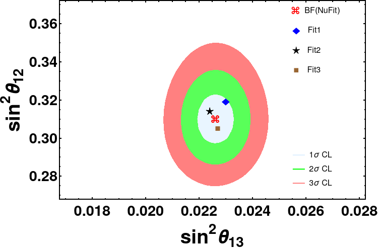
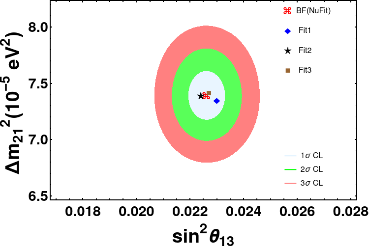
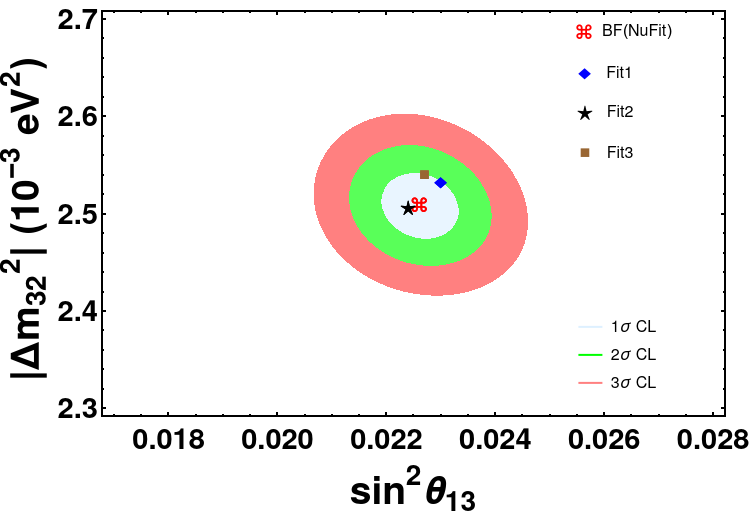
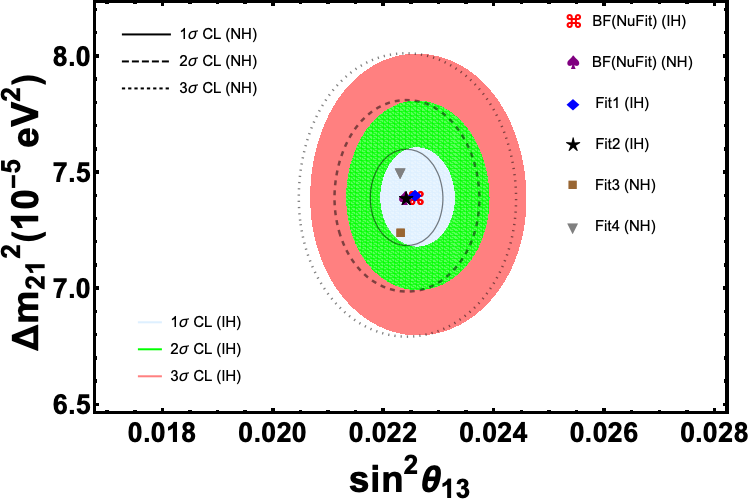
The predictions of these fits for the oscillation parameters are shown in Table 4, along with the allowed range from NuFit4.1 global analysis Esteban:2018azc . Also included are the predictions for the mass of the lightest neutrino. Note that in each of these fits the lightest neutrino mass is hierarchically lighter than the other two mass eigenstates by more than two orders of magnitude. The results for the fits presented in Table 4 are also displayed in Fig. 1 as Fit1, Fit2 and Fit3 in a two-dimensional projection of the (gray), (green), and (pink) confidence level (CL) regions of the global-fit results (without the inclusion of the Super-K atmospheric -data). The NuFit best-fit points in each plane are shown by the red markers, while the blue, black and brown markers correspond to Fit1, Fit2 and Fit3 respectively.
Interestingly, we find no significant restriction on the -violating phase in the PMNS matrix in this scenario. In particular, as seen from Fit 3, we can get a large phase in the PMNS matrix even if all the elements of are smaller by a factor of order than the observed atmospheric splitting. Larger values seem to be preferred by the recent T2K results Abe:2019vii , and in the future, a more precise determination of can only help us better constrain the parameter space of the model.
IV Majorana Neutrino Masses
IV.1 Pattern of Neutrino Masses
We now present a simple model in which the pattern of Majorana neutrino masses discussed in Section II is realized. The model is based on a discrete symmetry under which the fermions and Higgs scalars have the charge assignments shown in Table 5.
| Multiplets | representation | quantum number | |
|---|---|---|---|
| fermion | |||
| scalar | |||
| 35 | 0 | ||
With this choice of charge assignments the interaction in Eq. (42) that gives GUT-scale masses to the extra fermions , in and , in is allowed by the discrete symmetry. The Yukawa couplings that generate masses for the SM quarks and charged leptons, Eqs. (43) and (44), are also allowed. Turning our attention to the neutrino sector, the renormalizable Dirac mass term for the neutrinos, Eq. (45), and the nonrenormalizable Majorana mass term for the right-handed neutrinos, Eq. (47), are both consistent with the discrete symmetry. In the absence of other mass terms involving and , these interactions lead to the desired pattern of Majorana neutrino masses. The singlet neutrinos in obtain large Majorana masses of order the right-handed scale through the operator
| (84) |
The discrete symmetry forbids a renormalizable Dirac mass term between the SM neutrinos and the singlet neutrinos . Any allowed Dirac mass terms between and are highly Planck suppressed and much smaller than their Majorana masses. It follows that the effects of on the neutrino masses are small and can be neglected. Then, the Dirac mass term in Eq. (45) and the Majorana mass term in Eq. (47) give the dominant contributions to the neutrino masses, leading to Majorana neutrino masses of parametrically the right size that exhibit the pattern discussed in Section II.
| Fit | (eV) | ||||||||
|---|---|---|---|---|---|---|---|---|---|
| Fit 1 (IH) | 4.152 | 5.100 | 0.9937 | 0.8351 | 0.0537 | 0.0877 | |||
| Fit 2 (IH) | 4.459 | 4.868 | 0.9773 | 0.8608 | 0.0458 | 0.0745 | |||
| Fit 3 (NH) | 0.5116 | 0.4549 | 0.1330 | -0.7430 | 0.0990 | 0.0263 | |||
| Fit 4 (NH) | 0.4983 | 0.4614 | 0.1211 | -0.6934 | 0.0980 | 0.0425 |
| Oscillation | allowed range | Model prediction | |||
| parameters | from NuFit4.1 Esteban:2018azc | Fit 1 (IH) | Fit 2 (IH) | Fit 3 (NH) | Fit 4 (NH) |
| ) | 6.79 - 8.01 | 7.40 | 7.39 | 7.24 | 7.50 |
| (IH) | 2.416 - 2.603 | 2.509 | 2.504 | - | - |
| (NH) | 2.432 - 2.618 | - | - | 2.532 | 2.500 |
| 0.275 - 0.350 | 0.309 | 0.310 | 0.303 | 0.300 | |
| (IH) | 0.430 - 0.612 | 0.590 | 0.544 | - | - |
| (NH) | 0.427 - 0.609 | - | - | 0.516 | 0.527 |
| (IH) | 0.02066 - 0.02461 | 0.02258 | 0.02241 | - | - |
| (NH) | 0.02046 - 0.02440 | - | - | 0.02232 | 0.02231 |
| (IH) | 205 - 354 | 296.3 | 286.4 | - | - |
| (NH) | 141 - 370 | - | - | 282.3 | 277.2 |
|
|
IV.2 Fits to the data
In this subsection, we obtain fits to the neutrino masses and mixings for the case of Majorana neutrinos. The skew-symmetric Dirac mass matrix and symmetric Majorana mass matrix are parameterized as
| (85) |
In the limit that , we can write the following seesaw relation for the light neutrino masses,
| (86) |
where we choose to parametrize the mass matrix in terms of , , and . The overall mass scale is required to be tiny, of order GeV, to obtain the observed values of neutrino masses. We perform a numerical scan of the input parameters, as shown in Eq. (86), to obtain predictions for the entire PMNS matrix. It is beyond the scope of this work to scan over the full parameter space; instead, we perform a constrained minimization in which the five neutrino observables (, and with in the case of normal hierarchy and for inverted) are restricted to lie within of their experimentally measured values. The parameter has been chosen to be complex in order to induce a violating phase in the PMNS matrix, but the other parameters have been taken to be real. We emphasize that the lightest neutrino is exactly massless due to the skew-symmetric nature of the Dirac mass matrix .
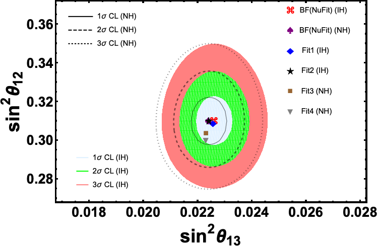
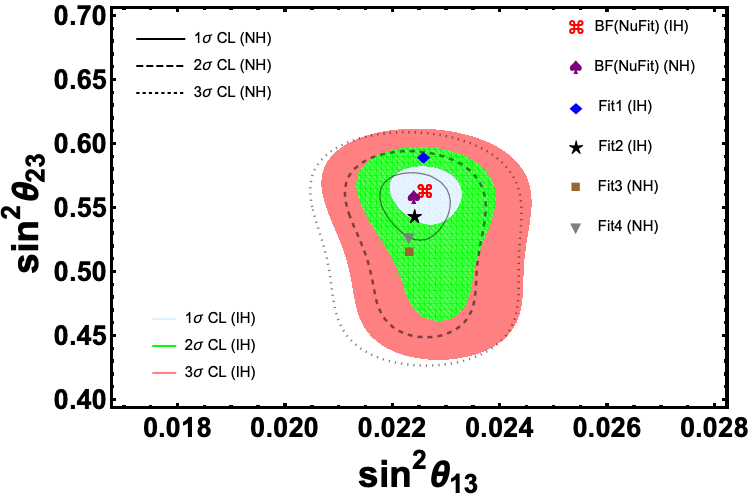
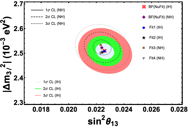
The input parameters shown in Table 7 provide excellent fits to the oscillation data, as can be seen in Table 7. For each of the benchmark points the phase in the PMNS matrix is large, showing that there is no restriction on its value. Fits 1 and 2 correspond to an inverted hierarchy, whereas Fits 3 and 4 represent a normal hierarchy. The benchmark points (Fit 1, Fit 2, Fit 3 and Fit 4) are also displayed in Fig. 2 as Fit1 (IH), Fit2 (IH), Fit3 (NH), and Fit4 (NH) as blue, black, brown, and gray markers respectively in various two-dimensional projections of the global-fit results Esteban:2018azc .
IV.3 Neutrinoless double beta Decay
In the standard framework with only light neutrinos contributing to , the amplitude for the rate is proportional to the element of the neutrino mass matrix, given by
| (87) |
Here , , and are the masses of the three light neutrinos, while , (for ), and (, ) are the two unknown Majorana phases.
We can apply Eq. (87) to our framework to determine its implications for . Since the determinant of vanishes owing to its skew-symmetric structure, the lightest neutrino is exactly massless. For a given mass ordering (normal or inverted), the masses of the heavier two neutrinos can then be determined from the observed mass splittings. The expression for the effective Majorana mass given in Eq. (87) then reduces to one of the following equations, depending on whether the hierarchy is normal or inverted:
| (88) | |||||
| (89) |
Note that only one Majorana phase (or one specific linear combination of phases) is relevant, due to the smallest mass eigenvalue being zero.
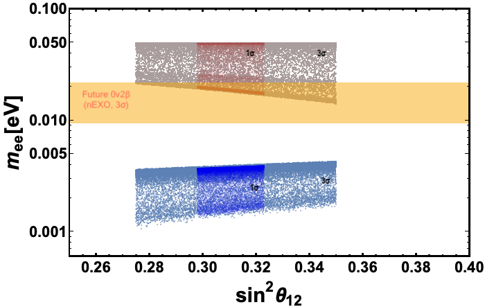
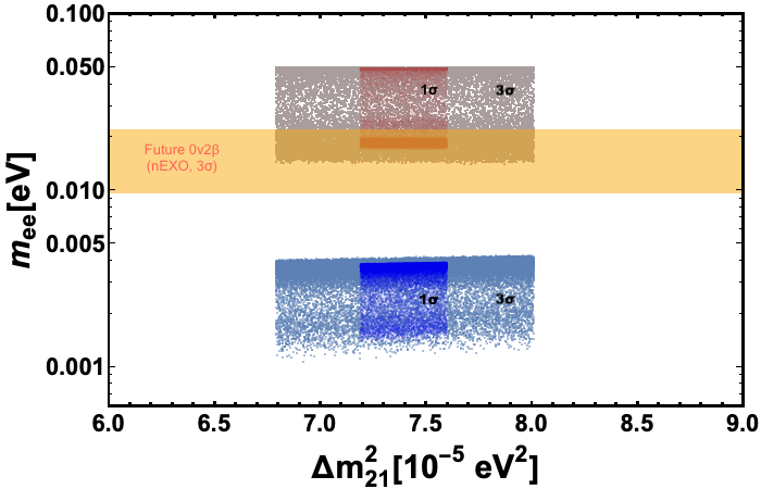
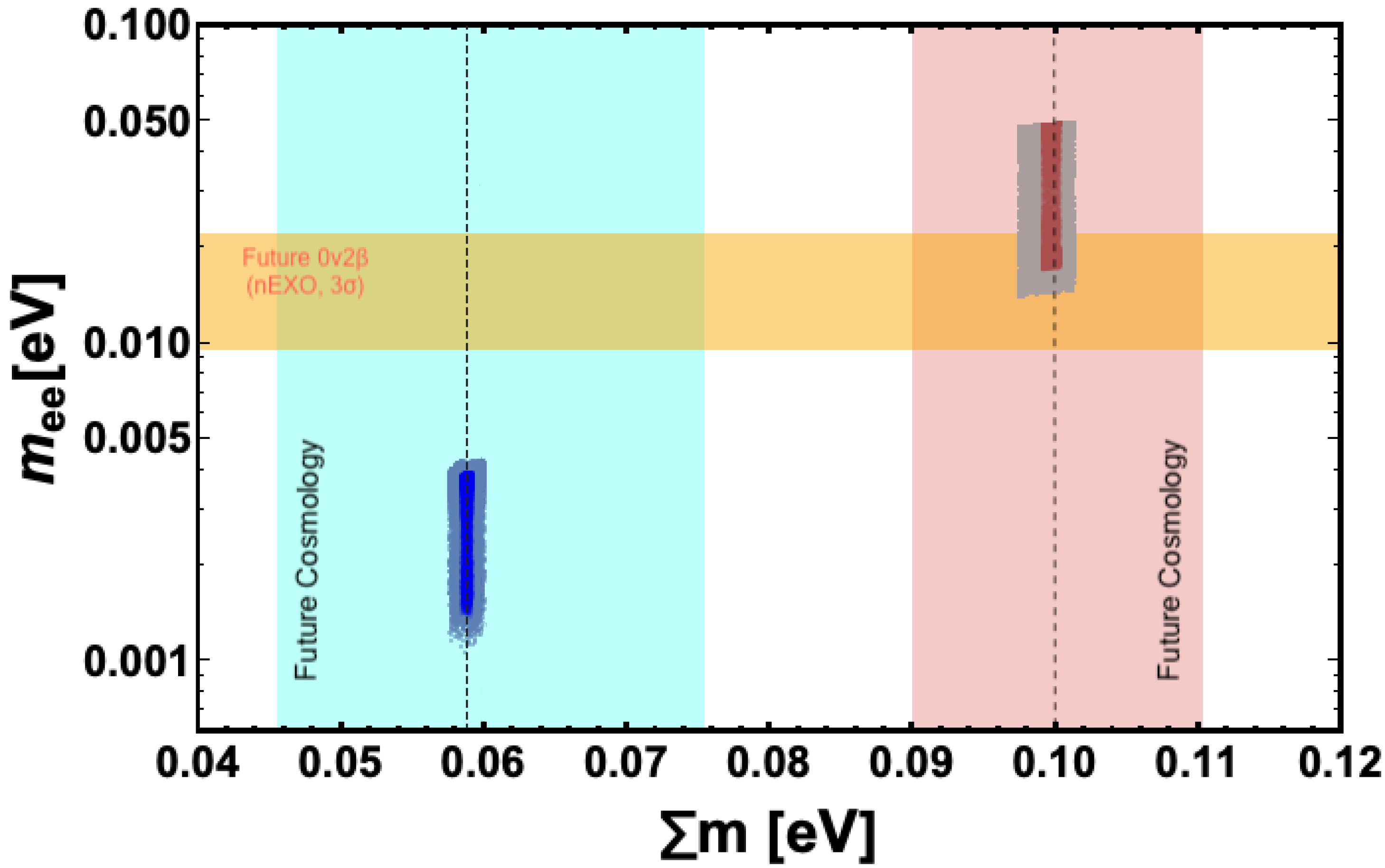
To illustrate the range of possibilities for in this class of models, in Fig. 3 we plot the effective Majorana mass as a function of , and the sum of light neutrino masses . We restrict to points that lie within and of the allowed oscillation parameter range. Each data point in Fig. 3 represents a valid fit that has been obtained by scanning over the input parameters shown in Eq. (86). For the purposes of this scan, we have taken all the elements of the matrix to be complex. Here the blue (red) points correspond to the case of normal (inverted) hierarchy. The Majorana phases, as well as the other observables in Eqs. (88) and (89), have been obtained as predictions of the points in the scan. First, the PMNS matrix is identified with the matrix diagonalizing , where is given in Eq. (86). Then, taking gives the diagonalized mass matrix with the appropriate Majorana phases.
We can use Eqs. (88) and (89) to obtain upper and lower limits on the rate of in this class of models. In the case of a normal hierarchy, the two terms in Eq. (88) add constructively for , while partial cancellation occurs for . The most effective cancellation (addition) happens when . This allows us to calculate the minimum and maximum values of the effective Majorana mass, which is parameterized as
| (90) |
Allowing the fit values from to vary over the range, the minimum effective Majorana mass is obtained as eV, whereas the maximum effective Majorana mass is . One can make similar arguments in the case of an inverted hierarchy, for which the most effective cancellation (enhancement) happens when in Eq. (89). This leads to
| (91) |
This allows us to determine the minimum and maximum values of the effective Majorana mass in the case of an inverted mass hierarchy as eV and eV respectively.
Future ton-scale experiments such as LEGEND Abgrall:2017syy and nEXO Albert:2017hjq should be able to probe the entire parameter space of this class of models if the hierarchy is inverted. For illustration, we show in Fig. 3 the future sensitivity from nEXO Albert:2017hjq at CL (horizontal orange band), where the band takes into account the nuclear matrix element uncertainties involved in translating a given lower bound on the half-life into an upper bound on the effective Majorana mass parameter.
Similarly, a future cosmological measurement of the sum of the light neutrino masses would allow another test of the model predictions. Shown in the bottom panel of Fig. 3 are the sensitivity from CMB-S4 Abazajian:2019eic (vertical band) for both the normal hierarchy (blue) and inverted hierarchy (red). It is clear from the figure that the model predictions lie well within the sensitivity of CMB-S4, and so these measurements offer an opportunity to test this scenario.
V Conclusion
In summary, we have presented a framework for neutrino masses in GUTs that predicts a specific texture for the form of the leading contribution to the Dirac mass term. In this scenario, neutrinos can be either Dirac or Majorana particles. A concrete prediction in the Dirac case is that the mass hierarchy is inverted. In the Majorana case, on the other hand, both normal and inverted hierarchies are allowed. In both the Dirac and Majorana cases, the model makes cosmologically testable predictions regarding the sum of neutrino masses. Furthermore, in the case of Majorana neutrinos, this framework predicts lower and upper bounds on the rate of for both the normal and the inverted hierarchies. In the case of an inverted hierarchy, this prediction can be tested in future ton-scale experiments.
Note Added: While this work was in progress we received Ref. Li:2019qxy , which considers Majorana neutrino masses in the context of an intermediate scale model embedded in an GUT. Although based on the inverse seesaw framework, the resulting pattern of neutrino masses shares some of the features of our Majorana construction, including the skew-symmetric form of the Dirac mass term and a massless neutrino.
Acknowledgments
The work of ZC and RNM is supported in part by the National Science Foundation under Grant No. PHY-1914731. The work of BD is supported in part by the U.S. Department of Energy under Grant No. DE-SC0017987 and in part by the MCSS funds. The work of AT is supported in part by the US Department of Energy Grant Number DE-SC0016013. ZC is also supported in part by the US-Israeli BSF grant 2018236. The work of BD and AT was also supported by the Neutrino Theory Network Program under Grant No. DE-AC02-07CH11359. BD acknowledges the High Energy Theory group at Oklahoma State University for warm hospitality, where part of this work was performed.
References
- (1) Particle Data Group, M. Tanabashi et al., “Review of Particle Physics,” Phys. Rev. D98 (2018) no. 3, 030001.
- (2) X. Qian and P. Vogel, “Neutrino Mass Hierarchy,” Prog. Part. Nucl. Phys. 83 (2015) 1–30, arXiv:1505.01891.
- (3) M. J. Dolinski, A. W. Poon, and W. Rodejohann, “Neutrinoless Double-Beta Decay: Status and Prospects,” Ann. Rev. Nucl. Part. Sci. 69 (2019) 219–251, arXiv:1902.04097.
- (4) J. C. Pati and A. Salam, “Lepton Number as the Fourth Color,” Phys. Rev. D 10 (1974) 275–289. [Erratum: Phys.Rev.D 11, 703–703 (1975)].
- (5) H. Georgi and S. Glashow, “Unity of All Elementary Particle Forces,” Phys. Rev. Lett. 32 (1974) 438–441.
- (6) P. Langacker, “Grand Unified Theories and Proton Decay,” Phys. Rept. 72 (1981) 185.
- (7) A. Buras, J. R. Ellis, M. Gaillard, and D. V. Nanopoulos, “Aspects of the Grand Unification of Strong, Weak and Electromagnetic Interactions,” Nucl. Phys. B 135 (1978) 66–92.
- (8) H. Georgi, “The State of the Art—Gauge Theories,” AIP Conf. Proc. 23 (1975) 575–582.
- (9) H. Fritzsch and P. Minkowski, “Unified Interactions of Leptons and Hadrons,” Annals Phys. 93 (1975) 193–266.
- (10) J. E. Kim, “Reason for SU(6) Grand Unification,” Phys. Lett. B 107 (1981) 69–72.
- (11) M. Fukugita, T. Yanagida, and M. Yoshimura, “N anti-N Oscillation without Left-Right Symmetry,” Phys. Lett. B 109 (1982) 369–372.
- (12) LSST, P. A. Abell et al., “LSST Science Book, Version 2.0,” arXiv:0912.0201.
- (13) L. Amendola et al., “Cosmology and fundamental physics with the Euclid satellite,” Living Rev. Rel. 21 (2018) no. 1, 2, arXiv:1606.00180.
- (14) DESI, A. Aghamousa et al., “The DESI Experiment Part I: Science,Targeting, and Survey Design,” arXiv:1611.00036.
- (15) Simons Observatory, P. Ade et al., “The Simons Observatory: Science goals and forecasts,” JCAP 02 (2019) 056, arXiv:1808.07445.
- (16) CMB-S4, K. Abazajian et al., “CMB-S4 Science Case, Reference Design, and Project Plan,” arXiv:1907.04473.
- (17) Project 8, A. Ashtari Esfahani et al., “Determining the neutrino mass with cyclotron radiation emission spectroscopy—Project 8,” J. Phys. G 44 (2017) no. 5, 054004, arXiv:1703.02037.
- (18) Hyper-Kamiokande, K. Abe et al., “Hyper-Kamiokande Design Report,” arXiv:1805.04163.
- (19) DUNE, B. Abi et al., “The DUNE Far Detector Interim Design Report Volume 1: Physics, Technology and Strategies,” arXiv:1807.10334.
- (20) F. Vissani, “Signal of neutrinoless double beta decay, neutrino spectrum and oscillation scenarios,” JHEP 06 (1999) 022, arXiv:hep-ph/9906525.
- (21) S. M. Bilenky, S. Pascoli, and S. Petcov, “Majorana neutrinos, neutrino mass spectrum, CP violation and neutrinoless double beta decay. 1. The Three neutrino mixing case,” Phys. Rev. D 64 (2001) 053010, arXiv:hep-ph/0102265.
- (22) R. N. Mohapatra et al., “Theory of neutrinos: A White paper,” Rept. Prog. Phys. 70 (2007) 1757–1867, arXiv:hep-ph/0510213.
- (23) A. Sen, “Sliding Singlet Mechanism in N=1 Supergravity GUT,” Phys. Lett. B 148 (1984) 65–68.
- (24) S. M. Barr, “The Sliding - singlet mechanism revived,” Phys. Rev. D 57 (1998) 190–194, arXiv:hep-ph/9705266.
- (25) Z. Berezhiani and G. Dvali, “Possible solution of the hierarchy problem in supersymmetrical grand unification theories,” Bull. Lebedev Phys. Inst. 5 (1989) 55–59.
- (26) R. Barbieri, G. Dvali, and M. Moretti, “Back to the doublet - triplet splitting problem,” Phys. Lett. B 312 (1993) 137–142.
- (27) G. Dvali, “Why is the Higgs doublet light?,” Phys. Lett. B 324 (1994) 59–65.
- (28) Z. Chacko and R. N. Mohapatra, “Doublet triplet splitting in supersymmetric SU(6) by missing VEV mechanism,” Phys. Lett. B 442 (1998) 199–202, arXiv:hep-ph/9809345.
- (29) R. Barbieri, G. Dvali, A. Strumia, Z. Berezhiani, and L. J. Hall, “Flavor in supersymmetric grand unification: A Democratic approach,” Nucl. Phys. B 432 (1994) 49–67, arXiv:hep-ph/9405428.
- (30) Z. Berezhiani, “SUSY SU(6) GIFT for doublet-triplet splitting and fermion masses,” Phys. Lett. B 355 (1995) 481–491, arXiv:hep-ph/9503366.
- (31) P. Minkowski, “ at a Rate of One Out of Muon Decays?,” Phys. Lett. B 67 (1977) 421–428.
- (32) R. N. Mohapatra and G. Senjanovic, “Neutrino Mass and Spontaneous Parity Nonconservation,” Phys. Rev. Lett. 44 (1980) 912.
- (33) T. Yanagida, “Horizontal gauge symmetry and masses of neutrinos,” Conf. Proc. C 7902131 (1979) 95–99.
- (34) M. Gell-Mann, P. Ramond, and R. Slansky, “Complex Spinors and Unified Theories,” Conf. Proc. C 790927 (1979) 315–321, arXiv:1306.4669.
- (35) I. Esteban, M. Gonzalez-Garcia, A. Hernandez-Cabezudo, M. Maltoni, and T. Schwetz, “Global analysis of three-flavour neutrino oscillations: synergies and tensions in the determination of , , and the mass ordering,” JHEP 01 (2019) 106, arXiv:1811.05487. http://www.nu-fit.org/.
- (36) T2K, K. Abe et al., “Constraint on the matter–antimatter symmetry-violating phase in neutrino oscillations,” Nature 580 (2020) no. 7803, 339–344, arXiv:1910.03887.
- (37) LEGEND, N. Abgrall et al., “The Large Enriched Germanium Experiment for Neutrinoless Double Beta Decay (LEGEND),” AIP Conf. Proc. 1894 (2017) no. 1, 020027, arXiv:1709.01980.
- (38) nEXO, J. Albert et al., “Sensitivity and Discovery Potential of nEXO to Neutrinoless Double Beta Decay,” Phys. Rev. C 97 (2018) no. 6, 065503, arXiv:1710.05075.
- (39) T. Li, J. Pei, F. Xu, and W. Zhang, “The Model from ,” arXiv:1911.09551.